Five lectures on DPG methods

Lecture Notes Jay Gopalakrishnan  
FIVE LECTURES ON DPG METHODS Spring 2013, Portland

These lectures present a relatively recent introduction into the class of discontinuos Galerkin (DG) methods, named Discontinuous Petrov-Galerkin (DPG) methods. DPG methods, in which DG spaces form a critical ingredient, can be thought of as least-square methods in nonstandard norms, or as Petrov-Galerkin methods with special test spaces, or as a nonstandard mixed method. We will pursue all these points of view in this lecture.

By way of preliminaries, let us recall two results from the Babuška-Brezzi theory. Throughout, $b(\cdot,\cdot):X\times Y\to\mathbb{C}$ is a continuous sesquilinear form where $X$ and $Y$ are (generally not equal) normed linear spaces over the complex field $\mathbb{C}$, $Y^{*}$ denotes the space of continuous conjugate-linear functionals on $Y$, and $\ell\in Y^{*}$.

Theorem 1.

Suppose $X$ is a Banach space and $Y$ is a reflexive Banach space. The following three statements are equivalent:

1. For any $\ell\in Y^{*}$, there is a unique $x\in X$ satisfying

   $$b(x,y)=\ell(y)\qquad\forall y\in Y.$$ (1)

2. $\{y\in Y:\;b(z,y)=0,\;\forall z\in X\}=\{0\}$ and there is a $C_{1}>0$ such that

   $$\inf_{0\neq z\in X}\sup_{0\neq y\in Y}\frac{|b(z,y)|}{\|z\|_{X}\|y\|_{Y}}\geq C_{1},$$ (2)

3. $\{z\in X:\;b(z,y)=0,\;\forall y\in Y\}=\{0\}$ and there is a $C_{1}>0$ such that

   $$\inf_{0\neq y\in Y}\sup_{0\neq z\in X}\frac{|b(z,y)|}{\|y\|_{Y}\|z\|_{X}}\geq C_{1}.$$ (3)

Theorem 2.

Suppose $X$ and $Y$ are Hilbert spaces, $X_{h}\subset X$ and $Y_{h}\subset Y$ are finite dimensional subspaces, $\dim(X_{h})=\dim(Y_{h})$, and suppose one of (a), (b) or (c) of Theorem 1 hold. If, in addition, there exists a $C_{3}>0$ such that

$$\inf_{0\neq z_{h}\in X_{h}}\sup_{0\neq y_{h}\in Y_{h}}\frac{|b(z_{h},y_{h})|}{\|y_{h}\|_{Y}}\geq C_{3},$$ (4)

then there is a unique $x_{h}\in X_{h}$ satisfying

$$b(x_{h},y_{h})=\ell(y_{h})\qquad\forall y_{h}\in Y_{h},$$ (5)

and

$$\|x-x_{h}\|_{X}\leq\frac{C_{2}}{C_{3}}\inf_{z_{h}\in X_{h}}\|x-z_{h}\|_{X},$$

where $C_{2}>0$ is any constant for which the inequality $|b(x,y)|\leq C_{2}\|x\|_{X}\|y\|_{Y}$ holds for all $x\in X$ and $y\in Y$.

We studied these well-known theorems in earlier lectures – see your earlier class notes for their full proofs and examples. Methods of the form (5) with $X_{h}\neq Y_{h}$ are called Petrov-Galerkin (PG) methods with trial space $X_{h}$ and test space $Y_{h}$. Note the standard difficulty: The inf-sup condition (2) does not in general imply the discrete inf-sup condition (4).

1. Optimal test spaces

Although (2)$\centernot\implies$ (4) in general, we now ask: Is it possible to find a test space $Y_{h}$ for which  (2)$\implies$ (4)? We now show that the answer is simple and affirmative. From now on, $X$ and $Y$ are Hilbert spaces, $(\cdot,\cdot)_{Y}$ denotes the inner product on $Y$, and $X_{h}$ is a finite-dimensional subspace of $X$ (where $h$ is some parameter related to the dimension).

Definition 3.

Given any trial space $X_{h}$, we define its optimal test space for the continuous sesquilinear form $b(\cdot,\cdot):X\times Y\to\mathbb{C}$ by

$$Y_{h}^{\mathrm{opt}}=T(X_{h})$$

where $T:X\to Y$ (the trial-to-test operator) is defined by

$$(Tz,y)_{Y}=b(z,y)\qquad\forall y\in Y,\;z\in X.$$ (6)

Equation (6) uniquely defines a $Tz$ for any given $z\in X$, by Riesz representation theorem. We call $Tz$ the “optimal” test function of $z$, because it solves an optimization problem, as we see next.

Proposition 4 (Optimizer).

For any $z\in X$, the maximum of

$$f_{z}(y)=\frac{|b(z,y)|}{\|y\|_{Y}}$$

over all nonzero $y\in Y$ is attained at $y=Tz$.

Proof.

By duality in Hilbert spaces,

$$\sup_{0\neq y\in Y}f_{z}(y) =\sup_{0\neq y\in Y}\frac{|(Tz,y)_{Y}|}{\|y\|_{Y}}=\|Tz\|_{Y},$$

and $f_{z}(Tz)=\|Tz\|_{Y}.$ ∎

Proposition 5 (Exact inf-sup condition $\implies$ Discrete inf-sup condition).

If (2) holds, then (4) holds with $C_{3}=C_{1}$ when we set $Y_{h}=Y_{h}^{\mathrm{opt}}$.

Proof.

For any $z_{h}\in X_{h}$, letting

$$s_{1}=\sup_{0\neq y\in Y}\frac{|b(z_{h},y)|}{\|y\|_{Y}},\qquad s_{2}=\sup_{0\neq y_{h}\in Y_{h}^{\mathrm{opt}}}\frac{|b(z_{h},y_{h})|}{\|y_{h}\|_{Y}}$$

it is obvious that $s_{1}\geq s_{2}$. To prove that $s_{1}\leq s_{2}$, since $s_{1}=\|Tz_{h}\|_{Y}$ by Proposition 4,

$$s_{1}=\|Tz_{h}\|_{Y}=\frac{|(Tz_{h},Tz_{h})_{Y}|}{\|Tz_{h}\|_{Y}}\leq\sup_{y_{h}\in Y_{h}^{\mathrm{opt}}}\frac{|(Tz_{h},y_{h})_{Y}|}{\|y_{h}\|_{Y}}=\sup_{y_{h}\in Y_{h}^{\mathrm{opt}}}\frac{|b(z_{h},y_{h})|}{\|y_{h}\|_{Y}}=s_{2},$$

so $s_{1}=s_{2}$. Hence the discrete inf-sup constant equals the exact inf-sup constant. ∎

Definition 6.

For any trial subspace $X_{h}\subset X$, the ideal PG method finds $x_{h}\in{X_{h}}$ solving

$$b({x_{h}},{y_{h}})=\ell({y_{h}}),\qquad\forall{y_{h}}\in Y_{h}^{\mathrm{opt}}.$$ (7)

Assumption 7.

Suppose $\{z\in X:\;b(z,y)=0,\;\forall y\in Y\}=\{0\}$ and suppose there exist $C_{1},C_{2}>0$ such that

$$C_{1}\|y\|_{Y}\leq\sup_{0\neq z\in X}\frac{|b(z,y)|}{\|z\|_{X}}\leq C_{2}\|y\|_{Y}\qquad\forall y\in Y.$$

The lower and upper inequalities are the exact inf-sup and continuity bounds, respectively.

Theorem 8 (Quasioptimality).

Assumption 7 $\implies$ the ideal PG method (7) is uniquely solvable for $x_{h}$ and

$$\|x-x_{h}\|_{X}\leq\frac{C_{2}}{C_{1}}\inf_{z_{h}\in X_{h}}\|x-z_{h}\|_{X}$$

where $x$ is the unique exact solution of (1).

Proof.

We want to apply Theorem 2. To this end, first observe that $T$ is injective: Indeed, if $Tz=0$, then by (6), we have $b(z,y)=0$ for all $y\in Y$, so Assumption 7 implies that $z=0$. Thus $\dim(X_{h})=\dim(Y_{h}^{\mathrm{opt}})$.

Furthermore, if the inf-sup condition of Assumption 7 holds, then it is an exercise (see Exercise 10 below) to show that the other inf-sup condition,

$$C_{1}\|z\|_{Y}\leq\sup_{0\neq y\in Y}\frac{|b(z,y)|}{\|y\|_{Y}}\qquad\forall z\in X,$$ (8)

holds with the same constant $C_{1}$. This, together with Proposition 5 shows that the discrete inf-sup condition (4) holds with the same constant. Hence Theorem 2 gives the result. ∎

Exercise 9.

Suppose $Z_{1},Z_{2}$ are Banach spaces and $A:Z_{1}\to Z_{2}$ is a linear continuous bijection. Then prove that the inverse of its dual $(A^{\prime})^{-1}$ exists, is continuous, and $(A^{\prime})^{-1}=(A^{-1})^{\prime}.$

Exercise 10.

Prove that, under the assumptions of Theorem 1, if Statement (c) of Theorem 1 holds for some $C_{1}$, then Statement (b) also holds with the same constant $C_{1}$. (Hint: Use Exercise 9 but do not forget that our spaces are over $\mathbb{C}$.)

Definition 11.

Let $R_{Y}:Y\to Y^{*}$ denote the Riesz map defined by $(R_{Y}y)(v)=(y,v)_{Y},$ for all $y$ and $v$ in $Y$. It is well known to be invertible and isometric:

$$\|R_{Y}y\|_{Y^{*}}=\|y\|_{Y}.$$ (9)

Let $B:X\to Y^{*}$ be the operator generated by the form $b(\cdot,\cdot)$, i.e., $Bx(y)=b(x,y)$ for all $x\in X$ and $y\in Y$. By the definition of $T$ in (6), it is obvious that

$$T=R_{Y}^{-1}\circ B.$$ (10)

Finally, for any $z\in X$, we define the energy norm of $z$ by $\vvvert{z}\vvvert_{X}\;\stackrel{{\scriptstyle\mathrm{def}}}{{=}}\;\|Tz\|_{Y}$. Clearly, by Proposition 4,

$$\vvvert{z}\vvvert_{X}=\|Tz\|_{Y}=\sup_{0\neq y\in Y}\frac{|b(z,y)|}{\|y\|_{Y}}.$$

Exercise 12.

Prove that if Assumption 7 holds, then $\vvvert{\cdot}\vvvert_{X}$ and $\|\cdot\|_{X}$ are equivalent norms:

$$C_{1}\|z\|_{X}\leq\vvvert{z}\vvvert_{X}\leq C_{2}\|z\|_{X}\qquad\forall z\in X.$$

Theorem 13 (Residual minimization).

Suppose Assumption 7 holds and $x$ solves (1). Then, the following are equivalent statements:

1. $x_{h}\in X_{h}$ is the unique solution of the ideal PG method (7).

2. $x_{h}$ is the best approximation to $x$ from $X_{h}$ in the following sense:

   $$\vvvert{x-x_{h}}\vvvert_{X}=\inf_{z_{h}\in X_{h}}\vvvert{x-z_{h}}\vvvert_{X}$$

3. $x_{h}$ minimizes residual in the following sense:

   $$x_{h}=\operatorname{arg}\min_{z_{h}\in X_{h}}\|\ell-Bz_{h}\|_{Y^{*}}.$$

Proof.

$(\ref{item:dpgls-1})\iff~{}(\ref{item:dpgls-2}):$

$$x_{h}\text{ solves~{}\eqref{eq:ipg}} \iff b(x-x_{h},y_{h})=0 \forall y_{h}\in Y_{h}^{\mathrm{opt}}$$

$$\iff b(x-x_{h},Tz_{h})=0 \forall z_{h}\in X_{h}$$

$$\iff(T(x-x_{h}),Tz_{h})_{Y}=0 \forall z_{h}\in X_{h},$$

and the result follows since $(T\cdot,T\cdot)_{Y}$ is the inner product generating the $\vvvert{\cdot}\vvvert_{X}$ norm.

$(\ref{item:dpgls-2})\iff~{}(\ref{item:dpgls-3}):$

$$\vvvert{x-x_{h}}\vvvert_{X}=\inf_{z_{h}\in X_{h}}\vvvert{x-z_{h}}\vvvert_{X} \iff\|T(x-x_{h})\|_{Y}=\inf_{z_{h}\in X_{h}}\|T(x-z_{h})\|_{Y}$$

$$\iff\|R_{Y}^{-1}B(x-x_{h})\|_{Y}=\inf_{z_{h}\in X_{h}}\|R_{Y}^{-1}B(x-z_{h})\|_{Y},$$ by (10),

$$\iff\|B(x-x_{h})\|_{Y^{*}}=\inf_{z_{h}\in X_{h}}\|B(x-z_{h})\|_{Y^{*}},$$ by (9),

$$\iff\|\ell-Bx_{h}\|_{Y^{*}}=\inf_{z_{h}\in X_{h}}\|\ell-Bz_{h}\|_{Y^{*}}$$

since $\ell=Bx$. This proves the result. ∎

Definition 14.

Let $x$ solve (1) and $x_{h}$ solve (7). We call $\varepsilon=R_{Y}^{-1}(\ell-Bx_{h})$ the error representation function. Clearly,

$$\|\varepsilon\|_{Y}=\|R_{Y}^{-1}B(x-x_{h})\|_{Y}=\|T(x-x_{h})\|_{Y}=\vvvert{x-x_{h}}\vvvert_{X},$$

i.e., the $Y$-norm of $\varepsilon$ measures the error in the energy norm. Note that $\varepsilon$ is the unique element of $Y$ satisfying

$$(\varepsilon,y)_{Y}=\ell(y)-b(x_{h},y),\qquad\forall y\in Y.$$

Theorem 15 (Mixed Galerkin formulation).

The following are equivalent statements:

1. $x_{h}\in X_{h}$ solves the ideal PG method (7).

2. $x_{h}$ and $\varepsilon$ solves the mixed formulation

   $$(\varepsilon,y)_{Y}+b(x_{h},y) =\ell(y) \forall y\in Y,$$ (11a)

   $$b(z_{h},\varepsilon) =0 \forall z_{h}\in X_{h}.$$ (11b)

Proof.

$(\ref{item:dpgmixed-1})\implies~{}(\ref{item:dpgmixed-2}):$ Since (11a) holds by the definition of the error representation function, we only need to prove (11b). To this end, $b(z_{h},\varepsilon)=(Tz_{h},\varepsilon)_{Y}=(Tz_{h},R_{Y}^{-1}(\ell-Bx_{h}))_{Y}=(Tz_{h},T(x-x_{h}))_{Y}$, which being the conjugate of $b(x-x_{h},Tz_{h})$, vanishes.

$(\ref{item:dpgmixed-2})\implies~{}(\ref{item:dpgmixed-1}):$ Since (11a) implies $b(x_{h},y_{h})=\ell(y_{h})-(\varepsilon,y_{h})_{Y}$ for all $y_{h}\in Y_{h}^{\mathrm{opt}}$, it suffices to prove that $(\varepsilon,y_{h})_{Y}=0$ for all $y_{h}\in Y_{h}^{\mathrm{opt}}$: But this is obvious from

$$(Tz_{h},\varepsilon)_{Y} =b(z_{h},\varepsilon)=0 \forall z_{h}\in X_{h},$$

which holds by virtue of (11b). ∎

To summarize the theory so far, we have shown that there are test spaces that can pair with any given trial space to generate an ideal Petrov-Galerkin method that is guaranteed to be stable. Moreover, the discrete inf-sup constant of the method is the same as the exact inf-sup constant. We then showed, in Theorem 13, that the resulting methods are least square methods that minimize the residual in a dual norm. Finally, we also showed that the method can be interpreted as a (standard Galerkin rather than a Petrov-Galerkin) mixed formulation on $Y\times X_{h}$, after introducing an error representation function.

Definition 16.

Suppose an open $\varOmega\subset\mathbb{R}^{N}$ is partitioned into disjoint open subsets $K$ (called elements), forming the collection ${\varOmega_{h}}$ (called mesh), such that the union of $\bar{K}$ for all $K\in{\varOmega_{h}}$ is $\bar{\varOmega}.$ Let $Y(K)$ denote a Hilbert space of some functions on $K$ with inner product $(\cdot,\cdot)_{Y(K)}$. An ideal DPG method is an ideal PG method with

$$Y=\prod_{K\in{\varOmega_{h}}}Y(K),$$ (12)

endowed with the inner product

$$(y,v)_{Y}=\sum_{K\in{\varOmega_{h}}}(y|_{K},v|_{K})_{Y(K)}\qquad\forall y,v\in K,$$

where $y|_{K}$ denotes the $Y(K)$-component of any $y$ in the product space $Y$. For example, the space $Y=H^{1}(\varOmega)$ is not of the form (12), while $Y=H^{1}({\varOmega_{h}})\;\stackrel{{\scriptstyle\mathrm{def}}}{{=}}\;\{v\in L^{2}(\varOmega):v|_{K}\in H^{1}(K)$ for all $K\in{\varOmega_{h}}\}$ is of the form (12).

Such DPG methods are interesting due to the resulting locality of $T$. Note that to compute a basis for the optimal test space, we must solve (6) to compute $Tz$ for each $z$ in a basis of $X_{h}$. That equation, namely $(Tz,y)_{Y}=b(z,y)$, decouples into independent equations on each element, if $Y$ has the form (12). Indeed, the component of $Tz$ on an element $K$, say $t_{K}=Tz|_{K}$ can be computed (independently of other elements) by solving $(t_{K},y_{K})_{Y(K)}=b(z,y_{K})$ for all $y_{K}\in Y(K).$ The adjective discontinuous in the name “DPG” should no longer be a surprise since test spaces $Y$ of the form (12) admit (discontinuous) functions with no continuity constraints across element interfaces.

2. Examples and Connections

Although we presented the theory over $\mathbb{C}$ for generality (e.g., to cover harmonic wave propagation), it continues to apply for real-valued bilinear and linear forms (in place of sesquilinear and conjugate-linear forms). All the examples in this section are over $\mathbb{R}$.

Example 17 (Standard FEM).

Set

$$(v,w)_{Y} =\int_{\varOmega}\mathop{\mathrm{grad}}v\cdot\mathop{\mathrm{grad}}w\;,\quad X=Y=H_{0}^{1}(\varOmega),\quad\|u\|_{X}^{2}=\|u\|_{Y}^{2}=(u,u)_{Y},$$

and consider the standard weak formulation of the Dirichlet problem: For any given $F\in H^{-1}(\varOmega)$, find $u\in H_{0}^{1}(\varOmega)$ solving

$$b(u,v)=F(v),\qquad\forall v\in H_{0}^{1}(\varOmega),$$

where $b(u,v)=(u,v)_{Y}$. Clearly, in this case, the trial-to-test operator $T$ is the identity map $I$ on $X$. Hence, if we set $X_{h}$ to the standard Lagrange finite element subspace of $H_{0}^{1}(\varOmega)$ based on a finite element mesh, we get $Y_{h}^{\mathrm{opt}}=X_{h}$. Thus the standard finite element method uses an optimal test space. Since the form is coercive, it obviously satisfies Assumption 7, so the previously discussed theorems apply for this method.

Example 18 ($L^{2}$-based least-squares method).

Suppose $X$ is a Hilbert space and $A:X\to L^{2}(\varOmega)$ is a continuous bijective linear operator. Then setting $Y=L^{2}(\varOmega)$, the problem of finding a $u\in X$ such that $Au=f$, for any given $f\in Y$, can be put into a variational formulation by setting

$$b(u,v)=(Au,v)_{Y},\qquad\ell(v)=(f,v)_{Y}.$$

Then it is obvious that $Tu=Au,$ so $Y_{h}^{\mathrm{opt}}=AX_{h}$. It is also easy to verify that Assumption 7 holds: By the bijectivity of $A$,

uniqueness: $$z\in X,b(z,y)=0\;\forall\;y\in L^{2}(\varOmega)\implies Az=0\implies z=0,$$

inf-sup: $$\sup_{0\neq z\in X}\frac{|(Az,y)_{Y}|}{\|z\|_{X}}\geq\frac{|(y,y)_{Y}|}{\|A^{-1}y\|_{X}}\geq C_{1}\|y\|_{Y},$$

with $C_{1}=\|A^{-1}\|^{-1}$. Hence, Theorems 8 and 13 hold for this method.

Finally, since $B=R_{L^{2}(\varOmega)}A$ and $\ell=R_{L^{2}(\varOmega)}f$, by the isometry of the Riesz map, the residual minimization property of Theorem 13(iii) implies that for any trial subspace $X_{h}\subset X$, we have

$$x_{h}=\operatorname{arg}\min_{z_{h}\in X_{h}}\|f-Az_{h}\|_{L^{2}(\varOmega)},$$

i.e., in this example, the ideal PG method coincides with the standard $L^{2}(\varOmega)$-based least-squares method.

Example 19 (1D o.d.e. without integration by parts).

Let $\varOmega=(0,1)$, $f\in L^{2}(\varOmega)$. Consider the boundary value problem (where primes denote differentiation) to find $u(x)$ solving

$$u^{\prime} =f \text{ on }(0,1),$$ (13a)

$$u(0) =0 \text{(boundary condition at $x=0$)}.$$ (13b)

A Petrov-Galerkin variational formulation is immediately obtained by multiplying (13a) with an $L^{2}$ test function $v$ and integrating. The resulting forms are

$$b(u,v)=\int_{0}^{1}u^{\prime}v,\quad\ell(v)=\int_{0}^{1}fv,$$

and the spaces are

$$X=\{u\in H^{1}(0,1):\;u(0)=0\},\quad Y=L^{2}(0,1).$$

This now fits into the framework of Example 18. (Indeed, the operator

$$Au=u^{\prime},\quad A:X\to Y\text{ is a bijection,}$$ (14)

because for any $f\in Y$, the function $u(x)=\int_{0}^{x}f(s)\;ds$ is in $X$ and satisfies $Au=f$.) Hence, as already discussed in Example 18, this method reduces to a standard $L^{2}$-based least-squares method.

Example 20 (1D o.d.e. with integration by parts).

We consider the same boundary value problem as above, namely (13), but now develop a different variational formulation for it. Multiply (13a) by a test function $v\in C^{1}(\bar{\varOmega})$ and integrate by parts to get

$$-\int_{0}^{1}uv^{\prime}+u(1)v(1)-u(0)v(0)=\int_{0}^{1}fv$$

Using (13b) and letting the unknown value $u(1)$ to be a separate variable $\hat{u}_{1}$, to be determined, we have derived the variational equation

$$-\int_{0}^{1}uv^{\prime}+\hat{u}_{1}v(1)=\int_{0}^{1}fv.$$

We let the pair $(u,\hat{u}_{1})$ to be a group variable $z$, and fix an appropriate functional setting. Set the forms by

$$b(z,v)\equiv b(\,(u,\hat{u}_{1}),v)=\hat{u}_{1}v(1)-\int_{0}^{1}uv^{\prime},\qquad\ell(v)=\int_{0}^{1}fv,$$

the spaces by

$$X=L^{2}(\varOmega)\times\mathbb{R},\quad Y=H^{1}(\varOmega),\quad\text{where }\varOmega=(0,1),$$

and the norms by

$$\|z\|_{X}^{2} \equiv\|(u,\hat{u}_{1})\|_{X}^{2}=\|u\|_{L^{2}(\varOmega)}^{2}+|\hat{u}_{1}|^{2}$$

$$\|v\|_{Y}^{2} =\|v^{\prime}\|_{L^{2}(\varOmega)}^{2}+|v(1)|^{2}.$$ (15)

By Sobolev inequality, $v(1)$ makes sense for $v\in Y$, so the above set $b(\cdot,\cdot)$ and $\|\cdot\|_{Y}$ are well-defined. In fact (by Exercise 21), the above set norm $\|v\|_{Y}$ is equivalent to the standard $H^{1}(\varOmega)$ norm.

Next, let us verify Assumption 7. First, suppose $(u,\hat{u}_{1})$ satisfies

$$b(\,(u,\hat{u}_{1}),v)=0\quad\forall v\in Y.$$ (16)

Then, choosing $v\in\mathcal{D}(\varOmega)$, the set of infinitely differentiable compactly supported functions in $\varOmega$, we find that the distributional derivative $u^{\prime}$ vanishes. Hence $u\in H^{1}(\varOmega)$. Going back to a general $v\in Y$, we may now integrate equation (16) by parts to obtain

$$-u(1)v(1)+u(0)v(0)+\hat{u}_{1}v(1)=0.$$ (17)

Choosing $v(x)=1-x$, we obtain $u(0)=0$. Thus, $u$ solves (13) with zero data, so $u\equiv 0$ by (14). From (17) we also have $u(1)=\hat{u}_{1}$, which together with $u\equiv 0$ implies

$$\hat{u}_{1}=0,\qquad u=0.$$ (18)

Thus the uniqueness part of Assumption 7, $\{z\in X:\;b(z,y)=0,\;\forall y\in Y\}=\{0\}$ holds.

For the remaining parts, we begin by noting that by Cauchy-Schwarz inequality,

$$\sup_{z\in X}\frac{|b(z,v)|^{2}}{\|z\|_{X}^{2}} =\sup_{(u,\hat{u}_{1})\in X}\frac{\displaystyle{\left|\hat{u}_{1}v(1)-\int_{0}^{1}uv^{\prime}\right|^{2}}}{\|u\|_{L^{2}(\varOmega)}^{2}+|\hat{u}_{1}|^{2}}\leq\sup_{(u,\hat{u}_{1})\in X}\frac{\displaystyle{\left(|\hat{u}_{1}|^{2}+\|u\|_{L^{2}(\varOmega)}^{2}\right)\|v\|_{Y}^{2}}}{\|u\|_{L^{2}(\varOmega)}^{2}+|\hat{u}_{1}|^{2}}=\|v\|_{Y}^{2}$$

while on the other hand, given any $v\in Y$, choosing $u=-v^{\prime}$ and $\hat{u}_{1}=v(1)$, we get

$$\sup_{z\in X}\frac{|b(z,v)|^{2}}{\|z\|_{X}^{2}} =\sup_{(u,\hat{u}_{1})\in X}\frac{\displaystyle{\left|\hat{u}_{1}v(1)-\int_{0}^{1}uv^{\prime}\right|^{2}}}{\|u\|_{L^{2}(\varOmega)}^{2}+|\hat{u}_{1}|^{2}}\geq\frac{\displaystyle{\left||v(1)|^{2}+\int_{0}^{1}|v^{\prime}|^{2}\right|^{2}}}{\|-v^{\prime}\|_{L^{2}(\varOmega)}^{2}+|v(1)|^{2}}=\|v\|_{Y}^{2}$$

Thus Assumption 7 holds with $C_{1}=C_{2}=1$.

We can now calculate the optimal test space (see Exercise 22 below) for any given trial space. Let $P_{p}(\varOmega)$ denote the space of polynomials of degree at most $p$ on $\varOmega$. We experiment with

$$X_{h}=P_{p}(\varOmega)\times\mathbb{R},$$

i.e., the discrete solution $x_{h}=(u_{h},\hat{u}_{1,h})$ has $u_{h}$ in $P_{p}(\varOmega)\subset L^{2}(\varOmega)$ and the point flux value approximation $\hat{u}_{1,h}$ in $\mathbb{R}$. The resulting method was implemented in FEniCS (code can be downloaded from here). Collecting the results obtained with an $f$ corresponding to an exact solution with a sharp layer,

$$u=\frac{e^{M(x-1)}-e^{-M}}{1-e^{-M}},$$

we obtain Figure 1.

The first graph in Figure 1 plots the exact solution $u$ and the computed $u_{h}$ for three values of $p$. We also implemented the method of Example 19 and plotted the corresponding solutions in the next graph in Figure 1. Comparing, we find that the ideal PG method of the current example performs better than that of Example 19. Finally, we also plotted the $L^{2}(\varOmega)$-projections of the exact solution on $P_{p}(\varOmega)$ in the last graph in Figure 1. Comparing the plots, the first and the third figures appear identical. Exercise 23 asks you to show that this is indeed the case.

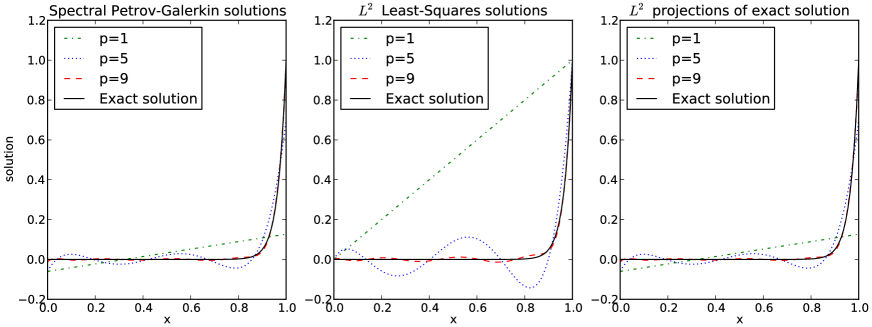
Figure 1. Solutions from one-element one-dimensional computations

Exercise 21.

Prove that the norm defined in (15) is equivalent to the standard Sobolev norm defined by $\|v\|^{2}_{H^{1}(\varOmega)}=\|v\|_{L^{2}(\varOmega)}^{2}+\|v^{\prime}\|_{L^{2}(\varOmega)}^{2}$. Hint: Use a Sobolev inequality and a Poincaré-type inequality.

Exercise 22.

Prove that in the setting of Example 20, an explicit formula for $T(u,\hat{u}_{1})$ can be given for any $(u,\hat{u}_{1})\in X$:

$$T(u,\hat{u}_{1})=\hat{u}_{1}+\int_{x}^{1}u(s)\,ds.$$ (19)

Next, use (41) to prove that if $X_{h}=P_{p}(\varOmega)\times\mathbb{R}$, then $Y_{h}^{\mathrm{opt}}=P_{p+1}(\varOmega)$.

Exercise 23.

Prove that the $u_{h}$ resulting from the ideal Petrov-Galerkin method of Example 20 equals the $L^{2}(0,1)$ projection of $u$ and that $\hat{u}_{1,h}=\hat{u}_{1}$. Hint: Apply Theorem 8.

Exercise 24.

Suppose $\varOmega=(0,1)$ is partitioned by the mesh $0=x_{0}<x_{1}<\cdots<x_{m}=1$. Consider the method of Example 20, modified to use the different trial subspace $X_{h}=\{u:u|_{(x_{i-1},x_{i})}\in P_{p}(x_{i-1},x_{i}),$ for $i=1,\ldots,m\}\times\mathbb{R}$. Show that $T$ does not, in general, map locally supported trial functions to locally supported test functions, by exhibiting a $(u,\hat{u}_{1})\in X_{h}$ such that $\mathop{\mathrm{missing}}{supp}(u)\subseteq[x_{i-1},x_{i}]$ for some $i$ but $\mathop{\mathrm{missing}}{supp}(T(u,\hat{u}_{1}))\not\subseteq[x_{i-1},x_{i}]$.

Example 25 (An ideal DPG method).

Continuing to consider (13), we now sketch how to extend the ideal PG scheme of Example 20 to an ideal DPG scheme. Following the setting of Definition 16, we assume $\varOmega=(0,1)$ is partitioned into ${\varOmega_{h}}$ consisting of $m$ intervals $(x_{i-1},x_{i})$ for all $i=1,\ldots,m$, with $x_{0}=0$ and $x_{m}=1$. Let $v^{\pm}(x)$ denote the limiting value of $v$ at $x$ from the right and left, respectively. Set

$$Y =H^{1}({\varOmega_{h}})=\{z\in L^{2}(\varOmega):z|_{K}\in H^{1}(K),\;\forall K\in{\varOmega_{h}}\}$$

$$\|y\|_{Y}^{2} =\sum_{i=1}^{m}\left(|y^{-}(x_{i})|^{2}+\int_{x_{i-1}}^{x_{i}}|y^{\prime}|^{2}\right)$$

$$X =L^{2}(\varOmega)\times\mathbb{R}^{m}$$

$$\|(u,{\hat{u}}_{1},{\hat{u}}_{2},\ldots,{\hat{u}}_{m})\|_{X}^{2} =\|u\|_{L^{2}(\varOmega)}^{2}+|\hat{u}_{1}|^{2}+|\hat{u}_{2}|^{2}+\cdots+|\hat{u}_{m}|^{2}$$

$$\ell(y) =(f,y)_{L^{2}(\varOmega)}$$

$$b(\,(u,{\hat{u}}_{1},{\hat{u}}_{2},\ldots,{\hat{u}}_{m}),\,y) =\sum_{i=1}^{m}\left({\hat{u}}_{i}y^{-}(x_{i})-{\hat{u}}_{i-1}y^{+}(x_{i-1})-\int_{x_{i-1}}^{x_{i}}uy^{\prime}\right),$$

with the understanding that ${\hat{u}}_{0}=0$. Note that if $m=1$, then this reduces to the method of Example 20. For general $m$, the action of the trial-to-test operator $T$ is local and can be computed element by element (see Exercise 26). The method for general $m$ can be analyzed as in Example 20 (see Exercise 27).

Exercise 26.

Prove that, in the setting of Example 25,

$$T(0,\cdots,0,\hat{u}_{i},0,\cdots,0)=\hat{u}_{i}\times\left\{\begin{aligned} &1&&\text{ if }x\in(x_{i-1},x_{i})\\ &x-x_{i+1}-1&&\text{ if }x\in(x_{i},x_{i+1})\\ &0&&\text{ elsewhere.}\end{aligned}\right.$$

Exercise 27.

Verify Assumption 7 for the formulation of Example 25.

The process by which we extended the formulation of Example 20 to that in Example 25 is an instance of “hybridization”. Variables like $\hat{u}_{i}$ in Example 25 are referred to by various names such as facet, or inter-element, or interface unknowns, and in the DG community, by names like numerical fluxes or numerical traces. To put the hybrid method in a more general PG context, we use the abstract setting stated next.

Assumption 28.

Suppose $X$ takes the form $X_{0}\times\hat{X}$ where $X_{0}$ and $\hat{X}$ are two Hilbert spaces and let the finite-dimensional subspace $X_{h}$ have the form $X_{h,0}\times\hat{X}_{h}$ with subspaces $X_{h,0}\subset X_{0}$ and $\hat{X}_{h}\subset\hat{X}$. Suppose there are continuous sesquilinear forms $\hat{b}(\cdot,\cdot):\hat{X}\times Y\to\mathbb{C}$ and $b_{0}(\cdot,\cdot):X_{0}\times Y\to\mathbb{C}$, in terms of which $b(\cdot,\cdot)$ is set by

$$b(\,(u,\hat{u}),y\,)=b_{0}(u,y)+\hat{b}(\hat{u},y),$$

for all $(u,\hat{u})\in X$ and $y\in Y$, and suppose

$$Y_{0}=\{y\in Y:\hat{b}(\hat{u}_{h},y)=0,\;\forall\hat{u}_{h}\in\hat{X}_{h}\}$$ (20)

is a closed subspace of $Y$. In addition to the already defined $T:X\to Y$, define $T_{0}:X_{0}\to Y_{0}$ by $(T_{0}u,y)_{Y}=b_{0}(u,y)$, for all $y\in Y_{0}.$

Under this setting, we consider two ideal PG methods:

$$\text{Find }(x_{h},\hat{x}_{h})\in X_{h}: \quad b(\,(x_{h},\hat{x}_{h}),y\,)=\ell(y) \forall y\in Y_{h}^{\mathrm{opt}}\equiv T(X_{h}).$$ (21a)

$$\text{Find }x_{h}\in X_{h,0}: \quad b_{0}(x_{h},y)=\ell(y) \forall y\in Y_{h,0}^{\mathrm{opt}}\equiv T_{0}(X_{h,0}).$$ (21b)

The interest in the “hybridized” form (21a) arises because, when moving from $Y_{0}$ to $Y$, one can often obtain test spaces of the form in Definition 16, which make $T$ local. This will become clearer in Example 30, discussed after the next theorem, and later in Example 55.

Theorem 29 (Hybrid method).

Suppose Assumption 28 holds. Then, the test spaces in (21) satisfy $Y_{h,0}^{\mathrm{opt}}\subset Y_{h}^{\mathrm{opt}}$. Hence,

$$(x_{h},\hat{x}_{h})\in X_{h}\text{ solves~{}\eqref{eq:15}}\implies x_{h}\text{ solves~{}\eqref{eq:16}.}$$

Proof.

Since $Y_{h}^{\mathrm{opt}}$ is a closed subspace of $Y$, we have the orthogonal decomposition

$$Y=Y_{h}^{\mathrm{opt}}+Y_{\perp}$$ (22)

where $Y_{\perp}$ is the $Y$-orthogonal complement of $Y_{h}^{\mathrm{opt}}$. Let $y_{0}\in Y_{h,0}^{\mathrm{opt}}$. Apply (22) to decompose $y_{0}=y_{h}+y_{\perp}$, with $y_{h}\in Y_{h}^{\mathrm{opt}}$ and $y_{\perp}\in Y_{\perp}$.

First, we claim that $y_{\perp}\in Y_{0}$. This is because

$$\hat{b}(\hat{u}_{h},y_{\perp})=(T(0,\hat{u}_{h}),y_{\perp})_{Y}=0\qquad\forall\hat{u}_{h}\in\hat{X}_{h}.$$

The last identity followed from the orthogonality of $y_{\perp}$ to $T(X_{h})$.

Next, we claim that $y_{\perp}=0$. It suffices to prove that $(y_{0},y_{\perp})_{Y}=0$ since $\|y_{\perp}\|_{Y}^{2}=(y_{0},y_{\perp})_{Y}$. Since $y_{0}\in Y_{h,0}^{\mathrm{opt}}$, there is a $u_{h}\in X_{h}$ such that $y_{0}=T_{0}u_{h}$. Then,

$$(y_{0},y_{\perp})_{Y} =(T_{0}u_{h},y_{\perp})_{Y}=b_{0}(u_{h},y_{\perp}) \text{as }y_{\perp}\in Y_{0}$$

$$=(T(u_{h},0),y_{\perp})_{Y}=0 \text{as }T(X_{h})\perp y_{\perp}.$$

Finally, since $y_{\perp}=0$, we have $y_{0}=y_{h}+0\in Y_{h}^{\mathrm{opt}}.$ Thus $Y_{h,0}^{\mathrm{opt}}\subset Y_{h}^{\mathrm{opt}}$. The second statement of the theorem is now obvious by choosing $y\in Y_{h,0}^{\mathrm{opt}}$ in (21a). ∎

Example 30.

Set $\varOmega=(0,1)$, $X_{0}=L^{2}(\varOmega)\times\mathbb{R},\hat{X}=\hat{X}_{h}=\mathbb{R}^{m-1},Y=H^{1}({\varOmega_{h}}),$

$$b_{0}(\,(u,\hat{u}_{m}),y) ={\hat{u}}_{m}y^{-}(1)-\sum_{i=1}^{m}\int_{x_{i-1}}^{x_{i}}uy^{\prime},$$

$$\hat{b}(\,(\hat{u}_{1},\ldots,\hat{u}_{m-1}),y) =\hat{u}_{1}y^{-}(x_{1})-\hat{u}_{m-1}y^{+}(x_{m-1})+\sum_{i=2}^{m-1}\left({\hat{u}}_{i}y^{-}(x_{i})-{\hat{u}}_{i-1}y^{+}(x_{i-1})\right),$$

Then, the method (21a) yields the method of Example 25. It is easy to see that $Y_{0}=H^{1}(\varOmega)$. Hence the method (21b) yields the method of Example 20. By Theorem 29, the (global basis of) optimal test functions of Example 20 can be expressed as a linear combination of the (local basis of) optimal test functions of Example 25.

3. Inexact test spaces

To compute the optimal test spaces, we need to apply $T$, which requires solving (6), typically an infinite-dimensional problem. Although we have seen some examples where the action of $T$ can be computed in closed form, for the vast majority of interesting boundary value problems, this is not feasible. Hence we are motivated to substitute the optimal test functions by inexact (approximations of) optimal test functions.

Let $Y^{r}$ denote a finite-dimensional subspace of $Y$ (with the index $r$ related to its dimension.) Let $T^{r}:X\to Y^{r}$ be defined by $(T^{r}w,y)_{Y}=b(w,y)$ for all $y\in Y^{r}$. In general, $T^{r}\neq T$.

Definition 31.

A DPG method for (1) uses a space $Y$ as in the ideal DPG method of Definition 16, finite-dimensional subspaces $X_{h}\subset X$ and $Y^{r}\subset Y$, and computes $x_{h}$ in $X_{h}$ satisfying

$$b({x_{h}},{y})=\ell({y}),\qquad\forall{y}\in Y_{h}^{r}\;\stackrel{{\scriptstyle\mathrm{def}}}{{=}}\;T^{r}(X_{h}).$$ (23)

The DPG method is sometimes also called the “practical” DPG method, because it uses the inexact, but practically computable, test space $Y_{h}^{r}$ (in contrast to the ideal DPG method, which uses the exact optimal test space $Y_{h}^{\mathrm{opt}}$).

Assumption 32.

There is a linear operator $\varPi:Y\to Y^{r}$ and a $C_{\varPi}>0$ such that for all ${w_{h}}\in{X_{h}}$ and all $v\in Y$,

$$b(w_{h},v-{\varPi}v)=0,\qquad\text{and}\qquad\|{\varPi}v\|_{Y}\leq C_{{\varPi}}\|v\|_{Y}.$$

Theorem 33.

Suppose Assumptions 7 and 32 hold. Then the DPG method (23) is uniquely solvable for $x_{h}$ and

$$\|x-x_{h}\|_{X}\leq\frac{C_{2}C_{\varPi}}{C_{1}}\inf_{z_{h}\in X_{h}}\|x-z_{h}\|_{X}$$

where $x$ is the unique exact solution of (1).

Proof.

First, note that by Assumption 32, $T^{r}:X_{h}\to Y^{r}$ is injective: $T^{r}w_{h}=0$ for some $w_{h}\in X_{h}\implies b(w_{h},y^{r})=0$ for all $y^{r}\in Y^{r}\implies b(w_{h},\varPi y)=0$ for all $y\in Y\implies b(w_{h},y)=0$ for all $y\in Y$, which by Assumption 7 implies that $w_{h}=0$. Thus,

$$\dim(Y_{h}^{r})=\dim(X_{h}).$$

Next, for any $z_{h}\in X_{h}$, let

$$s_{0}=\sup_{0\neq y\in Y}\frac{|b(z_{h},y)|}{\|y\|_{Y}},\qquad s_{1}=\sup_{0\neq y\in Y^{r}}\frac{|b(z_{h},y^{r})|}{\|y^{r}\|_{Y}},\qquad s_{2}=\sup_{0\neq y\in Y_{h}^{r}}\frac{|b(z_{h},y_{h}^{r})|}{\|y_{h}^{r}\|_{Y}}.$$

The result will follow from Theorem 2 once we prove the discrete inf-sup condition

$$C_{1}C_{\varPi}^{-1}\|z_{h}\|_{X}\leq s_{2}.$$ (24)

We proceed to bound $\|z_{h}\|_{X}$ using $s_{0}$, then $s_{1}$, and finally $s_{2}$. Assumption 7 implies (by Exercise 10) that the inf-sup condition

$$C_{1}\|z_{h}\|_{X}\leq s_{0}$$

holds. Hence Assumption 32 implies

$$C_{1}\|z_{h}\|_{X} \leq\sup_{0\neq y\in Y}\frac{|b(z_{h},y)|}{\|y\|_{Y}}=\sup_{0\neq y\in Y}\frac{|b(z_{h},\varPi y)|}{\|y\|_{Y}} \forall z_{h}\in X_{h}$$

$$\leq\sup_{0\neq y\in Y}\frac{|b(z_{h},\varPi y)|}{C_{\varPi}^{-1}\|\varPi y\|_{Y}}\leq\sup_{0\neq y\in Y^{r}}\frac{|b(z_{h},y^{r})|}{C_{\varPi}^{-1}\|y^{r}\|_{Y}} \forall z_{h}\in X_{h},$$

i.e., we have proven the tighter inf-sup condition $C_{1}C_{\varPi}^{-1}\|z_{h}\|_{X}\leq s_{1}$. To finish the proof of (24), it only remains to tighten it further by proving that $s_{1}\leq s_{2}$. Analogous to Proposition 4, $s_{1}$ is attained at $T^{r}z_{h}$, so

$$s_{1}=\frac{(T^{r}z_{h},T^{r}z_{h})_{Y}}{\|T^{r}z_{h}\|_{Y}}\leq\sup_{0\neq y_{h}^{r}\in Y_{h}^{r}}\frac{(T^{r}z_{h},y_{h}^{r})_{Y}}{\|y_{h}^{r}\|_{Y}}=s_{2}.$$

This shows (24) and finishes the proof. ∎

Remark 34.

Although Theorem 33 has more hypotheses than Theorem 8,

$$\text{Theorem~{}\ref{thm:inex}}\implies\text{Theorem~{}\ref{thm:quasiopt}.}$$

Indeed, the ideal PG method is obtained by simply setting $Y^{r}=Y$, and in that case, the trivial operator $\varPi=I$ satisfies Assumption 32 with $C_{\varPi}=1$. (Note that Theorem 33 holds if we use any closed subspace $Y^{r}\subset Y$ in (23), not only finite-dimensional $Y^{r}$.)

Exercise 35 (Necessity & Sufficiency of Assumption 32).

Suppose Assumption 7 holds. If there is a $C_{0}>0$ such that for all $\ell\in(Y_{h}^{r})^{*}$ there exists a unique $x_{h}\in X_{h}$ satisfying (23) and moreover

$$\|x_{h}\|_{X}\leq C_{0}\|\ell\|_{(Y_{h}^{r})^{*}},$$

then the method (23) is called stable and $C_{0}$ is the stability constant of the method. Show that

$$\text{the method~{}\eqref{eq:pdpg} is stable}\iff\text{Assumption~{}\ref{asm:Pi} holds},$$

and relate the stability constant to the other constants.

Definition 36 (cf. Definition 11).

Let $\vvvert{x}\vvvert_{r}\;\stackrel{{\scriptstyle\mathrm{def}}}{{=}}\;\|T^{r}x\|_{Y}$. Let $R_{Y^{r}}:{Y^{r}}\to{(Y^{r})}^{*}$ be the Riesz map defined by $(R_{Y^{r}}y)(v)=(y,v)_{Y},$ for all $y$ and $v$ in ${Y^{r}}$. By the definition of $T^{r}$, it is easy to see that

$$T^{r}w=R_{Y^{r}}^{-1}Bw.$$ (25)

Theorem 37 (cf. Theorem 13).

Suppose Assumptions 7 and 32 hold and let $x$ solve (1). Then, the following are equivalent statements:

1. $x_{h}\in X_{h}$ is the unique solution of the DPG method (23).

2. $x_{h}$ is the best approximation to $x$ from $X_{h}$ in the following sense:

   $$\vvvert{x-x_{h}}\vvvert_{r}=\inf_{z_{h}\in X_{h}}\vvvert{x-z_{h}}\vvvert_{r}$$

3. $x_{h}$ minimizes residual in the following sense:

   $$x_{h}=\operatorname{arg}\min_{z_{h}\in X_{h}}\|\ell-Bz_{h}\|_{{(Y^{r})^{*}}}.$$

Proof.

Follow along the lines of proof of Theorem 13 but use (25) instead of (10). ∎

Definition 38 (cf. Definition 14).

Let $x$ solve (1). We call $\varepsilon^{r}=R_{Y^{r}}^{-1}(\ell-Bx_{h})$ the error estimator of an $x_{h}$ in $X_{h}$. It is easy to see that it is the unique element of $Y^{r}$ satisfying $(\varepsilon^{r},y)_{Y}=\ell(y)-b(x_{h},y),$ for all $y\in Y^{r}$.

Theorem 39 (cf. Theorem 15).

The following are equivalent statements:

1. $x_{h}\in X_{h}$ solves the DPG method (23).

2. $x_{h}\in X_{h}$ and $\varepsilon^{r}\in Y^{r}$ solve the mixed formulation

   $$(\varepsilon^{r},y)_{Y}+b(x_{h},y) =\ell(y) \forall y\in Y^{r},$$ (26a)

   $$b(z_{h},\varepsilon^{r}) =0 \forall z_{h}\in X_{h}.$$ (26b)

Proof.

Follow along the lines of the proof of Theorem 15. ∎

Exercise 40.

Prove that $\varepsilon^{r}$ is $Y$-orthogonal to $Y_{h}^{r}$.

Next, recall the setting of Assumption (28) with $b(\,(u,\hat{u}),y\,)=b_{0}(u,y)+\hat{b}(\hat{u},y).$ Analogous to (20), define

$$Y_{0}^{r}=\{y\in Y^{r}:\;\hat{b}(\hat{u}_{h},y)=0,\;\forall\hat{u}_{h}\in\hat{X}_{h}\}$$ (27)

and let $T_{0}^{r}:X_{0}\to Y_{0}^{r}$ be defined by $(T_{0}^{r}u,y)_{Y}=b_{0}(u,y)$ for all $y\in Y_{0}^{r}.$ Then consider the corresponding DPG methods:

$$\text{Find }(x_{h},\hat{x}_{h})\in X_{h}: \quad b(\,(x_{h},\hat{x}_{h}),y\,)=\ell(y) \forall y\in Y_{h}^{r}\equiv T^{r}(X_{h}).$$ (28a)

$$\text{Find }x_{h}\in X_{h,0}: \quad b_{0}(x_{h},y)=\ell(y) \forall y\in Y_{h,0}^{r}\equiv T_{0}^{r}(X_{h,0}).$$ (28b)

Theorem 41 (cf. Theorem 29).

Suppose Assumption 28 holds. Then, the test spaces satisfy $Y_{h,0}^{r}\subset Y_{h}^{r}$. Hence,

$$(x_{h},\hat{x}_{h})\in X_{h}\text{ solves~{}\eqref{eq:26}}\implies x_{h}\text{ solves~{}\eqref{eq:27}.}$$

Proof.

Proceed as in the proof of Theorem 29, after replacing $Y$ by $Y^{r}$, and $Y_{\perp}$ by the orthogonal complement of $Y_{h}^{r}$ in $Y^{r}$. ∎

Remark 42 (Some ways to implement DPG methods).

1. Choose a local basis for $X_{h}$, say $e_{j}$. Compute $v_{i}=T^{r}e_{i}$ (usually precomputed on a fixed reference element and mapped to physical elements). Then assemble the square matrix

   $$A_{ij}=b(e_{j},v_{i})$$ (29)

   by usual finite element techniques and solve.

2. Let $e_{j}$ be as in item (1) and additionally select a local basis for $Y^{r}$, say $y_{i}$. Assemble the rectangular (since $\dim X_{h}\leq\dim Y^{r}$ typically) matrix

   $$B_{ij}=b(e_{j},y_{i})$$

   and the (block-diagonal) Gram matrix $M_{lm}=(y_{l},y_{m})_{Y}$. (Again, their assembly can be done by precomputing element matrices on a fixed reference element and mapping to physical elements.) Then form the square matrix $A=B^{t}M^{-1}B.$ It is easy to see that this matrix equals (29), so we proceed as in item (1).

3. Let $e_{j}$ and $y_{i}$ be as in item (2). Assemble the matrices of (26) and solve. Since (26) is a standard Galerkin formulation, not a Petrov-Galerkin formulation, this technique requires no further explanation. We will opt for this method in the code in the next section.

Exercise 43.

Suppose the basis $e_{j}$ and the matrix $A$ are as in Remark 42(1). Prove that Assumptions 7 and 32 imply the spectral condition number of $A$ satisfies

$$\kappa(A)\leq\frac{\lambda_{1}}{\lambda_{0}}\frac{C_{2}^{2}C_{\varPi}^{2}}{C_{1}^{2}},$$

where $\lambda_{0},\lambda_{1}$ are positive numbers such that $\lambda_{0}\|\vec{\chi}\|_{2}^{2}\leq\|x\|_{X}^{2}\leq\lambda_{1}\|\vec{\chi}\|_{2}^{2}$ holds for all $x=\sum_{j}\chi_{j}e_{j}$ in $X_{h}$.

4. The Laplacian

Let $\varOmega$ be a bounded connected open subset of $\mathbb{R}^{N}$ for any $N\geq 2$ with Lipschitz boundary $\partial\varOmega$. We focus on the simple boundary value problem

$$-\Delta u =f \text{ on }\varOmega,$$ (30a)

$$u =0 \text{ on }\partial\varOmega.$$ (30b)

All functions are real-valued in this section. We assume we have a mesh ${\varOmega_{h}}$ as in Definition 16 and additionally assume that $\partial K$ is Lipschitz for all $K\in{\varOmega_{h}}$ (so that we may use trace theorems on each element), but the shape of the elements is unimportant for now.

To develop our PG formulation for (30), we set the test space by

$$Y=H^{1}({\varOmega_{h}})=\{v:\;v|_{K}\in H^{1}(K),\;\forall K\in{\varOmega_{h}}\}\equiv\prod_{K\in{\varOmega_{h}}}H^{1}(K),$$

$$(v,y)_{Y}=(v,y)_{\varOmega_{h}}+(\mathop{\mathrm{grad}}v,\mathop{\mathrm{grad}}y)_{\varOmega_{h}}.$$

Multiplying (30) by a $v\in Y$ and integrating by parts on any element $K\in{\varOmega_{h}}$, we obtain

$$\int_{K}\mathop{\mathrm{grad}}u\cdot\mathop{\mathrm{grad}}v-\int_{\partial K}(n\cdot\mathop{\mathrm{grad}}u)v=\int_{K}fv.$$ (31)

As usual, the integral over $\partial K$ must be interpreted as a duality pairing in $H^{1/2}(\partial K)$ if $u$ is not sufficiently regular. Summing up (31) over all $K\in{\varOmega_{h}}$ and letting $n\cdot\mathop{\mathrm{grad}}u$ be an independent unknown, denoted by $\hat{q}_{n}$, we derive the PG formulation. To state it precisely, we use these notations: Let $(r,s)_{\varOmega_{h}}=\sum_{K\in{\varOmega_{h}}}(r,s)_{K}$ where $(\cdot,\cdot)_{D}$, for any domain $D$, denotes the $L^{2}(D)$-inner product and $\langle{\ell,w}\rangle_{\partial{\varOmega_{h}}}=\sum_{K\in{\varOmega_{h}}}\langle{\ell,w}\rangle_{1/2,\partial K}$ where $\langle{\ell,\cdot}\rangle_{1/2,\partial K}$ denotes the action of a functional $\ell$ in $H^{-1/2}(\partial K)$. The PG weak formulation finds $(u,\hat{q}_{n})\in X$ satisfying

$$(\mathop{\mathrm{grad}}u,\mathop{\mathrm{grad}}v)_{\varOmega_{h}}-\langle{\hat{q}_{n},v}\rangle_{\partial{\varOmega_{h}}}=(f,v)_{\varOmega},\qquad\forall v\in Y,$$ (32)

where the trial space $X$ is defined as follows: First, define the element-by-element trace operator $\mathop{\mathrm{tr}_{n}}$ by

$$\mathop{\mathrm{tr}_{n}}:H(\mathop{\mathrm{missing}}{div},{\varOmega})\to\prod_{K\in{\varOmega_{h}}}H^{-1/2}(\partial K),\qquad\mathop{\mathrm{tr}_{n}}r|_{\partial K}=r\cdot n|_{\partial K}.$$

Here and throughout, $n$ generically denotes the unit outward normal of any domain under consideration. Now set

$$H^{-1/2}(\partial\varOmega_{h}) =\mathop{\mathrm{missing}}{ran}(\mathop{\mathrm{tr}_{n}}),$$ (33)

$$\|\hat{r}_{n}\|_{H^{-1/2}(\partial{\varOmega_{h}})} =\inf\bigg{\{}\|q\|_{H(\mathop{\mathrm{missing}}{div},{\varOmega})}:\;\forall q\in H(\mathop{\mathrm{missing}}{div},{\varOmega})\text{ such that }\mathop{\mathrm{tr}_{n}}(q)=\hat{r}_{n}\bigg{\}}.$$

The trial space is then given by

$$X =H_{0}^{1}(\varOmega)\times H^{-1/2}(\partial{\varOmega_{h}}),$$

$$\|(w,\hat{r}_{n})\|_{X}^{2} =\|\mathop{\mathrm{grad}}w\|_{L^{2}(\varOmega)}^{2}+\|\hat{r}_{n}\|_{H^{-1/2}(\partial{\varOmega_{h}})}^{2}.$$

In (33), the norm is a quotient norm (see Exercises 44–46). With this quotient norm, we will not need to explicitly use the subspace topology inherited from $\prod_{K}H^{-1/2}(\partial K)$.

Exercise 44.

Suppose $X_{1}$ and $X_{2}$ are linear spaces, $A:X_{1}\to X_{2}$ is a linear onto map, and let $\pi:X_{1}\to X_{1}/\ker A$ be the quotient map.

1. Prove that there is a unique linear one-to-one and onto map $\hat{A}:X_{1}/\ker A\to X_{2}$ such that $A=\hat{A}\circ\pi$.

2. If in addition, $X_{1}$ is a normed linear space and $\ker A$ is closed, then using the quotient norm $\|\pi(u)\|_{X_{1}/\ker A}=\inf_{w\in\ker A}\|u+w\|_{X_{1}}$, prove that

   $$\|y\|_{X_{2}}=\|\hat{A}^{-1}y\|_{X_{1}/\ker A}$$ (34)

   makes $X_{2}$ into a normed linear space and $\hat{A}$ establishes an isometric isomorphism between $X_{1}/\ker A$ and $X_{2}$.

Exercise 45.

For all $r\in H(\mathop{\mathrm{missing}}{div},{\varOmega})$, define $\mathop{\mathrm{tr}_{n}}r\in H^{-1/2}(\partial{\varOmega_{h}})$ by $\mathop{\mathrm{tr}_{n}}r|_{\partial K}=r\cdot n|_{\partial K}$. What is $\ker(\mathop{\mathrm{tr}_{n}})$? Verify that $\ker(\mathop{\mathrm{tr}_{n}})$ is a closed subspace of $H(\mathop{\mathrm{missing}}{div},{\varOmega})$. Apply Exercise 44 with $X_{1}=H(\mathop{\mathrm{missing}}{div},{\varOmega})$, $X_{2}=H^{-1/2}(\partial{\varOmega_{h}})$, and $A=\mathop{\mathrm{tr}_{n}}$, to conclude that the norm in (33) is the same as (34), and that $H^{-1/2}(\partial{\varOmega_{h}})$ is complete under that norm.

Exercise 46.

Prove that there is a continuous linear map $E:H^{-1/2}(\partial{\varOmega_{h}})\to H(\mathop{\mathrm{missing}}{div},{\varOmega})$ such that $\|\hat{r}_{n}\|_{H^{-1/2}(\partial{\varOmega_{h}})}=\|E\hat{r}_{n}\|_{H(\mathop{\mathrm{missing}}{div},{\varOmega})}$ and $\mathop{\mathrm{tr}_{n}}E\hat{r}_{n}=\hat{r}_{n}$. (Hint: Consider $\hat{A}^{-1}$ from Exercise 44 and find a minimizer over a coset.)

We now set

$$b(\,(w,\hat{r}_{n}),\,v)=(\mathop{\mathrm{grad}}w,\mathop{\mathrm{grad}}v)_{\varOmega_{h}}-\langle{\hat{r}_{n},v}\rangle_{\partial{\varOmega_{h}}},\qquad\ell(v)=(f,v)_{\varOmega}$$

and proceed to analyze the formulation (32). Let $H(\mathop{\mathrm{missing}}{div},{{\varOmega_{h}}})=\{v\in L^{2}(\varOmega)^{N}:v|_{K}\in H(\mathop{\mathrm{missing}}{div},{K})$ for all $K\in{\varOmega_{h}}\}$. Define

$$\big{|}[\tau\cdot n]\big{|}_{\partial{\varOmega_{h}}} \;\stackrel{{\scriptstyle\mathrm{def}}}{{=}}\;\sup_{0\neq\phi\in H_{0}^{1}(\varOmega)}\frac{|\langle{\tau\cdot n,\phi}\rangle_{\partial{\varOmega_{h}}}|}{\;\|\phi\|_{H^{1}(\varOmega)}}, \forall\tau\in H(\mathop{\mathrm{missing}}{div},{{\varOmega_{h}}}),$$ (35)

$$\big{|}[vn]\big{|}_{\partial{\varOmega_{h}}} \;\stackrel{{\scriptstyle\mathrm{def}}}{{=}}\;\sup_{0\neq r\,\in H(\mathop{\mathrm{missing}}{div},{\varOmega})}\frac{|\langle{r\cdot n,v}\rangle_{\partial{\varOmega_{h}}}|}{\;\|r\|_{H(\mathop{\mathrm{missing}}{div},{\varOmega})}}, \forall v\in H^{1}({\varOmega_{h}}).$$ (36)

Exercise 47.

Prove that any $v\in H^{1}({\varOmega_{h}})$ has $\big{|}[vn]\big{|}_{\partial{\varOmega_{h}}}=0$ if and only if $v\in H_{0}^{1}(\varOmega)$.

Exercise 48.

Prove that $\displaystyle{\big{|}[vn]\big{|}_{\partial{\varOmega_{h}}}=\sup_{0\neq\hat{r}_{n}\in H^{-1/2}(\partial{\varOmega_{h}})}\frac{\!\!|\langle{\hat{r}_{n},v}\rangle_{\partial{\varOmega_{h}}}|}{\quad\|\hat{r}_{n}\|_{H^{-1/2}(\partial{\varOmega_{h}})}}.}$

Next, define an orthogonal projection $P:L^{2}(\varOmega)^{N}\to\mathop{\mathrm{grad}}H_{0}^{1}(\varOmega)$, by

$$(Pq,\mathop{\mathrm{grad}}\phi)_{\varOmega}=(q,\mathop{\mathrm{grad}}\phi)_{\varOmega}\qquad\forall\phi\in H_{0}^{1}(\varOmega).$$ (37)

Exercise 49.

Prove that $\mathop{\mathrm{grad}}H_{0}^{1}(\varOmega)$ is a closed subspace of $L^{2}(\varOmega)^{N}$ (under the current assumptions on $\varOmega$).

Lemma 50 (A Poincaré-type inequality).

There is a positive constant $C$ independent of ${\varOmega_{h}}$ such that for all $v$ in $H^{1}({\varOmega_{h}})$,

$$C\|v\|_{\varOmega_{h}}\leq\|P\mathop{\mathrm{grad}}v\|_{\varOmega_{h}}+\big{|}[vn]\big{|}_{\partial{\varOmega_{h}}}.$$

Proof.

Let $\phi$ in $H_{0}^{1}(\varOmega)$ solve the Dirichlet problem $-\Delta\phi=v$. Then,

$$\|v\|_{{L^{2}(\varOmega)}}^{2} =(-\Delta\phi,v)_{\varOmega}=(\mathop{\mathrm{grad}}\phi,\mathop{\mathrm{grad}}v)_{\varOmega_{h}}-\langle{\frac{\partial\phi}{\partial n},v}\rangle_{\partial{\varOmega_{h}}}$$

$$=(\mathop{\mathrm{grad}}\phi,P\mathop{\mathrm{grad}}v)_{\varOmega_{h}}-\langle{\frac{\partial\phi}{\partial n},v}\rangle_{\partial{\varOmega_{h}}}$$

$$\leq\|P\mathop{\mathrm{grad}}v\|_{\varOmega_{h}}\|\mathop{\mathrm{grad}}\phi\|_{\varOmega_{h}}+\bigg{(}\frac{\langle{\mathop{\mathrm{grad}}\phi\cdot n,v}\rangle_{\partial{\varOmega_{h}}}}{\quad\|\mathop{\mathrm{grad}}\phi\|_{H(\mathop{\mathrm{missing}}{div},{\varOmega})}}\bigg{)}\|\mathop{\mathrm{grad}}\phi\|_{H(\mathop{\mathrm{missing}}{div},{\varOmega})}$$

$$\leq\left(\|P\mathop{\mathrm{grad}}v\|_{\varOmega_{h}}+\sup_{q\in H(\mathop{\mathrm{missing}}{div},{\varOmega})}\!\!\frac{\langle{v,q\cdot n}\rangle_{\partial{\varOmega_{h}}}}{\quad\|q\|_{H(\mathop{\mathrm{missing}}{div},{\varOmega})}}\right)\|\mathop{\mathrm{grad}}\phi\|_{H(\mathop{\mathrm{missing}}{div},{\varOmega})}.$$

Since $\varOmega$ is bounded and connected, the standard Poincaré inequality holds, so $\|\mathop{\mathrm{grad}}\phi\|^{2}_{{L^{2}(\varOmega)}}\leq C\|v\|^{2}_{L^{2}(\varOmega)}$. Moreover, $\|\mathop{\mathrm{missing}}{div}(\mathop{\mathrm{grad}}\phi)\|_{L^{2}(\varOmega)}=\|v\|_{L^{2}(\varOmega)}$, so the result follows. ∎

Lemma 51 (Piecewise harmonic functions).

There is a $C>0$ independent of ${\varOmega_{h}}$ such that for all $v$ in $H^{1}({\varOmega_{h}})$ satisfying $\Delta(v|_{K})=0$ for all $K\in{\varOmega_{h}}$, we have

$$C\|\mathop{\mathrm{grad}}v\|_{\varOmega_{h}}\leq\big{|}[\mathop{\mathrm{grad}}v\cdot n]\big{|}_{\partial{\varOmega_{h}}}+\big{|}[vn]\big{|}_{\partial{\varOmega_{h}}}.$$

Proof.

Let $\tau=\mathop{\mathrm{grad}}v$. We construct the Helmholtz-Hodge decomposition of $\tau$, namely $\tau=\mathop{\mathrm{grad}}\psi+z$ with $\psi$ in $H_{0}^{1}(\varOmega)$ and $z$ in $H(\mathop{\mathrm{missing}}{div},{\varOmega})$, as follows: First define $\psi$ by

$$(\mathop{\mathrm{grad}}\psi,\mathop{\mathrm{grad}}\varphi)_{\varOmega}=(\tau,\mathop{\mathrm{grad}}\varphi)_{\varOmega_{h}},\qquad\forall\varphi\in H_{0}^{1}(\varOmega).$$ (38)

Then, set $z=\tau-\mathop{\mathrm{grad}}\psi$.

By (38), $(\tau-\mathop{\mathrm{grad}}\psi,\mathop{\mathrm{grad}}\varphi)_{\varOmega}=0$, so $\mathop{\mathrm{missing}}{div}z=0$. Hence the two components, $\mathop{\mathrm{grad}}\psi$ and $z,$ are $L^{2}(\varOmega)$-orthogonal and

$$\|z\|_{\varOmega}^{2}+\|\mathop{\mathrm{grad}}\psi\|^{2}_{\varOmega}=\|\tau\|_{\varOmega}^{2}.$$ (39)

Thus,

$$\|\tau\|_{\varOmega}^{2} =(\tau,\tau)=(\tau,\mathop{\mathrm{grad}}\psi+z)_{\varOmega_{h}}=(\tau,\mathop{\mathrm{grad}}\psi)_{\varOmega_{h}}+(\mathop{\mathrm{grad}}v,z)_{\varOmega_{h}}$$

$$=-(\mathop{\mathrm{missing}}{div}\tau,\psi)_{\varOmega_{h}}+\langle{\tau\cdot n,\psi}\rangle_{\partial{\varOmega_{h}}}+\langle{n\cdot z,v}\rangle_{\partial{\varOmega_{h}}},$$

Since $v$ is harmonic on each element, the first term vanishes. Hence

$$\|\tau\|_{\varOmega}^{2} =\frac{\langle{\tau\cdot n,\psi}\rangle_{\partial{\varOmega_{h}}}}{\|\psi\|_{H^{1}(\varOmega)}}\|\psi\|_{H^{1}(\varOmega)}+\frac{\langle{n\cdot z,v}\rangle_{\partial{\varOmega_{h}}}}{\|z\|_{H(\mathop{\mathrm{missing}}{div},{\varOmega})}}\|z\|_{L^{2}(\varOmega)}$$

$$\leq\bigg{(}\sup_{w\in H_{0}^{1}(\varOmega)}\frac{\langle{\tau\cdot n,w}\rangle_{\partial{\varOmega_{h}}}}{\|w\|_{H^{1}(\varOmega)}}\bigg{)}\|\psi\|_{H^{1}(\varOmega)}+\bigg{(}\sup_{q\in H(\mathop{\mathrm{missing}}{div},{\varOmega})}\frac{\!\langle{n\cdot q,v}\rangle_{\partial{\varOmega_{h}}}}{\quad\|q\|_{H(\mathop{\mathrm{missing}}{div},{\varOmega})}}\;\bigg{)}\|z\|_{L^{2}(\varOmega)}.$$

The result now follows from (39) and the standard Poincaré inequality applied to $\psi$. ∎

Lemma 52.

There is a positive constant $C$ independent of ${\varOmega_{h}}$ such that for all $v$ in $H^{1}({\varOmega_{h}})$,

$$\|\mathop{\mathrm{grad}}v\|_{\varOmega_{h}}\leq\|P\mathop{\mathrm{grad}}v\|_{\varOmega_{h}}+C\big{|}[vn]\big{|}_{\partial{\varOmega_{h}}}.$$

Proof.

Let $z\in H_{0}^{1}(\varOmega)$ be such that $P\mathop{\mathrm{grad}}v=\mathop{\mathrm{grad}}z$, let $\varepsilon=v-z$, and let $r|_{K}=-\mathop{\mathrm{grad}}(\varepsilon|_{K})$ on all $K\in{\varOmega_{h}}$. Then, (37) implies

$$(P\mathop{\mathrm{grad}}v-\mathop{\mathrm{grad}}v,\mathop{\mathrm{grad}}\phi)=(r,\mathop{\mathrm{grad}}\phi)_{K}=0\qquad\forall\phi\in H_{0}^{1}(\varOmega).$$ (40)

Choosing $\phi\in\mathcal{D}(K)$, we immediately find that $\mathop{\mathrm{missing}}{div}(r|_{K})=0$, i.e., $\varepsilon$ is harmonic on each $K\in{\varOmega_{h}}$. Applying Lemma 51, we thus obtain

$$C\|\mathop{\mathrm{grad}}\varepsilon\|_{\varOmega_{h}}\leq\big{|}[r\cdot n]\big{|}_{\partial{\varOmega_{h}}}+\big{|}[\varepsilon n]\big{|}_{\partial{\varOmega_{h}}}.$$ (41)

But $\big{|}[r\cdot n]\big{|}_{\partial{\varOmega_{h}}}=0$. This is because we may integrate by parts element by element to conclude from (40) that

$$0=(r,\mathop{\mathrm{grad}}\phi)_{\varOmega_{h}}=-(\mathop{\mathrm{missing}}{div}r,\phi)_{\varOmega_{h}}+\langle{r\cdot n,\phi}\rangle_{\partial{\varOmega_{h}}}=\langle{r\cdot n,\phi}\rangle_{\partial{\varOmega_{h}}},$$

for all $\phi\in H_{0}^{1}(\varOmega)$, so definition (35) implies $\big{|}[r\cdot n]\big{|}_{\partial{\varOmega_{h}}}=0$. Moreover, definition (36) shows that $\big{|}[\varepsilon n]\big{|}_{\partial{\varOmega_{h}}}=\big{|}[vn]\big{|}_{\partial{\varOmega_{h}}}$. Therefore, returning to (41), we conclude that

$$\|\mathop{\mathrm{grad}}v\|_{\varOmega_{h}}\leq\|P\mathop{\mathrm{grad}}v\|_{\varOmega_{h}}+\|\mathop{\mathrm{grad}}\varepsilon\|_{\varOmega_{h}}\leq\|P\mathop{\mathrm{grad}}v\|_{\varOmega_{h}}+C\big{|}[vn]\big{|}_{\partial{\varOmega_{h}}},$$

which proves the lemma. ∎

Theorem 53.

Assumption 7 holds for the formulation (32).

Proof.

The uniqueness part of Assumption 7, namely $\{(w,\hat{s}_{n})\in X:\;b(\,(w,\hat{s}_{n}),y)=0,\;\forall y\in Y\}=\{0\}$ can be proved by an argument analogous to what we have seen previously (see between (16) and (18)), so is left as an exercise.

To prove the continuity estimate, we use $|\langle{\hat{s}_{n},v}\rangle_{\partial{\varOmega_{h}}}|\leq\|\hat{s}_{h}\|_{H^{-1/2}(\partial{\varOmega_{h}})}\big{|}[vn]\big{|}_{\partial{\varOmega_{h}}}$, a consequence of Exercise 48, to get

$$|b(\,(w,\hat{s}_{n}),y)|\leq\|(w,\hat{s}_{n})\|_{X}\left(\|\mathop{\mathrm{grad}}v\|_{\varOmega_{h}}^{2}+\big{|}[vn]\big{|}_{\partial{\varOmega_{h}}}\right)^{1/2}$$

Now, since (36) implies

$$\big{|}[vn]\big{|}_{\partial{\varOmega_{h}}} =\sup_{r\,\in H(\mathop{\mathrm{missing}}{div},{\varOmega})}\frac{(r,\mathop{\mathrm{grad}}v)_{\varOmega_{h}}+(\mathop{\mathrm{missing}}{div}r,v)_{\varOmega_{h}}}{\;\|r\|_{H(\mathop{\mathrm{missing}}{div},{\varOmega})}}\leq\|v\|_{Y},$$

the continuity estimate is proved.

It only remains to prove the inf-sup condition. But

$$\sup_{\,(w,\hat{s}_{n})\in{{X}}}\frac{|b(\,(w,\hat{s}_{n}),v)|}{\|(w,\hat{s}_{n})\|_{{X}}} \geq\sup_{w\in H_{0}^{1}(\varOmega)}\frac{(\mathop{\mathrm{grad}}w,\mathop{\mathrm{grad}}v)_{\varOmega_{h}}}{\|\mathop{\mathrm{grad}}w\|_{L^{2}(\varOmega)}}=\|P\mathop{\mathrm{grad}}v\|_{L^{2}(\varOmega)},$$

$$\sup_{\,(w,\hat{s}_{n})\in{{X}}}\frac{|b(\,(w,\hat{s}_{n}),v)|}{\|(w,\hat{s}_{n})\|_{{X}}} \geq\sup_{\hat{s}_{n}\in H^{-1/2}(\partial{\varOmega_{h}})}\frac{|\langle{\hat{s}_{n},v}\rangle_{\partial{\varOmega_{h}}}|}{\|\hat{s}_{n}\|_{H^{-1/2}(\partial{\varOmega_{h}})}}=\big{|}[vn]\big{|}_{\partial{\varOmega_{h}}},$$

so the required inf-sup condition follows by adding and using Lemmas 52 and 50. ∎

To consider a particular instance of the DPG method, we now fix element shapes to be triangles. For any integer $p\geq 0$ let $P_{p}(K)$ denote the space of polynomials of degree at most $p$ restricted to $K$. For any triangle $K$, let $P_{p}(\partial K)$ denote the set of functions on $\partial K$ whose restrictions to each edge of $K$ is a polynomial of degree at most $p$. We now set

$$X_{h} =\{(w,\hat{s}_{n})\in X:\;w|_{K}\in P_{p+1}(K),\;\hat{s}_{n}|_{\partial K}\in P_{p}(\partial K)\;\;\forall K\in{\varOmega_{h}}\},$$ (42a)

$$Y^{r} =\{v\in Y:\;v|_{K}\in P_{r}(K),\;\;\forall K\in{\varOmega_{h}}\},$$ (42b)

compute the inexact test space $Y_{h}^{r}$, and consider the DPG method that finds $(u_{h},\hat{q}_{n,h})\in X_{h}$ solving

$$(\mathop{\mathrm{grad}}u_{h},\mathop{\mathrm{grad}}v)_{\varOmega_{h}}-\langle{\hat{q}_{n,h},v}\rangle_{\partial{\varOmega_{h}}}=(f,v)_{\varOmega},\qquad\forall v\in Y_{h}^{r}.$$ (43)

Theorem 54.

Suppose $N=2$, ${\varOmega_{h}}$ is a shape regular finite element mesh of triangles and $X_{h}$ and $Y^{r}$ are set as in (42). Then, whenever $r\geq p+N$, Assumption 32 holds. Consequently, by Theorem 33, the DPG method (43) is quasioptimal.

Proof.

Let $r=p+N$. It is easy to see that for every $v\in H^{1}(K)$, there is a unique $\varPi_{r}^{0}v\in P_{r}(K)$ satisfying

$$\varPi_{r}^{0}v =0 \text{at all 3 vertices of }K,$$

$$(\varPi_{r}^{0}v-v,q_{p-1})_{K} =0, \forall q_{p-1}\in P_{p-1}(K),$$

$$\langle\varPi_{r}^{0}v-v,\mu_{p}\rangle_{\partial K} =0, \forall\mu_{p}\in P_{p}(\partial K).$$

Setting $\varPi v=\varPi_{r}^{0}(v-\bar{v})+\bar{v}$, where $\bar{v}$ denotes the mean value of $v$ on $K$, it is an exercise to show that there is a $C$ independent of the size of the triangle $K$ (but dependent on the shape regularity of $K$) such that

$$(\varPi v-v,q_{p-1})_{K} =0, \forall q_{p-1}\in P_{p-1}(K),$$ (44a)

$$\langle\varPi v-v,\mu_{p}\rangle_{\partial K} =0, \forall\mu_{p}\in P_{p}(\partial K),$$ (44b)

$$\|\varPi v\|_{H^{1}(K)} \leq C\|v\|_{H^{1}(K)} \forall v\in H^{1}(K).$$ (44c)

Then,

$$b(\,(w_{h},\hat{s}_{n,h}),v-\varPi v) =(\mathop{\mathrm{grad}}w_{h},\mathop{\mathrm{grad}}(v-\varPi v))_{\varOmega_{h}}-\langle{\hat{s}_{n,h},v-\varPi v}\rangle_{\partial{\varOmega_{h}}}$$

$$=-(\Delta w_{h},v-\varPi v)_{\varOmega_{h}}-\langle{\hat{s}_{n,h}-n\cdot\mathop{\mathrm{grad}}w_{h},v-\varPi v}\rangle_{\partial{\varOmega_{h}}}=0,$$

by (44a) and (44b). ∎

Example 55.

To put this method into the framework of Assumption 28, set

$$X_{0}=H_{0}^{1}(\varOmega),\quad\hat{X}=H^{-1/2}(\partial{\varOmega_{h}}),$$

$$b_{0}(u,y)=(\mathop{\mathrm{grad}}u,\mathop{\mathrm{grad}}y)_{\varOmega_{h}},\quad\hat{b}(\hat{q}_{n},y)=-\langle{\hat{q}_{n},y}\rangle_{\partial{\varOmega_{h}}}.$$

Furthermore, the $X_{h}$ in (42a) can be split into $X_{h,0}\times\hat{X}_{h}$ with

$$X_{h,0} =\{w\in H_{0}^{1}(\varOmega):\;w|_{K}\in P_{p+1}(K),\;\;\forall K\in{\varOmega_{h}}\},$$

$$\hat{X}_{h} =\{\hat{s}_{n}\in H^{-1/2}(\partial{\varOmega_{h}}):\;\hat{s}_{n}|_{\partial K}\in P_{p}(\partial K)\;\;\forall K\in{\varOmega_{h}}\},$$

so that $Y_{0}$ in (20) becomes

$$Y_{0}=\{y\in H^{1}({\varOmega_{h}}):\langle{\hat{s}_{n,h},y}\rangle_{\partial{\varOmega_{h}}}=0,\;\forall\hat{s}_{n,h}\in\hat{X}_{h}\},$$

a weakly conforming subspace of $H^{1}(\varOmega)$. Its subspace, defined in (27) becomes $Y_{0}^{r}=\{y\in Y^{r}:\langle{\hat{s}_{n,h},y}\rangle_{\partial{\varOmega_{h}}}=0,\;\forall\hat{s}_{n,h}\in\hat{X}_{h}\}$. The non-hybrid form of the DPG method, namely (28b) uses this $Y_{0}^{r}$ and finds $u_{h}\in X_{h,0}$ satisfying

$$(\mathop{\mathrm{grad}}u_{h},\mathop{\mathrm{grad}}y_{0})_{\varOmega_{h}}=(f,y_{0})\qquad\forall y_{0}\in Y_{h,0}^{r}.$$ (45)

Recall that $y_{0}\in Y_{h,0}^{r}$ if and only if it is in $Y_{0}^{r}$ and solves

$$(\mathop{\mathrm{grad}}y_{0},\mathop{\mathrm{grad}}v)_{\varOmega_{h}}+(y_{0},v)_{\varOmega_{h}}=(\mathop{\mathrm{grad}}w,\mathop{\mathrm{grad}}v)_{\varOmega_{h}}\qquad\forall v\in Y^{r}$$ (46)

for some $w\in X_{h,0}$. By Theorem 41, the $u_{h}$ in (45) coincides with the first solution component of the hybrid DPG method (43). The difficulty with implementing (45) is that the computation of $Y_{h,0}^{r}$, requiring multiple solves of the global weakly conforming problem (46), is too expensive. In contrast the hybrid form (43) is easily implementable as the computation of $Y_{h}^{r}$ amounts to inverting a block diagonal matrix.

Before concluding, let us consider convergence rates. The error estimate of Theorem 33 (which holds by virtue of Theorems 53 and 54) gives

$$\|u-u_{h}\|_{H^{1}(\varOmega)}+\|\hat{q}_{n}-\hat{q}_{n,h}\|_{H^{-1/2}({\varOmega_{h}})}\leq C\inf_{(w_{h},\hat{s}_{n,h})\in X_{h}}\left(\|u-w_{h}\|_{H^{1}(\varOmega)}+\|\hat{q}_{n}-\hat{s}_{n,h}\|_{H^{-1/2}({\varOmega_{h}})}\right).$$

Henceforth $C>0$ denotes a generic constant independent of $h=\max_{K\in{\varOmega_{h}}}\mathop{\mathrm{missing}}{diam}(K)$ but dependent on the mesh’s shape regularity. To obtain convergence rates in terms of $h$, we must bound the infimum above. Suppose $u$ is smooth. By the Bramble-Hilbert lemma,

$$\inf_{w_{h}\in X_{h,0}}\|u-w_{h}\|_{H^{1}(\varOmega)}\leq Ch^{p+1}|u|_{H^{p+2}(\varOmega)}.$$ (47)

For the error in $\hat{q}_{n}$, let $q=\mathop{\mathrm{grad}}u$ and let $\mathop{\varPi_{\scriptscriptstyle{\mathrm{RT}}}}q$ denote the Raviart-Thomas projection of $q$ into $\{r\in H(\mathop{\mathrm{missing}}{div},{\varOmega}):r|_{K}\in P_{p}(K)+xP_{p}(K),\;\forall K\in{\varOmega_{h}}\}$. Then $\mathop{\varPi_{\scriptscriptstyle{\mathrm{RT}}}}q\cdot n\in\hat{X}_{h}$, so

$$\inf_{\hat{s}_{n,h}\in\hat{X}_{h}}\|\hat{q}_{n}-\hat{s}_{n,h}\|_{H^{-1/2}({\varOmega_{h}})}\leq\|(q-\mathop{\varPi_{\scriptscriptstyle{\mathrm{RT}}}}q)\cdot n\|_{H^{-1/2}({\varOmega_{h}})}\leq\|q-\mathop{\varPi_{\scriptscriptstyle{\mathrm{RT}}}}q\|_{H(\mathop{\mathrm{missing}}{div},{\varOmega})}$$

where we have used (33), by which, the $H^{-1/2}({\varOmega_{h}})$-norm of a function can be bounded by the $H(\mathop{\mathrm{missing}}{div},{\varOmega})$-norm of any of its extensions. Estimating $\|q-\mathop{\varPi_{\scriptscriptstyle{\mathrm{RT}}}}q\|_{H(\mathop{\mathrm{missing}}{div},{\varOmega})}$ as usual,

$$\inf_{\hat{s}_{n,h}\in\hat{X}_{h}}\|\hat{q}_{n}-\hat{s}_{n,h}\|_{H^{-1/2}({\varOmega_{h}})}\leq Ch^{p+1}\left(|q|_{H^{p+1}(\varOmega)}+|\mathop{\mathrm{missing}}{div}q|_{H^{p+1}(\varOmega)}\right).$$ (48)

From (47) and (48), we obtain $O(h^{p+1})$ convergence for $u_{h}$ and $\hat{q}_{n,h}$.

$h/\sqrt{2}$	$\|u-u_{h}\|_{H^{1}(\varOmega)}$	$\|\varepsilon^{r}\|_{H^{1}({\varOmega_{h}})}$
1/4	0.008277	0.008987
1/8	0.002111	0.002297
1/16	0.000531	0.000579
1/32	0.000133	0.000145
1/64	0.000033	0.000036

Let us now check if we see this convergence rate in practice. We use a FEniCS code (download code from here) which implements the mixed reformulation of the DPG method given in Theorem 39 (see also Remark 42). Solving a simple problem with a smooth solution (see the code for details) on the unit square, using $p=1$ and uniform meshes with various $h$, we collect the results in the table aside. Clearly, $\|u-u_{h}\|_{H^{1}(\varOmega)}$ appears to converge at $O(h^{2})$, in accordance with the theory. Also, the error estimator $\varepsilon^{r}$ (see Definition 38) appears to converge to zero at the same rate as the error.

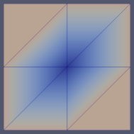
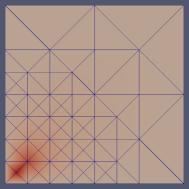
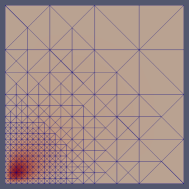
Figure 2. Initial, midway, and final iterates in an adaptive scheme using the DPG error estimator $\varepsilon^{r}$.

It is possible to prove that the error estimator $\varepsilon^{r}$ is an efficient and reliable indicator of the actual error, but to keep these lectures introductory, we omit the details. Instead, let us consider a FEniCS implementation of a typical adaptive algorithm using the element-wise norms of $\varepsilon^{r}$ as the error indicators (download the code from here). In the code, we compute the element error indicator $\|\varepsilon^{r}\|_{H^{1}(K)}$ on each $K\in{\varOmega_{h}}$, and sort the elements in decreasing order of the indicators. The elements falling in the top half are marked for refinement. In the next iteration of the adaptive algorithm, those elements (and possibly other adjacent elements) are refined by bisection, the DPG problem is solved on the new mesh, and the newly obtained $\varepsilon^{r}$ is used to mark elements as before. We use this process to approximate the solution of the Dirichlet problem (30) on the unit square with $f=e^{-100(x_{0}^{2}+x_{1}^{2})}.$ We expect the solution to have interesting variations only near the origin. As seen in Figure 2, the error estimator automatically identifies the right region for refinement even though we started with a very coarse mesh.

Appendix

Codes

The programs are in the python FEniCS environment. You will need to download and install FEniCS from fenicsproject.org for them to run. (I am not an expert in FEniCS and suggestions to improve the codes are very welcome.) Here are the available downloads on DPG methods:

• The FEniCS code for implementing the Petrov Galerkin method of Example 20 and generating Figure 1 can be downloaded from here. The code also implements a comparable least square method and the computation of $L^{2}$ projections.

• You can download download a FEniCS implementation of the DPG method for the Dirichlet problem.

• A code implementing an adaptive algorithm using the DPG error estimator is also available. This code is modeled after a FEniCS demo for standard finite elements.

Acknowledgments

These are (unpublished) notes from a few of my lectures in a Spring 2013 graduate class at PSU (MTH 610). The DPG research is in close collaboration with Leszek Demkowicz (see references below). I am grateful to my students for their feedback on the notes and to Kristian Ølgaard for clarifying FEniCS syntax. I am also grateful to NSF and AFOSR for supporting my research into DG and mixed methods and for encouraging the integration of such research into graduate education.

Bibliographic remarks

The presentation in Section 1, including the terminology of ‘optimal test spaces’, Theorem 8, etc. is based on [7]. The DPG methods were developed in a series of papers, beginning with [5, 7]. The name “DPG” was previously used by others [1], but without the concept of optimal test functions. The interpretation as a mixed formulation (Theorem 15) is motivated by [3]. Theorem 33 is from [9]. Operators such as $\varPi$, in the standard mixed Galerkin context, are sometimes known as Fortin operators. Theorems 29 and 41 have not appeared in this form previously. Lemmas 50 and 51 are from [6], but the method of Section 4 was developed later, independently in [8] and [2]. A more comprehensive bibliography is available in [4].

• [1] C. L. Bottasso, S. Micheletti, and R. Sacco. The discontinuous Petrov-Galerkin method for elliptic problems. Comput. Methods Appl. Mech. Engrg., 191(31):3391–3409, 2002.
• [2] D. Broersen and R. Stevenson, A Petrov-Galerkin discretization with optimal test space of a mild-weak formulation of convection-diffusion equations in mixed form, Preprint, 2013.
• [3] W. Dahmen, C. Huang, C. Schwab, and G. Welper. Adaptive Petrov-Galerkin methods for first order transport equations. SIAM J Numer. Anal., 50(5):2420–2445, 2012.
• [4] L. Demkowicz and J. Gopalakrishnan. An overview of the discontinuous Petrov Galerkin method. In X. Feng, O. Karakashian, and Y. Xing, editors, Recent Developments in Discontinuous Galerkin Finite Element Methods for Partial Differential Equations: 2012 John H Barret Memorial Lectures, volume 157 of The IMA Volumes in Mathematics and its Applications, pages 149–180. Institute for Mathematics and its Applications, Minneapolis, Springer, 2013.
• [5] L. Demkowicz and J. Gopalakrishnan. A class of discontinuous Petrov-Galerkin methods. Part I: The transport equation. Comput. Methods Appl. Mech. Engrg., 199:1558–1572, 2010.
• [6] L. Demkowicz and J. Gopalakrishnan. Analysis of the DPG method for the Poisson equation. SIAM J Numer. Anal., 49(5):1788–1809, 2011.
• [7] L. Demkowicz and J. Gopalakrishnan. A class of discontinuous Petrov-Galerkin methods. Part II: Optimal test functions. Numerical Methods for Partial Differential Equations, 27(1):70–105, 2011.
• [8] L. Demkowicz and J. Gopalakrishnan. A primal DPG method without a first-order reformulation. Computers and Mathematics with Applications, 66(6):1058–1064, 2013.
• [9] J. Gopalakrishnan and W. Qiu. An analysis of the practical DPG method. Math. Comp, in press, doi:10.1090/S0025-5718-2013-02721-4, electronically appeared, 2013.