HATS-3b: An inflated hot Jupiter transiting an F-type star

Abstract

We report the discovery by the HATSouth survey of HATS-3b, a transiting extrasolar planet orbiting a V=$12.4$ F dwarf star. HATS-3b has a period of $P=3.5479$ d, mass of $M_{p}=1.07$ $M_{\rm J}$, and radius of $R_{p}=1.38$ $R_{\rm J}$. Given the radius of the planet, the brightness of the host star, and the stellar rotational velocity ($v\sin{i}=9.0$ $\rm km\,s^{-1}$), this system will make an interesting target for future observations to measure the Rossiter-McLaughlin effect and determine its spin-orbit alignment. We detail the low/medium-resolution reconnaissance spectroscopy that we are now using to deal with large numbers of transiting planet candidates produced by the HATSouth survey. We show that this important step in discovering planets produces $\log{g}$ and $T_{\rm eff}$ parameters at a precision suitable for efficient candidate vetting, as well as efficiently identifying stellar mass eclipsing binaries with radial velocity semi-amplitudes as low as 1 $\rm km\,s^{-1}$.

1. Introduction

Transiting exoplanets provide us with the primary source of information about planets outside our own Solar System. These are the only planets for which we can routinely and accurately measure both mass and radius. In addition, they provide the possibility for further follow-up observations to measure other physical properties such as brightness temperature (e.g. Knutson et al., 2007), spin-orbit alignment (e.g. Queloz et al., 2000a), and atmospheric composition (e.g. Charbonneau et al., 2002).

There are 187 transiting exoplanets with published masses and radii, primarily discovered by the dedicated transit surveys of WASP (Pollacco et al., 2006), HATNet (Bakos et al., 2004), COROT (Auvergne et al., 2009), and Kepler (Borucki et al., 2010). A class of planets known as “hot Jupiters”, with short periods (P$<$10 d) and masses/radii similar to Jupiter, account for the majority of these discoveries. Hot Jupiters appear to be rare, occurring at a rate of around 0.4% around solar-type stars as determined by transit surveys (Bayliss & Sackett, 2011; Fressin et al., 2013). This rarity, coupled with the difficulty in detecting the $\sim$1% transit feature from a typical hot Jupiter, has meant that the task of building up a statistically significant set of hot Jupiters has progressed relatively slowly. However the task is important for two primary reasons. Firstly, individual systems can be studied in great detail to probe the nature of the exoplanet. Secondly, global trends for giant planets which require a statistically significant sample can be uncovered to better understand the formation and migration of planets.

The discovery of HATS-3b fits into both these categories. With a host star magnitude of V=$12.4$ it is a promising system for future spectroscopic and photometric follow-up studies, while it adds to the small set of known planets for which orbital and physical properties have been precisely measured.

The layout of the paper is as follows. In Section 2, we report the detection of the photometric signal and the follow-up spectroscopic and photometric observations of HATS-3. In Section 3, we describe the analysis of the data, beginning with the determination of the stellar parameters, continuing with a discussion of the methods used to rule out non-planetary, false positive scenarios which could mimic the photometric and spectroscopic observations, and finishing with a description of our global modelling of the photometry and radial velocities. The discovery of HATS-3b is discussed in Section 4, along with how it fits into the landscape of known hot Jupiters.

2. Observations

2.1. Photometric detection

Table 1 Summary of photometric observations

Facility	Date(s)	Number of Images	Cadence (s)	Filter
Discovery
HS-2 (Chile)	2009 Sep–2010 Sep	5660	284	Sloan $r$
HS-4 (Namibia)	2009 Sep–2010 Sep	8860	288	Sloan $r$
HS-6 (Australia)	2010 Aug–2010 Sep	198	288	Sloan $r$
Follow-Up
FTS/Spectral	2012 Jun 20	143	50	Sloan $i$
FTS/Spectral	2012 Jul 15	377	50	Sloan $i$
MPG/ESO2.2/GROND	2012 Aug 21	186	129	Sloan $g$
MPG/ESO2.2/GROND	2012 Aug 21	186	129	Sloan $r$
MPG/ESO2.2/GROND	2012 Aug 21	185	129	Sloan $i$
MPG/ESO2.2/GROND	2012 Aug 21	185	129	Sloan $z$

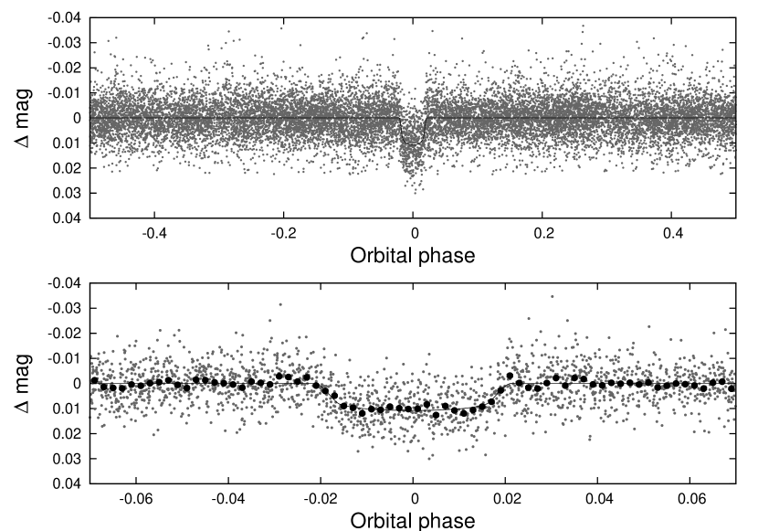
Figure 1.— The discovery light curve for HATS-3b. The top panel is the unbinned, relative, instrumental $r$-band light curve, phase-folded to the period $P=3.5478513$ days resulting from the global fit described in Section 3. The lower panel shows a zoom-in around the transit; dark filled circles are the light curve binned at 0.002 in phase. The solid line in both panels is the best-fit transit model (see Section 3). As a result of blending and our noise-filtering procedure, the transit detected in the HATSouth light curve for HATS-3 is 15% shallower than the true $r$-band transit.

The exoplanet HATS-3b was first identified as a transiting exoplanet candidate based on 14719 photometric observations of its host star HATS-3 (also known as 2MASS 20494978-2425436; $\alpha=20^{\mathrm{h}}49^{\mathrm{m}}49.80{\mathrm{s}}$, $\delta=-24{\arcdeg}25{\arcmin}43.7{\arcsec}$; J2000), from the HATSouth global network of automated telescopes (Bakos et al., 2013). The first three entries of Table 1 summarize these HATSouth discovery observations. For this particular candidate, observations were primarily performed by the HS2 and HS4 units (in Chile and Namibia respectively) over the period of a year from 2009 Sept to 2010 Sept. The HS6 unit (in Australia) only contributed a small number of images as it was under construction and commissioning during the period when the field containing HATS-3 was most intensively monitored by the HATSouth network.

Details relating to the observation, reduction, and analysis of the HATSouth photometric discovery data are fully described in Bakos et al. (2013). Here we provide a brief summary of the salient points.

The HATSouth observations consist of four-minute $r$-band exposures produced using 24 Takahashi E180 astrographs (18cm diameter primary mirrors) coupled to Apogee 4K$\times$4K U16M Alta CCDs. Photometry is performed using an aperture photometry pipeline and light curves are detrended using External Parameter Decorrelation (EPD; Bakos et al., 2010) and the Trend Filtering Algorithm (TFA) of Kovács et al. (2005). Light curves are searched for transit events using an implementation of the Box-fitting Least Squares algorithm (BLS; Kovács et al., 2002).

We detected a significant transit signal in the light curve of HATS-3 (see Figure 1). Based on this detection we initiated the multiphase follow-up procedure detailed below.

2.2. Reconnaissance Spectroscopy

The HATSouth global network of telescopes produces well over 100 candidates each year. To efficiently follow-up these candidates, we undertake a series of reconnaissance spectroscopic observations before attempting high-resolution spectroscopy. These reconnaissance observations consist of spectral typing candidates (Section 2.2.1) and medium-resolution radial velocities (Section 2.2.2). We summarize the reconnaissance spectroscopy observations taken for HATS-3 in Table 3.

2.2.1 Reconnaissance Spectral Typing

The aim of spectral classification during reconnaissance spectroscopy is to 1) efficiently identify and reject candidate host stars that are giants and therefore inconsistent (in our photometric regime) with the planet-star scenario, and 2) determine stellar parameters so that we can identify interesting transiting systems and prioritise the follow-up observations. For this purpose, a low-resolution spectrum is typically the first step in following up a HATSouth candidate.

A spectrum of HATS-3 was obtained using the Wide Field Spectrograph (WiFeS; Dopita et al., 2007) on the ANU 2.3 m telescope on 2012 April 10. WiFeS is a dual-arm image slicer integral field spectrograph. For spectral typing we use the blue arm with the B3000 grating, which delivers a resolution of R=$\lambda/\Delta\lambda$=3000 from 3500–6000 Å. Flux calibrations are performed according to Bessell (1999) using spectrophotometric standard stars from Hamuy et al. (1992) and Bessell (1999). A full description of the instrument configurations can be found in Penev et al. (2013).

The stellar properties $T_{\rm eff}$, $\log{g}$, $\rm[Fe/H]$, and interstellar extinction (E(B-V)) are derived via a grid search, minimising the $\chi^{2}$ between the observed spectrum and synthetic templates from the MARCS model atmospheres (Gustafsson et al., 2008). The search intervals are 250 K in $T_{\rm eff}$, 0.5 dex in $\log{g}$ and $\rm[Fe/H]$. A restricted $T_{\rm eff}$ search space is established using 2MASS J-K colours. Extinction is applied according to Cardelli et al. (1989), with E(B-V) values ranging from 0 to the maximum extinction from the Schlegel et al. (1998) maps. The $T_{\rm eff}$ – $\log{g}$ probability space for HATS-3 is plotted in Figure 2, along with observed spectrum and best fitting template.

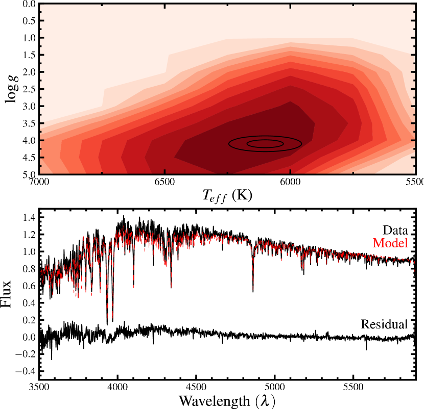
Figure 2.— Low resolution spectral classification of HATS-3 using WiFeS. Top: Contours marking the $T_{\rm eff}$ – $\log{g}$ probability space are shown. Typical 1 and 2$\sigma$ uncertainties for WiFeS-derived stellar parameters are shown. Bottom: The observed spectrum (black solid) is plotted against the best fitting template spectrum (red dashed), with residuals plotted beneath.

Since the differentiation of giants and dwarfs is of particular importance, we place more weight on the $\log{g}$ sensitive spectral features during the $\chi^{2}$ calculations. These regions include the MgH feature (e.g. Bell et al., 1985; Berdyugina & Savanov, 1994), the Mg b triplet (e.g. Ibata & Irwin, 1997) for cooler stars, and the Balmer jump for hotter stars (e.g. Bessell, 2007).

To estimate the uncertainties of the HATSouth reconnaissance spectral typing, we observed nine planet-hosting stars with published stellar parameters derived from high resolution spectroscopy (including the HATS-3 properties presented in this study). The range in $T_{\rm eff\star}$, $\log{g}$, $\rm[Fe/H]$ and V magnitude of these stars closely resemble the HATSouth candidates, so they serve as good bench markers. In addition, we also include six evolved stars with published stellar parameters from high resolution spectroscopy (de Medeiros et al., 2006). These stars have low $\log{g}$ values and demonstrate our ability to distinguish between giants and dwarfs. The results are presented in Table 2 and Figure 3. The root-mean-square deviation between the parameters derived from our WiFeS observations of the dwarf stars and their published parameters are $T_{\rm eff\star}$= 200 K, $\log{g}$= 0.35, and $\rm[Fe/H]$ = 0.44.

WiFeS low-resolution reconnaissance spectral classification revealed that HATS-3 is an F dwarf with $T_{\rm eff\star}=6200\pm 200\,K$, $\log{g_{\star}}=4.1\pm 0.4$, and $\rm[Fe/H]=-0.5\pm 0.4$. These values are consistent with the more precise values obtained from subsequent high resolution spectroscopy (subsection 2.3).

To gauge the level of contamination to HATSouth candidates by false positive scenarios involving giants, Figure 4 plots the histogram of the measured $\log{g}$ value for all candidates followed-up to date. We find that overall 12% of the 240 HATSouth candidates spectral typed to date are identified as giants ($\log g<3.5$) by our reconnaissance spectroscopy. For the expected galactic population, approximated using the Besançon model (Robin et al., 2003), within a field centred at $\alpha=300^{\circ}$, $\delta=−25^{\circ}$ and extending to 50 kpc distance, the giant occurrence rate is 24%. Our candidate identification system is not sensitive to planets orbiting giants (as these transit signatures are so diluted as to be undetectable), so any “transit” seen around a giant will generally either be red-noise mimicking a transit signal or scenarios in which a giant is belended with an eclipsing binary. The contribution of giants is greater for brighter candidates, as expected from the model population (see Figure 4). We find 35% of HATSouth candidates with magnitudes $9<V<12$ are giants, making reconnaissance spectral typing extremely valuable over this magnitude range.

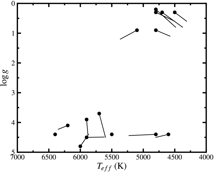
Figure 3.— Benchmarking the WiFeS spectral classifications. $T_{\rm eff\star}$and $\log{g}$ values derived from our WiFeS spectral classification are marked by solid points, the vectors point towards the corresponding published values as set out in Table 2.

Table 2 WiFeS Reconnaissance Spectral Typing Performance

Star	Reference	$T_{\rm eff}$	$\log{g}$	$\rm[Fe/H]$
WASP-4	Wilson et al. (2008)	5500(5500$\pm$150)	4.4 (4.45+0.016/-0.029)	0.0 (0.00$\pm$0.20)
WASP-5	Anderson et al. (2008)	5900 (5880$\pm$150)	3.9 (4.40+0.039/-0.048)	0.5 (0.09$\pm$0.09)
WASP-7	Hellier et al. (2009)	6400 (6400$\pm$100)	4.4 (4.36+0.01/-0.047)	-0.5 (0.00$\pm$0.1)
WASP-8	Queloz et al. (2010)	5700 (5600$\pm$80)	3.7 (4.50$\pm$0.1)	-0.5 (0.17$\pm$0.07)
WASP-29	Hellier et al. (2010)	4600 (4800$\pm$150)	4.4 (4.50$\pm$0.2)	0.0 (0.11$\pm$0.14)
WASP-46	Anderson et al. (2012)	5900 (5620$\pm$160)	4.5 (4.49$\pm$0.02)	0.0 (-0.37$\pm$0.13)
HATS-1	Penev et al. (2013)	6000 (5870$\pm$100)	4.8 (4.40$\pm$0.08)	-0.5 (-0.06$\pm$0.12)
HATS-2	Mohler-Fischer et al. (2013)	4800 (5227$\pm$95)	4.4 (4.44$\pm$0.12)	-0.5 (0.15$\pm$0.05)
HATS-3	This work.	6200 ($6351\pm 76$)	4.1 ($4.23\pm 0.0$)	-0.5 ($-0.157\pm 0.07$)
HD36702	de Medeiros et al. (2006)	4800 (4485$\pm$111)	0.2 (0.8$\pm$0.15)	-2.0 (-2.0$\pm$0.17)
HD29574	de Medeiros et al. (2006)	4500 (4310$\pm$111)	0.3 (0.6$\pm$0.15)	-2.0 (-1.9$\pm$0.17)
HD26297	de Medeiros et al. (2006)	4800 (4500$\pm$111)	0.3 (1.2$\pm$0.15)	-1.5 (-1.7$\pm$0.17)
HD20453	de Medeiros et al. (2006)	5100 (5365$\pm$111)	0.9 (1.2$\pm$0.15)	-1.5 (-2.0$\pm$0.17)
HD103036	de Medeiros et al. (2006)	4700 (4375$\pm$111)	0.3 (0.8$\pm$0.15)	-1.5 (-1.7$\pm$0.17)
HD122956	de Medeiros et al. (2006)	4800 (4575$\pm$111)	0.9 (1.1$\pm$0.15)	-2.0 (-1.8$\pm$0.17)

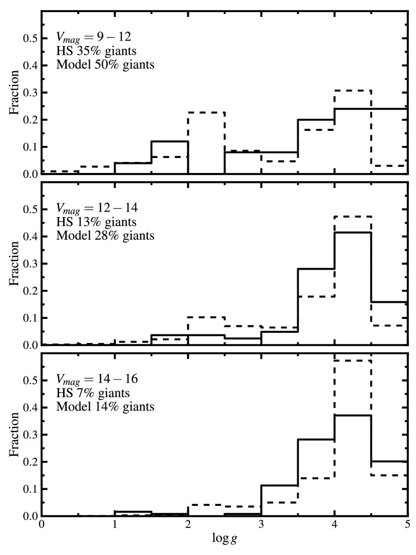
Figure 4.— Histograms showing the $\log{g}$ distribution for HATSouth candidates over different brightness bins. The candidate population is plotted by solid lines, the Besançon model population (Robin et al., 2003) is plotted in dashed lines for reference. The contribution by giants is noted in each brightness bin.

2.2.2 Reconnaissance WiFeS Radial Velocities

In addition to determining stellar parameters, we also use WiFeS on the ANU 2.3 m telescope to look for radial velocity variations above $\sim$2 $\rm km\,s^{-1}$. Such variations indicate the transiting body is typically a stellar-mass object rather than an exoplanet, and effectively rules out the candidate as a transiting exoplanet. The observations are timed to phase quadratures, where the expected velocity difference is greatest.

For radial velocity measurements, we use the red arm of the WiFeS spectrograph with the R7000 grating and RT480 dichroic. This results in $R\equiv\lambda/\Delta\lambda=7000$ over 5200–7000 Å. Wavelength solutions are provided by bracketing NeFeAr arc lamp exposures, with a further first order correction made using telluric Oxygen B band lines at 6882–6906 Å. Radial velocities are derived via cross correlation against RV standard stars (Nidever et al., 2002) exposures taken every night. Further details of the observing set-up and the data reduction pipeline can be found in (Penev et al., 2013).

Simultaneous radial velocities are also derived for any neighbours within the $12\times 38\arcsec$ WiFeS field of view. Significant velocity variations for any close-neighbours consistent with the photometric ephemeris are indicative of blended eclipsing binary scenarios, and are subsequently rejected.

To date 184 HATSouth candidates have been monitored using WiFeS multi-epoch radial velocities measurements with enough phase coverage to constrain any velocity variation at the 2 $\rm km\,s^{-1}$ level. We find 51 (27%) to be stellar mass binaries. Figure 5 presents the distribution of the radial velocity orbit semi-amplitude $(K)$ of these candidates. We find two peaks in the velocity amplitude, one at $\sim 10$ $\rm km\,s^{-1}$, representing the F-M stellar binary population, and another at $\sim 45$ $\rm km\,s^{-1}$, representing a larger mass ratio population that exhibits shallow grazing transits. In both scenarios, the resulting transit depth is similar to that of a planet-star system, and are identified as potential planetary systems from their discovery lightcurve. Figure 5 also presents the fraction of eclipsing stellar mass systems within our sample as a function of candidate $V$-band magnitude. We find a paucity of eclipsing binaries for the brighter candidates. The reason for this is that these lightcurves are of higher precision that allows better determination of the shape of the transit feature. Also, as was pointed out in Section 2.2.1, a higher fraction of the candidates are giants. There is an excess of eclipsing binaries for the faintest candidates, for which only deep transits can be identified from the lower precision discovery lightcurves. The large number of contaminating eclipsing binaries for the faintest candidates highlights the particular advantage of medium resolution observations in this regime. Although faint, these candidates are of interest to the HATSouth survey as they contain a high fraction of low mass stars that are not easily probed by other wide-field transit surveys.

We obtained one 500 s exposure on each of three consecutive nights from 2012 April 10 – 12 to measure the radial velocity for HATS-3 over its full phase. The radial velocities were clustered within 1 $\rm km\,s^{-1}$of each other on each night, indicating that the transiting body could not be of stellar mass.

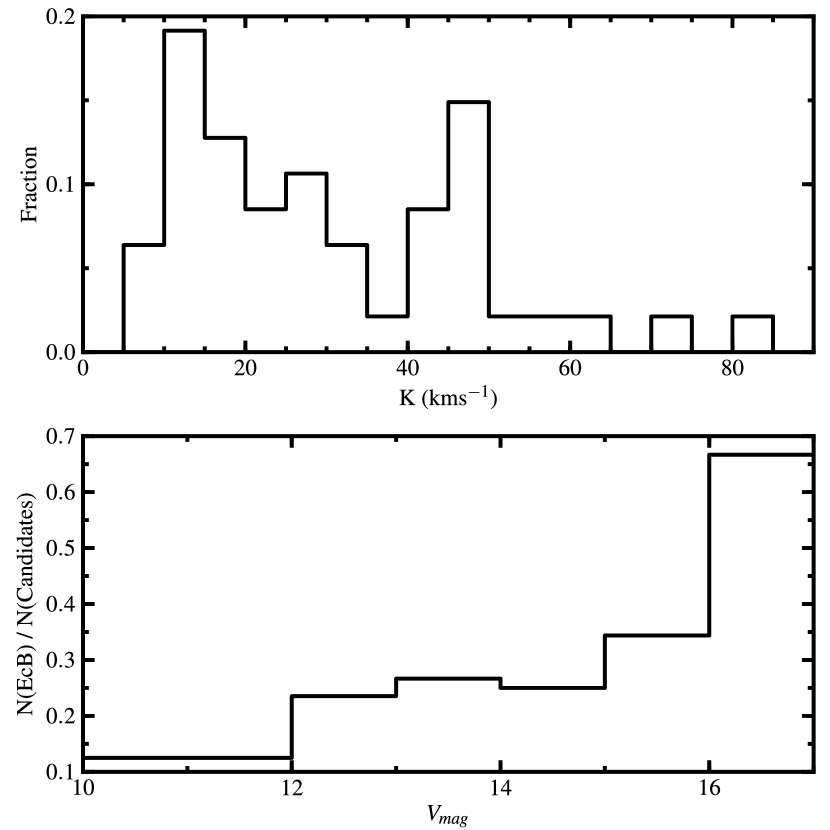
Figure 5.— Top: Distribution of radial velocity semi-amplitude $(K)$ for the stellar mass binaries identified from WiFeS medium resolution measurements. Bottom: Fractional contamination by eclipsing binaries in the HATSouth candidate population as a function of $V$ band magnitude.

2.3. High Resolution Spectroscopy

High-resolution spectroscopy is only carried out on candidates that pass the screening process involved with the reconnaissance spectroscopy set out in Section 2.2. This allows us to focus our time-intensive high-resolution spectroscopy on the targets that are most likely to host planets.

HATS-3 was monitored by three different echelle spectrographs capable of measuring high-precision radial velocities over the period 2012 April – June. Table 3 summarizes these high-resolution spectroscopic observations. Thirteen observations were taken with FEROS (Kaufer & Pasquini, 1998) on the MPG/ESO2.2 m telescope at La Silla Observatory, Chile. A further eight observations of HATS-3 were taken by both CORALIE (Queloz et al., 2000b) on the Swiss Leonard Euler 1 m telescope at La Silla Observatory, Chile, and UCLES (using the CYCLOPS fibre feed) on the 3.9 m AAT at Siding Spring Observatory, Australia. For a description of the observations and data reduction employed for these instruments, see Penev et al. (2013). The radial velocity measurements for these observations are set out in Table 4, and are plotted after phase-wrapping to the best-fit period (see Section 3) in Figure 6. Where possible we calculated the bisector spans of the cross-correlation functions, and they did not vary in phase with the radial velocity measurements.

Table 3 Summary of spectroscopic observations

Telescope/	Date	Number of	Exposure	Resolution	SNR	Wavelength
Instrument	Range	Observations	Times (s)			coverage (Å)
Reconnaissance
ANU 2.3 m/WiFeS	2012 Apr 10	1	300	3000	100	3500–6000
ANU 2.3 m/WiFeS	2012 Apr 10–12	3	500	7000	50	5200–7000
High Precision Radial Velocity
AAT 3.9 m/CYCLOPS	2012 May 5–11	8	1500	70000	20	4540–7340
Euler 1.2 m/Coralie	2012 Jun 2–7	8	1800	60000	20	3850–6900
MPG/ESO 2.2 m/FEROS	2012 Apr 1–Jun 8	13	2700	48000	20	3500–9200

Figure 6.— Top panel: Radial velocity measurements for HATS-3 from CORALIE (dark filled circles), FEROS (open triangles) and CYCLOPS (filled triangles) shown as a function of orbital phase, together with our best-fit circular (solid line) and eccentric (dotted line) models. Zero phase corresponds to the time of mid-transit. The center-of-mass velocity has been subtracted. Second panel: Velocity $O\!-\!C$ residuals from the best fit circular model. The error bars include a component from astrophysical/instrumental jitter allowed to differ for the three instruments.

Table 4 Relative radial velocity measurements of HATS-3.

BJD	RV	$\sigma_{\rm RV}$	Phase	Instrument
(2 454 000$+$)	($\rm m\,s^{-1}$)	($\rm m\,s^{-1}$)
$2019.89700$	$124$	$53$	$0.647$	FEROS
$2032.87600$	$36$	$108$	$0.305$	FEROS
$2035.90600$	$-77$	$45$	$0.159$	FEROS
$2036.88374$	$115$	$28$	$0.435$	Coralie
$2037.92527$	$155$	$33$	$0.729$	Coralie
$2040.85700$	$108$	$89$	$0.555$	FEROS
$2053.19936$	$-116$	$45$	$0.034$	AAT
$2053.32636$	$-180$	$94$	$0.070$	AAT
$2055.25949$	$4$	$27$	$0.614$	AAT
$2056.20988$	$161$	$29$	$0.882$	AAT
$2057.17510$	$-159$	$34$	$0.154$	AAT
$2057.32183$	$-20$	$29$	$0.196$	AAT
$2058.24637$	$-32$	$25$	$0.456$	AAT
$2059.25685$	$210$	$34$	$0.741$	AAT
$2076.83800$	$173$	$65$	$0.697$	FEROS
$2077.74700$	$84$	$99$	$0.953$	FEROS
$2078.76300$	$-163$	$64$	$0.239$	FEROS
$2079.79400$	$54$	$58$	$0.530$	FEROS
$2080.75400$	$149$	$61$	$0.800$	FEROS
$2080.83500$	$-8$	$46$	$0.823$	FEROS
$2080.83735$	$64$	$20$	$0.824$	Coralie
$2081.73600$	$-154$	$63$	$0.077$	FEROS
$2081.91580$	$-163$	$21$	$0.128$	Coralie
$2082.90893$	$-56$	$25$	$0.408$	Coralie
$2083.80200$	$135$	$109$	$0.659$	FEROS
$2083.83791$	$139$	$21$	$0.670$	Coralie
$2084.93164$	$-38$	$22$	$0.978$	Coralie
$2085.91066$	$-162$	$21$	$0.254$	Coralie
$2086.84600$	$35$	$53$	$0.517$	FEROS

2.4. Photometric follow-up observations

High-precision photometric follow-up is important to determining the precise orbital parameters of the exoplanet system and the planetary radius. We used two facilities for this task: the Spectral camera on the 2.0 m Faulkes Telescope South (FTS) and the GROND camera on the MPG/ESO 2.2 m telescope. A summary of the high precision photometric follow-up is presented in Table 1.

2.4.1 FTS 2 m/Spectral

FTS is a fully automated, robotic telescope operated as part of the Las Cumbres Observatory Global Telescope (LCOGT) Network. The queue-based scheduling allows for transiting planets to be easily monitored at the time of the transit event. The “Spectral” camera with an $i$-band filter is employed for our transit observations of HATS-3b. The camera has a 4K$\times$4K array of $0.15^{\prime\prime}$ pixels, and we use it with $2\times 2$ binning to reduce readout time. The telescope is slightly defocused to reduce the effect of imperfect flat-fielding and to allow for slightly longer exposure times without saturating. For HATS-3 the exposures were 30 s which provided for 50 s cadence photometry given the CCD readout time of the Spectral camera. The raw fits files are reduced automatically via the LCOGT reduction pipeline, which includes flat-field correction and fitting an astrometric solution. Photometry is performed on the reduced images using an automated pipeline based on aperture photometry with Source Extractor (Bertin & Arnouts, 1996).

On the night of 2012 June 20, we monitored HATS-3 with FTS. Although the observations only started mid-ingress and finished before the egress began, this information allowed us to update the period and phase, and alert us to the need for further follow-up photometry. On 2012 July 15 we again monitored HATS-3 with FTS, this time covering the entire transit event. This light curve is presented in Figure 7.

2.4.2 ESO 2.2 m/GROND

GROND is a seven-channel imager on the MPG/ESO 2.2 m telescope at La Silla Observatory in Chile (Greiner et al., 2008). Though it is primarily designed for rapid observations of gamma-ray burst afterglows, it has proved a very useful instrument for multi-band, high precision follow-up light curves for transiting planets in general (e.g. Mancini et al., 2013), and in particular HATSouth planet discoveries (e.g. Penev et al., 2013; Mohler-Fischer et al., 2013).

On 2012 August 26 we used GROND to simultaneously monitor an entire transit of HATS-3b in four bands, similar to Sloan $g$-, $r$-, $i$- and $z$-band). The telescope was defocused, and the exposure time was set to 62 s in all bands, which resulted in an effective cadence of 129 s. The data were reduced in the standard manner, and aperture photometry was performed using an IDL/ATROLIB implemtation of daophot (Stetson, 1987; Southworth et al., 2009) . The light curves for each of the four bands are set out in Figure 7.

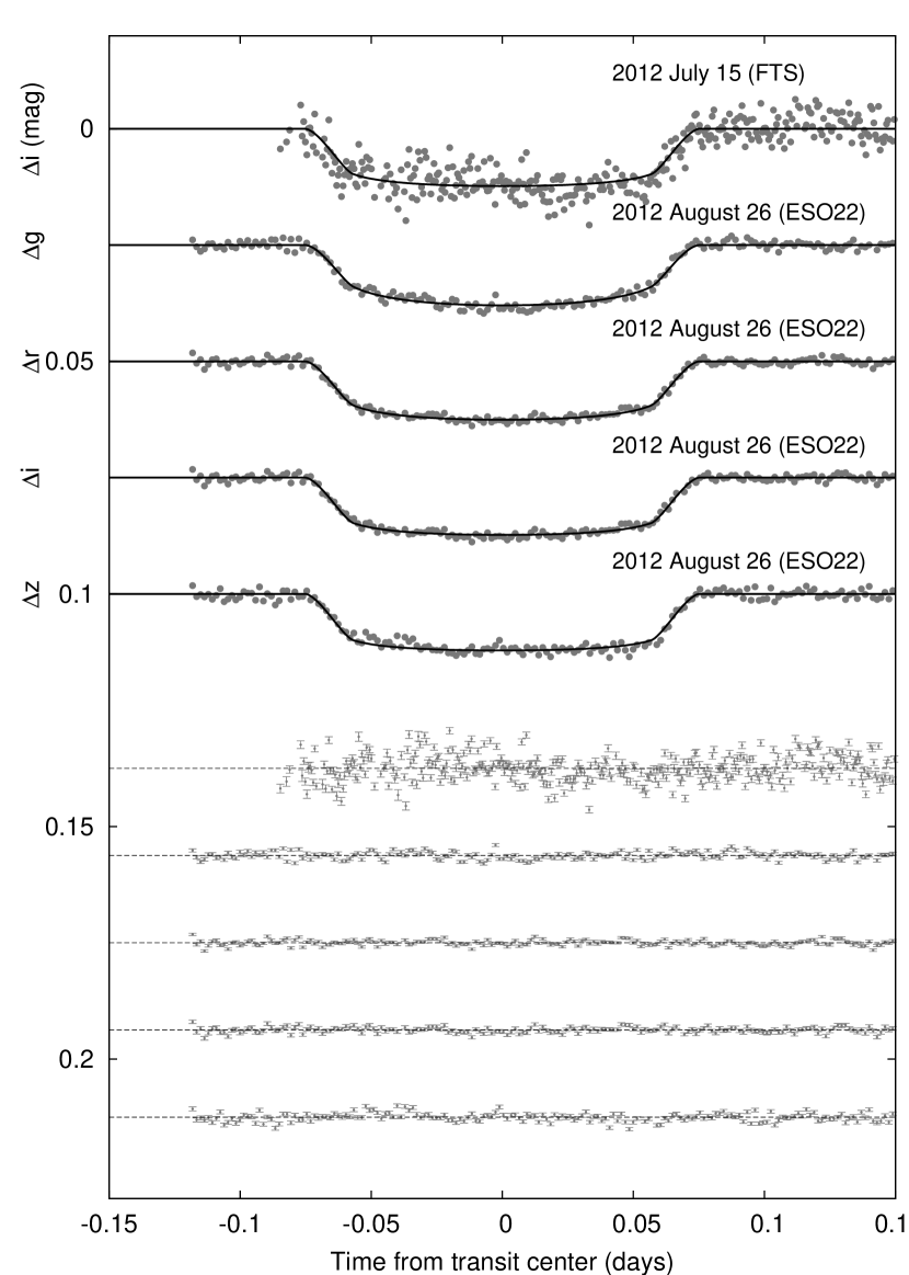
Figure 7.— Unbinned instrumental Sloan $g$-, $r$-, $i$- and $z$-band transit light curves of HATS-3. The dates and instruments used for each event are indicated. The light curves have been detrended using the EPD and TFA processes. Light curves are shifted for clarity. Our best fit is shown by the solid lines. Residuals from the fits are displayed at the bottom, in the same order as the top light curves.

Table 5Differential photometry of HATS-3

BJD	Mag	$\sigma_{\rm Mag}$	Mag(orig)	Filter	Instrument
(2 400 000$+$)
$55100.48159$	$-0.00404$	$0.00277$	$\cdots$	$r$	HS
$55366.57071$	$0.00091$	$0.00242$	$\cdots$	$r$	HS
$55334.64007$	$0.01110$	$0.00268$	$\cdots$	$r$	HS
$55359.47536$	$0.00753$	$0.00245$	$\cdots$	$r$	HS
$55391.40621$	$-0.00212$	$0.00256$	$\cdots$	$r$	HS
$55380.76328$	$-0.00029$	$0.00250$	$\cdots$	$r$	HS
$55437.52939$	$-0.00387$	$0.00252$	$\cdots$	$r$	HS
$55423.33825$	$0.00704$	$0.00250$	$\cdots$	$r$	HS
$55437.52985$	$0.00690$	$0.00425$	$\cdots$	$r$	HS
$55093.38841$	$0.00932$	$0.00260$	$\cdots$	$r$	HS

Note. — This table is available in a machine-readable form in the online journal. A portion is shown here for guidance regarding its form and content.

3. Analysis

3.1. Properties of the host star HATS-3

The stellar parameters of HATS-3, including $T_{\rm eff\star}$, $\log{g_{\star}}$, $\rm[Fe/H]$, and $v\sin{i}$ are derived from the high-resolution FEROS spectra. In a procedure similar to that presented in Mohler-Fischer et al. (2013), the thirteen spectra were analysed using the “Spectroscopy Made Easy” software package (SME; Valenti & Piskunov, 1996). The stellar parameters we list are the mean of the values derived from each spectrum, weighted by the signal-to-noise of the spectrum. The uncertainties in the stellar parameters are derived from the distribution of these parameters over the thirteen spectra.

Following the method described in Sozzetti et al. (2007) and applied in Penev et al. (2013), we determine fundamental stellar properties (mass, radius, age, and luminosity) based on the mean stellar density derived from the light curve fitting, the $T_{\rm eff\star}$ from the SME analysis, and the Yonsei-Yale (Y2; Yi et al., 2001) stellar evolution models. This analysis provides a value of $\log{g_{\star}}$=4.23$\pm$0.01, which is more precise than can be obtained via SME alone. We then fix this as the $\log{g_{\star}}$ for HATS-3 and repeat the SME analysis to determine the final stellar parameters listed in Table 6. The 1$\sigma$ and 2$\sigma$ confidence ellipsoids in $T_{\rm eff\star}$ and $a/R_{\star}$ are plotted in Figure 8, along with the Y2 isochrones for the SME determined $\rm[Fe/H]$, and a range of stellar ages. We find that HATS-3 is an F dwarf host, the first for the HATSouth survey, with $T_{\rm eff\star}$=$6351\pm 76$ K.

3.2. Excluding Blends

To rule out the possibility that HATS-3 is a blended stellar binary system that mimics the observable properties of a transiting planet system we conducted a blend analysis following the procedure described in Hartman et al. (2011). This procedure involves modelling the photometric light curves, photometry taken from public catalogs and calibrated to an absolute scale, and spectroscopically determined stellar atmospheric parameters. We compare the fits from a model consisting of a single planet transiting a star, to models of blended stellar systems with components having properties constrained by stellar evolution models.

We find that the single-star plus transiting planet model fits the data better than any non-planetary blend scenario. As is typically the case, there are some scenarios, in which the two brightest components in the blend are of similar mass, that we cannot rule out with greater than 5$\sigma$ confidence based on the photometry and atmospheric parameters. However, in all such cases there would be a secondary component in the blended object with a brightness that is $>38\%$ that of the primary star. That secondary component would itself be undergoing an orbit with a semiamplitude of several tens of km/s. Such a blend would have been easily detected, either as a double-lined spectrum, or via several $\rm km\,s^{-1}$ bisector-span variations.

3.3. Global Modeling of Data

In order to determine the physical planetary parameters, we carried out a joint, Markov-Chain Monte Carlo modelling of the HATSouth photometry, follow-up photometry, and the radial velocity measurements. The methodology is described fully in Bakos et al. (2010). The resulting planetary parameters are set out in Table 7. We list two sets of planet parameters: for the case of a circular orbit ($e=0$) and for the case that eccentricity is allowed to vary, whereby we get a best fit eccentricity of $e=0.25\pm 0.10$.

To estimate the significance of the non-zero eccentricity measurement we find that a Lucy & Sweeney (1971) test gives a non-negligible (7%) probability that the RV observations are consistent with a circular orbit, while the free-eccentricity and fixed-circular-orbit models yield nearly identical values for the Bayesian Information Criterion. We conclude that we cannot rule out a circular orbit based on the current RV observations.

Figure 8.— Model isochrones from Yi et al. (2001) for the measured metallicity of HATS-3, $\rm[Fe/H]$= $-0.157$, and ages of 0.2 Gyr (lowermost line), and 1 to 10 Gyr in 1 Gyr increments (left to right). The adopted values of $T_{\rm eff\star}$ and $a/R_{\star}$ are shown together with their 1$\sigma$ and 2$\sigma$ confidence ellipsoids. The open triangle shows the values from the initial SME iteration.

Table 6 Stellar parameters for HATS-3

Parameter	Value	Value	Source
	Circular	Eccentric
Spectroscopic properties
$T_{\rm eff\star}$ (K)	$6351\pm 76$	$6325\pm 83$	SME
$\rm[Fe/H]$	$-0.157\pm 0.07$	$-0.139\pm 0.09$	SME
$v\sin{i}$ ($\rm km\,s^{-1}$)	$9.12\pm 1.31$	$8.97\pm 1.8$	SME
Photometric properties
$V$ (mag)	$12.44\pm 0.2$	$12.44\pm 0.2$	APASS
$B$ (mag)	$12.46\pm 0.18$	$12.46\pm 0.18$	APASS
$J$ (mag)	$10.980\pm 0.021$	$10.980\pm 0.021$	2MASS
$H$ (mag)	$10.719\pm 0.024$	$10.719\pm 0.024$	2MASS
$K_{s}$ (mag)	$10.694\pm 0.021$	$10.694\pm 0.021$	2MASS
Derived properties
$M_{\star}$ ($M_{\sun}$)	$1.209\pm 0.036$	$1.300\pm 0.088$	YY+$a/R_{\star}$+SME
$R_{\star}$ ($R_{\sun}$)	$1.404\pm 0.030$	$1.725\pm 0.242$	YY+$a/R_{\star}$+SME
$\log{g_{\star}}$ (cgs)	$4.22\pm 0.01$	$4.08\pm 0.10$	YY+$a/R_{\star}$+SME
$L_{\star}$ ($L_{\sun}$)	$2.86\pm 0.21$	$4.28_{-1.02}^{+1.53}$	YY+$a/R_{\star}$+SME
$M_{V}$ (mag)	$3.62\pm 0.09$	$3.19\pm 0.31$	YY+$a/R_{\star}$+SME
$M_{K}$ (mag,ESO)	$2.46\pm 0.05$	$2.01\pm 0.30$	YY+$a/R_{\star}$+SME
Age (Gyr)	$3.2_{-0.4}^{+0.6}$	$3.1_{-0.4}^{+0.8}$	YY+$a/R_{\star}$+SME
Distance (pc)	$453\pm 11$	$556\pm 78$	YY+$a/R_{\star}$+SME
E(B-V)	$0.098\pm 0.054$	$0.096\pm 0.053$	YY+$a/R_{\star}$+SME

Table 7Orbital and planetary parameters

Parameter	Value	Value
	Circular	Eccentric
Light curve parameters
$P$ (days)	$3.547851\pm 0.000005$	$3.547849\pm 0.000005$
$T_{c}$ (${\rm BJD}$)	$2456155.96734\pm 0.00014$	$2456092.10547\pm 0.00039$
$T_{14}$ (days)	$0.1494\pm 0.0007$	$0.1486\pm 0.0011$
$T_{12}=T_{34}$ (days)	$0.0177\pm 0.0007$	$0.0175\pm 0.0007$
$a/R_{\star}$	$7.42\pm 0.12$	$6.18_{-0.64}^{+0.88}$
$\zeta/R_{\star}$	$15.16\pm 0.03$	$15.22_{-0.06}^{+0.11}$
$R_{p}/R_{\star}$	$0.1011\pm 0.0006$	$0.1010\pm 0.0005$
$b\equiv a\cos i/R_{\star}$	$0.497_{-0.027}^{+0.024}$	$0.489_{-0.029}^{+0.024}$
$i$ (deg)	$86.2\pm 0.3$	$84.3_{-2.0}^{+1.3}$
Limb-darkening coefficients
$a_{g}$ (linear term)	$0.4135$	$0.4160$
$b_{g}$ (quadratic term)	$0.3301$	$0.3286$
$a_{r}$	$0.2592$	$0.2607$
$b_{r}$	$0.3725$	$0.3721$
$a_{i}$	$0.1903$	$0.1915$
$b_{i}$	$0.3599$	$0.3597$
RV parameters
$K$ ($\rm m\,s^{-1}$)	$125.7\pm 15.7$	$131.7\pm 17.2$
$\sqrt{e}\cos\omega$	$\cdots$	$-0.355_{-0.089}^{+0.122}$
$\sqrt{e}\sin\omega$	$\cdots$	$0.356_{-0.252}^{+0.101}$
$e\cos\omega$	$\cdots$	$-0.176\pm 0.080$
$e\sin\omega$	$\cdots$	$0.175\pm 0.115$
$e$	$0$	$0.253\pm 0.110$
$\omega$	$\cdots$	$134\pm 25$
CORALIE RV jitter ($\rm m\,s^{-1}$)	$51.0$	$51.0$
FEROS RV jitter ($\rm m\,s^{-1}$)	$9.5$	$9.5$
CYCLOPS RV jitter ($\rm m\,s^{-1}$)	$65.0$	$65.0$
Planetary parameters
$M_{p}$ ($M_{\rm J}$)	$1.071\pm 0.136$	$1.138\pm 0.152$
$R_{p}$ ($R_{\rm J}$)	$1.381\pm 0.035$	$1.697\pm 0.238$
$C(M_{p},R_{p})$	$0.15$	$0.24$
$\rho_{p}$ ($\rm g\,cm^{-3}$)	$0.51\pm 0.07$	$0.28_{-0.08}^{+0.18}$
$\log g_{p}$ (cgs)	$3.14\pm 0.06$	$2.99\pm 0.12$
$a$ (AU)	$0.0485_{-0.0006}^{+0.0004}$	$0.0497\pm 0.0011$
$T_{\rm eq}$ (K)	$1648\pm 24$	$1816\pm 127$
$\Theta$	$0.062\pm 0.008$	$0.051_{-0.008}^{+0.012}$
$\langle F\rangle$ ($10^{9}$$\rm erg\,s^{-1}\,cm^{-2}$)	$1.66\pm 0.10$	$2.46_{-0.55}^{+0.90}$

4. Discussion

HATS-3b is the third planet to be discovered as part of the ongoing HATSouth survey for transiting exoplanets. Although it is the least massive of the three exoplanets with $M_{p}\approx 1.07$ $M_{\rm J}$, the host star is the most massive of the three host stars ($M_{\star}$=$1.21$ $M_{\sun}$).

When we allow the eccentricity to depart from e=0 in the global fit, we find a high eccentricity (e=$0.253\pm 0.110$) for HATS-3b. However like many planetary systems, the eccentricity is not well constrained by the radial velocity measurements, and more data will be required before this high eccentricity can be confirmed.

The $v\sin{i}$=$9.12\pm 1.31$ $\rm km\,s^{-1}$, combined with the large radius of the planet ($R_{p}=1.381\pm 0.035\,R_{\rm J}$) makes HATS-3b a prime target for follow-up Rossiter-McLaughlin monitoring to determine the spin-orbit alignment of the system. Interestingly with $T_{\rm eff\star}$=$6351\pm 76$ K this star lies just above the temperature of 6250 K which is noted as apparently marking a shift from aligned to misaligned hot Jupiters (Winn et al., 2010; Albrecht et al., 2012).

The power of the HATSouth network was illustrated in Penev et al. (2013) whereby three consecutive transits were detected at three different ground stations. For HATS-3b we show another aspect of the global network, which is that for much of the year observations from the sites give considerable overlap. Figure 9 shows that in pre-discovery a single transit of HATS-3b was simultaneously monitored by two different telescopes located over 8000 km apart on the Earth. This is testament to an active, homogeneous, global network.

There are 125 published transiting hot Jupiters (defined as $M_{p}>0.5\,M_{\rm J}$, $P<10\,d$) with both radius and mass precisely determined, so we can begin to plot the mass–radius diagram in terms of a density distribution of known exoplanets rather than just individual points. Such a plot is presented in Figure 10, with the position of HATS-3b marked in black with appropriate error bars. Interestingly, this diagram reveals an under-density of planets at 1.2–1.6 $M_{\rm J}$, even though there is no selection bias against detecting planets in this mass range with transit surveys. While it is possible that the gap is simply a feature of small number statistics, it further supports the case for expanding the sample of hot Jupiters to probe global trends in the populations.

Figure 9.— A single transit event from 2010 July 11 simultaneously observed from the HATSouth telescopes in Namibia (filled circles) and Chile (open squares). For two hours both telescopes were monitoring HATS-3b in-transit. Such simultaneous monitoring is possible for much of the year with the HATSouth network.

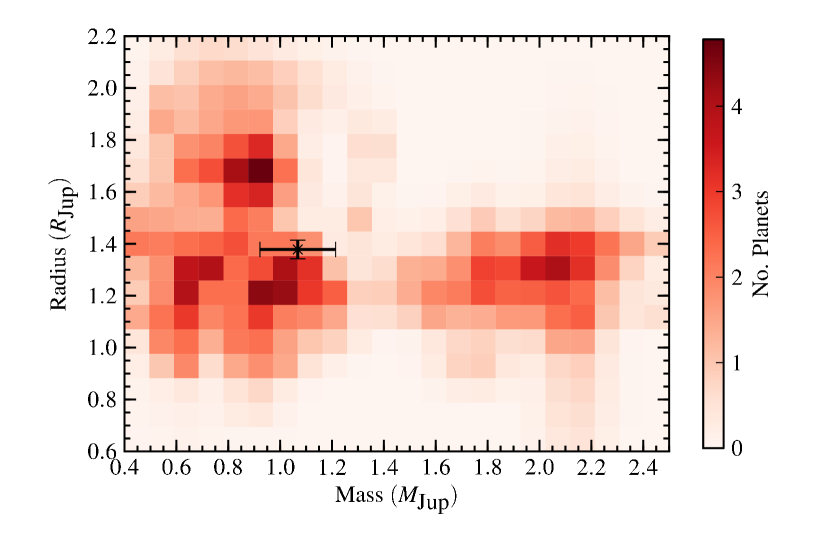
Figure 10.— A density plot showing the mass and radius for published transiting hot Jupiters, defined as planets with $M_{p}>0.5\,M_{\rm J}$ and $P<10\,d$. HATS-3b is plotted in black with appropriate uncertainties.

References

- Albrecht et al. (2012) Albrecht, S., Winn, J. N., Johnson, J. A., et al. 2012, ApJ, 757, 18
- Anderson et al. (2008) Anderson, D. R., Gillon, M., Hellier, C., et al. 2008, MNRAS, 387, L4
- Anderson et al. (2012) Anderson, D. R., Collier Cameron, A., Gillon, M., et al. 2012, MNRAS, 422, 1988
- Auvergne et al. (2009) Auvergne, M., Bodin, P., Boisnard, L., et al. 2009, A&A, 506, 411
- Bakos et al. (2004) Bakos, G., Noyes, R. W., Kovács, G., et al. 2004, PASP, 116, 266
- Bakos et al. (2010) Bakos, G. Á., Torres, G., Pál, A., et al. 2010, ApJ, 710, 1724
- Bakos et al. (2013) Bakos, G. Á., Csubry, Z., Penev, K., et al. 2013, PASP, 125, 154
- Bayliss & Sackett (2011) Bayliss, D. D. R., & Sackett, P. D. 2011, ApJ, 743, 103
- Bell et al. (1985) Bell, R. A., Edvardsson, B., & Gustafsson, B. 1985, MNRAS, 212, 497
- Berdyugina & Savanov (1994) Berdyugina, S. V., & Savanov, I. S. 1994, Astronomy Letters, 20, 755
- Bertin & Arnouts (1996) Bertin, E., & Arnouts, S. 1996, A&AS, 117, 393
- Bessell (1999) Bessell, M. S. 1999, PASP, 111, 1426
- Bessell (2007) —. 2007, PASP, 119, 605
- Borucki et al. (2010) Borucki, W. J., Koch, D., Basri, G., et al. 2010, Science, 327, 977
- Cardelli et al. (1989) Cardelli, J. A., Clayton, G. C., & Mathis, J. S. 1989, ApJ, 345, 245
- Charbonneau et al. (2002) Charbonneau, D., Brown, T. M., Noyes, R. W., & Gilliland, R. L. 2002, ApJ, 568, 377
- Claret (2004) Claret, A. 2004, A&A, 428, 1001
- de Medeiros et al. (2006) de Medeiros, J. R., Silva, J. R. P., Do Nascimento, Jr., J. D., et al. 2006, A&A, 458, 895
- Dopita et al. (2007) Dopita, M., Hart, J., McGregor, P., et al. 2007, Ap&SS, 310, 255
- Fressin et al. (2013) Fressin, F., Torres, G., Charbonneau, D., et al. 2013, ApJ, 766, 81
- Greiner et al. (2008) Greiner, J., Bornemann, W., Clemens, C., et al. 2008, PASP, 120, 405
- Gustafsson et al. (2008) Gustafsson, B., Edvardsson, B., Eriksson, K., et al. 2008, A&A, 486, 951
- Hamuy et al. (1992) Hamuy, M., Walker, A. R., Suntzeff, N. B., et al. 1992, PASP, 104, 533
- Hansen & Barman (2007) Hansen, B. M. S., & Barman, T. 2007, ApJ, 671, 861
- Hartman et al. (2011) Hartman, J. D., Bakos, G. Á., Torres, G., et al. 2011, ApJ, 742, 59
- Hellier et al. (2009) Hellier, C., Anderson, D. R., Gillon, M., et al. 2009, ApJ, 690, L89
- Hellier et al. (2010) Hellier, C., Anderson, D. R., Collier Cameron, A., et al. 2010, ApJ, 723, L60
- Ibata & Irwin (1997) Ibata, R. A., & Irwin, M. J. 1997, AJ, 113, 1865
- Kaufer & Pasquini (1998) Kaufer, A., & Pasquini, L. 1998, in Society of Photo-Optical Instrumentation Engineers (SPIE) Conference Series, Vol. 3355, Society of Photo-Optical Instrumentation Engineers (SPIE) Conference Series, ed. S. D’Odorico, 844–854
- Knutson et al. (2007) Knutson, H. A., Charbonneau, D., Allen, L. E., et al. 2007, Nature, 447, 183
- Kovács et al. (2005) Kovács, G., Bakos, G., & Noyes, R. W. 2005, MNRAS, 356, 557
- Kovács et al. (2002) Kovács, G., Zucker, S., & Mazeh, T. 2002, A&A, 391, 369
- Lucy & Sweeney (1971) Lucy, L. B., & Sweeney, M. A. 1971, AJ, 76, 544
- Mancini et al. (2013) Mancini, L., Nikolov, N., Southworth, J., et al. 2013, MNRAS, 430, 2932
- Mohler-Fischer et al. (2013) Mohler-Fischer, M., Mancini, L., Hartman, J. D., et al. 2013, ArXiv e-prints
- Nidever et al. (2002) Nidever, D. L., Marcy, G. W., Butler, R. P., Fischer, D. A., & Vogt, S. S. 2002, ApJS, 141, 503
- Penev et al. (2013) Penev, K., Bakos, G. Á., Bayliss, D., et al. 2013, AJ, 145, 5
- Pollacco et al. (2006) Pollacco, D. L., Skillen, I., Collier Cameron, A., et al. 2006, PASP, 118, 1407
- Queloz et al. (2000a) Queloz, D., Eggenberger, A., Mayor, M., et al. 2000a, A&A, 359, L13
- Queloz et al. (2000b) Queloz, D., Mayor, M., Weber, L., et al. 2000b, A&A, 354, 99
- Queloz et al. (2010) Queloz, D., Anderson, D., Collier Cameron, A., et al. 2010, A&A, 517, L1
- Robin et al. (2003) Robin, A. C., Reylé, C., Derrière, S., & Picaud, S. 2003, A&A, 409, 523
- Schlegel et al. (1998) Schlegel, D. J., Finkbeiner, D. P., & Davis, M. 1998, ApJ, 500, 525
- Southworth et al. (2009) Southworth, J., Hinse, T. C., Jørgensen, U. G., et al. 2009, MNRAS, 396, 1023
- Sozzetti et al. (2007) Sozzetti, A., Torres, G., Charbonneau, D., et al. 2007, ApJ, 664, 1190
- Stetson (1987) Stetson, P. B. 1987, PASP, 99, 191
- Valenti & Piskunov (1996) Valenti, J. A., & Piskunov, N. 1996, A&AS, 118, 595
- Wilson et al. (2008) Wilson, D. M., Gillon, M., Hellier, C., et al. 2008, ApJ, 675, L113
- Winn et al. (2010) Winn, J. N., Fabrycky, D., Albrecht, S., & Johnson, J. A. 2010, ApJ, 718, L145
- Yi et al. (2001) Yi, S., Demarque, P., Kim, Y.-C., et al. 2001, ApJS, 136, 417