A note on Rome-Southampton Renormalization with Smeared Gauge Fields.

Abstract

We have calculated continuum limit step scaling functions of bilinear and four-fermion operators renormalized in a Rome-Southampton scheme using various smearing prescriptions for the gauge field. Also, for the first time, we have calculated non-perturbative anomalous dimensions of operators renormalized in a Rome-Southampton scheme. The effect of such smearing first enters connected fermionic correlation functions via radiative corrections. We use off-shell renormalisation as a probe, and observe that the upper edge of the Rome-Southampton window is reduced by link smearing. This can be interpreted as arising due to the fermions decoupling from the high momentum gluons and we observe that the running of operators with the scale at large lattice momenta shows enhanced lattice artefacts. We find that the effect is greater for HEX smearing than for Stout smearing, but that in both cases additional care must be taken when using off-shell renormalisation with smeared gauge fields compared to thin link simulations.

I Introduction

Link smearing is a popular method in lattice QCD, and is simple to combine with any fermion action. Certain smearing types are differentiable, e.g. Stout Morningstar:2003gk and HEX Capitani:2006ni , and can therefore be used in the calculation of the fermionic force term in hybrid Monte Carlo. For staggered fermions, smearing has been motivated as suppressing taste breaking by reducing gluon exchanges of momenta $\sim\pi/a$ Orginos:1999cr . Smearing improves the behaviour of lattice perturbation theory by making the tadpole contribution vanishingly small Bernard:1999kc . Smearing with Wilson fermions has been very successful in reducing chiral symmetry breaking errors by suppressing dislocations that lead to eigenvalues below $m^{2}$ of $H_{W}^{2}$, ($H_{W}$ is the hermitian Wilson-Dirac operator $H_{W}=\gamma_{5}(D_{W}+m)$ with $D_{W}$ the Wilson-Dirac operator and $m$ the quark mass), Hasenfratz:2007rf . This allows smaller masses to be simulated on coarser lattices without exceptional configurations.

Small eigenvalues of $\gamma_{5}(D_{W}-M)$ are responsible for residual chiral symmetry breaking in domain wall fermions at finite $L_{s}$, the size of the fifth dimension Antonio:2008zz . This manifests itself in simulations as the residual mass $m_{res}$. By reducing the number of modes in the region where the domain wall fermion’s ‘tanh’ approximation to the sign function is most inaccurate it is hoped that one could obtain small $m_{res}$ without increasing $L_{s}$.

By suppressing the low modes we are simultaneously improving the condition number of the Dirac operator. Thus smearing should also help by speeding up matrix inversions, as has already been observed for the overlap operator Hasenfratz:2007rf .

One might worry that decoupling the fermion sector from the QCD gluodynamics at a scale below the lattice cut off might carry some penalty, and it is prudent to carefully check the effects of this. For some time it has been known that quantities like the static potential at short distances Hasenfratz:2001hp are strongly distorted by smearing. In the case of the static potential the distortion occurs for distances $r$ with $\frac{r}{a}<2$, where lattice artefacts are large anyway. It is also known that link smearing drives the renormalization constants towards their tree level valuesKurth:2010yk .

The Rome-Southampton method for non-perturbative renormalization (NPR) Martinelli:1994ty is widely used. Steady improvements to the original method: momentum sources Gockeler:1998ye , non-exceptional momenta Aoki:2007xm and twisted boundary conditions Arthur:2010ht , have led to a precise method for renormalizing in lattice calculations (see Aoki:2010pe for example). The remaining systematic error is dominated by a perturbative matching between the intermediate scheme, such as the RI/MOM, and the $\overline{MS}$ scheme, which is done at a scale accessible by current lattice calculations. The perturbative conversion error can be reduced by increasing the matching scale. The available lattice momentum scale, $\frac{\pi}{a}$, can be of the order $3\text{ GeV}$ to $5\text{ GeV}$ which is high enough to reduce the matching error significantly. A method has been developed Arthur:2010ht (see also Durr:2010aw ) that uses multiple lattices to stay below the lattice cut-off at all stages of the calculation and calculate non-perturbative renormalization constants at high energies where the effects of low energy QCD are minimised and perturbation theory gives a good description of the running, which should make it possible to reduce the error even further in the future. Link smearing and non-perturbative renormalization have often been used together to predict quantities of great phenomenological importance, e.g. in recent calculations of the kaon bag parameter $B_{K}$ Aubin:2009jh ; Durr:2011ap .

Rome-Southampton vertex functions may also be a case where the short distance properties are of crucial importance, especially since momentum scales close to the lattice cut-off are important. In this paper we perform a systematic study of the effects of smearing on the high momentum behaviour of NPR vertex functions and compare to the unsmeared “thin link” case. The continuum limit is taken at all stages assuming an $O(a^{2})$ scaling violation and results are compared in the continuum limit where universality should be satisfied.

We aim to check how link smearing would affect the program of Rome-Southampton renormalization that has been used for kaon physics simulations in the RBC/UKQCD collaboration. The results should be of interest for non-perturbative renormalization with any action since we will extrapolate smeared and unsmeared data to the continuum. The crucial point in all that follows is that the continuum limit results should be independent of the details of the intermediate lattice calculations, in particular if smeared links have been used or not.

In section II we calculate the smearing form factor and the associated smearing radius non-perturbatively. Section III describes our method of computing step scaling functions and anomalous dimensions from NPR vertex functions and extrapolating to vanishing lattice spacing. The calculation of anomalous dimensions in a Rome-Southampton scheme is a new method introduced in this paper. Section IV shows NPR vertex functions calculated using different smearing prescriptions, and derives step scaling functions and anomalous dimensions from them. Finally we conclude in section V and comment on the use of smeared links together with Rome-Southampton renormalization.

In this work we have not generated gauge fields using a smeared action; in order for direct comparison we calculate the relevant vertex functions on the same gauge ensembles with different smearing parameters. For the gauge ensembles we use those of the RBC/UKQCD collaboration, Allton:2008pn ; Aoki:2010dy . They are generated using the Iwasaki gauge action and thin-link domain-wall fermions at lattice spacings $a^{-1}=1.73(3)\text{ GeV}$ on a $24^{3}\times 64\times 16$ volume and $a^{-1}=2.28(3)\text{ GeV}$ on a $32^{3}\times 64\times 16$ volume, that we refer to as the coarse and fine lattices respectively. The bare quark masses available on the coarse lattice are $am={0.005,0.01,0.02}$ with $m_{res}=0.00315(4)$ and on the fine lattice $am={0.004,0.006,0.008}$, $m_{res}=0.000666(8)$.

II Effect of Smearing on the Gauge Field

The effect of smearing on the lattice Feynman rules is to introduce a form factor in the quark-gluon vertex Bernard:1999kc . After applying $n$ steps of smearing to obtain the gauge link $V^{(n)}_{\mu}(x+a\hat{\mu}/2)$ we can define a gauge field through

$$V^{(n)}_{\mu}(x+a\hat{\mu}/2)=\exp(iaA^{(n)}_{\mu}(x+a\hat{\mu}/2)).$$ (1)

At leading order, the smeared and unsmeared gauge fields are related by,

$$A^{(1)}_{\mu}(x+a\hat{\mu}/2)=\sum_{y,\nu}h_{\mu\nu}(y+a\hat{\nu}/2)A^{(0)}_{\nu}(x+a\hat{\mu}/2+y+a\hat{\nu}/2).$$ (2)

with the momentum space the form factor $h_{\mu\nu}$,

$$h_{\mu\nu}(q) = f^{(1)}(q)\left(\delta(q)-\frac{q_{\mu}q_{\nu}}{q^{2}}\right)+\frac{q_{\mu}q_{\nu}}{q^{2}},$$ (3)

$q_{\mu}=\frac{2}{a}\sin\left(\frac{aq_{\mu}}{2}\right)$. Applying the smearing transformation $n$ times changes $f^{(1)}(q)$ to $f^{(n)}(q)=(f^{(1)}(q))^{n}$.

The form factor $f^{(n)}(q)$ is Capitani:2006ni ,

$$f^{(n)}(q)=\left[1-\frac{\alpha}{2(d-1)}q^{2}\right]^{n}$$ (4)

for APE smearing with parameter $\alpha$ in $d$ dimensions. Stout has the same form. For HYP and HEX $\alpha q^{2}$ should be replaced by $\alpha_{1}\Omega_{\mu\nu}p^{2}_{\nu}$, where $\Omega_{\mu\nu}=\left(1+\alpha_{2}(1+\alpha_{3})\right)\delta_{\mu\nu}$ to lowest order in $q^{2}$. For small $q^{2}$ we can write the term in brackets as an exponential

$$f^{(n)}(q)=\exp\left(-\frac{n\alpha}{2(d-1)}q^{2}\right)+O((q^{2})^{2}),$$ (5)

and identify the mean square radius,

$$\langle r^{2}\rangle=\frac{n\alpha}{(d-1)},$$ (6)

as a measure of the space-time region affected by the smearing transformation, in most practical simulations this radius is of the order one. This new distance scale introduced by smearing could alter the high energy behaviour of the theory. In particular, since NPR directly probes radiative loop corrections it may be highly sensitive to this new scale.

We fix the gauge fields to the Landau gauge and then smear them using different smearing types: Stout, HYP and HEX. HYP smearing is described in Hasenfratz:2001hp and HEX in Capitani:2006ni . Both use the same hypercubic blocking transformation but HEX uses the STOUT projection to $SU(3)$ and HYP uses the APE projection. HYP and HEX smearing require the specification of three parameters, $(\alpha_{1},\alpha_{2},\alpha_{3})$ which we choose as $\{0.75,0.60,0.30\}$ for HYP (this is sometimes called HYP-1) and $\{0.95,0.76,0.38\}$ for HEX. We show results using one and two hits of HYP smearing and two hits of HEX smearing. We also show three hits of Stout with parameter $\alpha_{1}=0.1$, using the convention of Morningstar:2003gk . Using Appendix A of Capitani:2006ni we can therefore calculate the tree level values of $\langle r^{2}\rangle$, which we give in the first row of Table 1. The values in this table are small, indicating the effect of smearing hardly extends beyond one lattice spacing.

It is possible to calculate the quantity $f^{(n)}(q)$ defined in equation (4) non-perturbatively as follows. Due to the Landau gauge fixing, the equation $q_{\mu}A^{(0)}_{\mu}=0$ holds to high precision. From equation (3) this means,

$$A^{(n)}_{\mu}(q)=f^{(n)}(q)A^{(0)}_{\mu}(q),$$ (7)

and hence

$$f^{(n)}(q)=\left(\frac{\textrm{Tr}[A^{(n)}_{\mu}(q)A^{(n)}_{\mu}(-q)]}{\textrm{Tr}[A^{(0)}_{\mu}(q)A^{(0)}_{\mu}(-q)]}\right)^{1/2}.$$ (8)

The lattice gluon field is defined by,

$$A_{\mu}(x+a\hat{\mu}/2)=\frac{1}{2ia}\Bigl{(}\left[U_{\mu}(x+a\hat{\mu}/2)-U^{\dagger}_{\mu}(x+a\hat{\mu}/2)\right]\\ -\frac{1}{N_{c}}\textrm{Tr}\left[U_{\mu}(x+a\hat{\mu}/2)-U^{\dagger}_{\mu}(x+a\hat{\mu}/2)\right]I_{N_{C}\times N_{C}}\Bigr{)},$$ (9)

and in momentum space by,

$$A_{\mu}(q)=e^{i\frac{q_{\mu}}{2}}\sum_{x}e^{iq\cdot{x}}A_{\mu}(x+a\hat{\mu}/2).$$ (10)

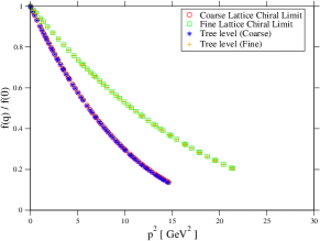
(a) 3 STOUT $f^{(3)}(q)$ weak field

(b) 3 STOUT $f^{(3)}(q)$ full field

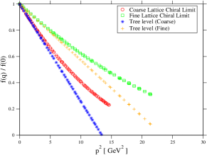
(c) 1 HYP $f^{(1)}(q)$ weak field

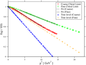
(d) 1 HYP $f^{(1)}(q)$ full field

Figure 1: $f^{(n)}(q)$ measured on the coarse (red) and fine (green) ensembles for three hits of Stout, (a) and (b), and one of HYP, (c) and (d). On the left are results using a weak field as a cross check for results on the right using the full field. Perturbative predictions in blue and orange. Fits are to a quadratic in $q^{2}$ over the indicated range.

(a) 2 HYP $f^{(2)}(q)$ weak field

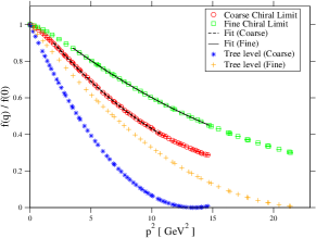
(b) 2 HYP $f^{(2)}(q)$ full field

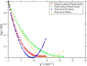
(c) 2 HEX $f^{(2)}(q)$ weak field

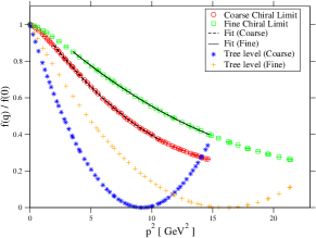
(d) 2 HEX $f^{(2)}(q)$ full field

Figure 2: $f^{(n)}(q)$ measured on the coarse (red) and fine (green) ensembles for two hits of HYP, (a) and (b), and two of HEX, (c) and (d). On the left are results using a weak field as a cross check for results on the right using the full field. Perturbative predictions in blue and orange. Fits are to a quadratic in $q^{2}$ over the indicated range.

This can be used in equation (8) and $f\left(q\right)$ calculated for different levels of smearing. In the left column of Figures 1 and 2, (a cylinder cut in momentum space Leinweber:1998im of width $\frac{2\pi}{L_{i}}$, $i$ is the spatial lattice index, has been used) are the ‘weak field’ results. This is introduced to check the analysis against perturbation theory. Namely, we multiply every gauge field $A_{\mu}$ by $10^{-3}$, generate $U_{\mu}$ by exact exponentiation and then apply the smearing. For this artificially produced weak field we find good agreement with the perturbative expectation, as shown in the left column of Figures 1 and 2. The ‘full field’ results, using the original, unreduced $U_{\mu}$, are shown on the right.

The identification of the quantity $\sqrt{\langle r^{2}\rangle}$ as an effective smearing radius assumes a Gaussian profile for $f^{(n)}(q)$. From the plots of $f^{(n)}(q)$ it is clear that it is not Gaussian and fitting the curves with a Gaussian fails. We attempt to extract a value of $\langle r^{2}\rangle$ in two ways: (a) using the point where $f^{(n)}(q)$ is equal to $e^{-1/2}$ of its initial value to define a scale,

$$\langle r^{2}\rangle=\frac{1}{q^{2}}\Big{|}_{f^{(n)}(q)/f^{(n)}(0)=e^{-1/2}}$$ (11)

(b) assuming that the functional form of $f^{(n)}(q)$ is the same as at tree level,

$$f^{(n)}(q)=\left(1-\frac{1}{2n}\langle r^{2}\rangle q^{2}\right)^{n}=1-\frac{1}{2}\langle r^{2}\rangle q^{2}+cq^{4}+O(q^{6}),$$ (12)

and fitting to a quadratic, then obtaining $\langle r^{2}\rangle$ from the linear co-efficient. The results of both of these strategies are given in Table 1.

These results are far from the perturbative picture, giving significantly smaller radii. In order to make the identification of the perturbative function $f^{(n)}(q)$ in equation (3) with equation (8) we assume that equation (2) is valid. However this is only the case up to leading order in $a$, the smeared gauge fields do not even satisfy the Landau condition. Our calculation of $f^{(n)}(q)$ is the first time this has been measured non-perturbatively and gives unexpectedly small smearing radii.

Having seen how smearing affects the high momentum part of the gauge field we turn to the main focus of this paper: how smearing affects NPR at high scales.

Smearing		3 Stout	1 HYP	2 HYP	2 HEX
$\sqrt{\langle r^{2}\rangle}$	tree level	0.667	0.775	0.943	1.139
	coarse ensemble (exp)	0.5307(4)	0.5418(3)	0.6847(5)	0.7165(4)
	coarse ensemble (fit)	0.509(2)	0.514(2)	0.705(1)	0.746(2)
	fine ensemble (exp)	0.5625(2)	0.5663(2)	0.7271(2)	0.7730(3)
	fine ensemble (fit)	0.543(1)	0.540(1)	0.747(1)	0.802(1)

Table 1: Effective smearing radius in lattice units measured using equation (11); (exp) and equation (12); (fit). The disagreement between the two definitions arises because the curves are not really Gaussian.

III Renormalization and Running of Lattice Operators

Following Arthur:2010ht we calculate step scaling functions in the continuum limit for a variety of operators. After obtaining the Fourier transformed propagator $S(z,p)$ by solving

$$\sum_{z}D(x,z)S(z,p)=e^{ipx},$$ (13)

we multiply by a phase to get $S^{\prime}(z,p)=e^{-ipz}S(z,p)$ and calculate the Green function for the bilinear operator $O_{\Gamma}(z)=\bar{q}(z)\Gamma q(z)$

$$\langle G_{\cal{}_{O}}(p_{1},p_{2})\rangle=\langle\frac{1}{V}\sum_{z}\gamma_{5}(S^{\prime}(z,p_{1}))^{\dagger}\gamma_{5}\Gamma S^{\prime}(z,p_{2})\rangle.$$ (14)

We use the inverse propagator, $S^{-1}(p)$, to make the amputated vertex function,

$$\Pi_{{\cal O}}(p)=\langle S^{-1}(p_{1})\rangle\langle G_{{\cal{}_{O}}}(p_{1},p_{2})\rangle\langle S^{-1}(p_{2})\rangle.$$ (15)

For details on the procedure for the renormalization of $B_{K}$ see Aoki:2010pe . Only non-exceptional momenta; $p_{\mu}$, $q_{\mu}$, $r_{\mu}$ where $r_{\mu}=p_{\mu}-q_{\mu}$ and $p^{2}=q^{2}=(p-q)^{2}$ are used. To access momenta that are not Fourier modes we solve equation (13) using twisted boundary conditions. The momenta in the direction $\mu$ are then modified such that $p_{\mu}$ becomes $p_{\mu}+\frac{\pi\theta_{\mu}}{L_{\mu}}$, where $L_{\mu}$ is the extent of the lattice in that direction and $\theta_{\mu}$ the $\mu$ component of a vector parallel $p$. We keep the directions of $p_{\mu}$, $q_{\mu}$ and $r_{\mu}$ fixed and use different twists ($\theta$s) to vary their magnitudes. In this way we avoid ${\cal H}(4)$ breaking artefacts Arthur:2010ht .

We define the normalized trace of the amputated vertex function with a projector $\mathbf{P}_{{\cal{}_{O}}}$ as,

$$\Lambda_{{\cal{}_{O}}}(\mu,a,m)=\frac{1}{12}Tr\left[\mathbf{P}_{{\cal{}_{O}}}\Pi_{{\cal{}_{O}}}(p,a,m)\right]_{p^{2}=\mu^{2}},$$ (16)

where the $\mathbf{P}_{{\cal{}_{O}}}$ is chosen to project out a desired gamma matrix structure and to give a normalization such that $\Lambda_{\cal O}$ is unity at tree level. The trace is over spinor and color degrees of freedom. The renormalized amputated vertex functions of bilinears are related to the bare ones by

$$\Lambda_{{\cal{}_{O}},R}(\mu,a,m)=\frac{Z_{{\cal{}_{O}}}(\mu,a,m)}{Z_{q}}\Lambda_{{\cal{}_{O}}}(\mu,a,m),$$ (17)

the $Z_{q}$ factor comes from the inverse propagators required for the external leg amputation. The Rome-Southampton renormalization condition on the projected vertex functions is,

$$\lim_{m\to 0}\Lambda_{{\cal{}_{O}}R}(\mu,a,m)=1.$$ (18)

To look at the running of each operator individually we have to remove the factors of $Z_{q}$ implicit in $\Lambda_{{\cal{}_{O}}}$. Dividing by the axial vertex $\Lambda_{A}$

$$R_{{\cal O}}(\mu,a,m)=\frac{\Lambda_{A}(\mu,a,m)}{\Lambda_{\cal O}(\mu,a,m)}=\frac{Z_{{\cal O}}(\mu,a,m)}{Z_{A}}$$ (19)

accomplishes this since $Z_{A}$ is fixed by current conservation and does not run with $\mu$. These quantities are extrapolated to the chiral limit to give the renormalization constant,

$$Z_{{\cal O}}(\mu,a)=Z_{A}\lim_{m\to 0}R_{\cal O}(\mu,a,m).$$ (20)

We introduce a ratio of the $R_{\cal O}$s at different $\mu$,

$$\Sigma_{\cal O}(\mu,s\mu,a)=\lim_{m\to 0}\frac{R_{\cal O}(s\mu,a,m)}{R_{\cal O}(\mu,a,m)},$$ (21)

which has,

$$\sigma_{\cal O}(\mu,s\mu)=\lim_{a\to 0}\Sigma_{\cal O}(\mu,s\mu,a)=\frac{Z_{\cal O}(s\mu)}{Z_{\cal O}(\mu)}$$ (22)

as its continuum limit and is called the step scaling function. This is the factor required to change the scale from $\mu$ to $s\mu$. Because we take the continuum limit the final step scaling functions should be action independent. To obtain the mass step scaling function we use the pseudoscalar bilinear operator ${\cal O}=\bar{q}\gamma_{5}q$. For the quark field renormalization we use the vector bilinear ${\cal O}=\bar{q}\gamma_{\mu}q$ and for the tensor current we use ${\cal O}=\bar{q}\sigma_{\mu\nu}q$. The renormalization of $B_{K}$ requires the VV+AA four quark operator $\left(\bar{q}\gamma_{\mu}q\right)\left(\bar{q}\gamma_{\mu}q\right)+\left(\bar{q}\gamma_{5}\gamma_{\mu}q\right)\left(\bar{q}\gamma_{5}\gamma_{\mu}q\right).$

In order to cleanly separate high and low energy behaviour it is useful to have a function that depends on only one scale. This is given by the anomalous dimension $\gamma_{\cal O}$,

$$\sigma_{\cal O}(\mu,s\mu)=\exp\left(\int_{\alpha_{1}}^{\alpha_{2}}\frac{\gamma_{\cal O}(\alpha)}{\beta(\alpha)}d\alpha\right)\\ =\exp\left(\int_{\mu_{1}}^{\mu_{2}}\frac{\gamma_{\cal O}(\mu)}{\mu}d\mu\right)$$ (23)

using the chain rule. With $\mu_{1}=\mu$ and $\mu_{2}=(1+\epsilon)\mu$ for small $\epsilon$ the right hand side becomes,

$$\sigma_{\cal O}\left(\mu,(1+\epsilon)\mu\right)\approx\exp\left(\epsilon\gamma_{\cal O}(\mu)\right)\\ \rightarrow\gamma_{\cal O}(\mu)\approx\ln\left(\sigma_{\cal O}(\mu,(1+\epsilon)\mu)\right)/\epsilon.$$ (24)

As we will see, the vertex function data, and hence the step scaling functions derived from it, are very smooth functions of the scale which means they can be differentiated as above without difficulty.

IV Results

IV.1 Vertex Functions

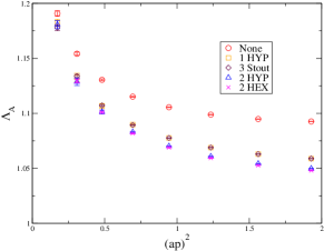
(a) $\Lambda_{\cal A}$, $RI-SMOM$

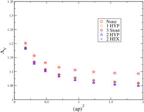
(b) $\Lambda_{\cal V}$, $RI-SMOM$

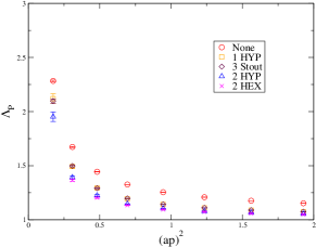
(c) $\Lambda_{\cal P}$, $RI-SMOM$

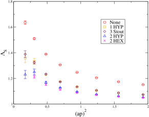
(d) $\Lambda_{\cal S}$, $RI-SMOM$

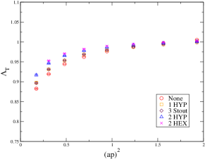
(e) $\Lambda_{\cal T}$, $RI-SMOM$

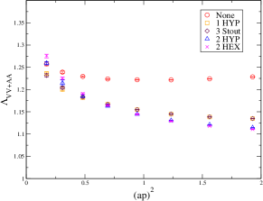
(f) $\Lambda_{\cal VV+AA}$, $RI-SMOM(\cancel{q},\cancel{q})$

Figure 3: Amputated projected vertex functions in the RI-SMOM scheme, see Sturm:2009kb for details of this scheme and the relevant projectors. The smearing used is indicated in the figure labels. Smearing is seen to drive the renormalization constants closer to their tree level values and thus the projected vertex is driven closer to one.

In Figure 3 we show the vertex functions calculated on the $32^{3}$ lattice with valence and sea quark masses equal to $0.004$ in lattice units. We are showing this ensemble, as it is closest to the chiral and continuum limit, but other ensembles show similar results. The momentum definition $p_{\mu}=\frac{2\pi n_{\mu}+\pi\theta_{\mu}}{L_{\mu}}$ is used rather than another possible definition $\bar{p}_{\mu}=\frac{1}{a}\sin(ap_{\mu})$. Here $n_{\mu}$ is a vector of integers and $\theta_{\mu}$ a vector parallel to $n_{\mu}$. Explicitly, $p_{\mu}$ is parallel to $(0,1,1,0)$ and $q_{\mu}$ is parallel to $(-1,0,1,0)$, the twist added to $p_{\mu}$ is $(0,\theta,\theta,0)$ and that added to $q_{\mu}$ is $(-\theta,0,\theta,0)$ where $\theta$ is varied to vary the magnitude of the momentum. The definition using $\sin$ agrees at low momenta but gives smaller values at higher momentum for the same Fourier mode $n_{\mu}$ and twist $\theta_{\mu}$. In Figure 3 the unsmeared vertex functions are shown along with the same quantity computed using four different types of smearing. The effect of smearing is to bring the configurations closer to the free field. Thus the renormalization constants are driven closer to their tree level values and, because of how the projector is defined, the vertex functions are driven closer to one.

IV.2 Step Scaling Functions

The renormalization constant computed on a smeared gauge field should be combined with its corresponding operator expectation value, also evaluated on a smeared background and that combination extrapolated to the continuum limit. In the continuum limit all trace of the lattice formulation, and hence of any smearing prescription, should vanish. To observe this we take ratios of renormalization constants at different scales and calculate $\sigma(\mu,s\mu)$ in equation (22). The step scaling function $\sigma$ is scheme dependent. For the bilinear vertices there are two choices of (non-exceptional) scheme, called SMOM and $\text{SMOM}_{\gamma_{\mu}}$ which can be used. For $B_{K}$ there are four non-exceptional schemes (see Sturm:2009kb and Aoki:2010pe for definitions of the schemes). We show results in the schemes where the unsmeared data has been found to agree best with perturbation theory. The four quantities and the scheme we use are given in table 2.

Step scaling function	Scheme
$\sigma_{Z_{m}}$	SMOM
$\sigma_{Z_{q}}$	$\text{SMOM}_{\gamma_{\mu}}$
$\sigma_{Z_{T}}$	$\text{SMOM}_{\gamma_{\mu}}$
$\sigma_{Z_{B_{K}}}$	$\text{SMOM}_{\cancel{q},\cancel{q}}$

Table 2: The schemes in which each step scaling function is calculated.

No attempt to account for the systematic errors due to spontaneous chiral symmetry breaking or other sources is made since these are small, Aoki:2010dy , and should affect smeared and unsmeared data to roughly the same degree.

Since we do not have perfectly matched momentum values $p^{2}$ between the two available lattices, we first interpolate the lattice data in $(ap)^{2}$ and then choose several values of $p^{2}$ at which the continuum limit is taken linearly in $a^{2}$. We use the ansatz,

$$\frac{c_{-3}}{(ap)^{6}}+\sum_{i=0}^{2}\frac{c_{-i}}{(ap)^{2i}}+c_{1}(ap)^{2}.$$ (25)

This functional form is motivated by the $\frac{1}{p^{6}}$ behaviour observed at low momenta in non-exceptional vertex functions Aoki:2007xm together with the leading finite lattice spacing error which for the chirally improved fermion formulation we use are $O(a^{2})$. There is also the intrinsic running of the operator itself, which we account for with a polynomial in $\frac{1}{(ap)}$. With this ansatz we fit only the data that are in the range of momenta we are investigating and these fits are used in all that follows. Chiral extrapolations are performed linearly in $am$ to $-am_{res}$ and are very benign Arthur:2010ht . Continuum extrapolations are obtained from a linear ‘fit’ in $a^{2}$ using two different lattices. Because our fermion action, domain wall, is chiral all quantities are automatically off-shell $O(a)$ improved. There is also an $O(am_{res})$ effect but as $m_{res}$ is of order $10^{-3}$ this can be safely neglected. Using two lattice spacings lets us account for the leading $O(a^{2})$ error. Only $O(a^{4})$ and higher terms remain untreated, which should be small for sufficiently low $(ap)^{2}$, lying within the Rome-Southampton scaling window. This means that continuum extrapolations with domain wall fermions, or other chirally improved actions, using a smaller number of lattice spacings can be as robust as using more lattice spacings but an unimproved fermion formulation since the leading non-removed error is the critical quantity. The detailed range of this window may, however, depend on the smearing prescription, and if $O(a^{4})$ and higher terms become significant they would manifest themselves as incorrect removal of lattice artefacts in our simple $a^{2}$ continuum extrapolation.

We have chosen to focus on the two differentiable varieties of smearing, Stout and HEX, because of their usefulness in HMC. We plot the step scaling function of the mass from a fixed low scale, $1.4\text{ GeV}$, to a high scale that varies in the range $(1.4\text{ GeV},3.0\text{ GeV})$ in figure 4. The value $1.4\text{ GeV}$ is chosen to match the choice of scale in :2012opa . In each panel the red data is the step scaling function on the coarse lattice, the green data is on the fine lattice and the blue data uses these two to extrapolate in $a^{2}$ to vanishing lattice spacing. Each of the points in the figure is an arbitrary scale we have interpolated to and performed the extrapolation at. The different panels show the three different smearing prescriptions (a) no smearing, (b) 3 hits of stout smearing and (c) 2 hits of HEX smearing. It is evident that the anomalous running at finite lattice spacing for the smeared is much weaker than in the unsmeared case. The smearing irons out the ultraviolet fluctuations leading to a prediction of little to no anomalous running at higher momenta. It is in this sense that we find it is perhaps more accurate to describe smeared gauge fields as closer to the trivial configuration than as closer to continuum QCD.

This is not necessarily a problem per se, providing the effects are well described by only $O(a^{2})$ errors such that we can successfully extrapolate to a universal continuum limit. If it is the case that we can continuum extrapolate away any difference between the smeared and unsmeared data then the blue curves in all three figures should be identical. This can be seen more clearly when all three continuum limits $\sigma_{m}$ are overlayed in Figure 5(a). We also display the same analysis for $\sigma_{q}$, $\sigma_{T}$, and $\sigma_{Z_{B_{K}}}$. Here, we see a universal slope for the continuum step-scaling function in the region $1.4$ GeV to $1.7$ GeV. However, we find that the smeared approaches have sufficiently large lattice artefacts to disagree with the thin link running in the continuum limit (taken using purely $O(a^{2})$ extrapolation) when the physical momenta exceed around $1.75$ GeV for the HEX smeared case and around $2.0$ GeV for the stout smeared case. We interpret this as indicating that radiative corrections in smeared link simulations possess a second, hidden, lattice spacing defined by the smearing radius that can pinch the Rome-Southampton scaling window compared to thin link simulations.

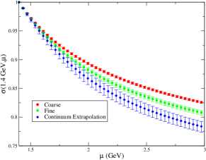
(a) $\sigma_{Z_{m}}(1.4\text{ GeV},\mu)$, no smearing

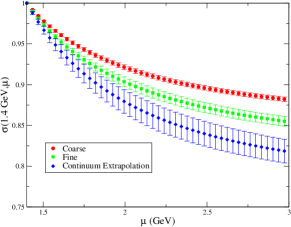
(b) $\sigma_{Z_{m}}(1.4\text{ GeV},\mu)$, 3 stout

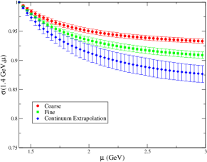
(c) $\sigma_{Z_{m}}(1.4\text{ GeV},\mu)$, 2 HEX

Figure 4: The step scaling function for $Z_{m}$ extrapolated to the continuum in the SMOM scheme. (a) in unsmeared (b) uses 3 steps of stout smearing (c) uses 2 steps of HEX smearing.

In Figure 6(a) we show the anomalous dimension of the mass from $1\text{ GeV}$ up to $3\text{ GeV}$ using two different smearings compared to unsmeared data. The anomalous dimension plots show the effects of smearing more clearly, up to a scale of the order $1.75\text{ GeV}$ all three anomalous dimensions agree with each other. After this the three start to diverge strongly. The solid black line is the perturbative result for this scheme,

$$\gamma_{O}(\mu)=-\sum_{i}\gamma_{O,i}\left(\frac{\alpha_{s}(\mu)}{4\pi}\right)^{i}$$ (26)

where the co-efficients for $\gamma_{m}$ and $\gamma_{q}$ are obtained from Almeida:2010ns those for $\gamma_{T}$ from Sturm:2009kb and for $\gamma_{BK}$ from Aoki:2010pe and $\alpha_{s}$ is in the $\overline{MS}$ scheme. The highest number of loops available (two for $B_{K}$ and the tensor, three for the mass and quark field) is used for the perturbative line. For $\alpha_{s}$ we use $\alpha_{s}(m_{Z})=0.1184$ and run down to $m_{b}$ with the five flavour expression, to $m_{c}$ with the four flavour before running to the desired scale using the three flavour $\beta$ function. The running uses the four loop $\overline{MS}$ perturbative $\beta$ function. See Table 3 for the numerical values of the anomalous dimension coefficients.

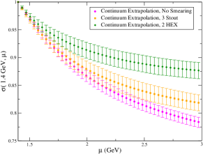
(a) $\sigma_{Z_{m}}(1.4\text{ GeV},\mu)$ Extrapolated

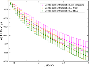
(b) $\sigma_{Z_{q}}(1.4\text{ GeV},\mu)$ Extrapolated

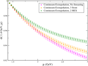
(c) $\sigma_{Z_{T}}(1.4\text{ GeV},\mu)$

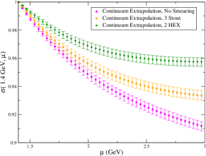
(d) $\sigma_{Z_{BK}}(1.4\text{ GeV},\mu)$

Figure 5: The step scaling functions extrapolated to $a^{2}=0$. (a) $Z_{m}$ (b) $Z_{q}$ (c) $Z_{T}$ (d) $Z_{BK}$

Comparing the perturbation theory with the lattice data only the unsmeared data seems to be asymptotically approaching the perturbative result at high energy, the smeared data overshoots and badly disagrees. The size of the disagreement between the anomalous dimensions does not affect the step scaling plots as much because in this region the absolute value of the anomalous dimension itself is smaller, only when integrated over a sizable energy range does this effect become apparent, for example the last point $\sigma_{Z_{m}}(1.4\text{ GeV},3\text{ GeV})$ is clearly different depending on the smearing prescription. Table 4 gives the values of this step scaling function with the different smearings and a significant (up to 10%) difference is observed for this quantity, which happens to be the worst we have studied. Calculations performed using smeared gauge fields will give final results at high scales significantly different than with unsmeared gauge fields, the difference is larger than the sub percent errors commonly expected for NPR and should be accounted for or avoided by staying at low scales ($\ll a^{-1}$).

	$\gamma_{1}$	$\gamma_{2}$	$\gamma_{3}$
$Z_{m}$	4	66.4763	1030.17
$Z_{q}$	0	6.33333	99.5426
$Z_{T}$	1.33333	23.6932
$Z_{BK}$	2	1.26007

$\alpha_{s}(1\text{GeV})$	$\alpha_{s}(2\text{GeV})$	$\alpha_{s}(3\text{GeV})$
0.480637	0.295752	0.245273

Table 3: Coefficients of the anomalous dimension in the RI/SMOM schemes used in this work. Numerical values of the $\overline{MS}$ coupling are also listed.

	Unsmeared	3 Stout	2 HEX
$\sigma_{Z_{m}}$	0.782(9)	0.817(15)	0.876(15)
$\sigma_{Z_{q}}$	0.9891(12)	0.9869(12)	0.9870(10)
$\sigma_{Z_{T}}$	0.9231(19)	0.9313(20)	0.9448(17)
$\sigma_{Z_{BK}}$	0.9111(32)	0.9332(34)	0.9575(30)

Table 4: The step scaling functions from $1.4$ to $3.0$ GeV, for four different quantities using two types of smearing compared to the unsmeared. For large steps the differences can be large.

\psfrag{Perturbation Theory}{\Huge Continuum}\includegraphics*[angle={0},width=195.12767pt]{gamma_Zm_cl_NE_bmwhex2_3.0_1.0.eps}

(a) $\gamma_{Z_{m}}(\mu)$ Extrapolated

\psfrag{Perturbation Theory}{\Huge Continuum}\includegraphics*[angle={0},width=195.12767pt]{gamma_Zq_cl_NE_bmwhex2_3.0_1.0.eps}

(b) $\gamma_{Z_{q}}(\mu)$ Extrapolated

\psfrag{Perturbation Theory}{\Huge Continuum}\includegraphics*[angle={0},width=195.12767pt]{gamma_ZT_cl_NE_bmwhex2_3.0_1.0.eps}

(c) $\gamma_{Z_{T}}(\mu)$ Extrapolated

\psfrag{Perturbation Theory}{\Huge Continuum}\includegraphics*[angle={0},width=195.12767pt]{gamma_Zbk_cl_NE_bmwhex2_3.0_1.0.eps}

(d) $\gamma_{Z_{BK}}(\mu)$ Extrapolated

Figure 6: The $a^{2}$ extrapolated anomalous dimension of (a)$Z_{m}$, (b) $Z_{q}$, (c) $Z_{m}$ and (d) $Z_{B_{K}}$. With three smearing prescriptions, none, 3 Stout and 2 HEX overlayed.

The plots in Figure 6 show the anomalous dimensions for the quark mass, field, the tensor and $B_{K}$ renormalization. In all cases a similar story is observed. Up to some low scale the continuum limits all agree, as required for a universal continuum limit. However, upon going higher they disagree indicating lattice artefacts beyond $O(a^{2})$. From the anomalous dimension plots the unsmeared data seems to follow the perturbative prediction more closely.

V Conclusions

The principle observation is that an $O(a^{2})$ extrapolation will not restore agreement between smeared and unsmeared data when it includes lattice momenta that are sufficiently high to resolve the smearing radius. Naturally, if a sufficiently fine lattice were used at a fixed physical momentum universality would be restored.

The inverse lattice spacing for the coarse lattice is approximately $1.75\text{ GeV}$ Allton:2008pn which is about the scale at which the difference between the stout and unsmeared cases begins to emerge. The stronger smearing, HEX, begins to disagree sooner although the exact scale at which there is a disagreement depends on the operator. The implication of our data is that the upper end of the Rome Southampton window is being lowered by the smearing. The smearing introduces a new scale into the problem, lower than the original lattice cut-off, and extrapolating at scales above that with a low order $a^{2}$ ansatz will yield incorrect results.

Comparing the anomalous dimensions it seems that the unsmeared data is asymptotically approaching perturbation theory, and is quite close already in the range of momenta we have used. The smeared data agrees with the unsmeared up to a certain scale, as required for a universal continuum limit, but disagrees for larger momenta within the range of our data. The unsmeared data also overshoots the perturbative anomalous dimension, and does not appear to be asymptotically joining the curve. This is almost certainly the result of a pinched Rome-Southampton window introducing lattice artefacts not described by our $O(a^{2})$ extrapolation. Were sufficiently fine lattices used with these physical scales we expect that the smeared data would then approach the unsmeared and asymptotically approach the perturbative curve.

This implies that there is a highest lattice momentum we can use for NPR which depends on the smearing type and is lower for larger smearing radii. Although strictly speaking we do not know that the unsmeared calculation is lattice artefact free at all scales considered, we can use this as a comparison point and look at the scale at which the smeared and unsmeared begin to disagree, this also depends on the operator and the size of the errors so that being quantitative is difficult. At most we can say with confidence that this scale is lower than about 2 GeV in physical units and smaller for 2 HEX than 3 Stout with our combination of $1.7$ and $2.3$ GeV lattice spacings.

Smearing the gauge fields has a significant cost benefit for Wilson and chiral fermions, and is becoming ubiquitous in lattice calculations. However when combined with non-perturbative renormalization there are some pitfalls.

We can illustrate this by considering how large an error would have been introduced by using smeared link step scaling functions in place of thin link for a recent RBC-UKQCD calculation. Step scaling functions, computed on the lattices we have used for this work, have been used by RBC/UKQCD to raise the renormalization scale in previous work, :2012opa . In this paper a coarse lattice spacing was used $a^{-1}=1.37(1)\text{ GeV}$ meaning that for NPR only low scales were safely accessible. However using two finer lattices step scaling functions were produced to raise the renormalization scale up to $3\text{ GeV}$ thereby reducing the perturbative conversion error significantly. The $a^{-1}=1.37(1)\text{ GeV}$ lattice in this paper used a different action than the lattices used to calculate the step scaling functions however universality of the continuum limit was used to argue that combining two separate continuum limits introduced errors of $O(a^{4})$.

The step scaling function for the mass calculated in reference :2012opa was $0.797(8)$, see table XVII in this work, reproduced within errors here in table 4, (we used different configurations and a different fitting procedure compared to :2012opa ). The $\overline{MS}$ quark masses calculated in :2012opa were

$$m_{ud}^{\overline{MS}}(3\text{ GeV})=3.05(10)\text{ MeV}\,\,\,\,m_{s}^{\overline{MS}}(3\text{ GeV})=83.5(2.0)\text{ MeV}.$$ (27)

Using $\frac{\sigma_{Zm}^{\text{stout3}}(1.4,3)}{\sigma_{Zm}^{\text{none}}(1.4,3)}=1.025$ and $\frac{\sigma_{Zm}^{\text{hex2}}(1.4,3)}{\sigma_{Zm}^{\text{none}}(1.4,3)}=1.099$ would change the quark masses significantly more than the indicated error:

$$m_{ud}^{\overline{MS}}(3\text{ GeV},\text{3 Stout})=3.13(10)\text{ MeV}\,\,\,\,m_{s}^{\overline{MS}}(3\text{ GeV},\text{3 Stout})=85.6(2.1)\text{ MeV}$$ (28)

$$m_{ud}^{\overline{MS}}(3\text{ GeV},\text{2 HEX})=3.35(11)\text{ MeV}\,\,\,\,m_{s}^{\overline{MS}}(3\text{ GeV},\text{2 HEX})=91.8(2.2)\text{ MeV}.$$ (29)

Now that calculations of key parameters such as quark masses and $B_{K}$ have become so precise the effect of smearing on NPR can be a dominant systematic error if not properly controlled. Proper control appears to require keeping the lattice momenta $(ap)^{2}\leq 1$ for all vertex functions included in the renormalisation due to the pinched Rome-Southampton window, while we found that unsmeared data can make use of somewhat larger lattice momenta. We also found that the effects of stout smearing (at 2.5%) were much smaller than the effects of HEX smearing (at 10%). Both of these could have been avoided with more conservative lattice momenta, but this would have prevented the successful connection with perturbation theory at 3 GeV.

The observed trends in the reduced anomalous dimension at high energy as well as the flattening of the step scaling functions and the renormalization constants moving closer to one are a strong indication, though not a proof, that smearing reduces the effective lattice cut-off.

We note that the effect of reduced perturbative corrections has been loosely described as showing that smearing gauge fields brings the theory closer to the continuum limit. In this paper we have presented clear evidence based on smeared fermionic vertex functions that such gauge fields possess a second, hidden, coarse lattice spacing associated with the smearing radius, and introduce a narrower Rome-Southampton scaling window. In light of the removal of the UV content of the gauge field, and the results of this paper, we find it is perhaps more accurate to describe smeared gauge fields as closer to the trivial configuration in a momentum region where QCD has real dynamics to describe, particularly if we seek to run, non-perturbatively, into the perturbative regime to connect to perturbation theory.

Renormalizing at lower scales is not a problem in principle for lattice calculations. A problem arises when performing a perturbative conversion to the $\overline{MS}$ scheme. The perturbative expansions do not converge very well at low energy and raising the scale by even $1\text{ GeV}$ can dramatically reduce the perturbative systematic error. However, this is expensive to do by brute force. As such, combining Rome-Southampton renormalization at low scales with some safe, non-perturbative running to high scales before converting may be necessary for high precision calculations of renormalization constants on smeared backgrounds.

If future ensembles are generated using smeared links then step scaling functions Arthur:2010ht may be useful for reducing systematic errors in renormalization calculations by allowing us to always operate within a safe momentum range.

References

- (1) C. Morningstar and M. J. Peardon, Phys. Rev. D 69 (2004) 054501 [hep-lat/0311018].
- (2) S. Capitani, S. Durr and C. Hoelbling, JHEP 0611 (2006) 028 [hep-lat/0607006].
- (3) K. Orginos et al. [MILC Collaboration], Phys. Rev. D 60 (1999) 054503 [hep-lat/9903032].
- (4) C. W. Bernard and T. A. DeGrand, Nucl. Phys. Proc. Suppl. 83 (2000) 845 [hep-lat/9909083].
- (5) A. Hasenfratz, R. Hoffmann and S. Schaefer, JHEP 0705 (2007) 029 [hep-lat/0702028].
- (6) D. J. Antonio et al. [RBC and UKQCD Collaborations], Phys. Rev. D 77 (2008) 014509 [arXiv:0705.2340 [hep-lat]].
- (7) Leinweber, Derek B. et al.[UKQCD collaboration], Phys. Rev. D 58 (1998) 031501 [arxiv:9803015 [hep-lat]].
- (8) G. Martinelli, C. Pittori, C. T. Sachrajda, M. Testa and A. Vladikas, Nucl. Phys. B 445 (1995) 81 [hep-lat/9411010].
- (9) M. Gockeler, R. Horsley, H. Oelrich, H. Perlt, D. Petters, P. E. L. Rakow, A. Schafer and G. Schierholz et al., Nucl. Phys. B 544 (1999) 699 [hep-lat/9807044].
- (10) Y. Aoki, P. A. Boyle, N. H. Christ, C. Dawson, M. A. Donnellan, T. Izubuchi, A. Juttner and S. Li et al., Phys. Rev. D 78 (2008) 054510 [arXiv:0712.1061 [hep-lat]].
- (11) R. Arthur et al. [RBC and UKQCD Collaborations], Phys. Rev. D 83 (2011) 114511 [arXiv:1006.0422 [hep-lat]].
- (12) , et al. [RBC and UKQCD Collaborations], arXiv:1208.4412 [hep-lat].
- (13) Y. Aoki, R. Arthur, T. Blum, P. A. Boyle, D. Brommel, N. H. Christ, C. Dawson and T. Izubuchi et al., Phys. Rev. D 84 (2011) 014503 [arXiv:1012.4178 [hep-lat]].
- (14) S. Durr, Z. Fodor, C. Hoelbling, S. D. Katz, S. Krieg, T. Kurth, L. Lellouch and T. Lippert et al., JHEP 1108 (2011) 148 [arXiv:1011.2711 [hep-lat]].
- (15) A. Hasenfratz and F. Knechtli, Phys. Rev. D 64 (2001) 034504 [hep-lat/0103029].
- (16) Y. Shamir, B. Svetitsky and E. Yurkovsky, Phys. Rev. D 83 (2011) 097502 [arXiv:1012.2819 [hep-lat]].
- (17) C. Aubin, J. Laiho and R. S. Van de Water, Phys. Rev. D 81 (2010) 014507 [arXiv:0905.3947 [hep-lat]].
- (18) S. Durr, Z. Fodor, C. Hoelbling, S. D. Katz, S. Krieg, T. Kurth, L. Lellouch and T. Lippert et al., Phys. Lett. B 705 (2011) 477 [arXiv:1106.3230 [hep-lat]].
- (19) T. Kurth et al. [Budapest-Marseille-Wuppertal Collaboration], PoS LATTICE 2010 (2010) 232 [arXiv:1011.1780 [hep-lat]].
- (20) C. Allton et al. [RBC-UKQCD Collaboration], Phys. Rev. D 78 (2008) 114509 [arXiv:0804.0473 [hep-lat]].
- (21) Y. Aoki et al. [RBC and UKQCD Collaborations], Phys. Rev. D 83 (2011) 074508 [arXiv:1011.0892 [hep-lat]].
- (22) C. Sturm, Y. Aoki, N. H. Christ, T. Izubuchi, C. T. C. Sachrajda and A. Soni, Phys. Rev. D 80 (2009) 014501 [arXiv:0901.2599 [hep-ph]].
- (23) M. Luscher, R. Sommer, P. Weisz and U. Wolff, Nucl. Phys. B 413 (1994) 481 [hep-lat/9309005].
- (24) L. G. Almeida and C. Sturm, Phys. Rev. D 82 (2010) 054017 [arXiv:1004.4613 [hep-ph]].