Exciton dynamics in emergent Rydberg lattices

Abstract

The dynamics of excitons in a one-dimensional ensemble with partial spatial order are studied. During optical excitation, cold Rydberg atoms spontaneously organize into regular spatial arrangements due to their mutual interactions. This emergent lattice is used as the starting point to study resonant energy transfer triggered by driving a $nS$ to $n^{\prime}P$ transition using a microwave field. The dynamics are probed by detecting the survival probability of atoms in the $nS$ Rydberg state. Experimental data qualitatively agree with our theoretical predictions including the mapping onto XXZ spin model in the strong-driving limit. Our results suggest that emergent Rydberg lattices provide an ideal platform to study coherent energy transfer in structured media without the need for externally imposed potentials.

I Introduction

The investigation of far-from-equilibrium phenomena overarches the fields of physics, chemistry and biology. Systems out of equilibrium feature fascinating phenomena such as the formation of complex ordered structures in spite of a rather simple underlying microscopic description Cross and Hohenberg (1993). Moreover, dynamical phenomena such as resonant energy transfer are of central practical importance as they underlie many fundamental physical processes in molecular aggregates Scholes (2003), photosynthesis Engel et al. (2007) and novel materials such as organic solar cells Scholes and Rumbles (2006).

Gases of cold atoms have been established in the past years as a platform which permits the detailed investigation of systems in and out of equilibrium Mottl et al. (2012); Gring et al. (2012); Trotzky et al. (2012). Recently atoms excited to high-lying Rydberg states have become a major focus due to their strong interactions over large distances (several micrometers) and short time scales (nanoseconds) allowing to address fundamental questions in many-body physics. On the one hand the strong interactions give rise to the phenomenon of dipole blockade Lukin et al. (2001) which prevents simultaneous photo-excitation of nearby atoms. On the other hand the large dipole moments associated with electronic transitions among Rydberg states lead to fast resonant energy transfer over long distances.

Dipole blockade has been widely exploited for applications in quantum information processing Saffman et al. (2010) and quantum optics Pritchard et al. (2010); Sevinçli et al. (2011); Petrosyan et al. (2011); Dudin and Kuzmich (2012); Peyronel et al. (2012); Gorshkov et al. (2013). In the many-body context, spatial correlations of laser-excited atoms were recently investigated theoretically in one-dimensional finite-size samples Ates and Lesanovsky (2012); Breyel et al. (2012); Gärttner et al. (2012); Höning et al. (2013). It was found that at high atomic density the distribution of the Rydberg atoms can become highly structured leading in the extreme case to the spontaneous formation of small ordered patches consisting of a few Rydberg atoms. From the experimental side much effort has been invested to probe these spatial correlations Schwarzkopf et al. (2011); Dudin et al. (2012); Schauß et al. (2012). In parallel, resonant energy transfer has been the focus of pioneering experiments on cold (frozen) Rydberg gases Mourachko et al. (1998); Anderson et al. (1998). Spectral broadening of Rydberg lines could be attributed to coherent electronic energy transfer between Rydberg atoms. These findings have ushered further experimental Li et al. (2005); van Ditzhuijzen et al. (2008); Nipper et al. (2012); Maxwell et al. (2013) as well as theoretical Frasier et al. (1999); Robicheaux et al. (2004); Mülken et al. (2007); Müller et al. (2008); Wüster et al. (2010, 2011); Scholak et al. (2011); Kiffner et al. (2012); Bariani et al. (2012) efforts to analyze excitonic transfer processes and their consequences in cold Rydberg systems.

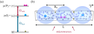
Figure 1: (Color online) (a) Rydberg levels and excitation scheme. In step 1 atoms are optically excited from their electronic ground state $|g\rangle$ to a highly-excited state $|nS\rangle$ with effective Rabi frequency $\Omega_{\text{Ryd}}$. Subsequently, in step 2, a microwave field is applied that couples the $|nS\rangle$ state to a nearby $|n^{\prime}P\rangle$ level with Rabi frequency $\Omega_{\text{MW}}$. These states are identified as internal states of a fictitious spin-1/2 particle. (b) Quasi one-dimensional geometry of the system. The large van der Waals potential between the $|nS\rangle$ Rydberg atoms (blue spheres) induces an exclusion volume around each excited atom characterized by the blockade radius $R_{\rm b}$ larger than the transverse size of the sample. This leads to a highly structured density distribution of the Rydberg atoms after the laser excitation step. The transition dipole-dipole interaction induces a coherent spatial transfer of $(n^{\prime}P)$-excitations.

In this work we build on these developments and present a study of the out-of-equilibrium behavior of Rydberg gases that directly links to the above-mentioned themes of order formation and excitation transfer. We explore the electronic dynamics of a (quasi) one-dimensional Rydberg gas within a two-step protocol, see Fig. 1. In step 1 high-lying Rydberg $nS$-states are optically excited leading to the spontaneous emergence of a lattice of Rydberg atoms immersed in the atomic gas of ground state atoms. In the subsequent step 2 we trigger coherent excitation transfer between Rydberg atoms by the excitation of nearby Rydberg $n^{\prime}P$-states via a microwave field. We theoretically investigate the resulting non-equilibrium exciton dynamics through the analysis of the survival probability of atoms in the Rydberg $nS$-state. We show that the survival probability has a characteristic dependence on the spatial arrangement as well as on the number of Rydberg atoms and derive an effective Hamiltonian in the limit of strong microwave driving. We compare our theoretical predictions with an experiment in which the survival probability is measured through an optical read-out protocol and find qualitative agreement. Our work shows the versatility of homogeneous gases of Rydberg atoms for the study of non-equilibrium processes such as coherent transport phenomena.

The paper is organized as follows: In section II we theoretically describe and investigate the spontaneous formation of lattices of Rydberg atoms upon photo-excitation from a one-dimensional finite-size atomic gas. Subsequently, we discuss the electronic dynamics when the excited atoms are coupled to a nearby Rydberg state by a microwave (section III). In particular, we illuminate on the connection between the electronic dynamics with the underlying ordering of the Rydberg atoms. Finally, in section IV we present experimental data that are obtained using a similar protocol as the one discussed in this work and find qualitative agreement between experiment and theory. Unless stated otherwise we will work in units where $\hbar=1$.

II Emergent lattice

First we introduce the framework within which we describe exciton dynamics in an emergent lattice (cf. Fig. 1). We consider a one-dimensional atomic gas of length $L$ with homogeneous density $\rho=N/L$, where $N$ denotes the total number of atoms and we set our quantization axis ($z$) along the long axis of the gas. In order to describe the electronic dynamics, we use a simplified level scheme in which each atom is modeled by using three levels: the electronic ground state $|g\rangle$ and two dipole-coupled, highly excited states $|nS\rangle$ and $|n^{\prime}P\rangle$ with principal quantum numbers $n$ and $n^{\prime}$ and angular momentum $l=0$ ($S$) and $l=1$ ($P$), respectively. The actual states used in the experiment will be discussed later.

In the first step of our protocol, atoms are optically excited from $|g\rangle$ to $|nS\rangle$. The dynamics in this step are dominated by the strong van der Waals interaction between Rydberg atoms. Such interactions shift many-body states containing pairs of Rydberg atoms closer than a critical distance out of resonance. Consequently each excited atom is surrounded by a blockade volume of radius $R_{b}$, within which no further Rydberg excitations are found. For our finite, one-dimensional, homogeneous system this dipole blockade mechanism restricts the maximum number of Rydberg excitations to $\nu_{\text{max}}=\lfloor L/R_{b}\rfloor+1$, where $\lfloor x\rfloor$ denotes the closest integer smaller than $x$. We have assumed a sharply defined blockade volume which is justified in case of a one-dimensional system and rapidly decaying van der Waals interaction Ates and Lesanovsky (2012); Petrosyan et al. (2013). The quantum state after the laser excitation (i.e., the initial state of the microwave driving) can be formally written as

$$|\Psi_{0}\rangle=\sum_{\nu=0}^{\nu_{\text{max}}}\sum_{1\leq\alpha_{1}<\dots<\alpha_{\nu}\leq N}g^{(\nu)}_{\alpha_{1}\dots\alpha_{\nu}}\left(\prod_{j=1}^{\nu}e^{-ikz_{\alpha_{j}}}S^{+}_{\alpha_{j}}\right)|0\rangle.$$ (1)

Here, $|0\rangle=\bigotimes_{i}|g\rangle_{i}$ is the Rydberg vacuum, $S^{+}_{i}=|nS\rangle\langle g|_{i}$ is the operator that creates a Rydberg atom at position $z_{i}$ and $k$ is the total momentum imposed by the excitation laser(s), where we assume $\hat{k}\parallel\hat{z}$. In general, this state is highly correlated and the coefficients $g^{(\nu)}_{\alpha_{1}\dots\alpha_{\nu}}\equiv g^{(\nu)}(z_{\alpha_{1}},\dots,z_{\alpha_{\nu}})$ depend on the positions of all excited atoms and on time (the time label was suppressed to shorten the notation). These correlations, which dynamically build up during the laser-excitation, render a full quantum calculation of $|\Psi_{0}\rangle$ a formidable task.

However, as recently shown numerically Lesanovsky et al. (2010) and analytically Ates et al. (2012); Ji et al. (2013), for sufficiently large times the strong interactions between Rydberg atoms result in an equilibration. In this saturated regime the moduli of the coefficients $g^{(\nu)}$ of configurations compatible with the Rydberg blockade become equal and constant in time Ates and Lesanovsky (2012). Therefore, observables that depend only on the $|g^{(\nu)}|^{2}\!\!$, such as the Rydberg density and density-density correlations, attain a stationary value. To calculate such ’classical observables’ we use a Monte Carlo method that allows us to sample arrangements of Rydberg atoms compatible with the excitation blockade. The details of the algorithm are given in Appendix A.

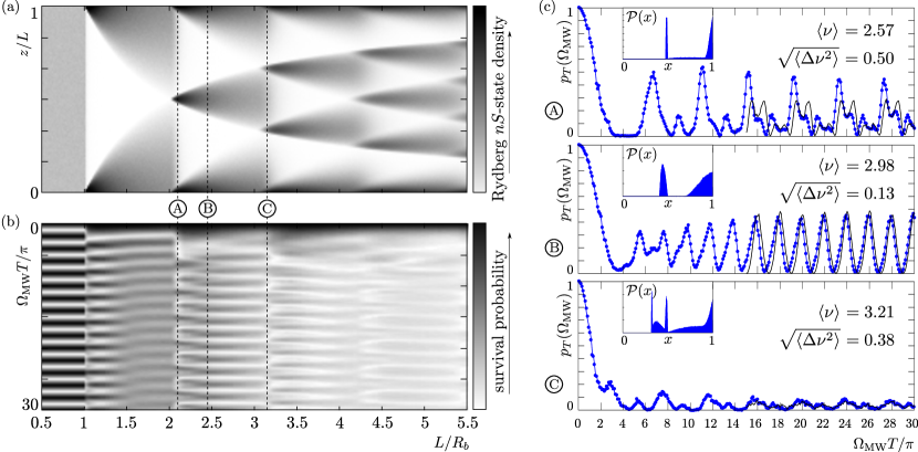
Figure 2: (Color online) (a) Numerically calculated density distribution of Rydberg atoms after laser excitation as a function of the system length $L$ measured in units of the blockade radius $R_{b}$. (b) Survival probability $p_{T}(\Omega_{\text{MW}})$ as a function of $L/R_{b}$ and microwave Rabi frequency $\Omega_{\text{MW}}$. The colormaps in panels (a) and (b) range from 0 (white) to 1 (black). (c) Cuts through the density plot shown in (b) for three different system sizes indicated by the encircled capital letters. The corresponding mean, $\langle\nu\rangle$, and variance, $\sqrt{\left(\Delta\nu^{2}\right)}$, of the Rydberg atom number distribution are indicated in the panels. The blue symbols show numerical results from the Hamiltonian given in eq. (2) and the solid black lines are obtained using the effective Hamiltonian (5) valid for large $\Omega_{\text{MW}}$. The statistical distribution of the dipole-dipole interaction energy between atom pairs is shown in the insets. For better visibility we show the distributions as a function of $x=(\mathcal{V}R^{3}_{b}/\mu^{2})^{1/3}$, i.e. the third root of the interaction strength at the blockade distance $R_{b}$. The data shown in panels (b) and (c) were obtained by averaging over 400 initial configurations generated by Monte Carlo sampling. In (b) and (c) the dipole-dipole interaction strength, $V(R_{b})$, for an atom pair separated by $R_{b}$ is $V(R_{b})T=15$.

Fig. 2(a) shows the numerically calculated stationary Rydberg density distributions as a function of the system length $L$ for a gas consisting of $N=10^{4}$ atoms at fixed blockade radius and open boundary conditions. For $L>R_{b}$ the plot shows a highly structured density distribution with pronounced peaks at the boundaries of the gas. Whenever the system size slightly exceeds an integer multiple of the blockade radius the density distribution closely resembles a lattice of Rydberg atoms, i.e., the excited atoms are arranged in the densest packing allowed by the excitation blockade. Similar structures have also been reported in Gärttner et al. (2012); Höning et al. (2013); Petrosyan et al. (2013). We emphasize however that the emergence of such seemingly ordered structures is a finite-size effect, as for one-dimensional systems with finite-range interactions spatial correlations decay exponentially with increasing distance in the thermodynamic limit Ates and Lesanovsky (2012).

III Excitonic dynamics

Once the Rydberg lattice is created we trigger the excitonic dynamics by irradiating the ensemble with a microwave field (linearly polarized along the $z$-axis and with Rabi frequency $\Omega_{\text{MW}}$) that is resonant with the $|nS\rangle$-$|n^{\prime}P\rangle$ transition as shown in Fig. 1(a). The corresponding transition dipole moment, $\mu$, can reach thousands of atomic units (scaling as $n^{2}$ for $n=n^{\prime}$). This results in a strong microwave coupling but also induces a significant resonant dipole-dipole interaction enabling excitations to be exchanged coherently between atoms, i.e., two distant Rydberg atoms swap their electronic state according to $|nS\rangle_{i}|n^{\prime}P\rangle_{j}\leftrightarrow|n^{\prime}P\rangle_{i}|nS\rangle_{j}$. For the particular geometry of our system this resonant dipole-dipole interaction does not couple different magnetic sub-levels and the electronic structure of each Rydberg atom reduces to that of an effective spin 1/2 particle where we identify $|nS\rangle\equiv\left|\downarrow\right>$ and $|n^{\prime}P\rangle\equiv\left|\uparrow\right>$. In atomic units the interaction strength is given by $V_{ij}=(-2/3)\mu^{2}/|z_{i}-z_{j}|^{3}$, where $z_{i}$ denotes the position of the $i$-th Rydberg atom Robicheaux et al. (2004). The Hamiltonian describing the resulting dynamics is given by

$$H=\frac{\Omega_{\text{MW}}}{2}\sum_{i}\sigma_{i}^{x}+\sum_{ij,(i\neq j)}V_{ij}\left(\sigma_{i}^{+}\sigma_{j}^{-}+\sigma_{i}^{-}\sigma_{j}^{+}\right)$$ (2)

with $\sigma^{\pm}=(\sigma^{x}\pm{\rm i}\sigma^{y})/2$ and $\sigma^{x,y,z}$ denoting the usual Pauli spin matrices.

In order to study the excitonic dynamics we analyze the survival probability, $p_{T}(\Omega_{\text{MW}})\equiv|\langle\Psi_{0}|e^{-{\rm i}HT}|\Psi_{0}\rangle|^{2}$, of the state $|\Psi_{0}\rangle$. The motivation behind choosing this quantity stems from the fact that $p_{T}(\Omega_{\text{MW}})$ is accessible experimentally, as has been shown recently Maxwell et al. (2013), and that its rich dynamical behavior reveals interesting insights into the physics of the driven exciton system. Following Ref. Maxwell et al. (2013) we numerically determine $p_{T}(\Omega_{\text{MW}})$ for varying strength of the microwave coupling and in addition as a function of the system length for fixed time $T$ and blockade radius $R_{\rm b}$. The results are summarized in Fig. 2(b), where the dipole-dipole interaction strength is chosen such that for two atoms separated by the blockade radius $V(R_{b})T=15.$ Additionally, we present cuts through these data for three selected values of the system length in Fig. 2(c). The survival probability exhibits a rich structure as $L$ and $\Omega_{\text{MW}}$ are varied which, in particular, is clearly correlated to the distribution of Rydberg atoms shown in panel (a). This is most apparent when the system length is close to an integer multiple of the blockade radius, i.e., when an additional Rydberg atom can “fit” into the system. Here, the change in the Rydberg density distribution becomes strikingly visible through a phase jump in the survival probability pattern.

Beyond this global feature, each cut of $p_{T}(\Omega_{\text{MW}})$, taken at a fixed system length $L$, exhibits three distinct regimes as a function of the microwave Rabi frequency [cf. panels of Fig. 2(c)]. For very small $\Omega_{\text{MW}}$ the dynamics is dominated by excitonic energy transfer induced by the dipole-dipole interaction. The system can then be regarded as a number of exciton bands that are weakly coupled by the microwave field. Here, $p_{T}(\Omega_{\text{MW}})$ decreases monotonically with increasing $\Omega_{\text{MW}}$. When the microwave Rabi frequency becomes comparable to the mean dipole-dipole energy, $\langle\mathcal{V}\rangle$, the survival probability exhibits a rather intricate pattern. Here, as well as in the previous regime the exact details of $p_{T}(\Omega_{\text{MW}})$ are very sensitive to the particular distribution of the Rydberg atoms [cf. Fig. 2 (a) and (b)]. This sensitivity is caused by the distance-dependence of the dipole-dipole interaction, which essentially probes the pair distribution function $\mathcal{R}^{(2)}(z,z^{\prime})$ of the Rydberg gas. To see this one can use the formal expression (1) for $|\Psi_{0}\rangle$ to express the survival probability. The resulting expression depends on the distributions $\rho^{(\nu)}(z_{1},\dots,z_{\nu})=|g^{(\nu)}(z_{1},\dots,z_{\nu})|^{2}$ in each particle number subspace, which together determine the pair distribution function through

$$\mathcal{R}^{(2)}(z,z^{\prime})=\sum_{\nu=2}^{\nu_{\text{max}}}\int\text{d}z_{3}\cdots\text{d}z_{\nu}\rho^{(\nu)}(z,z^{\prime},z_{3},\dots,z_{\nu}).$$ (3)

Since the interaction potential has a strong nonlinear dependence on the inter-particle distance even small differences in $\mathcal{R}^{(2)}(z,z^{\prime})$ lead to a significantly modified statistical distribution

$$\mathcal{P}(\mathcal{V})=\int\text{d}z\text{d}z^{\prime}\delta\left(\mathcal{V}-\mu^{2}/|z-z^{\prime}|^{3}\right)\mathcal{R}^{(2)}(z,z^{\prime})$$ (4)

of the dipole-dipole interaction energy $\mathcal{V}$ as shown in the insets of the panels in Fig. 2(c).

Finally, for $\Omega_{\text{MW}}\gg\langle\mathcal{V}\rangle$ the survival probability shows regular oscillations. Most interestingly, as a general trend the amplitude of these oscillations decreases with increasing number of Rydberg atoms in the gas [cf. rightmost part of Fig. 2(b)]. This effect seems counterintuitive as for $\Omega_{\text{MW}}/\langle\mathcal{V}\rangle\gg 1$ one might expect to enter a non-interacting regime in which the microwave drives coherent oscillations between the single atom states $|nS\rangle$ and $|n^{\prime}P\rangle$. This would always lead to oscillation of $p_{T}(\Omega_{\text{MW}})$ with full contrast. However this is a misconception as even for $\Omega_{\text{MW}}/\langle\mathcal{V}\rangle\gg 1$ interactions still play a significant role. This can be understood by deriving the effective Hamiltonian in the limit $V_{ij}\ll\Omega_{\mathrm{MW}}$, starting from eq. (2). To this end, we rotate the spin basis via a unitary transformation $U=\bigotimes_{j}U_{j}$ with $U_{j}=\exp({\rm i}\pi\sigma^{y}_{j}/4)$, which diagonalizes the single-body part of $H$. In the transformed Hamiltonian $UHU^{\dagger}$ we neglect non-resonant terms of the form $\sigma^{+}_{i}\sigma^{+}_{j}$ and $\sigma^{-}_{i}\sigma^{-}_{j}$ that correspond to the simultaneous (de-)excitation of a spin pair. Within this approximation we find that the effective Hamiltonian is that of the spin-$1/2$ XXZ-model,

$$H_{\text{eff}}=\frac{\Omega_{\text{MW}}}{2}\sum_{i}\sigma_{i}^{z}+\sum_{ij,(i\neq j)}\frac{V_{ij}}{4}\left(\sigma_{i}^{x}\sigma_{j}^{x}+\sigma_{i}^{y}\sigma_{j}^{y}+2\sigma_{i}^{z}\sigma_{j}^{z}\right).$$ (5)

This Hamiltonian consists of two commuting parts and thus the microwave driving and the residual dipole-dipole interaction can be treated independently. This shows that no matter how strong $\Omega_{\text{MW}}$ there will always be a nontrivial excitonic dynamics. To illustrate this further let us assume that we are in a regime where the number of Rydberg atoms $\nu_{\text{Ryd}}$ is integer and hence not fluctuating, as e.g. shown in the middle panel of Fig. 2(c). The survival amplitude can now be expressed in terms of a Fourier series, $\langle\Psi_{0}|e^{-iH_{\text{eff}}T}|\Psi_{0}\rangle=B(T)+2\sum_{m=0}^{M}A_{m}(T)\cos(\epsilon_{m}T)$, with $\epsilon_{m}=\Omega_{\text{MW}}(m-\nu_{\text{Ryd}}/2)$ and coefficients $A_{m}(T)$ and $B(T)$ which exclusively depend on the phases $V_{ij}T$ but not on $\Omega_{\text{MW}}$. If $\nu_{\text{Ryd}}$ is odd the summation runs to $M=(\nu_{\text{Ryd}}-1)/2$ otherwise to $M=\nu_{\text{Ryd}}/2-1$. In case of odd $\nu_{\text{Ryd}}$ the symmetry of the Hamiltonian (5) with respect to a global spin flip operation imposes $B(T)=0$. Hence, in this case the survival probability is exactly zero when $\Omega_{\text{MW}}T/\pi$ is an odd integer, which is clearly visible in the middle panel of Fig. 2(c). Note, that in general only if $V_{ij}=0$ the Fourier series can be summed analytically and one consequently obtains the familiar expression for Rabi oscillations of non-interacting particles $|\langle\Psi_{0}|e^{-iH_{\text{eff}}T}|\Psi_{0}\rangle|^{2}=\cos^{2\nu_{\text{Ryd}}}(\Omega_{\text{MW}}T)$.

IV Experiment

We will now conclude with a qualitative comparison of our theoretical results with experimental data. Full details of the experiment can be found in reference Maxwell et al. (2013). In brief, laser-cooled ${}^{87}\mathrm{Rb}$ atoms are loaded into an optical dipole trap forming an elongated cloud with $w_{z}\approx 20~{}\mu$m and $w_{\rm{r}}\approx 0.8~{}\mu$m, where $w$ is the standard deviation of the density distribution. Rydberg $60S_{1/2}$-states are excited with a two-photon transition via the intermediate $5P_{3/2}$-state (see Fig. 3). For the experimental parameters the blockade radius is $R_{\rm b}\approx 7~{}\mu\text{m}\gg w_{\rm{r}}$ and hence the setup is quasi-one-dimensional as illustrated in Fig. 1(b). The optical excitation fields are applied for a sufficiently long time that saturation is reached (see right inset of Fig. 3 and corresponding caption). This corresponds to step 1, i.e. the preparation of the emergent lattice. Subsequently, the lasers are switched off and a microwave field (step 2, driving the exciton dynamics), couples the states $\left|60S_{1/2}\right>$ and $|59P_{3/2}\rangle$, for a time $T=150$ ns. After step 2 the Rydberg excitations in state $60S_{1/2}$ are converted into photons by switching on the control field, see Maxwell et al. (2013). The resulting photon-retrieval probability, $\mathrm{P}$, is proportional to the survival probability $p_{T}(\Omega_{\text{MW}})$ Maxwell et al. (2013) and plotted in Fig. 3 as a function of the microwave Rabi frequency, $\Omega_{\text{MW}}$.

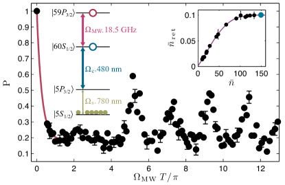
Figure 3: (Color online). Experimentally measured photon retrieval probability, $\mathrm{P}$, as a function of the microwave Rabi frequency $\Omega_{\text{MW}}$. The duration of the microwave pulse, $T=150$ ns, is fixed. Inset: (Left) Excitation scheme used in the experiment. The Rydberg $60S_{1/2}$-state is reached by a two-photon transition via the $5P_{3/2}$-state. A microwave field couples the $60S_{1/2}$-state to the $59P_{3/2}$-state. (Right) As the number of photons $\bar{n}$ in the signal field (proportional to the Rabi frequency $\Omega_{\mathrm{s}}$ and pulse duration) is increased, the number of retrieved photons $\bar{n}_{\mathrm{ret}}$ saturates in the absence of microwave driving. The data shown in the main plot is obtained well within this saturated regime (blue point). The lines are a guide to the eye.

Remarkably, this data shows qualitatively the same features as the discussed theoretical model, i.e., a quick decay of the survival probability, followed by increasingly regular oscillations. In fact the shape of the curve follows quite closely the behavior depicted in the middle panel of Fig. 2c. This is despite the fact that details of the experiment, e.g. the excitation scheme and the Gaussian atomic density distribution, differ from the underlying theoretical model.

V Conclusions

In this work we have studied the dynamics of a two-step protocol that consists (i) of photo-exciting Rydberg atoms from an one-dimensional ultracold gas and (ii) subsequently inducing excitonic energy transfer in the highly correlated Rydberg gas using a microwave field. In the regime of weak microwave driving we have shown that the exciton dynamics strongly depends on the spatial arrangement of the Rydberg atoms. This connection opens up the possibility of using the second step of our protocol as a diagnostic tool for mapping out the spatial structure of highly correlated Rydberg gases. In the opposite limit of strong microwave driving we have shown that the dynamics of the system is governed by the Hamiltonian of the XXZ model. This highlights the applicability of simple models to describe and understand complex experiments to investigate non-equilibrium exciton dynamics in ultracold Rydberg systems.

Appendix A Configuration-selection algorithm

The Monte-Carlo algorithm that we have used to obtain our numerical data relies on the generation of excitation configurations (that are compatible with the Rydberg blockade) ’on the fly’. It is composed of a preparation stage and an actual drawing stage.

Preparation stage – In the first stage we prepare two tables ($c(j,k)$ and $n(j)$) that we will use to quickly generate random configurations in the second stage of our algorithm. To this end we label the $N$ atoms from left to right with an index $j$ and define $c(j,k)$ to be the number of allowed configurations (compatible with the blockade) with $k\geq 0$ excitations in the index range $[j,N]$ and zero excitations in the range $[1,j-1]$. Furthermore, we define $n(j)>j$ as the index of the first atom to the right of a Rydberg atom at position $j$ that lies outside the blockade radius. With these definitions the following recursive relation holds for $k>1$,

$$c(j,k)={\textstyle\sum_{q=j}^{N}}\,\,c(n(q),k-1),$$ (6)

with initial conditions $c(j,0)=1$ and $c(j,1)=N-j+1$. This permits the calculation of the total number $\mathcal{N}$ of allowed configurations as well as the fraction $p_{k}$ of configurations with exactly $k$ excitations, according to the formulae $\mathcal{N}=\sum_{k\geq 0}c(1,k)$ and $p_{k}=c(1,k)/\mathcal{N}$.

In order to illustrate the procedure, let us take $N=7$ atoms spaced as in the following diagram (where the distance between two vertical bars is one blockade radius)

                                                                              $\bullet$        $\bullet$         $\bullet$       $\bullet$               $\bullet$       $\bullet$        $\bullet$
          1        2         3       4               5       6        7

The corresponding values of $n(j)$ and $c(j,k)$ are then

$j$	$n(j)$
1	3
2	4
3	5
4	5
5	7
6
7

$j\backslash^{\!\displaystyle k}$	0	1	2	3	4
1	1	7	16	13	3
2	1	6	11	6	1
3	1	5	7	2
4	1	4	4	1
5	1	3	1
6	1	2
7	1	1
$p_{k}$	$\tfrac{1}{40}$	$\tfrac{7}{40}$	$\tfrac{16}{40}$	$\tfrac{13}{40}$	$\tfrac{3}{40}$

Therefore, $\nu_{\text{max}}=4$, $\mathcal{N}=\sum_{k}c(1,k)=40$.

Note that the $\mathcal{N}$ actual configurations are never explicitly generated (as the resources in time and memory would scale exponentially with $N$), but for sake of clarity the $40$ possible ones are:

#	#	actual configurations
excit	config	(excited atoms shown in parentheses)
0	1	();
1	7	(1), (2), (3), (4), (5), (6), (7);
2	16	(13), (14), (15), (16), (17), (24), (25), (26),
		(27), (35), (36), (37), (45), (46), (47), (57);
3	13	(135),(136),(137),(145),(146),(147),(157),
		(245),(246),(247),(257),(357),(457);
4	3	(1357), (1457), (2457).

Drawing stage – Once the $c(j,k)$ table is ready, we can use it to randomly sample the space of allowed configurations. To this end we draw a random integer $m$ in the range $[1,\mathcal{N}]$. In order to uniquely ascribe a specific configuration to $m$ we use the convention that configurations are first ordered according to the number $\nu$ of excitations and then lexicographically over the indexes of excited atoms. The search is implemented first scanning the entries $c(1,k)$ till $\nu$ is determined, then using the entries $c(j,\nu)$ to find the actual excitation positions. In C pseudo-code the algorithm reads:

k=0; j=1;
while (m>c(1,k)) {m-=c(1,k); ++k;} // step 1
while (k>1) { q=j; // step 2
  while (m>c(n(q),k-1)) {m-=c(n(q),k-1); ++q;}
  mark_as_excited(q); j=n(q); --k; }
if (k>0) mark_as_excited(j+m-1);

Let us see how this works in the example for $m=35$:

• $m>c(1,0)=1\Rightarrow$ not the configuration with zero excitations, then update $m\rightarrow m-c(1,0)=34$;

• $m>c(1,1)=7\Rightarrow$ not a configuration with one excitation, then update $m\rightarrow m-c(1,1)=27$;

• $m>c(1,2)=16\Rightarrow$ not a configuration with two excitations, then update $m\rightarrow m-c(1,2)=11$;

• $m\leq c(1,3)=13\Rightarrow$ the selected configuration has $\nu=3$ excitations; let us look for their indexes;

• $m>c(n(1),\nu-1)=7\Rightarrow$ the first index is larger than 1, then update $m\rightarrow m-c(n(1),\nu-1)=4$;

• $m\leq c(n(2),\nu-1)=4\Rightarrow$ the first index is $j_{1}=2$; let us look for the second one (from $n(j_{1})=4$ on);

• $m>c(n(4),\nu-2)=3\Rightarrow$ the second index is larger than 4, then update $m\rightarrow m-c(n(4),\nu-2)=1$;

• $m\leq c(n(5),\nu-2)=1\Rightarrow$ the second index is $j_{2}=5$; let us look for the last one;

• the last index is just $n(j_{2})+m-1=7+1-1=7$, then the selected configuration is (257).

Using this procedure repeatedly, we can generate a random sequence $\mathcal{S}=\{m_{1},m_{2},\dots,m_{K}\}$ of $K$ allowed configuration, where each configuration is drawn with equal probability $1/\mathcal{N}$. Classical observables like the local Rydberg density $\langle n_{i}\rangle$ or density-density correlations $\langle n_{i}n_{j}\rangle$ can then be determined as

$$\langle n_{i}\rangle \approx \frac{1}{K}\sum_{\mathcal{S}}\left(n_{i}\right)_{\mathcal{S}}$$ (7)

$$\langle n_{i}n_{j}\rangle \approx \frac{1}{K}\sum_{\mathcal{S}}\left(n_{i}n_{j}\right)_{\mathcal{S}}.$$ (8)

References

- Cross and Hohenberg (1993) M. C. Cross and P. C. Hohenberg, Rev. Mod. Phys. 65, 851 (1993).
- Scholes (2003) G. D. Scholes, Annual Review of Physical Chemistry 54, 57 (2003).
- Engel et al. (2007) G. S. Engel, T. R. Calhoun, E. L. Read, T.-K. Ahn, T. Mancal, Y.-C. Cheng, R. E. Blankenship, and G. R. Fleming, Nature 446, 782 (2007).
- Scholes and Rumbles (2006) G. D. Scholes and G. Rumbles, Nat Mater 5, 683 (2006).
- Mottl et al. (2012) R. Mottl, F. Brennecke, K. Baumann, R. Landig, T. Donner, and T. Esslinger, Science 336, 1570 (2012).
- Gring et al. (2012) M. Gring, M. Kuhnert, T. Langen, T. Kitagawa, B. Rauer, M. Schreitl, I. Mazets, D. A. Smith, E. Demler, and J. Schmiedmayer, Science 337, 1318 (2012).
- Trotzky et al. (2012) S. Trotzky, Y.-A. Chen, A. Flesch, I. P. McCulloch, U. Schollwock, J. Eisert, and I. Bloch, Nat Phys 8, 325 (2012).
- Lukin et al. (2001) M. D. Lukin, M. Fleischhauer, R. Côté, L. M. Duan, D. Jaksch, J. I. Cirac, and P. Zoller, Phys. Rev. Lett. 87, 037901 (2001).
- Saffman et al. (2010) M. Saffman, T. G. Walker, and K. Mølmer, Rev. Mod. Phys. 82, 2313 (2010).
- Pritchard et al. (2010) J. D. Pritchard, D. Maxwell, A. Gauguet, K. J. Weatherill, M. P. A. Jones, and C. S. Adams, Phys. Rev. Lett. 105, 193603 (2010).
- Sevinçli et al. (2011) S. Sevinçli, N. Henkel, C. Ates, and T. Pohl, Phys. Rev. Lett. 107, 153001 (2011).
- Petrosyan et al. (2011) D. Petrosyan, J. Otterbach, and M. Fleischhauer, Phys. Rev. Lett. 107, 213601 (2011).
- Dudin and Kuzmich (2012) Y. O. Dudin and A. Kuzmich, Science 336, 887 (2012).
- Peyronel et al. (2012) T. Peyronel, O. Firstenberg, Q.-Y. Liang, S. Hofferberth, A. V. Gorshkov, T. Pohl, M. D. Lukin, and V. Vuletic, Nature 488, 57 (2012).
- Gorshkov et al. (2013) A. V. Gorshkov, R. Nath, and T. Pohl, Phys. Rev. Lett. 110, 153601 (2013).
- Ates and Lesanovsky (2012) C. Ates and I. Lesanovsky, Phys. Rev. A 86, 013408 (2012).
- Breyel et al. (2012) D. Breyel, T. L. Schmidt, and A. Komnik, Phys. Rev. A 86, 023405 (2012).
- Gärttner et al. (2012) M. Gärttner, K. P. Heeg, T. Gasenzer, and J. Evers, Phys. Rev. A 86, 033422 (2012).
- Höning et al. (2013) M. Höning, D. Muth, D. Petrosyan, and M. Fleischhauer, Phys. Rev. A 87, 023401 (2013).
- Schwarzkopf et al. (2011) A. Schwarzkopf, R. E. Sapiro, and G. Raithel, Phys. Rev. Lett. 107, 103001 (2011).
- Dudin et al. (2012) Y. O. Dudin, F. Bariani, and A. Kuzmich, Phys. Rev. Lett. 109, 133602 (2012).
- Schauß et al. (2012) P. Schauß, M. Cheneau, M. Endres, T. Fukuhara, S. Hild, A. Omran, T. Pohl, C. Gross, S. Kuhr, and I. Bloch, Nature 491, 87 (2012).
- Mourachko et al. (1998) I. Mourachko, D. Comparat, F. de Tomasi, A. Fioretti, P. Nosbaum, V. M. Akulin, and P. Pillet, Phys. Rev. Lett. 80, 253 (1998).
- Anderson et al. (1998) W. R. Anderson, J. R. Veale, and T. F. Gallagher, Phys. Rev. Lett. 80, 249 (1998).
- Li et al. (2005) W. Li, P. J. Tanner, and T. F. Gallagher, Phys. Rev. Lett. 94, 173001 (2005).
- van Ditzhuijzen et al. (2008) C. S. E. van Ditzhuijzen, A. F. Koenderink, J. V. Hernández, F. Robicheaux, L. D. Noordam, and H. B. van Linden van den Heuvell, Phys. Rev. Lett. 100, 243201 (2008).
- Nipper et al. (2012) J. Nipper, J. B. Balewski, A. T. Krupp, B. Butscher, R. Löw, and T. Pfau, Phys. Rev. Lett. 108, 113001 (2012).
- Maxwell et al. (2013) D. Maxwell, D. J. Szwer, D. Paredes-Barato, H. Busche, J. D. Pritchard, A. Gauguet, K. J. Weatherill, M. P. A. Jones, and C. S. Adams, Phys. Rev. Lett. 110, 103001 (2013).
- Frasier et al. (1999) J. S. Frasier, V. Celli, and T. Blum, Phys. Rev. A 59, 4358 (1999).
- Robicheaux et al. (2004) F. Robicheaux, J. V. Hernández, T. Topçu, and L. D. Noordam, Phys. Rev. A 70, 042703 (2004).
- Mülken et al. (2007) O. Mülken, A. Blumen, T. Amthor, C. Giese, M. Reetz-Lamour, and M. Weidemüller, Phys. Rev. Lett. 99, 090601 (2007).
- Müller et al. (2008) M. Müller, L. Liang, I. Lesanovsky, and P. Zoller, New J. Phys. 10, 093009 (2008).
- Wüster et al. (2010) S. Wüster, C. Ates, A. Eisfeld, and J. M. Rost, Phys. Rev. Lett. 105, 053004 (2010).
- Wüster et al. (2011) S. Wüster, C. Ates, A. Eisfeld, and J. M. Rost, New Journal of Physics 13, 073044 (2011).
- Scholak et al. (2011) T. Scholak, T. Wellens, and A. Buchleitner, Journal of Physics B: Atomic, Molecular and Optical Physics 44, 184012 (2011).
- Kiffner et al. (2012) M. Kiffner, H. Park, W. Li, and T. F. Gallagher, Phys. Rev. A 86, 031401 (2012).
- Bariani et al. (2012) F. Bariani, Y. O. Dudin, T. A. B. Kennedy, and A. Kuzmich, Phys. Rev. Lett. 108, 030501 (2012).
- Petrosyan et al. (2013) D. Petrosyan, M. Höning, and M. Fleischhauer, Phys. Rev. A 87, 053414 (2013).
- Lesanovsky et al. (2010) I. Lesanovsky, B. Olmos., and J. P. Garrahan, Phys. Rev. Lett. 105, 100603 (2010).
- Ates et al. (2012) C. Ates, J. P. Garrahan, and I. Lesanovsky, Phys. Rev. Lett. 108, 110603 (2012).
- Ji et al. (2013) S. Ji, C. Ates, J. P. Garrahan, and I. Lesanovsky, Journal of Statistical Mechanics: Theory and Experiment 2013, P02005 (2013).