Sensitivity of JEM-EUSO to Ensemble Fluctuations in the Ultra-High Energy Cosmic Ray Flux

Abstract

The flux of ultra-high energy (UHE) cosmic rays (CRs) depends on the cosmic distribution of their sources. Data from CR observatorions are yet inconclusive about their exact location or distribution, but provide a measure for the average local density of these emitters. Due to the discreteness of the emitters the flux is expected to show ensemble fluctuations on top of the statistical variations, a reflection of the cosmic variance. This effect is strongest for the most energetic cosmic rays due to the limited propagation distance in the cosmic radiation background and is hence a local phenomenon. In this work we study the sensitivity of the JEM-EUSO space mission to ensemble fluctuations on the assumption of uniform distribution of sources, with local source density $\sim 10^{-5}\leavevmode\nobreak\ {\rm Mpc}^{-3}$. We show that in 3 years of observation JEM-EUSO will be able to probe ensemble fluctuations if the nearest sources are at 3 Mpc, and that after 10 years orbiting the Earth, this pathfinder mission will become sensitive to ensemble fluctuations if the nearest sources are 10 Mpc away. The study of spectral fluctuations from the local source distributions are complementary to but independent of cosmic ray anisotropy studies.

1 Introduction

Above about 10 GeV, the CR spectrum falls as an approximate power-law in energy, $dN/dE\propto E^{-\gamma}$. On a gross scale, this power law appears rather featureless, but closer examination reveals several breaks in the spectral index, $\gamma$. The small change from $\gamma\simeq 2.8$ to $\gamma\simeq 3.0$ at $E\approx 10^{6.5}\leavevmode\nobreak\ {\rm GeV}$ is known as the knee. The spectrum steepens further to $\gamma\simeq 3.2$ above the dip ($E\approx 10^{8.7}\leavevmode\nobreak\ {\rm GeV}$), and then flattens to $\gamma\simeq 2.7$ at the ankle ($E\approx 10^{10}\leavevmode\nobreak\ {\rm GeV}$). The most recently uncovered feature is a sharp and statistically very significant suppression of the flux reported first in 2007 by the HiRes collaboration [1], and later confirmed by the Auger collaboration [2], which reported $\gamma=2.69\pm 0.2({\rm stat})\pm 0.06({\rm syst})$ and $\gamma=4.2\pm 0.4({\rm stat})\pm 0.06({\rm syst})$ below and above and $E=10^{10.6}\leavevmode\nobreak\ {\rm GeV}$ [2] respectively. In 2010, an updated Auger measurement of the energy spectrum was published [3]. The break corresponding to the suppression is located at $\log_{10}(E/{\rm GeV})=10.46\pm 0.03$. Compared to a power law extrapolation, the significance of the suppression is greater than $20\sigma$.

This collection of spectral features clearly reflects physically interesting phenomena, including CR source distributions, emission properties, composition and propagation effects. Indeed, there is a large body of literature devoted to inferring such fundamental information from details of spectral features. A common approach involves developing some hypothesis about source properties and, using either analytic or Monte Carlo methods, deducing the mean spectrum one expects to observe at Earth. As our knowledge of source distributions and properties is limited, it is common practice to assume spatially homogeneous and isotropic CR emissions, and compute a mean spectrum based on this assumption. In reality, of course, this assumption cannot be correct, especially at the highest energies where the GZK effect severely limits the number of sources visible to us. We can, however, quantify the possible deviation from the mean prediction based on the knowledge we do have on the source density and the possible distance to the closest source populations. This next statistical moment beyond the mean prediction is referred to as the ensemble fluctuation [6]. It depends on, and thus provides information on, the distribution of discrete local sources, source composition, and energy losses during propagation. This ensemble fluctuation in the energy spectrum is one manifestation of the cosmic variance, which should also appear directly through eventual identification of nearby source populations. In fact, once statistics become sufficiently large, it will be interesting to try to identify the ensemble fluctuations in the energy spectrum in two ’realizations’ of the universe; one could for instance try to detect spectral variations in the northern and southern skies which are consistent with ensemble fluctuations, or, if a dipole anisotropy eventually becomes evident, search for distinct ensemble fluctuations associated with this spatial anisotropy. (JEM-EUSO searches for CR anisotropy are discussed elsewhere in these proceedings [7].)

It was recently pointed out that next generation experiments may be sensitive enough to find evidence of this hitherto undetected ensemble fluctuation at the high energy end of the spectrum [6]. Since the ensemble fluctuations persist in the limit of large statistics, sufficiently large exposure renders it feasible to discern them from statistical fluctuations in the spectrum. The magnitude and fine structure of ensemble fluctuations depend on the density of UHECR sources, the composition of the UHECR, and propagation effects. For heavy nuclei, the evolution of the spectra proceeds very rapidly on cosmic time scales and the observed flux of secondary nuclei at Earth, $J(E)$, looks generally quite different from the initial source injection spectrum [8, 9]. As we will show later, this fact has the potential to introduce distinctive shapes into the energy spectrum.

Characterizing ensemble fluctuations is an exceedingly difficult task owing to the rarity of the highest energy events. Space-based observatories with huge exposures will be critical to pursue this endeavor. The Extreme Universe Space Observatory on the Japanese Experiment Module (JEM-EUSO) will be placed into orbit aboard the International Space Station (ISS) [10]. For $E\geq 9\times 10^{10}\leavevmode\nobreak\ {\rm GeV}$, this instrument will observe some $6\times 10^{4}\leavevmode\nobreak\ {\rm km}^{2}\,{\rm sr}\,{\rm yr}$ annually [11], about a factor of 9 greater than the Pierre Auger Observatory nominal annual exposure (for zenith angles up to $60^{\circ}$) [12]. In this work we quantify the sensitivity of JEM-EUSO to ensemble fluctuations.

2 Calculation of ensemble fluctuations

The calculation of ensemble fluctuations reflecting spatial variations that depend on the local source density is formally divergent, unless we introduce a regulator: $r_{\rm min}$. This mathematical regularization has a physical interpretation as the distance to the closest source (or source population), and it is these potential close by sources that introduce the largest contribution to variations from the mean spectrum prediction.

As described in the Introduction, ensemble fluctuations are influenced by various UHECR source and propagation characteristics, including the distribution of discrete local sources, the nuclear composition, and energy losses during propagation. If the primary CRs are protons, the dramatic energy degradation proceeds via resonant photopion production in the CMB. If the primary CRs are heavy nuclei, successive photoevaporation of one or two nucleons through the giant dipole resonance is mainly responsible for the UHECR energy loss [4, 5]. The energy loss length for both of these processes is shown in Fig. 1. These severe energy losses at high energies not only carve the famous GZK feature at the end of the CR spectrum, but also strongly modulate the structure of the ensemble fluctuation.

The secondary nuclei produced via photodisintegration carry approximately the same Lorentz factor as the initial nucleus. It is hence convenient to express the energy of a nucleus with mass number $A$ as $A\varepsilon$ where $\varepsilon$ denotes the energy per nucleon. The differential interaction rate corresponding to the production of a nucleus with mass number $B$ and energy $E^{\prime}$ from a nucleus with mass number $A>B$ and energy $E>E^{\prime}$ can be approximated as $\gamma_{A\to B}(E,E^{\prime})\simeq\Gamma_{A\to B}(E)\delta(E^{\prime}-(B/A)E)$ where $\Gamma_{A\to B}$ is the partial width of the transition.

Since, in this analysis, we are not concerned with the direction of the source we can imagine sitting at the center of a sphere with radius $r_{\star}$, with emission rate spectrum ${\cal Q}_{A}(E)/(4\pi r_{\star}^{2})$. The point-source flux is described by Boltzmann’s equation [6]

$$\frac{1}{r^{2}}\partial_{r}(r^{2}F_{A,i})\!\!\!\!\! \simeq \!\!\!\!\!\delta(r-r_{\star})\frac{Q_{A,i}}{4\pi r^{2}}$$

$$+ \!\!\!\!\!\Gamma^{\rm CEL}_{A,i+1}F_{A,i+1}-\Gamma^{\rm CEL}_{A,i}F_{A,i}$$

$$- \!\!\!\!\!\!\sum_{B<A}\Gamma_{(A,i)\to(B,i)}F_{A,i}+\sum_{B>A}\Gamma_{(B,i)\to(A,i)}F_{B,i},$$

where $F_{A,i}\equiv\Delta\epsilon_{i}\ A\,{dF}_{A}(A\epsilon_{i})/{dE}$ is the binned energy flux, $Q_{A,i}\equiv A\ \Delta\epsilon_{i}\ \mathcal{Q}_{A}(A\epsilon_{i})$ are the corresponding emission rates, and $\Gamma_{(A,i)\to(B,i)}\equiv\Gamma_{A\to B}(A\epsilon_{i})$. Following [13], we adopt the continuous energy loss (CEL) approximation to describe variations in the energy per nucleon, $\Delta\epsilon$. The interaction rates of CEL processes are $\Gamma^{\rm CEL}_{A,i}\equiv b_{A}(A\epsilon_{i})/(A\Delta\epsilon_{i})$, with $b\equiv d\epsilon/dt$.

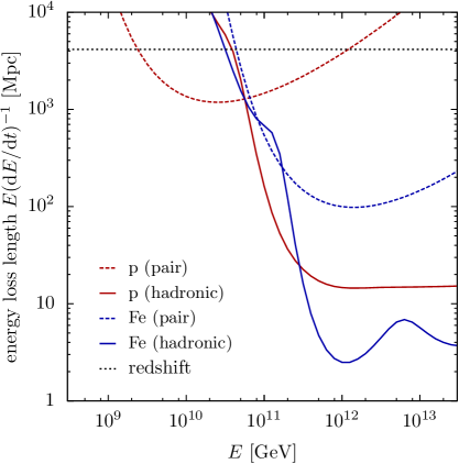
Figure 1: Energy loss length of $e^{+}e^{-}$ pair production (for proton and ⁵⁶Fe nuclei), photopion production, ⁵⁶Fe photodisintegration, and cosmological redshift.

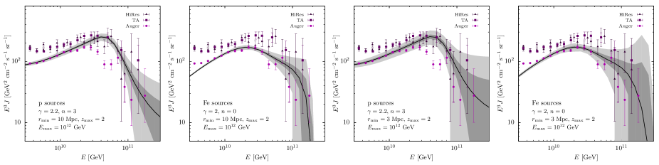
Figure 2: Approximate variation of the flux assuming a local source distribution ${\cal H}_{0}=10^{-5}\leavevmode\nobreak\ {\rm Mpc}^{-3}$ (dark gray band) ${\cal H}_{0}=10^{-6}\leavevmode\nobreak\ {\rm Mpc}^{-3}$ (light gray band) for different assumptions about primary species, emission spectral index $\gamma$, source evolution with redshift $(1+z)^{n}$, and $r_{\min}$. For the energy cuttof at the source, we have taken $E_{\rm max}=10^{12}\leavevmode\nobreak\ {\rm GeV}$.

We want to study the statistical mean and variation of the aggregated flux of $n_{s}$ local sources $N_{A,i}\equiv\sum_{s=1}^{n_{s}}F_{A,i}(r_{s})$. Consider $n_{s}$ sources distributed between redshift $r_{\rm min}$ and $r_{\rm max}$. The number of sources can be expressed via a local source density $\mathcal{H}_{0}$ as $n_{s}=\mathcal{H}_{0}(4\pi/3)(r_{\rm max}^{3}-r_{\rm min}^{3})$. The probability distribution function for a single source is $p(r)=\frac{\mathcal{H}_{0}}{n_{s}}4\pi r^{2}\Theta(r-r_{\rm min})\Theta(r_{\rm max}-r)$.

The ensemble-average of a quantity $X(r_{1},\ldots,r_{n_{s}})$, which depends on the distances of $n_{s}$ sources can be expressed as $\langle X\rangle=\int{\rm d}r_{1}\cdot\ldots\cdot{\rm d}r_{n_{s}}p(r_{1})\cdot\ldots\cdot p(r_{n_{s}})X.$ Therefore, the ensemble-average of the local flux of particle species $A$ is given by $\langle N_{A,i}\rangle\equiv\mathcal{H}_{0}\int_{r_{\rm min}}^{r_{\rm max}}{\rm d}r^{\prime}4\pi r^{\prime 2}F_{A,i}(r^{\prime})$. The mean total flux is obtained by summing over all particle species $\langle N_{\rm tot}(E)\rangle\equiv\sum_{A}\langle N_{A}(E/A)\rangle$. Now, defining the residual $\delta X\equiv X-\left<X\right>$, we can write the covariance between the relative flux of two particle species $A,B$ populating energy bins $i,j$ : $\langle\delta N_{A,i}\delta N_{B,j}\rangle\equiv\langle N_{A,i}N_{B,j}\rangle-\langle N_{A,i}\rangle\langle N_{B,j}\rangle$. The relative variation of the total flux is described by two-point density perturbations

$$\sigma^{2}_{\rm loc}=\sum_{A,B}\frac{\langle\delta N_{A}(E/A)\delta N_{B}(E/B)\rangle}{\langle N_{\rm tot}(E)\rangle^{2}}.$$ (2)

$\sigma^{2}_{\rm loc}$ is the ensemble fluctuation, the sensitivity to which we are interested in exploring for the case of JEM-EUSO.

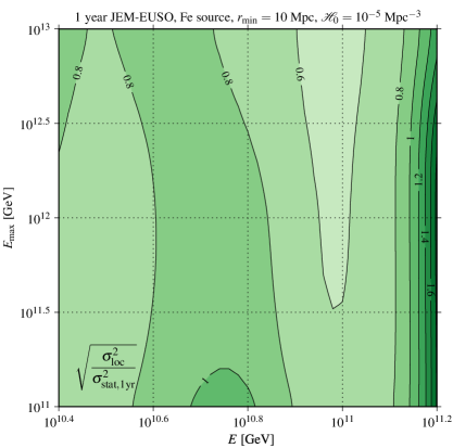
Figure 3: Contours of the ratio between the local relative error of the flux for a distribution of iron sources and the statistics to be collected by JEM-EUSO in one year. For the contour at 1, the statistical error equals the ensemble fluctuation (i.e. the cosmic variance is evident in the energy spectrum).

3 Comparisons with recent data

It is illustrative to compare the size and structure of ensemble fluctuation to recent measurements. In Fig. 2, we show recent data from HiRes [1], Auger [3] and the Telescope Array (TA) [15] compared to the predictions derived from Eq. (2) combined with a modification for a redshift scaling out to $z=2$, as discussed in [6]. The solid line shows the average energy spectrum predicted for certain assumed parameters, which are indicated in the figures. The dark gray band envelopes the ensemble fluctuation for a uniform source density of ${\cal H}_{0}=10^{-5}\leavevmode\nobreak\ {\rm Mpc}^{-3}$, while the lighter band corresponds to ${\cal H}_{0}=10^{-6}\leavevmode\nobreak\ {\rm Mpc}^{-3}$ [16, 17]. The left two figures correspond to the predictions for proton and iron, respectively, under the assumption that $r_{\rm min}=10$ Mpc [18]. The right two figures illustrate the situation for the case of $r_{\rm min}=3$ Mpc. Note the striking dependence of the size of the ensemble fluctuation on the proximity of the nearest source. In fact, the rightmost figure indicates that for the case of iron primaries, the ensemble fluctuation could even allow for a distinctive upward wiggle in the spectrum before the GZK cutoff causes it to plummet. (Candidate nearby sources of heavy nuclei include starburst galaxies [19] and ultra-fast spinning newly-born pulsars [20, 21].)

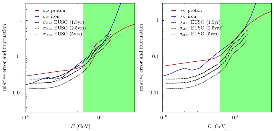
Figure 4: The relative error on the flux is compared to the statistical fluctuation for various integrated exposures for a slice through the contours in Fig 3 at $E_{\rm max}=10^{12}$ GeV. The left panel corresponds to the case of $r_{\rm min}=10$ Mpc while the right panel corresponds to $r_{\rm min}=3$ Mpc. The green shaded region is intended only to draw the reader’s eye to the high energy region of the spectrum, where ensemble fluctuations are the largest.

4 JEM-EUSO discovery reach

From Fig. 2, it is evident that current volume of data at the highest energies is not sufficient to disentangle the ensemble fluctuation phenomenon from statistical fluctuations. Now we consider whether the JEM-EUSO mission will attain sufficient exposure during its projected lifetime to identify ensemble fluctuations for certain assumptions about the source distribution and primary composition.

The Pierre Auger Observatory is currently the world’s largest CR detector. Between 1 January 2004 and 31 December 2010 the observatory collected an integrated exposure of ${\cal E}=20,905\leavevmode\nobreak\ {\rm km}^{2}\,{\rm sr}\,{\rm yr}$ [3]. For the JEM-EUSO baseline design, a factor of 9 increase in annual exposure above $9\times 10^{10}\leavevmode\nobreak\ {\rm GeV}$ is expected. To project the resulting JEM-EUSO event rate, we scale the latest published Auger energy spectrum [3] according to the relative exposure between the Auger Observatory and JEM-EUSO [11].

From this estimate of JEM-EUSO statistics, we find the expected ratio of the ensemble to statistical fluctuations, $\sqrt{\sigma^{2}_{\rm loc}/\sigma^{2}_{\rm stat}}$. Figure 3 contains a contour of this ratio in the plane of the maximum energy attained at the source, $E_{\rm max}$ vs. the observed energy $E$. The precipitous rise in this ratio in the region of extremely high energy is clearly evident.

Finally, in Fig. 4 we display $\sqrt{\sigma^{2}_{\rm loc}}$ for the case of $E_{\rm max}=10^{12}$ GeV compared to statistical uncertainties for various JEM-EUSO exposure times and two different assumptions for $r_{\rm min}$. The solid blue line indicates the relative fluctuation for iron, while the red line corresponds to the proton fluctuation. Note that JEM-EUSO is expected to collect data for at least 3 years, but may attain significantly greater exposure (${\cal E}\approx 5\times 10^{5}\leavevmode\nobreak\ {\rm km}^{2}\,{\rm sr}\,{\rm yr}$) if ISS operations are extended beyond 2020. Figure 4 demonstrates that if the nearest sources are at about 3 Mpc, JEM-EUSO will gather enough statistics in 3 years to make an observation of the ensemble fluctuation. Performing such an observation in two ’realizations’ of the universe, such as the northern and southern skies, or regions of the sky demarcated by anisotropy, will provide a measure of the cosmic variance which is definitive and complementary to direct searches for the CR sources. (It would perhaps be even more interesting to see no variation in the energy spectra of two sky samples.)

5 Conclusions

Ensemble fluctuations are variations in mean energy spectrum predictions reflecting the finite number and distribution of local sources. This phenomenon is one manifestation of the cosmic variance, and provides information complementary to direct searches for the CR emitters. The size and fine details of ensemble fluctuations are sensitive to and therefore yield information about the density of sources, the proximity to the nearest source or source populations, and the composition of the highest energy CRs. When taken together with information on CR clustering on a small angular scale, the size of the ensemble fluctuation may also provide a lower bound on the extragalactic magnetic field.

Ensemble fluctuations persist in the limit of large statistics, and may therefore become evident given a sufficiently large data sample. While current data sets are not large enough to discern these fluctuations, future observatories with huge exposure will afford an opportunity to turn up this phenomenon. Here we have shown that JEM-EUSO will collect sufficient statistics in 3 years of operation to discern ensemble fluctuations manifest in two different samples of the sky if the nearest sources are roughly 3 Mpc away. For more distant sources, at 10 Mpc, 10 years of running will reveal the ensemble fluctuations.

Acknowledgment: We thank Etienne Parizot for some valuable discussion. This work was supported by NASA (11-APRA11-0058 and 11-APRA11-0066) and NSF (CAREER PHY-1053663, PHY-1068696, PHY-1125897, and PHY-1205845).

References

- [1] R. U. Abbasi et al. [HiRes Collaboration], Phys. Rev. Lett. 100, 101101 (2008).
- [2] J. Abraham et al. [Pierre Auger Collaboration], Phys. Rev. Lett. 101, 061101 (2008).
- [3] J. Abraham et al. [Pierre Auger Collaboration], Phys. Lett. B 685, 239 (2010).
- [4] K. Greisen, Phys. Rev. Lett. 16, 748 (1966).
- [5] G. T. Zatsepin and V. A. Kuzmin, JETP Lett. 4, 78 (1966) [Pisma Zh. Eksp. Teor. Fiz. 4, 114 (1966)].
- [6] M. Ahlers, L. A. Anchordoqui and A. M. Taylor, Phys. Rev. D 87, 023004 (2013).
- [7] T. J. Weiler et al., in these proceedings.
- [8] L. A. Anchordoqui, M. T. Dova, L. N. Epele and J. D. Swain, Phys. Rev. D 57, 7103 (1998).
- [9] M. Ahlers and J. Salvado, Phys. Rev. D 84, 085019 (2011).
- [10] J. H. Adams, Jr. et al., arXiv:1203.3451.
- [11] J. H. Adams, Jr. et al. [JEM-EUSO Collaboration], Astropart. Phys. 44, 76 (2013).
- [12] J. Blumer et al. [Pierre Auger Collaboration], New J. Phys. 12, 035001 (2010).
- [13] M. Ahlers and A. M. Taylor, Phys. Rev. D 82, 123005 (2010).o
- [14] P. Abreu et al. [Pierre Auger Collaboration], arXiv:1107.4809.
- [15] T. Abu-Zayyad et al. [Telescope Array Collaboration], arXiv:1205.5067.
- [16] H. Takami, S. Inoue and T. Yamamoto, Astropart. Phys. 35, 767 (2012).
- [17] P. Abreu et al. [Pierre Auger Collaboration], arXiv:1305.1576.
- [18] A. M. Taylor, M. Ahlers and F. A. Aharonian, Phys. Rev. D 84, 105007 (2011).
- [19] L. A. Anchordoqui, G. E. Romero and J. A. Combi, Phys. Rev. D 60, 103001 (1999).
- [20] P. Blasi, R. I. Epstein and A. V. Olinto, Astrophys. J. 533, L123 (2000).
- [21] K. Fang, K. Kotera and A. V. Olinto, Astrophys. J. 750, 118 (2012).