Abstract

We determine the strong coupling constant $\alpha_{s}$ from the $\tau$ hadronic width using a renormalization group summed (RGS) expansion of the QCD Adler function. The main theoretical uncertainty in the extraction of $\alpha_{s}$ is due to the manner in which renormalization group invariance is implemented, and the as yet uncalculated higher order terms in the QCD perturbative series. We show that new expansion exhibits good renormalization group improvement and the behaviour of the series is similar to that of the standard CIPT expansion. The value of the strong coupling in ${\overline{\rm MS}}$ scheme obtained with the RGS expansion is $\alpha_{s}(M_{\tau}^{2})=0.338\pm 0.010$. The convergence properties of the new expansion can be improved by Borel transformation and analytic continuation in the Borel plane. This is discussed elsewhere in these proceedings.

1 Introduction

The inclusive hadronic decay width of the $\tau$ lepton provides a clean source for the determination of $\alpha_{s}$ at low energies [1, 2, 3, 4]. The perturbative QCD contribution is known up to $O(\alpha_{s}^{4})$ [5] and the nonperturbative corrections are found to be small [6, 7, 8, 9, 10, 11]. The main uncertainties arise from the treatment of higher-order corrections and improvement of the perturbative series through renormalization group (RG) methods. The leading methods for the treatment of the perturbative series are fixed-order perturbation theory (FOPT) and contour-improved perturbation theory (CIPT) [12, 13]. The predictions from these methods are not in agreement and the discrepancy between them is one of the main sources of ambiguity in the extraction of $\alpha_{s}$ [9, 11, 14, 15, 16].

The above theoretical discrepancy has been the motivation for proposing an alternative approach. We consider the method developed in [17, 18], using a procedure originally suggested in [19, 20, 21] which we refer to as renormalization-group summation (RGS). This is a framework involving leading logarithms summation, in which terms in powers of the coupling constant and logarithms are regrouped, so that for a given order, the new expansion includes every term in the perturbative series that can be calculated using the RG invariance. The results, which are summarized in this talk, are similar to those in CIPT and predicts $\alpha_{s}$ close to the CIPT prediction [22]. Note that this method was used for the study of the inclusive decays of the b-quark and the hadronic cross section in $e^{+}e^{-}$ annihilation [17, 18]. Our work demonstrates that the method can also be applied with success to the determination of $\alpha_{s}$ from $\tau$ hadronic decays.

It must be noted that the QCD perturbative corrections are also sensitive to as yet uncalculated higher order terms in the series. The coefficients of the perturbative series grow as $n!$ and the series have zero radius of convergence[23, 24, 25, 26]. Consequently one can study the Borel transform of the QCD Adler function which has ultraviolet (UV) and infrared (IR) renormalon singularities in the Borel plane. The divergent behaviour can be considerably tamed by using techniques of series acceleration based on conformal mappings and ‘singularity softening’ [27, 28, 29, 30, 31, 32]. The method is not applicable to the perturbative series in powers of $\alpha_{s}$ since the expanded correlators are singular at $\alpha_{s}=0$, but can be applied in the Borel plane. The large order behaviour of the RGS expansion can be improved using this method [33]. This provides a new class of expansions, which simultaneously implement the RG invariance and the large-order summation by the analytic continuation in the Borel plane. The details may be found elsewhere in these proceedings [34].

2 The QCD Adler function

Our treatment begins with the QCD Adler function, which enters the expression for the total inclusive hadronic width of the $\tau$ lepton. The total inclusive hadronic width of the $\tau$ provides an accurate calculation of the ratio

$$R_{\tau}\,\equiv\,\frac{\Gamma[\tau^{-}\to{\rm hadrons}\,\nu_{\tau}]}{\Gamma[\tau^{-}\to e^{-}\overline{\nu}_{e}\nu_{\tau}]}.$$ (1)

The Cabibbo-allowed combination $R_{\tau,V+A}$ which proceeds through a vector and an axial vector current can be written as

$$R_{\tau,V+A}=S_{\rm EW}|V_{ud}|^{2}\bigg{(}1+\delta^{(0)}+\delta_{\rm EW}+\delta^{(2,m_{q})}_{ud,V/A}+\sum_{D=4,6,\dots}\delta_{ud,V/A}^{(D)}\bigg{)}\,,$$ (2)

where $S_{\rm EW}$ and $\delta_{\rm EW}$ are electroweak corrections, $\delta^{(0)}$ is the dominant universal perturbative QCD correction, and $\delta_{ud}^{(D)}$ denote quark mass and higher $D$-dimensional operator corrections (condensate contributions) arising in the operator product expansion (OPE). Our main interest is in the perturbative correction $\delta^{(0)}$ which can be written as

$$\delta^{{(0)}}=\frac{1}{2\pi i}\!\!\oint\limits_{|s|=M_{\tau}^{2}}\!\!\frac{ds}{s}\left(1-\frac{s}{M_{\tau}^{2}}\right)^{3}\left(1+\frac{s}{M_{\tau}^{2}}\right)\hat{D}_{\rm pert}(s),$$ (3)

where $\hat{D}_{\rm pert}(s)\equiv D^{(1+0)}(s)-1$ is the perturbative part of the reduced function Adler function. The perturbative expansion of $\widehat{D}(s)$ in the “fixed-order perturbation theory” at $\mu^{2}=M_{\tau}^{2}$ reads [9]

$$\widehat{D}_{\rm FOPT}(a_{s},L)=\sum\limits_{n=1}^{\infty}a_{s}^{n}\sum\limits_{k=1}^{n}k\,c_{n,k}\,L^{k-1}\,.$$ (4)

where

$$a_{s}\equiv\alpha_{s}(\mu^{2})/\pi,\quad\quad L\equiv\,\ln(-s/\mu^{2}).$$ (5)

The coefficients $c_{n,1}$ in the ${\overline{\rm MS}}$ scheme for $n_{f}=3$ flavours are (cf. [5] and references therein):

$$c_{1,1}=1,\,c_{2,1}=1.640,\,c_{3,1}=6.371,\,c_{4,1}=49.076.$$ (6)

Several estimates for the next coefficient $c_{5,1}$ are available [8, 9, 11, 16]. The remaining coefficients $c_{n,k}$ for $k>1$ are determined from renormalization-group invariance. The function $\widehat{D}_{\rm pert}$ is scale independent and therefore satisfies the RG equation

$$\mu^{2}\frac{\mathrm{d}}{\mathrm{d}\mu^{2}}\left[\widehat{D}_{\rm pert}(s)\right]=0,$$ (7)

which takes the form

$$\beta(a_{s})\frac{\partial\widehat{D}_{\rm pert}(s)}{\partial a_{s}}-\frac{\partial\widehat{D}_{\rm pert}(s)}{\partial\ln(-s/\mu^{2})}=0,$$ (8)

where

$$\beta(a_{s})\equiv\mu^{2}\frac{\mathrm{d}a_{s}(\mu^{2})}{\mathrm{d}\mu^{2}}=-(a_{s}(\mu^{2}))^{2}\sum_{k=0}^{\infty}\beta_{k}(a_{s}(\mu^{2}))^{k}$$ (9)

is the $\beta$ function. The known $\beta_{j}$ coefficients are [35, 36, 37]:

$$\beta_{0}=9/4,\,\,\beta_{1}=4,\,\,\beta_{2}=10.0599,\,\,\beta_{3}=47.228.$$ (10)

The series (4) is badly behaved especially near the time-like axis due to the large imaginary part of the logarithm $\ln(-s/M_{\tau}^{2})$ along the circle $|s|=M_{\tau}^{2}$ [12, 13]. The choice $\mu^{2}=-s$ provides the CIPT expansion [12, 13]

$$\widehat{D}_{\rm CIPT}(s)=\sum\limits_{n=1}^{\infty}c_{n,1}(a_{s}(-s))^{n}\,,$$ (11)

where the running coupling $a_{s}(-s)$ is determined by solving the renormalization-group equation (9) numerically in an iterative way along the circle, starting with the input value $a_{s}(M_{\tau}^{2})$ at $s=-M_{\tau}^{2}$. This expansion avoids the appearance of large logarithms along the circle $|s|=M_{\tau}^{2}$.

3 Renormalization-Group Summation

The expansion of the Adler function (4) can be written in the RGS form [22, 33]

$$\widehat{D}_{\rm FOPT}(a_{s},L)=\sum_{n=1}^{\infty}a_{s}^{n}D_{n}(a_{s}L),$$ (12)

where the functions $D_{n}(a_{s}L)$, depending on a single variable $u=a_{s}L$, are defined as

$$D_{n}(u)\equiv\sum_{k=n}^{\infty}(k-n+1)c_{k,k-n+1}u^{k-n}.$$ (13)

The function $D_{1}$ sums all the leading logarithms, the second function $D_{2}$ sums the next-to-leading logarithms, and so on. These function can be obtained in a closed analytical form using RG invariance through the equation (8) and the expansion (12). This gives the following RGE equation

$$0 =-\sum_{n=1}^{\infty}\sum_{k=2}^{n}k(k-1)c_{n,k}\,a_{s}^{n}L^{k-2}$$

$$-\left(\beta_{0}a_{s}^{2}+\beta_{1}a_{s}^{3}+\beta_{2}a_{s}^{4}+\ldots+\beta_{l}a_{s}^{l+2}+\ldots\right)\times\sum_{n=1}^{\infty}\sum_{k=1}^{n}nkc_{n,k}a_{s}^{n-1}L^{k-1}.$$ (14)

By extracting the aggregate coefficient of $a_{s}^{n}L^{n-p}$ one obtains the recursion formula $(n\geq p)$

$$0=(n-p+2)c_{n,n-p+2}+\sum_{\ell=0}^{p-2}(n-\ell-1)\beta_{\ell}c_{n-\ell-1,n-p+1}.$$ (15)

Multiplying both sides of (15) by $(n-p+1)u^{n-p}$ and summing from $n=p$ to $\infty$, we obtain a set of first-order linear differential equation for the functions defined in (13) for $n\geq 1$:

$$\frac{\mathrm{d}D_{n}}{\mathrm{d}u}+\sum_{\ell=0}^{n-1}\beta_{\ell}\left(u\frac{\mathrm{d}}{\mathrm{d}u}+n-\ell\right)D_{n-\ell}=0,$$ (16)

with the initial conditions $D_{n}(0)=c_{n,1}$ which follow from (13). The solution of the system (16) can be found iteratively in an analytical form. The solutions $D_{n}(u)$ depend on the coupling constant and logarithms. The expressions of $D_{n}(u)$ for $n\leq 4$, written in terms of the coefficients $c_{k,1}$ with $k\leq n$ and $\beta_{j}$ with $0\leq j\leq n-1$, are:

$$D_{1}(u) =\frac{c_{1,1}}{w},\quad\quad\quad w=1+\beta_{0}u,$$

$$D_{2}(u) =\frac{c_{2,1}}{w^{2}}-\frac{\beta_{1}c_{1,1}\ln w}{\beta_{0}w^{2}},$$ (17)

$$D_{3}(u) =\frac{(\beta_{1}^{2}-\beta_{0}\beta_{2})c_{1,1}}{\beta_{0}^{2}w^{2}}+\left[\frac{(-\beta_{1}^{2}+\beta_{0}\beta_{2})c_{1,1}}{\beta_{0}^{2}}+c_{3,1}\right]w^{-3}$$ (18)

$$+\left[-\frac{\beta_{1}(\beta_{1}c_{1,1}+2\beta_{0}c_{2,1})\ln w}{\beta_{0}^{2}}+\frac{\beta_{1}^{2}c_{1,1}\ln^{2}w}{\beta_{0}^{2}}\right]w^{-3}.$$

$$D_{4}(u)=-\frac{(\beta_{1}^{3}-2\beta_{0}\beta_{1}\beta_{2}+\beta_{0}^{2}\beta_{3})c_{1,1}}{2\beta_{0}^{3}}w^{-2}-\left[\frac{\beta_{1}(-\beta_{1}^{2}+\beta_{0}\beta_{2})c_{1,1}}{\beta_{0}^{3}}+\frac{2(-\beta_{1}^{2}+\beta_{0}\beta_{2})c_{2,1}}{\beta_{0}^{2}}\right]w^{-3}$$

$$+\frac{2\beta_{1}(-\beta_{1}^{2}+\beta_{0}\beta_{2})c_{1,1}\ln w}{\beta_{0}^{3}}w^{-3}+\left[\frac{(-\beta_{1}^{3}+\beta_{0}^{2}\beta_{3})c_{1,1}}{2\beta_{0}^{3}}+\frac{2(-\beta_{1}^{2}+\beta_{0}\ \beta_{2})c_{2,1}}{\beta_{0}^{2}}+c_{4,1}\right]w^{-4}$$

$$-\frac{\beta_{1}(-2\beta_{1}^{2}c_{1,1}+3\beta_{0}\beta_{2}c_{1,1}+2\beta_{0}\beta_{1}c_{2,1}+3\beta_{0}^{2}c_{3,1})\ln w}{\beta_{0}^{3}}w^{-4}$$

$$+\frac{\beta_{1}^{2}(5\beta_{1}c_{1,1}+6\beta_{0}c_{2,1})\ln^{2}w}{2\beta_{0}^{3}}w^{-4}-\frac{\beta_{1}^{3}c_{1,1}\ln^{3}w}{\beta_{0}^{3}}w^{-4}.$$

The higher order solutions can be found in Ref. [22]. These expressions are used for computing the perturbative contribution to the hadronic width of the $\tau$ lepton and the subsequent extraction of $\alpha_{s}(M_{\tau}^{2})$.

4 The properties of the RGS expansion

We now discuss the properties of the RGS expansion in the complex momentum plane, along the circle $s=M_{\tau}^{2}\exp(i\theta)$. In Fig. 1, we show the behaviour of the modulus of the Adler function along the circle given by the first $N=5$ terms in the expansions (4), (11) and (12), respectively. In this calculation and below we used the standard value $\alpha_{s}(M_{\tau}^{2})=0.34$, adopted also in previous studies [9, 31]. One may see that the behaviour of the new RGS expansion is similar to that of the CIPT expansion.

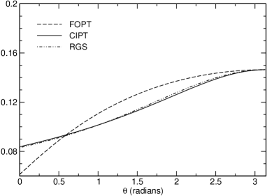
Figure 1: Modulus of the Adler function expansions (4), (11) and (12), summed up to the order $N=5$, along the circle $s=M_{\tau}^{2}\exp(i\theta)$.

In Table 1, we show the values of the quantity $\delta^{(0)}$ defined in (3), calculated with FOPT, CIPT and RGSPT, as a function of the perturbative order up to which the series was summed. We observe that CIPT shows a faster convergence compared to FOPT. To order $N=4$, the difference between FOPT and CIPT is $0.0215$, which is the main source of the theoretical uncertainty in the extraction of $\alpha_{s}$ from the hadronic $\tau$ decay rate. The new RGS expansion, as remarked earlier, shows the convergence which is similar to the CIPT expansion. We note that for $N=4$, the difference between the results of the RGS and the standard FOPT is $0.01754$, and the difference from the RGS and CIPT is $0.0039$, which confirms that the new expansion gives results close to those of the CIPT. For $N=5$, using the estimate $c_{5,1}=283$ from [9], we find that the RGS differs from FOPT by $0.0232$, and from CIPT by $0.0035$.

Table 1: Predictions of $\delta^{(0)}$ by the standard FOPT, CIPT and the RGS, for various truncation orders $N$.

	$\delta^{(0)}_{\rm FOPT}$	$\delta^{(0)}_{\rm CIPT}$	$\delta^{(0)}_{\rm RGS}$
$N=1$	0.1082	0.1479	0.1455
$N=2$	0.1691	0.1776	0.1797
$N=3$	0.2025	0.1898	0.1931
$N=4$	0.2199	0.1984	0.2024
$N=5$	0.2287	0.2022	0.2056

It would be of interest to study the behaviour of RGS expansion at higher orders which are not shown in the Table 1. This is the subject of the next section, in a model for higher order coefficients of the Adler function.

5 Higher order behaviour of the RGS expansion

As discussed earlier, the extraction of $\alpha_{s}$ from the hadronic $\tau$ decays width is also sensitive to the large order behaviour of the QCD perturbative series. It is of interest to check if the low order behaviour of the new RGS expansion persists at higher orders. This investigation was carried out in [22, 33] in a model proposed in [9]. In this model, the RGS expansion of the QCD Adler function has a behaviour which is similar to that of CIPT and eventually exhibits big oscillations, showing the divergent character of the QCD perturbative series at higher orders. In Fig. 2, we show the behaviour of FO, CI and RGS expansions in the so-called “reference model” defined in [9, 38]. The RGS results are close to those of CIPT at every order up to $N=10$. In this model, FOPT expansion approaches better the ‘true value’.

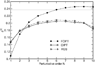
Figure 2: Dependence of $\delta^{(0)}$ in FOPT, CIPT and RGS on the truncation order $N$ in the Beneke and Jamin model [9]. The gray band is the exact value.

A method for taming the divergent behaviour of the QCD perturbative expansions was proposed in [27, 28, 29, 30, 31, 32], using the series acceleration by the conformal mappings of the Borel plane and the implementation of the known nature of the leading singularities in this plane.

In Ref. [33], we applied these techniques to the RGS expansion and defined a novel, RGS non-power (RGSNP) expansion of the QCD Adler function, in which the powers of the coupling of the standard expansion are replaced by suitable functions that resemble the expanded amplitude as concerns their singularities and the expansions in powers of $\alpha_{s}$. The non-power expansions show remarkable convergence properties for the Adler function, which is the crucial input in the determination of $\alpha_{s}$ from hadronic $\tau$ decays. This is reviewed elsewhere in these proceedings [34].

6 Determination of $\alpha_{s}(M_{\tau}^{2})$ from RGS expansion

In this section, we present the derivation of $\alpha_{s}(M_{\tau}^{2})$ following Ref. [22]. We use as input the coefficients $c_{n,1}$ calculated from Feynman diagrams, given in (6), and the estimate $c_{5,1}=283\pm 283$ [9, 16]. We need also the phenomenological value of the pure perturbative correction to the hadronic $\tau$ width, for which we adopt the recent estimate [16],

$$\delta^{(0)}_{\rm phen}=0.2037\pm 0.0040_{exp}\pm 0.0037_{\rm PC},$$ (19)

where the first error is experimental and the second shows the uncertainty due to the power corrections. This value has been used in several recent determinations [30, 16, 31]. With this input we obtain

$$\alpha_{s}(M_{\tau}^{2}) = 0.3378\pm 0.0046_{\rm exp}\pm 0.0042_{\rm PC}~{}^{+0.0062}_{-0.0072}(c_{5,1})$$ (20)

$${}^{+0.0005}_{-0.0004}{(\rm scale)}\pm^{+0.000085}_{-0.000082}{(\rm\beta_{4})}.$$

In the above, the first two errors are due to the corresponding uncertainties of $\delta^{(0)}_{\rm phen}$ given in (19), while the third is due to the uncertainty of the coefficient $c_{5,1}$ with the conservative range adopted above, the fourth is due to scale variation, and the last one is due to the effect of the truncation of the $\beta$-function expansion. The details may be found in [22]. We observe that $\alpha_{s}(M_{\tau}^{2})$ is not sensitive to the variation of the scale. The largest error comes from the uncertainty of the five loop coefficient $c_{5,1}$. This was also observed in the standard CIPT analysis [11, 14] and in the analysis based on the CI expansions improved by the conformal mappings of the Borel plane [30, 31].

Combining in quadrature the errors given in (20), the prediction based on RGS expansion reads [22]

$$\alpha_{s}(M_{\tau}^{2})=0.338\pm 0.010.$$ (21)

We mention that for the same input (19) the standard FOPT and CIPT give, respectively,

$$\alpha_{s}(M_{\tau}^{2}) = 0.320^{+0.012}_{-0.007},\quad\quad\quad{\rm FOPT},$$

$$\alpha_{s}(M_{\tau}^{2}) = 0.342\pm 0.012,\quad\quad{\rm CIPT}.$$ (22)

For comparison we mention also the value $\alpha_{s}(M_{\tau}^{2})=0.320^{+0.019}_{-0.014}$, obtained recently in Ref. [31] with the same input (19) and the CI non-power (CINP) expansion and the value $\alpha_{s}(M_{\tau}^{2})=0.319~{}^{+0.015}_{-0.012}$ determined by the RGS non-power (RGSNP) expansion in the Ref. [33] based on the analytic continuation in the Borel plane. After evolving to the scale of $M_{Z}$, the RGSNP prediction of $\alpha_{s}$ reads $\alpha_{s}(M_{Z}^{2})=0.1184~{}^{+0.0018}_{-0.0015}$. The special features of this latter expansion will be discussed elsewhere in these proceedings [34].

7 Conclusion

In this talk, we have presented our recent results on the determination of the strong coupling constant $\alpha_{s}$ from the $\tau$ hadronic width, based on the formalism which we denote as RGS expansion of the Adler function. Due to the present discrepancy in the determination of the $\alpha_{s}$ from hadronic $\tau$ decays, any alternative approach besides FOPT and CIPT, must be pursued. It must, however, be noted that the RGS framework is an important framework, which was simply not explored in detail earlier in the context of the hadronic decay of the $\tau$ lepton. Our work fills this gap. The method discussed in this talk exploits RG invariance in a complete way, providing analytical closed form solutions to a definite order. The truncated summation of the perturbative series differ among each other by terms of the order $\alpha_{s}^{N+1}$. This difference turns out to be quite important for the low scale relevant in $\tau$ decays.

We have discussed in detail the properties of the RGS expansion, including its properties in the complex energy plane and concluded that these properties are similar to those of CIPT expansion. We also provide the value of the strong coupling $\alpha_{s}$ from this expansion, which is closer to CIPT prediction. We conclude that the the summation of leading logarithms provides a systematic expansion with good convergence properties in the complex plane, including the critical region near the time-like region.

The determination of $\alpha_{s}$ is also ambiguous due to the effect of the as yet uncalculated higher order terms in the perturbative expansion of the hadronic width. This ambiguity is amplified by the fact that the perturbative series is divergent, the coefficients displaying a factorial increase. In QCD, due to the presence of the UV and IR renormalon singularities situated on the real axis in the Borel plane, the Borel-Laplace integral giving the expanded correlators in terms of their Borel transform requires a prescription. Using the Principal Value prescription and the technique of series acceleration by conformal mappings and singularity softening in the Borel plane developed in [27] - [32], we have defined in [33] a new kind of expansion, referred to as RGS non-power (RGSNP) expansion. The divergent behaviour of the standard perturbative series is considerably tamed in the non-power expansions, which show good convergence in the complex energy plane. More details may be found in Refs. [33, 34].

References

- [1] J. Beringer et al. (Particle Data Group), Phys. Rev. D86, 010001 (2012).
- [2] A. Pich, Review of determinations, arXiv:1303.2262.
- [3] M. Jamin,Determination of from tau decays, arXiv:1302.2425.
- [4] G. Altarelli,The QCD Running Coupling and its Measurement, arXiv:1303.6065.
- [5] P.A. Baikov, K.G. Chetyrkin and J.H. Kühn, Phys. Rev. Lett. 101, 012002 (2008), arXiv:0801.1821.
- [6] E. Braaten, S. Narison and A. Pich, Nucl. Phys. B 373, 581 (1992).
- [7] M. Davier, A. Höcker and Z. Zhang, Rev. Mod. Phys. 78, 1043 (2006), hep-ph/0507078.
- [8] M. Davier, S. Descotes-Genon, A. Höcker, B. Malaescu and Z. Zhang, Eur. Phys. J. C56, 305 (2008), arXiv:0803.0979.
- [9] M. Beneke and M. Jamin, JHEP 09, 044 (2008), arXiv:0806.3156.
- [10] A. Pich, Acta Phys. Polon. Supp. 3, 165 (2010), arXiv:1001.0389.
- [11] A. Pich, Tau decay determination of the QCD coupling, in Workshop on Precision Measurements of , ed. S. Bethke et al, page 21, arXiv:1110.0016.
- [12] A.A.Pivovarov, Z. Phys. C 53, 461 (1992), [Sov. J. Nucl. Phys. 54, 676 (1991)] [Yad. Fiz. 54, 1114 (1991)]; hep-ph/0302003.
- [13] F. Le Diberder and A. Pich, Phys. Lett. B 286, 147 (1992).
- [14] A. Pich, Nucl. Phys. B Proc. Suppl., 218, 89 (2011), arXiv:1101.2107.
- [15] S. Bethke, Eur. Phys. J. C64, 689 (2009), arXiv:0908.1135.
- [16] M. Beneke and M. Jamin, Fixed-order analysis of the hadronic decay width, in Workshop on Precision Measurements of , ed. S. Bethke et al, page 25, arXiv:1110.0016.
- [17] M.R. Ahmady, F.A. Chishtie, V. Elias, A.H. Fariborz, N. Fattahi, D.G.C. McKeon, T.N. Sherry, T.G. Steele, Phys. Rev. D 66, 014010 (2002), hep-ph/0203183.
- [18] M.R. Ahmady, F.A. Chishtie, V. Elias, A.H. Fariborz, D.G.C. McKeon, T.N. Sherry, A. Squires, T.G. Steele, Phys. Rev. D 67, 034017 (2003), hep-ph/0208025.
- [19] C.J. Maxwell and A. Mirjalili, Nucl.Phys. B577, 209 (2000), hep-ph/0002204.
- [20] C.J. Maxwell, Nucl.Phys.Proc.Suppl. 86, 74 (2000).
- [21] C.J. Maxwell and A. Mirjalili, Nucl.Phys. B611, 423 (2001), hep-ph/0103164.
- [22] G. Abbas, B. Ananthanarayan and I. Caprini, Phys. Rev. D 85, 094018 (2012), arXiv:1202.2672.
- [23] A.H. Mueller, Nucl. Phys. B 250, 327 (1985).
- [24] A.H. Mueller, in QCD - Twenty Years Later, Aachen 1992, edited by P. Zerwas and H. A. Kastrup (World Scientific, Singapore, 1992).
- [25] D. Broadhurst, Z. Phys. C 58, 339 (1993).
- [26] M. Beneke, Nucl. Phys. B 405, 424 (1993).
- [27] I. Caprini and J. Fischer, Phys. Rev. D 60, 054014 (1999), hep-ph/9811367.
- [28] I. Caprini and J. Fischer, Phys. Rev. D 62, 054007 (2000), hep-ph/0002016.
- [29] I. Caprini and J. Fischer, Eur. Phys. J. C 24, 127 (2002), hep-ph/0110344.
- [30] I. Caprini and J. Fischer, Eur. Phys. J. C64, 35 (2009), arXiv:0906.5211.
- [31] I. Caprini and J. Fischer, Phys. Rev. D 84, 054019 (2011), arXiv:1106.5336.
- [32] I. Caprini and J. Fischer, Nucl. Phys. B Proc. Suppl., 218, 128 (2011), arXiv:1011.6480.
- [33] G. Abbas, B. Ananthanarayan, I. Caprini and J. Fischer, Phys. Rev. D 87, 014008 (2013), arXiv:1211.4316.
- [34] I. Caprini, in this issue of Mod. Phys. Lett. A.
- [35] S.A. Larin, T. van Ritbergen and J.A.M. Vermaseren, Phys. Lett. B400, 379 (1997), hep-ph/9701390.
- [36] S.A. Larin, T. van Ritbergen and J.A.M. Vermaseren, Phys. Lett. B404, 153 (1997),hep-ph/9702435.
- [37] M. Czakon, Nucl. Phys. B710, 485 (2005),hep-ph/0411261.
- [38] M. Beneke, D. Boito and M. Jamin, JHEP 1301, 125 (2013), arXiv:1210.8038.
- [39] D. Boito, M. Golterman, M. Jamin, A. Mahdavi, K. Maltman, J. Osborne and S. Peris, Phys. Rev. D 85, 093015 (2012), arXiv:1203.3146.