Detectability of communities in heterogeneous networks

Abstract

Communities are fundamental entities for the characterization of the structure of real networks. The standard approach to the identification of communities in networks is based on the optimization of a quality function known as “modularity”. Although modularity has been at the center of an intense research activity and many methods for its maximization have been proposed, not much it is yet known about the necessary conditions that communities need to satisfy in order to be detectable with modularity maximization methods. Here, we develop a simple theory to establish these conditions, and we successfully apply it to various classes of network models. Our main result is that heterogeneity in the degree distribution helps modularity to correctly recover the community structure of a network and that, in the realistic case of scale-free networks with degree exponent $\gamma<2.5$, modularity is always able to detect the presence of communities.

Communities are organizational modules that provide a coarse grained view of a complex network Girvan and Newman (2002); Radicchi et al. (2004); Fortunato (2010). Depending on the nature of the network, communities can have different yet fundamental meanings: in biological networks, communities are likely to group entities having the same biological function Spirin and Mirny (2003); Huberman04 ; Guimerà and Amaral (2005), in the graph of the World Wide Web they may correspond to groups of pages dealing with the same or related topics Dourisboure et al. (2009), in food webs they may identify compartments Stouffer et al. (2012), etc. Since communities play an important role for the characterization of the structure of networks, the development of computer algorithms for the detection of communities in networks represents one of the most active areas in network science Fortunato (2010). In particular, the use of the so-called “modularity” has attracted a great attention in recent years Newman and Girvan (2004); Newman (2006). Modularity is a quality function that estimates the relevance of a given network partition (i.e., a division of the network in a given set of communities) by comparing the observed number of internal connections of the communities with the expected number of such edges in a random annealed version of the network. The best community division of the network is then given by the partition that maximizes the modularity function.
Although subjected to some intrinsic limitations Fortunato and Barthélemy (2007); Good (2010), modularity has become a standard tool for community detection and several methods for modularity maximization have been developed Fortunato (2010). In this paper, we focus our attention on spectral optimization of the modularity function, i.e., a maximization method that is essentially based on the determination of the principal eigenpair of the so-called modularity matrix Newman (2006). This represents a way to approximate the configuration corresponding to the maximum of the modularity function, whose determination would be otherwise a NP complete problem Brandes et al. (2008), by relaxing the indices that assign the nodes to the various communities from integer to real valued numbers. This method provides in general solutions that are consistent with those obtained by other more sophisticated maximization techniques Newman (2006); Nadakuditi and Newman (2012), thus the following results can be reasonably considered as valid for any type of community detection algorithm based on modularity maximization.

We consider here the simple case of a symmetric and weighted network formed only by $2$ communities of size $N$. The adjacency matrices that contain the information about the internal structure of these two groups are denoted respectively with $A_{1,1}$ and $A_{2,2}$, while the connections among nodes of different groups are listed in the matrix $A_{1,2}=A_{2,1}^{T}$. The adjacency matrix of the entire network can be thus written in the following block form

$$A=\left(\begin{array}[]{cc}A_{1,1}&A_{1,2}\\ A_{2,1}&A_{2,2}\end{array}\right)\;.$$ (1)

According to the definition of the modularity function, in the random annealed version of the network, which preserves on average the node degrees, the probability that two nodes are connected is proportional to the product of the degrees of the two nodes Molloy and Reed (1995); Newman and Girvan (2004). The entire information of this null model is contained in the square matrix

$$P=\frac{1}{\left<s_{1}|1\right>+\left<s_{2}|1\right>}\left(\begin{array}[]{cc}\left|s_{1}\right>\left<s_{1}\right|&\left|s_{1}\right>\left<s_{2}\right|\\ \left|s_{2}\right>\left<s_{1}\right|&\left|s_{2}\right>\left<s_{2}\right|\end{array}\right)\;,$$

where $\left|s_{i}\right>=\left|s_{i,i}\right>+\left|s_{i,j}\right>$ is the strength vector of the $i$-th group, with $\left|s_{i,j}\right>=A_{i,j}\left|1\right>$ equal to a vector whose components are equal to the sum of the weights of all edges connecting nodes of the $i$-th group to nodes of the $j$-th group, and $\left|1\right>$ is the vector whose components are all equal to one.

Let us focus our attention on the spectrum of the modularity matrix $Q=A-P$ Newman (2006). Note that by definition $Q\left|1\right>=\left|0\right>$, where $\left|0\right>$ is the vector with all components equal to zero, thus any other eigenvector $\left|v\right>$ of the modularity matrix $Q$, i.e., $Q\left|v\right>=\lambda\left|v\right>$, must be orthogonal to the vector $\left|1\right>$. We can rewrite the eigenvector $\left|v\right>=\left|v_{1},v_{2}\right>$, where $\left|v_{i}\right>$ is the part of the eigenvector $\left|v\right>$ that corresponds to the $i$-th group. The orthogonality with respect to the eigenvector $\left|1\right>$ reads $\left<v_{1}|1\right>+\left<v_{2}|1\right>=0$, while the normality of the eigenvector means that $\left<v_{1}|v_{1}\right>+\left<v_{2}|v_{2}\right>=1$. The eigenvalue problem becomes equivalent to

$$A_{1,1}\left|v_{1}\right>+A_{1,2}\left|v_{2}\right>-\frac{\left<s_{1}|v_{1}\right>+\left<s_{2}|v_{2}\right>}{\left<s_{1}|1\right>+\left<s_{2}|1\right>}\left|s_{1}\right>=\lambda\left|v_{1}\right>$$ (2)

and

$$A_{2,2}\left|v_{2}\right>+A_{2,1}\left|v_{1}\right>-\frac{\left<s_{1}|v_{1}\right>+\left<s_{2}|v_{2}\right>}{\left<s_{1}|1\right>+\left<s_{2}|1\right>}\left|s_{2}\right>=\lambda\left|v_{2}\right>\;.$$ (3)

If we multiply them for $\left<1\right|$, and then take their difference, we obtain

$$\begin{array}[]{l}\lambda\left(\left<v_{1}|1\right>-\left<v_{2}|1\right>\right)=\left(\left<s_{1,1}|v_{1}\right>-\left<s_{1,2}|v_{1}\right>\right.\\ \left.-\left<s_{2,2}|v_{2}\right>+\left<s_{2,1}|v_{2}\right>\right)-\alpha\left(\left<s_{1}|v_{1}\right>-\left<s_{2}|v_{2}\right>\right)\end{array}\;,$$ (4)

where we have defined $\alpha=\frac{\left<s_{1}|1\right>-\left<s_{2}|1\right>}{\left<s_{1}|1\right>+\left<s_{2}|1\right>}$. For simplicity, in the following we will consider only cases in which $\alpha\simeq 0$, i.e., cases in which both groups have a comparable total number of edges.

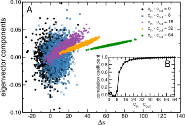
Figure 1: (Color online) A Components of the principal eigenvector of the modularity matrix as functions of the difference between internal and external degrees for a system composed of two poissonian networks of size $N=1024$, with average internal degree $c_{in}$ and average external degree $c_{out}$ such that $c_{in}+c_{out}=64$. We plot here only the components of one of the two modules, but analogous results (with opposite sign) are valid for the other module. Different colors and symbols correspond to different combinations of $c_{in}$ and $c_{out}$. B Correlation coefficient between the eigenvector components and the difference between internal and external degrees as a function of $c_{in}-c_{out}$. While the correlation coefficient is not significant in the region in which communities are not detectable [i.e., $c_{in}-c_{out}<\sqrt{c_{in}+c_{out}}$, see Eq. (12)], it becomes significant in the detectability regime (i.e., $c_{in}-c_{out}\geq\sqrt{c_{in}+c_{out}}$).

We define the detectability regime as the regime in which the two pre-imposed communities can be detected by means of modularity spectral optimization. This regime is characterized by the fact that the components of the principal eigenvector corresponding to the nodes of one of the modules have coherent signs, while the two portions of the eigenvector corresponding to different groups are opposite in sign Newman (2006). If we suppose that these modules are uncorrelated graphs (i.e., without further internal sub-community structure) with prescribed in- and out-strength vectors, we expect that this eigenvector is such that

$$\left|v_{1}\right>=n_{1}\,\left(\left|s_{1,1}\right>-\left|s_{1,2}\right>\right)=n_{1}\left|\Delta s_{1}\right>$$ (5)

and

$$\left|v_{2}\right>=n_{2}\,\left(\left|s_{2,2}\right>-\left|s_{2,1}\right>\right)=n_{2}\left|\Delta s_{2}\right>\;,$$ (6)

where $n_{1}$ and $n_{2}$ are proportionality constants, while $\left|\Delta s_{1}\right>$ and $\left|\Delta s_{2}\right>$ are respectively the vectors whose entries are given by the difference of the in- and out-strengths of the nodes in the groups 1 and 2. Eqs. (5) and (6) simply state that the coordinates of $\left|v_{1}\right>$ and $\left|v_{2}\right>$ are linearly proportional to the difference of the in- and out- strength vectors, a solution that appears natural if we interpret the modularity function as the stationary solution of a random walk between the two communities Lambiotte et al. (2009); Lambiotte (2010); Mucha et al. (2010). This conjecture is indeed perfectly verified in numerical estimations of the largest eigenvector of the modularity matrix (see Figs. 1,S1 and S2), and thus Eqs. (5) and (6) can be used as a reasonable ansazt for the solution of our problem. If we finally insert Eqs. (5) and (6) into Eq. (4), we can give an estimate of the largest eigenvalue $\lambda_{max}$ of the modularity matrix in the regime of detectable communities, and write

$$\lambda_{max}=\frac{1}{2}\left(\frac{\left<\Delta s_{1}|\Delta s_{1}\right>}{\left<\Delta s_{1}|1\right>}+\frac{\left<\Delta s_{2}|\Delta s_{2}\right>}{\left<\Delta s_{2}|1\right>}\right)\;,$$ (7)

where we have used the orthogonality condition $\left<v_{1}|1\right>+\left<v_{2}|1\right>=0$, which leads to $n_{1}=-n_{2}\left<\Delta s_{2}|1\right>/\left<\Delta s_{1}|1\right>$. Note that expression Eq. (7) is valid for given strength vectors. If we instead assume that the entries of these vectors are random variates obeying the statistical distributions $P\left(\Delta s_{1}\right)$ and $P\left(\Delta s_{2}\right)$, we can write

$$\lambda_{max}=\frac{1}{2}\left(\frac{m_{2}^{(1)}}{m_{1}^{(1)}}+\frac{m_{2}^{(2)}}{m_{1}^{(2)}}\right)\;,$$ (8)

where $m_{1}^{(i)}$ and $m_{2}^{(i)}$ are respectively the first and the second moments of the distribution $P\left(\Delta s_{i}\right)$.

It is important to stress that Eqs. (7) and (8) give us an estimate of the largest eigenvalue of $Q$ only in the detectability regime. If the structure of the entire graph is instead such that the two modules are not detectable by means of modularity maximization, there will another principal eigenvector orthogonal to the previous one, and thus not showing the presence of the two modules. Since we have supposed that both modules are randomly generated graphs, the other eigenvalue that is competing with $\lambda_{max}$ for being the highest eigenvalue of the modularity matrix is given by the second largest eigenvalue of the annealed random network associated to $Q$ Nadakuditi and Newman (2012). In intuitive terms, this means that, in the regime in which the groups are undetectable, the signal present in $A$ is not sufficiently high, and $Q$ is in spectral terms indistinguishable from $P$. In the following, we will consider some examples of network ensembles where both these eigenvalues can be analytically estimated, and thus the detectability problem can be explicitly solved.

Regular graphs. In this case, each node has exactly $c_{in}$ random connections with other nodes in its group, and $c_{out}$ random connections outside its own group. Eq. (4) reduces to

$$\begin{array}[]{l}\left(\lambda_{max}-c_{in}+c_{out}\right)\left<v_{1}|1\right>=0\\ \left(\lambda_{max}-c_{in}+c_{out}\right)\left<v_{2}|1\right>=0\end{array}\;,$$ (9)

thus either (i) $\left<v_{1}|1\right>=\left<v_{2}|1\right>=0$ and $\lambda_{max}\neq c_{in}-c_{out}$, or (ii) $\lambda_{max}=c_{in}-c_{out}$, $\left<v_{1}|1\right>\neq 0$ and $\left<v_{2}|1\right>\neq 0$. In case (ii), one can also prove that the only possible solution is $\left|v_{1}\right>=\pm\left|1\right>/\sqrt{2N}$ and $\left|v_{2}\right>=\mp\left|1\right>/\sqrt{2N}$ (see Supplemental Material). The same result can be also obtained using Eq. (8) that reduces to Eq. (9) by setting $P\left(\Delta s_{1}\right)=P\left(\Delta s_{2}\right)=\delta\left(c_{in}-c_{out}\right)$. The term of comparison for $\lambda_{max}$ in the case of regular graphs is given by the second largest eigenvalue of the adjacency matrix of a random regular graph with valency $c=c_{in}+c_{out}$, that is in good approximation equal to $2\sqrt{c}$ Alon (1986); Friedman (2003). Eq. (9) tells us that, independently of the system size, the two modules can be either fully detectable or not detectable at all. The sudden transition between these two regimes happens at the point in which

$$c_{in}-c_{out}=2\sqrt{c_{in}+c_{out}}\;.$$ (10)

This theoretical prediction is in perfect agreement with the results of the numerical simulations reported in Fig. 2.

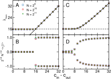
Figure 2: (Color online) Numerical estimation of the largest eigenpair of the modularity matrix $Q$ in the case of two random regular graphs (panels A and B) and in the case of two poissonian graphs (panels C and D). In both cases we consider three different network sizes $N=256$ (blue squares), $N=512$ (red circles) and $N=1024$ (green triangles), and we fix $c_{in}+c_{out}=64$. The results presented here have been obtained by averaging over $100$ different realizations of the models. A and C Largest eigenvalue of $Q$ as a function of $c_{in}-c_{out}$. The full black line corresponds to $c_{in}-c_{out}$ in panel A, and to Eq. (11) in C. The dashed black lines are given by $2\sqrt{c_{in}+c_{out}}$. B and D Size independent inner products $\left<v_{1}|1\right>$ and $\left<v_{2}|1\right>$ as functions of $c_{in}-c_{out}$.

Poissonian networks. This is the case whose entire spectrum has been analytically determined by Nadakuditi and Newman Nadakuditi and Newman (2012). Internal degrees in both groups are drawn from a Poisson distribution with average $c_{in}$, and external degrees are also poissonian variates with average $c_{out}$. In this case, the distributions $P\left(\Delta s_{1}\right)$ and $P\left(\Delta s_{2}\right)$ are two identical Skellam distributions, with first moment equal to $m_{1}=c_{in}-c_{out}$, and second moment equal to $m_{2}=\left(c_{in}+c_{out}\right)+\left(c_{in}-c_{out}\right)^{2}$ Skellam (1946). We can reduce Eq. (8) to

$$\lambda_{max}=c_{in}-c_{out}+\frac{c_{in}+c_{out}}{c_{in}-c_{out}}\;.$$ (11)

This result is identical to the prediction obtained in Nadakuditi and Newman (2012). The term of comparison for the largest eigenvalue of the modularity matrix is given by the second largest eigenvalue of a random graph with average degree $c=c_{in}+c_{out}$, that is $2\sqrt{c}$ Chung et al. (2003a); Nadakuditi and Newman (2012), and this finally leads to the detectability threshold

$$c_{in}-c_{out}=\sqrt{c_{in}+c_{out}}\;,$$ (12)

as already obtained in Decelle et al. (2001); Nadakuditi and Newman (2012). The results of numerical simulations perfectly agree with our theoretical prediction (see Fig. 2). The prediction appears to be not visibly dependent on the system size, and already for small networks Eq. (12) represents a very good estimate of the transition point. We note that, as in the case of regular graphs, for a large portion of the region $c_{in}>c_{out}$ modularity fails to recover the community structure of the graph. It is, however, interesting to stress that the detectability threshold is two times smaller than the one registered for regular graphs, and thus the heterogeneity in node degrees seems to enhance the ability of modularity to detect communities.

LFR benchmark graphs. As a final example, we consider a special case of the benchmark graphs introduced by Lancichinetti et al Lancichinetti et al. (2008). We set $\left|s_{1,1}\right>=\left|s_{2,2}\right>=c_{in}\left|s\right>$ and $\left|s_{1,2}\right>=\left|s_{2,1}\right>=c_{out}\left|s\right>$, where the entries of the vector $\left|s\right>$ are random variates in the range $1$ to $N$ taken from a power-law distribution with exponent $\gamma$. Eq. (8) becomes

$$\lambda_{max}=\left(c_{in}-c_{out}\right)\,\frac{\zeta_{N}\left(\gamma-2\right)}{\zeta_{N}\left(\gamma-1\right)}\;,$$ (13)

where $\zeta_{N}\left(x\right)=\sum_{n=1}^{N}n^{-x}$ is the Riemann zeta function truncated at the $N$-th term. The term of comparison for the largest eigenvalue of the modularity matrix is still given by the second largest eigenvalue of the annealed random graph associated with the modularity matrix. We do not have an exact guess on how this quantity depends on parameters of the network model, but we can use the upper bound of the largest eigenvalue of random scale-free graphs to get more insights. According to the predictions by Chung et al adapted to the present case, the largest eigenvalue $\mu_{max}$ of our random scale-free graphs is equal to the maximum between $\mu_{max}^{(1)}=\left(c_{in}+c_{out}\right)\,\frac{\zeta_{N}\left(\gamma-2\right)}{\zeta_{N}\left(\gamma-1\right)}$ and $\mu_{max}^{(2)}=\sqrt{\left(c_{in}+c_{out}\right)s_{max}}$, with $s_{max}$ largest degree in the network Chung et al. (2003a, b). In the limit of sufficiently large $N$, we have that: for $\gamma<2.5$, the dominating eigenvalue is $\mu_{max}^{(1)}$; for $\gamma>2.5$, the largest eigenvalue is instead $\mu_{max}^{(2)}$. This has very important implications when compared to our prediction of $\lambda_{max}$ given in Eq. (13): (i) For $\gamma<2.5$, $\lambda_{max}$ grows as fast as $\mu_{max}$ with the system size, thus the detectability threshold should approach zero as $N$ increases. (ii) For $\gamma>2.5$ instead, $\mu_{max}$ grows faster than $\lambda_{max}$ as $N$ increases. The detectability threshold should grow with the system size, and eventually converge to a finite fixed value (for instance, for $\gamma\to\infty$ we must recover the result valid for the case of regular graphs).
The results of numerical simulations support our thesis (see Fig. 3). When we plot $\lambda_{max}\frac{q_{1}}{q_{2}}$ as a function of $c_{in}-c_{out}$, with $q_{1}$ and $q_{2}$ respectively the first and second moments of the strength distribution of the network, we see that when $\gamma<2.5$ this quantity slowly approaches, as $N$ increases, the linear behavior $c_{in}-c_{out}$ as predicted by Eq. (13). This means that, in the limit of infinite large systems, modularity is able to detect the presence of the network blocks for every $c_{in}>c_{out}$. Instead, for $\gamma>2.5$, the lower part of the curve tends to move away from the linear behavior as the system size grows. This implies that there will be, also in the limit of infinitely large systems, always a part of the $c_{in}>c_{out}$ region in which the two blocks are undetectable via modularity maximization.

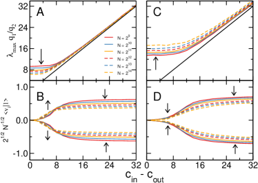
Figure 3: (Color online) Numerical estimation of the largest eigenpair of the modularity matrix $Q$ in the case of two random scale-free graphs with degree exponents $\gamma=2.2$ (panels A and B) and $\gamma=2.8$ (panels C and D). In both cases, we consider several network sizes ranging from $N=256$ to $N=8192$, and we set $c_{in}+c_{out}=64$. The results presented here have been obtained by averaging over $100$ different realizations of the models. To suppress fluctuations, we restricted to the case of networks for which the square of the largest strength is smaller than the sum of all strengths (i.e., $s_{max}^{2}<\sum_{i}s_{i}$) Chung et al. (2003a, b), although the qualitative outcome does not depend on this choice. For clarity, we placed arrows in the various panels to indicate the direction of increasing $N$. A and C Largest eigenvalue $\lambda_{max}$ multiplied by $q_{1}/q_{2}$ as a function of $c_{in}-c_{out}$. The full black line corresponds to $c_{in}-c_{out}$. B and D Size independent inner products $\left<v_{1}|1\right>$ and $\left<v_{2}|1\right>$ as functions of $c_{in}-c_{out}$.

To summarize, we identified the necessary conditions that communities need to satisfy in order to be detectable by means of modularity maximization. Our results are valid for the case of $2$ groups with comparable number of edges, and when the information about the number of such groups is used as ingredient in the maximization of the modularity function. Our main result is that in random network ensembles with pre-imposed community structure, the eigenvector of the modularity matrix that identifies the presence of the block structure is associated with an eigenvalue approximately equal to the ratio between the second and the first moments of the distribution of the difference between internal and external node strengths. If this eigenvalue is larger than the second largest eigenvalue of the null model associated to the modularity function, then modularity is able to detect such a structure, otherwise not. This represents a limitation in the case of graphs with homogeneous degrees. Increasing the heterogeneity of the network accelerates instead the ability of modularity to recover the correct community structure. For example, adding noise to a regular graph makes the detectability threshold two times smaller. More importantly, if the heterogeneity of the node degrees is sufficiently high, as in the case of real networked systems, then modularity is always able to detect communities.

Supplemental Material

Principal eigenpair of the modularity matrix for regular graphs

For regular graphs, we have

$$\left|s_{1}\right>=\left|s_{2}\right>=(c_{in}-c_{out})\left|1\right>\;,$$

thus

$$\left<s_{1}|v_{1}\right>+\left<s_{2}|v_{2}\right>=(c_{in}-c_{out})\left(\left<1|v_{1}\right>+\left<1|v_{2}\right>\right)=0$$

for the orthogonality of the eigenvector $\left|v_{1},v_{2}\right>$ with respect to the vector $\left|1\right>$, and Eqs.(2) and (3) of the main text reduce to

$$A_{1,1}\left|v_{1}\right>+A_{1,2}\left|v_{2}\right>=\lambda\left|v_{1}\right>$$ (S1)

and

$$A_{2,2}\left|v_{2}\right>+A_{2,1}\left|v_{1}\right>=\lambda\left|v_{2}\right>\;.$$ (S2)

Consider the eigenvalue $\lambda=c_{in}-c_{out}$ (which corresponds to the principal eigenvalue of the modularity matrix in the case of detectable communities, as proved in the main text). The only term on the l.h.s. of Eq. (S1) that depends on $c_{in}$ is $A_{1,1}\left|v_{1}\right>$, while the only term that depends on $c_{out}$ is $A_{1,2}\left|v_{2}\right>$. This means that Eq. (S1) can be decoupled in two equations

$$A_{1,1}\left|v_{1}\right>=c_{in}\left|v_{1}\right>\qquad\textrm{ and }\qquad A_{1,2}\left|v_{2}\right>=-c_{out}\left|v_{1}\right>\;.$$ (S3)

Similarly, Eq. (S2) leads to

$$A_{2,2}\left|v_{2}\right>=c_{in}\left|v_{2}\right>\qquad\textrm{ and }\qquad A_{2,1}\left|v_{1}\right>=-c_{out}\left|v_{2}\right>\;.$$ (S4)

Since the subgraphs encoded by the adjacency matrices $A_{1,1}$ and $A_{2,2}$ are regular graphs with valency $c_{in}$, this means that $\left|v_{1}\right>=n_{1}\left|1\right>$ and $\left|v_{2}\right>=n_{2}\left|1\right>$, with $n_{1}$ and $n_{2}$ suitable normalization constants. The same consideration is valid also for the subgraph encoded by the adjacency matrix $A_{1,2}=A_{2,1}$ which is still a regular graph (with valency $c_{out}$ in this case) and thus Eq. (S3) and (S4) consistently lead to the same solutions $\left|v_{1}\right>=n_{1}\left|1\right>$ and $\left|v_{2}\right>=n_{2}\left|1\right>$. Since the eigenvector $\left|v_{1},v_{2}\right>$ is orthogonal to the vector $\left|1\right>$ (i.e, $\left<v_{1}|1\right>+\left<v_{2}|1\right>=0$) and properly normalized (i.e., $\left<v_{1}|v_{1}\right>+\left<v_{2}|v_{2}\right>=1$), one finally finds that $n_{1}=-n_{2}=\pm 1/\sqrt{2N}$.

Numerical estimation of the principal eigenpair of the modularity matrix for LFR benchmark graphs

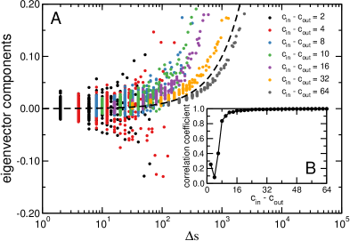
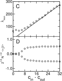
Figure S1: Numerical estimation of the largest eigenpair of the modularity matrix $Q$ for a single realization of two random scale-free graphs with degree exponent $\gamma=2.2$, size $N=1024$, and internal and external degree parameters such that $c_{in}+c_{out}=64$. A Components of the principal eigenvector as functions of the difference between internal and external degrees. We plot here only the components of one of the two modules, but analogous results (with opposite sign) are valid for the other module. Different colors corresponds to different combinations of $c_{in}$ and $c_{out}$. The black dashed line is proportional to $c_{in}-c_{out}$. B Correlation coefficient between the eigenvector components and the difference between internal and external degrees as a function of $c_{in}-c_{out}$. C Largest eigenvalue of $Q$ as a function of $c_{in}-c_{out}$. The full black line corresponds to $(c_{in}-c_{out})\frac{q_{2}}{q_{1}}$, where $q_{2}/q_{1}=8.55$ in the case of this specific model realization. D Size independent inner products $\left<v_{1}|1\right>$ and $\left<v_{2}|1\right>$ as functions of $c_{in}-c_{out}$.

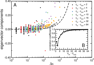
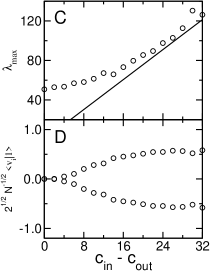
Figure S2: Numerical estimation of the largest eigenpair of the modularity matrix $Q$ for a single realization of two random scale-free graphs with degree exponent $\gamma=2.8$, size $N=1024$, and internal and external degree parameters such that $c_{in}+c_{out}=64$. A Components of the principal eigenvector as functions of the difference between internal and external degrees. We plot here only the components of one of the two modules, but analogous results (with opposite sign) are valid for the other module. Different colors corresponds to different combinations of $c_{in}$ and $c_{out}$. The black dashed line is proportional to $c_{in}-c_{out}$. B Correlation coefficient between the eigenvector components and the difference between internal and external degrees as a function of $c_{in}-c_{out}$. C Largest eigenvalue of $Q$ as a function of $c_{in}-c_{out}$. The full black line corresponds to $(c_{in}-c_{out})\frac{q_{2}}{q_{1}}$, where $q_{2}/q_{1}=3.79$ in the case of this specific model realization. D Size independent inner products $\left<v_{1}|1\right>$ and $\left<v_{2}|1\right>$ as functions of $c_{in}-c_{out}$.

References

Girvan and Newman (2002)
M. Girvan and
M. E. J. Newman,
Proc. Natl. Acad. Sci. USA 99,
7821 (2002).
Radicchi et al. (2004)
F. Radicchi,
C. Castellano,
F. Cecconi,
V. Loreto, and
D. Parisi,
Proc. Natl. Acad. Sci. USA 101,
2658 (2004).
Fortunato (2010)
S. Fortunato,
Phys. Rep. 486,
75 (2010).
Spirin and Mirny (2003)
V. Spirin and
L. Mirny,
Proc. Natl. Acad. Sci. USA 100,
12123 (2003).
(5)
D. M. Wilkinson and
B. A. Huberman,
Proc. Natl. Acad. Sci. USA 101,
5241 (2004).
Guimerà and Amaral (2005)
R. Guimerà and
L. A. N. Amaral,
Nature 433,
895 (2005).
Dourisboure et al. (2009)
Y. Dourisboure,
F. Geraci, and
M. Pellegrini,
ACM Trans. Web 3,
1 (2009).
Stouffer et al. (2012)
D. B. Stouffer,
M. Sales-Pardo,
M. I. Sirer, and
J. Bascompte,
Science 335,
1489 (2012).
Newman and Girvan (2004)
M. E. J. Newman
and M. Girvan,
Phys. Rev. E 69,
026113 (2004).
Newman (2006)
M. E. J. Newman,
Proc. Natl. Acad. Sci. USA 103,
8577 (2006).
Fortunato and Barthélemy (2007)
S. Fortunato and
M. Barthélemy,
Proc. Natl. Acad. Sci. USA 104,
36 (2007).
Good (2010)
B. H. Good,
Y. A. de Montjoye
and
A. Clauset,
Phys. Rev. E 81,
046106 (2010).
Brandes et al. (2008)
U. Brandes,
D. Delling,
M. Gaertler,
R. Görke,
M. Hoefer,
Z. Nikoloski,
and D. Wagner,
IEEE T. Knowl. Data En. 20,
172 (2008).
Nadakuditi and Newman (2012)
R. R. Nadakuditi
and M. E. J.
Newman, Phys. Rev. Lett.
108, 188701
(2012).
Molloy and Reed (1995)
M. Molloy and
B. Reed,
Random Struct. Algor. 6,
161 (1995).
Lambiotte et al. (2009)
R. Lambiotte,
J. C. Delvenne,
and M. Barahona,
arXiv:0812.1770 (2009).
Lambiotte (2010)
R. Lambiotte, in
WiOpt (IEEE,
2010), pp. 546–553.
Mucha et al. (2010)
P. J. Mucha,
T. Richardson,
K. Macon,
M. A. Porter,
and J.-P.
Onnela, Science
328, 876 (2010).
Alon (1986)
N. Alon,
Combinatorica 6,
83 (1986).
Friedman (2003)
J. Friedman, in
Stoc ’03 (ACM,
2003), pp. 720–724.
Skellam (1946)
J. G. Skellam,
J. R. Stat. Soc. 109,
296 (1946).
Chung et al. (2003a)
F. Chung,
L. Lu, and
V. Vu, Proc.
Natl. Acad. Sci. USA 100, 6313
(2003a).
Decelle et al. (2001)
A. Decelle,
F. Krzakala,
C. Moore, and
L. Zdeborová,
Phys. Rev. Lett. 107,
065701 (2001).
Lancichinetti et al. (2008)
A. Lancichinetti,
S. Fortunato,
and F. Radicchi,
Phys. Rev. E 78
(2008).
Chung et al. (2003b)
F. Chung,
L. Lu, and
V. Vu, Ann.
Comb. 7, 21
(2003b).