Asymptotic theory with hierarchical autocorrelation: Ornstein–Uhlenbeck tree models

Abstract

Hierarchical autocorrelation in the error term of linear models arises when sampling units are related to each other according to a tree. The residual covariance is parametrized using the tree-distance between sampling units. When observations are modeled using an Ornstein–Uhlenbeck (OU) process along the tree, the autocorrelation between two tips decreases exponentially with their tree distance. These models are most often applied in evolutionary biology, when tips represent biological species and the OU process parameters represent the strength and direction of natural selection. For these models, we show that the mean is not microergodic: no estimator can ever be consistent for this parameter and provide a lower bound for the variance of its MLE. For covariance parameters, we give a general sufficient condition ensuring microergodicity. This condition suggests that some parameters may not be estimated at the same rate as others. We show that, indeed, maximum likelihood estimators of the autocorrelation parameter converge at a slower rate than that of generally microergodic parameters. We showed this theoretically in a symmetric tree asymptotic framework and through simulations on a large real tree comprising 4507 mammal species.

T1Supported in part by the NSF Grants DEB-0830036 and DMS-11-06483.

and

Lam Si Tung Ho, Cecile Ane

1 Introduction and overview of main results

1.1 Motivation

This work is motivated by the availability of very large data sets to compare biological species, and by the current lack of asymptotic theory for the models that are used to draw inference from species comparisons. For instance, Cooper and Purvis (2010) studied the evolution of body size in mammals using data from 3473 species whose genealogical relationships are depicted by their family tree in Figure 1. Even from this abundance of data, Cooper and Purvis found a lack of power to discriminate between a model of neutral evolution versus a model with natural selection.

Figure 1: Family tree of 4507 mammal species [Bininda-Emonds et al. (2007)]. Branch lengths indicate estimated diversification times on the horizontal axis. The Cretaceous/Tertiary mass extinction event marked the extinction of dinosaurs 65.5 million years ago. Cooper and Purvis (2010) used body mass data available for 77% of these species to infer the mode of evolution: neutral evolution (BM) versus natural selection (OU).

To model neutral evolution, body size is assumed to follow a Brownian motion (BM) along the branches of the tree, with observations made on present-day species at the tips of the tree. To model natural selection, body size is assumed to follow an Ornstein–Uhlenbeck (OU) process, whose parameters represent a selective body size ($\mu$) and a selection strength ($\alpha$). The lack of power observed by Cooper and Purvis suggests a nonstandard asymptotic behavior of the model parameters, which is the motivation for our work.

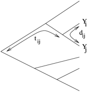
Figure 2: Correlation (or residual correlation) between observations at tips $i$ and $j$ are parametrized in the OU model as a function of the tree distance $d_{ij}$ between $i$ and $j$ and of the length $t_{ij}$ of their shared path from the root. For instance, Cooper and Purvis (2010) considered body mass ($Y$) across 3473 mammal species ($i,j=1,\ldots,3473$).

1.2 Tree structured autocorrelation

Hierarchical autocorrelation, as depicted in the mammalian tree, arises whenever sampling units are related to each other through a vertical inheritance pattern, like biological species, genes in a gene family or human cultures. In the genealogical tree describing the relatedness between units, internal nodes represent ancestral unobserved units (like species or human languages). Branch lengths measure evolutionary time between branching events and define a distance between pairs of sampling units. This tree and its branch lengths can be used to parametrize the expected autocorrelation. For doing so, the BM and the OU process are the two most commonly used models. They are defined as usual along each edge in the tree. At each internal node, descendant lineages inherit the value from the parent edge just prior to the branching event, thus ensuring continuity of the process. Conditional of their starting value, each lineage then evolves independently of the sister lineages. BM evolution of the response variable (or of error term) along the tree results in normally distributed errors and in a covariance matrix governed by the tree, its branch lengths and a single parameter $\sigma^{2}$. The covariance between two tips $i$ and $j$ is simply $\sigma^{2}t_{ij}$, where $t_{ij}$ is the shared time from the root of the tree to the tips (Figure 2). Under the more complex OU process, changes toward a value $\mu$ are favored over changes away from this value, making the OU model appropriate to address biological questions about the presence or strength of natural selection. This model is defined by the following stochastic equation [Ikeda and Watanabe (1981)]: $dY_{t}=-\alpha(Y_{t}-\mu)\,dt+\sigma\,dB_{t}$ where $Y$ is the response variable (such as body size), $\alpha$ is the selection strength and $B_{t}$ is a BM process. In what follows, $\mu$ is called the “mean” even though it is not necessarily the expectation of the observations. It is the mean of the stationary distribution of the OU process, and it is the mean at the tips of the tree if the state at the root has mean $\mu$. In the biology literature, $\mu$ is called the “optimal” value or “adaptive optimum” in reference to the action of natural selection, but this terminology could cause confusion here with likelihood optimization. The parameter $\alpha$ measures the strength of the pull back to $\mu$. High $\alpha$ values result in a process narrowly distributed around $\mu$, as expected under strong natural selection if the selective fitness of the trait is maximized at $\mu$ and drops sharply away from $\mu$. Simple mathematical models of natural selection at the level of individuals result in the OU process for the population mean [Lande (1979), Hansen and Martins (1996)]. If $\alpha=0$, the OU process reduces to a BM with no pull toward any $\mu$ value, as if the trait under consideration does not affect fitness. While some applications focus on the presence of natural selection $(\alpha\neq 0)$ such as Cooper and Purvis (2010), other applications are interested in models where $\mu$ takes different values $(\mu_{1},\ldots,\mu_{p})$ along different branches in the tree, to model different adaptation regimes [e.g., Butler and King (2004)]. Other applications assume a randomly varying $\mu$ along the tree, varying linearly with explanatory variables [Hansen, Pienaar and Orzack (2008)]. In our work, we develop an asymptotic theory for the simple case of a constant $\mu$ over the whole tree. The covariance between two observed tips depends on how the unobserved response at the root is treated. It is reasonable to assume that this value $y_{0}$ at the root is a random variable with the stationary Gaussian distribution with mean $\mu$ and variance $\gamma=\sigma^{2}/(2\alpha)$. With this assumption, the observed process ${(Y_{i})}_{i\in\mathrm{tips}}$ is Gaussian with mean $\mu$ and variance matrix

$$\gamma\mathbf{V}\qquad\mbox{with }V_{ij}=e^{-\alpha d_{ij}},$$ (1)

where $d_{ij}$ is the tree distance between tips $i$ and $j$, that is, the length of the path between $i$ and $j$. Therefore, the strength $\alpha$ of natural selection provides a direct measure of the level of autocorrelation. If instead we condition on the response value $y_{0}$ at the root, the Gaussian process has mean $(1-e^{-\alpha t_{ii}})\mu+e^{-\alpha t_{ii}}y_{0}$ for tip $i$ and variance matrix

$$\gamma\mathbf{V}\qquad\mbox{with }V_{ij}=e^{-\alpha d_{ij}}\bigl{(}1-e^{-2\alpha t_{ij}}\bigr{)},$$ (2)

where, again, $t_{ii}$ is the distance from the root to tip $i$, and $t_{ij}$ is the shared time from the root to tips $i$ and $j$ (Figure 2).

1.3 Main results and link to spatial infill asymptotics

In contrast to autocorrelation in spatial data or time series, hierarchical autocorrelation has been little considered in the statistics literature, even though tree models have been used in empirical studies for over 25 years. The usual asymptotic properties have mostly been taken for granted. Recently, Ané (2008) showed that the maximum likelihood (ML) estimator of location parameters is not consistent under the BM tree model as the sample size grows indefinitely, proving that the basic consistency property should not be taken for granted. However, Ané (2008) did not consider the more complex OU model, for which the ML estimator admits no analytical formula.

In the spatial infill asymptotic framework when data are collected on a denser and denser set of locations within a fixed domain, $\sigma^{2}$ can be consistently estimated, but $\alpha$ cannot under an OU spatial autocorrelation model in dimension $d\leq 3$ [Zhang (2004)]. Recently, $\alpha$ has been proved to be consistently estimated under OU model when $d\geq 5$ [Anderes (2010)]. We uncover here a similar asymptotic behavior under the OU tree model. Just like in infill asymptotics, the tree structure implies that all sampling units may remain within a bounded distance of each other, and that the minimum correlation between any pair of observations does not go down to zero with indefinitely large sample sizes. It is therefore not surprising that some properties may be shared between these two autocorrelation frameworks. Under infill asymptotics, microergodic parameters can usually be consistently estimated [see Zhang and Zimmerman (2005)] while nonmicroergodic parameters cannot (e.g., $\alpha$). A parameter is microergodic when two different values for it lead to orthogonal distributions for the complete, asymptotic process [Stein (1999)].

In Section 2, we prove that the mean $\mu$ is nonmicroergodic under the OU autocorrelation framework, and we provide a lower bound for the variance of the MLE of $\mu$. We also give a sufficient condition for the microergodicity of the OU covariance parameters $\alpha$ and $\sigma^{2}$ (or $\gamma$) based on the distribution of internal node ages. The microergodic covariance parameter under spatial infill asymptotics with OU autocorrelation, $\sigma^{2}$, is recovered as microergodic if $0$ is a limit point of the sequence of node ages, that is, with dense sampling near the tips. Our condition for microergodicity suggests that some parameters may not be estimated at the same rate as others. In Section 3, we illustrate this theoretically for a symmetric tree asymptotic framework, where we show that the REML estimator of $\alpha$ converges at a slower rate than that of the generally microergodic parameter. We also illustrate that the ML estimate convergence rate of $\alpha$ is slower than that of $\sigma^{2}$, through simulations on a large 4507-species real tree showing dense sampling near the tips.

In most of this work, we only consider ultrametric trees, that is, trees in which the root is at equal distance from all the tips. This assumption is very natural for real data. We also focus on model (1), because the model matrix is not of full rank under model (2) on an ultrametric tree.

1.4 Other tree models in spatial statistics

Trees have already been used for various purposes in spatial statistics. When considering different resolution scales, the nesting of small spatial regions into larger regions can be represented by a tree. The data at a coarse scale for a given region is the average of the observations at a finer scale within this region. For instance, Huang, Cressie and Gabrosek (2002) use this “resolution” tree structure to obtain consistent estimates at different scales, and otherwise use a traditional spatial correlation structure between locations at the finest level. In contrast, the tree structure in our model is the fundamental tool to model the correlation between sampling units, with no constraint between values at different levels. Trees have also been used to capture the correlation among locations along a river network [Cressie et al. (2006), Ver Hoef, Peterson and Theobald (2006), Ver Hoef and Peterson (2010), and discussion]. A river network can be represented by a tree with the associated tree distance. To ensure that the covariance matrix is positive definite, moving average processes have been introduced, either averaging over upstream locations or over downstream locations, or both. There are two major differences between our model and these river network models. First, the correlation among moving averages considered in Cressie et al. (2006) and Ver Hoef and Peterson (2010) decreases much faster than the correlation considered in this work. Most importantly, any location along the river is observable, while observations can only be made at the leaves of the tree in our framework.

2 Microergodicity under hierarchical autocorrelation

The concept of microergodicity was formalized by Stein (1999) in the context of spatial models. This concept was especially needed in the infill asymptotic framework, when some parameters cannot be consistently estimated even if the whole process is observed. Specifically, consider the complete process ${(Y_{s})}_{s\in S}$ where $S$ is the space of all possible observation units. In spatial infill asymptotics, $S$ can be the unit cube $[0,1]^{d}$. In our hierarchical framework, we consider a sequence of nested trees converging to a limit tree, which is the union of all nodes and edges of the nested trees. In this case, $S$ is the set of all tips in the limit tree. Consider a probability model ${(P_{\theta})}_{\theta\in\Theta}$ on ${(Y_{s})}_{s\in S}$. A function $f(\theta)$ of the parameter vector is said to be microergodic if for all $\theta_{1},\theta_{2}\in\Theta$, $f(\theta_{1})\neq f(\theta_{2})$ implies that $P_{\theta_{1}}$ and $P_{\theta_{2}}$ are orthogonal. If a parameter is not microergodic, then there is no hope of constructing any consistent estimator for it; see Zhang (2004) for an excellent explanation. In spatial infill asymptotics with OU correlation in dimension $d\leq 3$, $\alpha$ and $\gamma$ are not microergodic even though $\sigma^{2}$ is [Zhang (2004)], and the MLE of $\sigma^{2}$ is strongly consistent [Ying (1991)]. Also note that the microergodicity of $(\gamma,\alpha)$ is equivalent to the microergodicity of both $\gamma$ and $\alpha$.

2.1 Theory of equivalent Gaussian measures

We recall here the theory of equivalent Gaussian measures, which we apply to Ornstein–Uhlenbeck tree models in the next section. We consider two Gaussian measures $P_{k}$ $(k=1,2)$ on the $\sigma$-algebra $\mathscr{U}$ generated by a sequence of random variables $(Y_{j})_{j=1}^{\infty}$, a linearly independent basis for both ${\cal H}_{1}$ and ${\cal H}_{2}$ where ${\cal H}_{k}$ is the Hilbert space generated by $(Y_{j})_{j=1}^{\infty}$ with linear product: $\langle Y_{j_{1}},Y_{j_{2}}\rangle=\operatorname{cov}_{k}(Y_{j_{1}}Y_{j_{2}})$ for $k=1$ or $2$. The entropy distance between equivalent Gaussian measures $P_{1}$ and $P_{2}$ on the $\sigma$-algebra $\mathscr{U}^{\prime}\subset\mathscr{U}$ is defined as twice the symmetrized Kullback–Leibler divergence,

$$r\bigl{(}\mathscr{U}^{\prime}\bigr{)}=-\biggl{[}\mathbb{E}_{P_{1}}\log{\frac{P_{2}(dw)}{P_{1}(dw)}}+\mathbb{E}_{P_{2}}\log{\frac{P_{1}(dw)}{P_{2}(dw)}}\biggr{]}.$$

We will use the following properties proved in Ibragimov and Rozanov (1978):

$$r\bigl{(}\mathscr{U}^{\prime}\bigr{)}\leq r\bigl{(}\mathscr{U}^{\prime\prime}\bigr{)}\qquad\mbox{for }\mathscr{U}^{\prime}\subset\mathscr{U}^{\prime\prime}.$$ (3)

Consider nonsingular Gaussian measures $P_{1}$ and $P_{2}$ on the $\sigma$-algebra $\mathscr{U}_{n}$ generated by $(Y_{j})_{j=1}^{n}$. Let $r_{n}=r(\mathscr{U}_{n})$. Then $(r_{n})_{n=1}^{\infty}$ is nondecreasing and

$$P_{1}\,\bot\,P_{2}\quad\Leftrightarrow\quad r_{n}\to\infty\quad\mbox{and}\quad P_{1}\equiv P_{2}\quad\Leftrightarrow\quad r_{n}\to r<\infty.$$ (4)

We now recall how to calculate $r_{n}$ as described in Stein (1999); see also Ibragimov and Rozanov (1978). Consider a new basis $(Y_{1,n},\ldots,Y_{n,n})$ obtained by linearly transforming $(Y_{1},\ldots,Y_{n})$ such that this new basis is centered orthonormal under $P_{1}\dvtx\mathbb{E}_{1}Y_{j,n}=0$ and $\operatorname{cov}_{1}(Y_{j_{1},n},Y_{j_{2},n})=\delta_{j_{1},j_{2}}$ is $1$ if $j_{1}=j_{2}$ and is $0$ otherwise, and such that $\operatorname{cov}_{2}(Y_{j_{1},n},Y_{j_{2},n})=\sigma^{2}_{j_{1},n}\delta_{j_{1},j_{2}}$ for some $\sigma^{2}_{j_{1},n}$. Also set $m_{j,n}=\mathbb{E}_{2}Y_{j,n}$. Then

$$r_{n}=\frac{1}{2}\sum_{j=1}^{n}\bigl{(}\sigma^{2}_{j,n}+1/\sigma^{2}_{j,n}-2+m^{2}_{j,n}+m^{2}_{j,n}/\sigma^{2}_{j,n}\bigr{)}.$$

Radhakrishna Rao and Varadarajan (1963) take a similar approach using the Hellinger distance instead of the entropy distance $r_{n}$. They show that the following condition is sufficient for the orthogonality of $P_{1}$ and $P_{2}$:

$$\lim_{n\to\infty}{\sum_{j=1}^{n}{\bigl{(}\sigma^{2}_{j,n}-1\bigr{)}^{2}}}=\infty.$$ (5)

2.2 Microergodicity of Ornstein–Uhlenbeck tree models

We say that $\mathbb{T}$ is a subtree of tree $\mathbb{T}^{\prime}$ if we can get $\mathbb{T}$ by removing some branches from $\mathbb{T}^{\prime}$. We consider a nested sequence of trees $(\mathbb{T}_{n})_{n=1}^{\infty}$ such that $\mathbb{T}_{n-1}$ is a subtree of $\mathbb{T}_{n}$ for every $n$. This is to ensure that the observations $(Y_{j})_{j=1}^{n}$ at the tips of $\mathbb{T}_{n}$ provide a well-defined infinite sequence ${(Y_{n})}_{n\geq 1}$. One essential assumption is that trees are ultrametric, that is, the distance from the root to leaf nodes of tree $\mathbb{T}_{n}$ is assumed to be the same for all tips. This is equivalent to saying that the tree distances between tips define an ultrametric metric. This assumption comes in naturally. If the distance from the root to all tips is constant, models (1) and (2) predict equal variances and equal means at the tips, which are reasonable assumptions. Ultrametric trees arise in most applications when tips are extant species sampled at the present time, and branch lengths represent time calibrated in millions of years, for instance. Define $\mathscr{I}^{\mathbb{T}_{n}}$ as the set of all internal nodes of tree $\mathbb{T}_{n}$ (including the root) and $\mathscr{I}=\bigcup_{n=1}^{\infty}{\mathscr{I}^{\mathbb{T}_{n}}}$. Let $(T_{i})_{i\in\mathscr{I}}$ be the sequence of node ages. The age of a node is the distance from the node to any of its descendant tip. This is well defined on ultrametric trees. $\mathscr{I}^{\mathbb{T}_{n}}$ is a subset of $\mathscr{I}^{\mathbb{T}_{n+1}}$ so $(T_{i})_{i\in\mathscr{I}}$ is a well-defined infinite sequence. In most of what follows, we will assume that: [(C)]

$(\mathbb{T}_{n})_{n=1}^{\infty}$ is a nested sequence of ultrametric trees and the sequence of internal node ages $(T_{i})_{i\in\mathscr{I}}$ is bounded. Without loss of generality, we can assume that all trees are bifurcating because a multifurcating tree can be made into a bifurcating tree with some zero branch lengths. With this assumption $\mathscr{I}^{\mathbb{T}_{n}}$ contains $n-1$ internal nodes. This is equivalent to counting nodes and their ages with multiplicity, where an internal node having $d$ descendants contributes his age $d-1$ times.

Theorems 2.1 and 2.4 below state general results on the microergodicity of parameters in OU tree models. Our main tool is the equivalence (4) applied to $r_{n}=r(\mathbb{T}_{n})$, the entropy distance between $P_{\theta_{1}}$ and $P_{\theta_{2}}$ for two parameter sets $\theta_{k}=(\mu_{k},\alpha_{k},\gamma_{k})$, $k=1,2$, on the $\sigma$-algebra generated by $(Y_{j})_{j=1}^{n}$.

2.3 Microergodicity of the mean $\mu$

Theorem 2.1

Under OU model (1) and condition (C), $\mu$ is not microergodic.

The theorem follows directly from (4) and the boundedness of $(T_{i})_{i\in\mathscr{I}}$ once the following upper bound is established:

$$r(\mathbb{T})\leq(\mu_{1}-\mu_{2})^{2}/\bigl{(}\gamma_{1}e^{-2\alpha_{1}T}\bigr{)},$$ (6)

if $\alpha_{1}=\alpha_{2}$ and $\gamma_{1}=\gamma_{2}$, where $T$ is the age of the root of $\mathbb{T}$ (Appendix B.2).

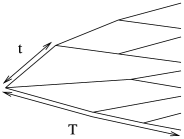
Figure 3: Ultrametric tree with all tips at equal distance $T$ from the root. The root has $k=3$ children here, and $t$ is the minimum distance from the root to its children.

One consequence is that there is no consistent estimator for $\mu$. To illustrate this, we consider the MLE of $\mu$ and provide a lower bound for its variance. We let $t$ be the length of the shortest branch stemming from the root and $k$ the number of daughters of the root (Figure 3).

Theorem 2.2

Assume OU model (1) on an ultrametric tree. Let $\hat{\mu}$ be the MLE of $\mu$ conditional on some possibly wrong value $\alpha_{*}$ of $\alpha$. Then

$$\operatorname{var}(\hat{\mu})\geq\frac{\sigma^{2}}{2\alpha}e^{-2\alpha T}\biggl{(}1+\frac{e^{2\alpha t}-1}{k}\biggr{)}.$$ (7)

The equality holds if and only if $\alpha$ is known ($\alpha_{*}=\alpha$) and the tree is a star tree with the root as unique internal node, in which case $k=n$ and $t=T$. If $T$ is bounded as the sample size $n$ grows and $\alpha>0$, then $\hat{\mu}$ is not consistent.

The second part of the theorem follows directly from the lower bound (7). Note that $\hat{\mu}$ is Gaussian with mean $\mu$. Therefore, the lower bound of its variance implies that $\hat{\mu}$ cannot converge to $\mu$. Hence, it is not consistent.

The assumption that $\alpha>0$ is trivial. When $\alpha=0$, the OU process reduces to a BM where $\mu$ has no influence on the process. In that case, $\mu$ is no longer a parameter in the model. As expected, the lower bound on the variance of $\hat{\mu}$ is heavily influenced by the actual value of the correlation parameter $\alpha$. The precision of $\hat{\mu}$ is weakest when autocorrelation is strong, that is, when $\alpha$ is small, for a given value of $\gamma=\sigma^{2}/(2\alpha)$.

The ultrametric assumption is necessary. If the tree is not ultrametric, model (2) predicts unequal variances and most importantly unequal means at the tips. Such trees can carry more information about $\mu$. Consider, for instance, the star tree in Figure 4, in which all tips are directly connected to the root, by a branch of

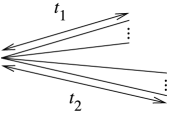
Figure 4: Example of a nonultrametric tree on which $\mu$ can be consistently estimated.

length $t_{1}$ for half of the tips and of length $t_{2}$ for the other half of the tips. If $t_{1}\neq t_{2}$ the variance of $\hat{\mu}$ goes to $0$ as the sample size grows (see Appendix B.2), thus providing a counterexample to Theorem 2.2 when the ultrametric assumption is violated.

Proof of Theorem 2.2 To prove (7), we note that $\hat{\mu}=(\mathbf{1}^{t}V_{\alpha_{*}}^{-1}\mathbf{1})^{-1}\*\mathbf{1}^{t}V_{\alpha_{*}}^{-1}Y$, where $\mathbf{1}$ is a vector of ones. This estimator is unbiased and has variance $\frac{\sigma^{2}}{2\alpha}(\mathbf{1}^{t}V_{\alpha}^{-1}\mathbf{1})^{-1}$ when $\alpha_{*}=\alpha$ is known. Its variance is larger when $\alpha$ is unknown, by the Gauss–Markov theorem. For this reason, we only need to prove the following lemma (which is done in Appendix B.2).

Lemma 2.3

For all $\alpha>0$, $(\mathbf{1}^{t}V_{\alpha}^{-1}\mathbf{1})^{-1}\geq e^{-2\alpha T}+\frac{1}{k}(e^{-2\alpha(T-t)}-e^{-2\alpha T})$ with equality if the tree is a star with $k$ branches stemming from the root.

Theorem 2.2 can be applied to any tree growth asymptotic framework, so long as $T$ is bounded. For instance, both conditions are met almost surely with $k=2$ under the coalescent model [Kingman (1982a, 1982b)]. Even if these conditions do not hold asymptotically, (7) provides a finite-sample upper bound on the estimator’s precision. This inequality can be used, for instance, under the Yule model of tree growth [Yule (1925), Aldous (2001)] if we let both $T$ and $n$ increase indefinitely.

2.4 Microergodicity of the autocorrelation parameter $(\gamma,\alpha)$

Theorem 2.4

Under OU model (1) and condition (C):

Let $t_{0}$ be a limit point of $(T_{i})_{i\in\mathscr{I}}$. Then $f_{t_{0}}(\gamma,\alpha)$ is microergodic, where

$$f_{t}(\gamma,\alpha)=\cases{\gamma\bigl{(}1-e^{-2\alpha t}\bigr{)},&\quad$t>0$,\cr\gamma\alpha,&\quad$t=0$.}$$

If $\sum_{i\in\mathscr{I}}{(T_{i}-t)^{2}}=\infty$ for all $t\geq 0$, then $(\gamma,\alpha)$ is microergodic. Note that this condition is satisfied if $(T_{i})_{i\in\mathscr{I}}$ has 2 or more limit points.

The key idea is to reduce the tree for a lower bound of $r(\mathbb{T}_{n})$. We will consider subtrees that provide independent contrasts, sufficient to ensure microergodicity. Our constructive proof could be used to construct estimators based on a restricted set of contrasts, but we do not pursue this here. Let $i\in\mathscr{I}$ be an arbitrary internal node, and $Y^{i}_{1}$, $Y^{i}_{2}$ be two leaves having $i$ as their most recent common ancestor. Let $p_{i}$ be the path connecting $Y^{i}_{1}$ and $Y^{i}_{2}$. We define $C^{p_{i}}_{i}=Y^{i}_{1}-Y^{i}_{2}$ as a contrast with respect to internal node $i$ and path $p_{i}$. For convenience, we define $T_{C^{p_{i}}_{i}}=T_{i}$. The following lemma is proved in Appendix B.2.

Lemma 2.5

We have that $C^{p_{i}}_{i}\sim N(0,2\gamma(1-e^{-2\alpha T_{i}}))$. Also, $C^{p_{i_{1}}}_{i_{1}}$ and $C^{p_{i_{2}}}_{i_{2}}$ are independent if their paths $p_{i_{1}}$ and $p_{i_{2}}$ do not intersect.

Proof of part 2.4 We denote $\mathscr{I}^{\mathbb{T}}_{S}=\{i\dvtx T_{i}\in S,i\in\mathscr{I}^{\mathbb{T}}\}$ the set of internal nodes of $\mathbb{T}$ whose ages lie in $S$. Let $(\gamma_{1},\alpha_{1})$ and $(\gamma_{2},\alpha_{2})$ such that $f_{t_{0}}(\gamma_{1},\alpha_{1})\neq f_{t_{0}}(\gamma_{2},\alpha_{2})$. Denote

$$g(t)=\frac{1}{2}\biggl{(}\frac{f_{t}(\gamma_{1},\alpha_{1})}{f_{t}(\gamma_{2},\alpha_{2})}+\frac{f_{t}(\gamma_{2},\alpha_{2})}{f_{t}(\gamma_{1},\alpha_{1})}-2\biggr{)},\qquad t\in\bigl{[}0,T^{*}\bigr{]},$$

and let $\delta=g(t_{0})/2>0$. Note that $g$ is continuous at $t_{0}$, so there exists $\varepsilon_{\delta}>0$ such that $g(t)\geq g(t_{0})-\delta$ for all $t$ satisfying $|t-t_{0}|<\varepsilon_{\delta}$. We now use Lemma B.1 (in Appendix B.1) to select a large set ${\mathscr{C}}_{n}$ of independent contrasts with respect to internal nodes whose ages are in $(t_{0}-\varepsilon_{\delta},t_{0}+\varepsilon_{\delta})$ such that $|{\mathscr{C}}_{n}|\geq\frac{1}{2}|\mathscr{I}^{\mathbb{T}_{n}}_{(t_{0}-\varepsilon_{\delta},t_{0}+\varepsilon_{\delta})}|$. Let $r({\mathscr{C}}_{n})$ be the entropy distance between $P_{\theta_{1}}$ and $P_{\theta_{2}}$ on the $\sigma$-algebra generated by ${\mathscr{C}}_{n}$. By (3) and direct calculation,

$$r(\mathbb{T}_{n})\geq r(\mathscr{C}_{n})=\sum_{C\in\mathscr{C}_{n}}g(T_{C})\geq|\mathscr{C}_{n}|\bigl{(}g(t_{0})-\delta\bigr{)}=\delta|\mathscr{C}_{n}|\geq\frac{\delta}{2}\bigl{|}\mathscr{I}^{\mathbb{T}_{n}}_{(t_{0}-\varepsilon_{\delta},t_{0}+\varepsilon_{\delta})}\bigr{|}.$$

Clearly $|\mathscr{I}^{\mathbb{T}_{n}}_{(t_{0}-\varepsilon_{\delta},t_{0}+\varepsilon_{\delta})}|\to\infty$ if $t_{0}$ is a limit point of $(T_{i})_{i\in\mathscr{I}}$. Therefore $f_{t_{0}}(\gamma,\alpha)$ is microergodic.

Proof of part 2.4 First, we consider the case when $(T_{i})_{i\in\mathscr{I}}$ has two different limit points $t_{1}$ and $t_{2}$. By part 2.4, $f_{t_{1}}(\gamma,\alpha)$ and $f_{t_{2}}(\gamma,\alpha)$ are microergodic. So, $(\gamma,\alpha)$ is microergodic by the following lemma (proved in Appendix B.2):

Lemma 2.6

Assume there exists $t_{1}\neq t_{2}$ such that both $f_{t_{1}}(\gamma_{1},\alpha_{1})=f_{t_{1}}(\gamma_{2},\alpha_{2})$ and $f_{t_{2}}(\gamma_{1},\alpha_{1})=f_{t_{2}}(\gamma_{2},\alpha_{2})$. Then $(\gamma_{1},\alpha_{1})=(\gamma_{2},\alpha_{2})$.

We now turn to the case when $(T_{i})_{i\in\mathscr{I}}$ has only one limit point $t_{0}$. We already know that $f_{t_{0}}(\gamma,\alpha)$ is microergodic, so we may assume that $f_{t_{0}}(\gamma_{1},\alpha_{1})=f_{t_{0}}(\gamma_{2},\alpha_{2})$, that is, $g(t_{0})=0$. Denote $\mathscr{I}_{(t_{0},\infty)}=\bigcup^{\infty}_{n=1}{\mathscr{I}^{\mathbb{T}_{n}}_{(t_{0},\infty)}}$ and $\mathscr{I}_{[0,t_{0}]}=\bigcup^{\infty}_{n=1}{\mathscr{I}^{\mathbb{T}_{n}}_{[0,t_{0}]}}$. The condition in 2.4 implies that $\sum_{i\in\mathscr{I}_{(t_{0},\infty)}}(T_{i}-t_{0})^{2}=\infty$ or $\sum_{i\in\mathscr{I}_{[0,t_{0}]}}(T_{i}-t_{0})^{2}=\infty$ or both. We now use Lemma B.2 (Appendix B.1) to select, for each $n$, a large set $\mathscr{C}_{n}$ of independent contrasts such that $\lim_{n}\sum_{C\in\mathscr{C}_{n}}{(T_{C}-t_{0})^{2}}=\infty$. Again, by (3) we have $r(\mathbb{T}_{n})\geq r(\mathscr{C}_{n})=\sum_{C\in\mathscr{C}_{n}}g(T_{C})$, which we approximate below. If $t_{0}=0$, by Taylor expansion there exists $c(\alpha,T^{*})$ such that $|e^{-2\alpha x}-1+2\alpha x-2\alpha^{2}x^{2}+\frac{4}{3}\alpha^{3}x^{3}|\leq c(\alpha,T^{*})x^{4}$ for every $x$ satisfying $|x|<T^{*}$. Similarly, if $t_{0}>0$ there exists $c(\alpha,T^{*})$ such that $|e^{-2\alpha x}-1+2\alpha e^{-2\alpha t_{0}}(x-t_{0})-2\alpha^{2}e^{-2\alpha t_{0}}(x-t_{0})^{2}|\leq c(\alpha,T^{*})x^{3}$ for every $x$ satisfying $|x-t_{0}|<T^{*}$. In both cases, we can then write

$$r(\mathscr{C}_{n})=\frac{1}{2}\sum_{C\in\mathscr{C}_{n}}{\bigl{(}h_{t_{0}}(\alpha_{1})-h_{t_{0}}(\alpha_{2})\bigr{)}}^{2}(T_{C}-t_{0})^{2}+o(T_{C}-t_{0})^{2},$$

where $o(T_{C}-t_{0})^{2}$ is uniform in $n$, $h_{0}(\alpha)=\alpha$ and $h_{t}(\alpha)=2\alpha e^{-2\alpha t}/(1-e^{-2\alpha t})$ for $t>0$. Therefore $r(\mathscr{C}_{n})\to\infty$ unless $(\gamma_{1},\alpha_{1})=(\gamma_{2},\alpha_{2})$. Hence $(\gamma,\alpha)$ is microergodic.

Theorem 2.4 part 2.4 gives a very general sufficient condition ensuring the microergodicity of $(\gamma,\alpha)$. Unfortunately, it is not a necessary condition in general. To prove so, we consider the particular case when $\mathbb{T}_{n}$ is a symmetric tree, that is, a tree in which each internal node is the parent of subtrees of identical shapes (see Figure 5). We give below 3 examples in which

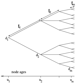
Figure 5: Symmetric trees with $m=4$ levels.

$(T_{i})_{i\in\mathscr{I}}$ has only one limit point $t_{0}$, and the condition in Theorem 2.4 part 2.4 is violated. Two examples illustrate the nonmicroergodicity of $(\gamma,\alpha)$, one in which $t_{0}>0$ and one in which $t_{0}=0$. In the last example the condition in 2.4 is violated, yet $(\gamma,\alpha)$ is microergodic.

Theorem 2.7

Consider the OU model (1) on symmetric trees with $m$ levels and whose internal nodes at level $i$ have $d_{i}$ descendants along branches of length $t_{i}$.

1. Increasing node degrees. Consider a nested sequence of symmetric trees with a fixed number of levels $m$ and fixed branch lengths $t_{1},t_{2},\ldots,t_{m}$. Assume that the number of descendants $d_{m}$ at the last level goes to infinity, but all other $d_{1},\ldots,d_{m-1}$ are fixed, so that $t_{m}>0$ is the only limit point of $(T_{i})_{i\in\mathscr{I}}$. Then $(\gamma,\alpha)$ is not microergodic.

2. Dense sampling near the tips, or at distance $t_{0}$ from the tips. Consider a nested sequence of symmetric trees with a growing number of levels $m$, $d_{k}=d$ descendants at all levels $k\geq 1$ and such that the age of nodes at level $k$ is $u_{k}=q^{k}+t_{0}$ for some $0<q<1$. Suppose that $dq^{2}<1$, to guarantee the violation of the condition in Theorem 2.42.4:

   1. [(ii)]

   2. If $t_{0}=0$, then $(\gamma,\alpha)$ is not microergodic.

   3. If $t_{0}>0$, then $(\gamma,\alpha)$ is microergodic.

We discuss here the key ingredients of the proof. The technical details are provided in Appendix B.2. Note that node ages are counted with multiplicity. Here $u_{i}$ is the age of the $d_{1}\cdots d_{i-1}$ internal nodes at level $i$, with multiplicity $d_{i}-1$ for each. Hence in part (a) $u_{m}=t_{m}$ is the only limit point. For a symmetric tree, the eigenvalues of the covariance matrix are $\gamma\lambda_{k}(\alpha)$ with multiplicity $d_{1}\cdots d_{k-1}(d_{k}-1)$, where $\lambda_{k}(\alpha)=\sum_{i=k}^{m}d_{i+1}\cdots d_{m}(e^{-2\alpha u_{i+1}}-e^{-2\alpha u_{i}})$ (Appendix A). In (a), only the multiplicity of the smallest eigenvalue increases to infinity when the tree grows. If $(\gamma_{1},\alpha_{1})$ and $(\gamma_{2},\alpha_{2})$ share the same smallest eigenvalue, that is, if $\gamma_{1}\lambda_{m}(\alpha_{1})=\gamma_{2}\lambda_{m}(\alpha_{2})$, then insufficient information is gained to distinguish between $P_{(\gamma_{1},\alpha_{1})}$ and $P_{(\gamma_{2},\alpha_{2})}$ when the tree grows. In (b), the eigenvalue with the largest multiplicity is also the smallest, $\gamma\lambda_{m}(\alpha)=\gamma(1-e^{-2\alpha u_{m}})$. It converges to $0$ when $t_{0}=0$ and to $\gamma(1-e^{-2\alpha t_{0}})>0$ when $t_{0}>0$, yielding too little information in (i) when $t_{0}=0$, but more information to distinguish between $P_{(\gamma_{1},\alpha_{1})}$ and $P_{(\gamma_{2},\alpha_{2})}$ in (ii) when $t_{0}>0$.

3 Different convergence rates of ML estimators for different microergodic parameters

Section 2 suggests that the different parameters may not be estimated at the same rate. Indeed, if $t_{0}$ is the only limit point of internal node ages, then Theorem 2.4 shows that $f_{t_{0}}(\gamma,\alpha)$ is microergodic regardless of whether condition in 2.4 is satisfied or not. Therefore, the ML or REML estimate of $f_{t_{0}}(\gamma,\alpha)$ is expected to converge to the true value at a faster rate than the estimate of other parameters. In particular, for $t_{0}=0$ the ML estimate of $\sigma^{2}$ is expected to converge at a faster rate than that of $\alpha$, which might not even be consistent. Here we identify cases with unequal convergence rates both theoretically and empirically.

3.1 Faster convergence of the REML estimator for $f_{t_{0}}(\gamma,\alpha)$ than for $\alpha$ and $\gamma$

We focus here on the symmetric tree growth model from Theorem 2.7 part (a) with nodes of increasing degrees, but we consider here the case when $\tilde{n}=n/d_{m}=d_{1}\cdots d_{m-1}$ increases indefinitely to ensure the microergodicity of $\gamma$ and $\alpha$. We show that the REML estimator of $(\gamma,\alpha)$ is consistent and asymptotic normally distributed. We further show that $f_{t_{m}}(\gamma,\alpha)$, which is microergodic regardless of the growth of $\tilde{n}$, is estimated at a faster rate than $\alpha$ or $\gamma$, which have stronger requirements to be microergodic.

Theorem 3.1

Consider the asymptotic growth model from above with OU model (1). Denote $\nu=\gamma(1-e^{-2\alpha t_{m}})$. Then the REML estimator $(\hat{\nu},\hat{\alpha})$ is consistent and

$$\pmatrix{\sqrt{n}(\hat{\nu}-\nu)\cr\sqrt{\tilde{n}}(\hat{\alpha}-\alpha)}\stackrel{{\scriptstyle d}}{{\rightarrow}}N\left(\mathbf{0},\pmatrix{8\nu^{2}&0\cr 0&v_{\alpha}}\right).$$

Moreover, if $n/\tilde{n}=d_{m}$ converges to infinity, then $\sqrt{\tilde{n}}(\hat{\gamma}-\gamma,\hat{\alpha}-\alpha)^{t}$ converges to a centered normal distribution and the asymptotic correlation between $\log\hat{\gamma}$ and $\log(1-e^{-2\hat{\alpha}t_{m}})$ is $-1$.

The proof in Appendix B.3 gives the expression for $v_{\alpha}$. With increasing node degrees at $m$ levels, the age of nodes at the last level $t_{m}$ is the only limit point of $(T_{i})_{i\in\mathscr{I}}$ if $\tilde{n}$ is bounded. The growth of $\tilde{n}$ ensures at least 2 limit points and the consistency of all parameters. Our results show that the rate of convergence is $\tilde{n}^{-1/2}$ for both $\hat{\alpha}$ and $\hat{\gamma}$. However, only one limit point ($t_{m}$) is required for the consistent estimation of $\nu=f_{t_{m}}(\gamma,\alpha)$, which is microergodic regardless of $\tilde{n}$. Accordingly, the convergence rate of $\hat{\nu}$ is $n^{-1/2}$, which can be much faster than $\tilde{n}^{-1/2}$.

3.2 Simulations on a very large real tree

In this section we use simulations to investigate the properties of the MLE of the OU parameters on a real tree, comprising 4507 mammal species from Bininda-Emonds et al. (2007).

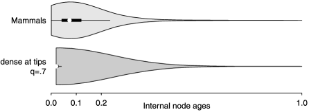
Figure 6: Distribution of node ages in the mammal tree (top) and in a symmetric tree (bottom) of similar size $n=2^{12}=4096$ with $d=2$ at each level, levels being added near the tips at ages $q^{m}$. The value $q=0.7\approx 2^{-1/2}$ is the largest at which $\alpha$ and $\gamma$ are not microergodic.

Figure 6 shows the distribution of node ages for this tree, and for a symmetric tree with dense sampling near the tips described in Theorem 2.7(b), on which $\alpha$ and $\gamma$ are not microergodic. Both distributions show a high density of very young nodes. Under the symmetric tree asymptotics with $0$ as the only limit point, $\sigma^{2}$ is microergodic while $(\gamma,\alpha)$ might not be. Note that this is also the behavior under spatial infill asymptotics in dimension $d\leq 3$. For real trees like this mammal tree, therefore, we expect the MLE of $\sigma^{2}$ to converge quickly, and the MLE of $\alpha$ to converge more slowly or not at all.

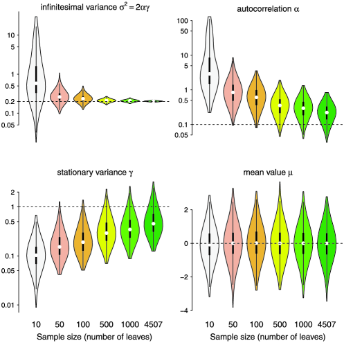
Figure 7: Violin plots showing the distribution of the MLE of $\mu$, $\gamma$, $\alpha$ and $\sigma^{2}=2\gamma\alpha$ on trees subsampled from the mammal phylogeny in Bininda-Emonds et al. (2007) with 2000 simulations at each sample size. The true values were $\mu=0$, $\gamma=1$, $\alpha=0.1$ and $\sigma^{2}=0.2$.

For various sample sizes from 10 to 4507 (full tree), we simulated data from the OU model with $\mu=0$, $\gamma=1$ and $\alpha=0.1$, so $\sigma^{2}=0.2$. We created 20 sequences of six nested trees from 4507 to 10 leaves by randomly selecting subsets of leaves, conditional on the root being the only common ancestor of the selected leaves to guarantee that all trees have the same height. Trees were all rescaled by the same factor to have height 1. For each tree, we simulated 100 data sets and computed the MLEs $\hat{\mu}$, $\hat{\gamma}$ and $\hat{\alpha}$. As expected, these simulations show that $\hat{\sigma}^{2}$ converges quickly to the true value while $\hat{\alpha}$ and $\hat{\gamma}$ do not (Figure 7). A strong bias is apparent for $\hat{\gamma}$ and $\hat{\alpha}$ even at the largest sample size (4507). Moreover, the correlation between $\log\hat{\alpha}$ and $\log\hat{\gamma}$ converges very fast to $-1$ (Table 1). Also, the lower bound for the variance of $\hat{\mu}$ is very close to the true variance (Table 1). Therefore, this lower bound can be useful in practice at finite sample sizes.

4 Discussion

We considered an Ornstein–Uhlenbeck model of hierarchical autocorrelation and showed that the location parameter, here the mean $\mu$, is not microergodic. We provided the lower bound for the variance of its ML estimator. In practice, these results could have important implications when scientists use OU hierarchical autocorrelation to detect a location shift, that is, a change in $\mu$ along a branch of the tree [e.g., Butler and King (2004), Lavin et al. (2008), Monteiro and Nogueira (2011)]. Often times, the OU model is used with multiple adaptive optima whose placements on the tree are not fully known. Our results suggest that the power to detect such shifts may be low and mostly influenced by the effect size rather than by the sample size. An open question is whether the location of such shifts on the tree can be identified consistently with a growing number of tips.

Table 1: Correlation between $\log\hat{\alpha}$ and $\log\hat{\gamma}$ and variance of $\hat{\mu}$ from simulations. Last line: value of theoretical bound (7) for $\operatorname{var}(\hat{\mu})$, averaged over 20 simulation subtrees

Sample size	10	50	100	500	1000	4507
$\operatorname{cor}(\log\hat{\alpha},\log\hat{\gamma})$	$-0.44$	$-0.927$	$-0.9674$	$-0.9938$	$-0.9971$	$-0.9993$
$\operatorname{var}(\hat{\mu})$	$0.9007$	$0.8455$	$0.8499$	$0.8853$	$0.8789$	$0.8851$
Lower bound (7)	$0.8517$	$0.8472$	$0.8469$	$0.8468$	$0.8468$	$0.8468$

We provide a general sufficient condition for the covariance parameters to be microergodic. Properties of infill asymptotics were recovered when 0 is the only limit point of internal node ages, that is, when new nodes were added closer and closer to already existing tips. In this case, $\sigma^{2}$ is necessarily microergodic. This asymptotics can be appropriate for coalescent trees or when many species diverged recently from a moderate number of genera. We assume here the idealized situation with no error in the tree structure (topology and branch lengths) and no data measurement error, leaving this for future work. With measurement error, the covariance matrix becomes $\gamma\mathbf{V}_{\alpha}+\sigma^{2}_{e}\mathbf{I}$. The error variance $\sigma^{2}_{e}$ is called a nugget effect in spatial statistics. Measurement error with tree-structured correlation is rarely accounted for in applications; but see Ives, Midford and Garland (2007).

For a general tree growth model, by using independent contrasts we can construct a consistent estimator for $f_{t_{0}}(\gamma,\alpha)$ where $t_{0}$ is any limit point of $(T_{i})_{i\in\mathscr{I}}$. If $(T_{i})_{i\in\mathscr{I}}$ has at least two limit points, then by Lemma 2.6, we can construct a consistent estimator for $(\gamma,\alpha)$. This proposed estimator is based on a restricted set of well-chosen contrasts, but it uses fewer contrasts and thus less information than the conventional REML estimator. We conjecture that if $(\gamma,\alpha)$ is microergodic, the REML estimator of $(\gamma,\alpha)$ is also consistent and asymptotically normal.

The microergodicity results suggest that parameters may not all be estimated at the same rate. Indeed, we show that the REML of $\alpha$ converges at a slower rate than $n^{-1/2}$ under a symmetric tree asymptotic framework. Similarly, our simulations suggest that the mammalian tree with 4507 species shares features similar to those under infill asymptotics (in low dimension) and under dense sampling near the tips of symmetric trees, where $\sigma^{2}$ can be consistently estimated but $\alpha$ and $\gamma$ cannot. On the real tree, the MLE of $\sigma^{2}$ converges quickly to the true value while that of $\alpha$ and $\gamma$ do not. This behavior may explain a lack of power to discriminate between a model of neutral evolution ($\alpha=0$) versus a model with natural selection ($\alpha\neq 0$), as observed in Cooper and Purvis (2010). It would be interesting to know if most real trees share the “dense tip” asymptotic behavior, or how frequently a “dense root” asymptotic is applicable instead. Our results point to the distribution on node ages as indicative of the most appropriate asymptotic regime.

Appendix A Spectral decomposition of the OU covariance matrix on symmetric trees

We consider here symmetric trees (Figure 5) with $m$ levels of internal nodes, the root being at level $1$. Each node at level $k$ is connected to $d_{k}\geq 2$ children by branches of length $t_{k}$. The age of nodes at level $k$ is then $u_{k}=t_{k}+\cdots+t_{m}$. Under the OU model (1), the correlation matrix $\mathbf{V}_{\alpha}$ is identical to that obtained under a BM model along a tree with an extra branch extending from the root and with transformed branch lengths $\mathbf{t}^{\mathrm{BM}}$,

$$t^{\mathrm{BM}}_{k}(\alpha)=\cases{1-e^{-2\alpha t_{m}},&\quad for $k=m$,\cr e^{-2\alpha u_{k+1}}-e^{-2\alpha u_{k}},&\quad$1\leq k\leq m-1$,\cr e^{-2\alpha u_{1}},&\quad$k=0$ (extra root branch).}$$

Therefore, we can derive the eigen-decomposition of $\mathbf{V}_{\alpha}(\mathbf{t})=\mathbf{V}^{\mathrm{BM}}_{\alpha}(\mathbf{t}^{\mathrm{BM}})$ as done in Ané (2008). The eigenvalues, from greatest to smallest, are

$$\lambda_{k}=n\sum_{i=k}^{m}{\frac{t^{\mathrm{BM}}_{i}(\alpha)}{d_{1}\cdots d_{i}}}=\sum_{i=k}^{m}d_{i+1}\cdots d_{m}\bigl{(}e^{-2\alpha u_{i+1}}-e^{-2\alpha u_{i}}\bigr{)}$$

with multiplicity $d_{1}\cdots d_{k-1}(d_{k}-1)$, for $k=0,\ldots,m$ and $u_{m+1}$ set to $0$ and $u_{0}$ to $\infty$. Furthermore, Ané (2008) showed that the eigenvectors of $\mathbf{V}^{\mathrm{BM}}_{\alpha}$ are independent of the tree’s branch lengths, which implies here that the eigenvectors of $\mathbf{V}_{\alpha}$ are independent of $\alpha$. Each eigenvector corresponding to $\lambda_{k}(\alpha)$ represents a contrast between the descendants of a node at level $k$. One exception is the eigenvector associated with the extra root branch and largest eigenvalue $\lambda_{0}$. This eigenvector is $\mathbf{1}$ and has multiplicity $1$.

Appendix B Supporting lemmas and technical proofs

B.1 Procedures for choosing independent contrasts

Lemma B.1

Let $\mathbb{T}$ be an ultrametric tree. For every $a<b$, we can choose a set of independent contrasts $\mathscr{C}$ with respect to some of the internal nodes in $\mathscr{I}^{\mathbb{T}}_{(a,b)}$ such that $|\mathscr{C}|\geq\frac{1}{2}|\mathscr{I}^{\mathbb{T}}_{(a,b)}|$.

We choose contrasts as follows, starting with $\mathscr{C}=\varnothing$ and $\mathbb{T}_{0}=\mathbb{T}$. At step $n$, we choose an internal node $i_{n}\in\mathscr{I}^{\mathbb{T}_{n-1}}_{(a,b)}$ of minimum age, and a path $p_{i_{n}}$ connecting any two tips having $i_{n}$ as their common ancestor. We update $\mathscr{C}=\mathscr{C}\cup\{C^{p_{i_{n}}}_{i_{n}}\}$ and obtain tree $\mathbb{T}_{n}$ from $\mathbb{T}_{n-1}$ by dropping all descendants of $i_{n}$. We stop when $\mathscr{I}^{\mathbb{T}_{n}}_{(a,b)}=\varnothing$. The procedure guarantees that the paths do not intersect, hence the contrasts are independent. Furthermore, $\mathscr{I}^{\mathbb{T}_{n}}_{(a,b)}=\mathscr{I}^{\mathbb{T}_{n-1}}_{(a,b)}\setminus\{i_{n},i^{\prime}_{n}\}$ where $i^{\prime}_{n}$ is the parent of $i_{n}$, so $|\mathscr{C}|\geq|\mathscr{I}^{\mathbb{T}}_{(a,b)}|/2$.

Lemma B.2

Let $\mathbb{T}$ be an ultrametric tree of height $T$. For all $t\in[0,T]$: [(a)]

There exists a set of independent contrasts $\mathscr{C}$ with respect to nodes in $\mathscr{I}^{\mathbb{T}}_{[0,t]}$ such that $\sum_{C\in\mathscr{C}}{(T_{C}-t)^{2}}\geq\frac{1}{2}\sum_{i\in\mathscr{I}^{\mathbb{T}}_{[0,t]}}{(T_{i}-t)^{2}}$.

There exists a set of independent contrasts $\mathscr{C}$ with respect to nodes in $\mathscr{I}^{\mathbb{T}}_{(t,\infty)}$ such that $\sum_{C\in\mathscr{C}}{(T_{C}-t)^{2}}\geq\frac{1}{4}[(T-t)^{2}+\sum_{i\in\mathscr{I}^{\mathbb{T}}_{(t,\infty)}}{(T_{i}-t)^{2}}].$

Proof of Lemma B.2.  (a) The procedure in the proof of Lemma B.1 gives us a desired set of contrasts. Indeed, let $(i_{k})_{k=1}^{m}$ be the chosen set of nodes and $(i^{\prime}_{k})_{k=1}^{m}$ be their parents. Then $\mathscr{I}^{\mathbb{T}}_{[0,t]}\subset\bigcup_{k=1}^{m}\{i_{k},i^{\prime}_{k}\}$, hence

$$\sum_{i\in\mathscr{I}^{\mathbb{T}}_{[0,t]}}(T_{i}-t)^{2}\leq\sum_{k=1}^{m}(T_{i_{k}}-t)^{2}+(T_{i^{\prime}_{k}}-t)^{2}\leq 2\sum_{k=1}^{m}(T_{i_{k}}-t)^{2}=2\sum_{C\in\mathscr{C}}(T_{C}-t)^{2}.$$

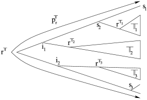
Figure 8: Recursive construction of independent contrasts, taken with respect to the root at each step.

(b) Contrasts are chosen by induction, starting with $\mathscr{C}=\varnothing$. Let $r^{\mathbb{T}}$ be the root of $\mathbb{T}$. If $r^{\mathbb{T}}\notin\mathscr{I}^{\mathbb{T}}_{(t,T]}$, then we stop; else we update $\mathscr{C}=\mathscr{C}\cup\{C^{p_{r}^{\mathbb{T}}}_{r^{\mathbb{T}}}\}$ where the path $p_{r}^{\mathbb{T}}$ is chosen carefully as follows. From each child of the root, the path descends toward the tips. Each time an internal node is encountered, a decision needs to be made to either go left or right. Of the two children of the internal node, the path is connected to the youngest (Figure 8). We then remove from $\mathbb{T}$ the path $p_{r}^{\mathbb{T}}$ and the edges connected to it. What is left is a forest, a set of subtrees of $\mathbb{T}$, one which we repeat the procedure, recursively extracting one path and its corresponding contrast from each subtree.

We now prove by induction that this procedure gives us a desired set of contrasts. This is easy to see for $\leq 3$ tips. Assume that it is true for every tree with $\leq$$m$ tips, and that $\mathbb{T}$ has $m+1$ tips. Let $i_{1}$ and $i_{2}$ be the two children of $r^{\mathbb{T}}$. Let $(\mathbb{T}_{k})_{k=1}^{l}$ be the subtrees obtained after removing $p_{r}^{\mathbb{T}}$ and the edges connected to it, and such that $r^{\mathbb{T}_{k}}\in\mathscr{I}^{\mathbb{T}}_{(t,T]}$. Let $s_{k}$ be the sibling of $r^{\mathbb{T}_{k}}$ in $\mathbb{T}$ ($s_{k}$ could be a leaf). By construction, $T_{s_{k}}\leq T_{r^{\mathbb{T}_{k}}}$. Let $\mathscr{C}_{k}$ be the set of contrasts obtained from $\mathbb{T}_{k}$. We have $\mathscr{I}^{\mathbb{T}}_{(t,T]}\subset\{r^{\mathbb{T}},i_{1},i_{2}\}\bigcup_{k=1}^{l}\mathscr{I}^{\mathbb{T}_{k}}_{(t,T]}\cup\{s_{k}\}$ and $\mathscr{C}=\{r^{\mathbb{T}}\}\bigcup_{k=1}^{l}\mathscr{C}_{k}$. Therefore,

$$4\sum_{C\in\mathscr{C}}{(T_{C}-t)^{2}} = 4(T_{r^{\mathbb{T}}}-t)^{2}+4\sum_{k=1}^{l}{\sum_{C\in\mathscr{C}_{k}}{(T_{C}-t)^{2}}}$$

$$\geq 2(T_{r^{\mathbb{T}}}-t)^{2}+\bigl{(}\max\{T_{i_{1}},t\}-t\bigr{)}^{2}+\bigl{(}\max\{T_{i_{2}},t\}-t\bigr{)}^{2}$$

$${}+\sum_{k=1}^{l}\biggl{\{}(T_{r^{\mathbb{T}_{k}}}-t)^{2}+\sum_{i\in\mathscr{I}^{\mathbb{T}_{k}}_{(t,T]}}{(T_{i}-t)^{2}}\biggr{\}}$$

$$\geq (T_{r^{\mathbb{T}}}-t)^{2}+\sum_{i\in\mathscr{I}^{\mathbb{T}}_{(t,T]}}{(T_{i}-t)^{2}}.$$

B.2 Technical proofs for Section 2

Counter example for Theorem 2.2 on nonultrametric trees

Let $a=e^{-\alpha t_{1}}$ and $b=e^{-\alpha t_{2}}$. It is easy to see that $\mathbf{V}_{\alpha}$ can be expressed in terms of the $n/2\times n/2$ identity matrix $\mathbf{I}$ as $\mathbf{V}_{\alpha}=\operatorname{diag}((1-a^{2})\mathbf{I},(1-b^{2})\mathbf{I})+(a\mathbf{1}^{t},b\mathbf{1}^{t})^{t}(a\mathbf{1}^{t},b\mathbf{1}^{t})$. We then get $\mathbf{V}_{\alpha}^{-1}$ using Woodbury’s formula, then $\mathbf{1}^{t}\mathbf{V}^{-1}_{\alpha}\mathbf{1}=n(\frac{1}{1-a^{2}}+\frac{1}{1-b^{2}}+\frac{n(a-b)^{2}}{(1-a^{2})(1-b^{2})})/(1+\frac{na^{2}}{1-a^{2}}+\frac{nb^{2}}{1-b^{2}}).$ If $t_{1}\neq t_{2}$, then $a\neq b$ and $\operatorname{var}(\hat{\mu})=(\mathbf{1}^{t}V^{-1}_{\alpha}\mathbf{1})^{-1}$ goes to 0 as claimed.

Proof of Lemma 2.3.  We will first prove $\mathbf{V}_{\alpha}\geq e^{-2\alpha T}\mathbf{J}_{n}$ by induction on the number of tips, where $\mathbf{J}_{n}=\mathbf{1}\mathbf{1}^{t}$. Clearly, this is true for trees with a single tip. Now consider a tree with $n$ tips, and consider its $k$ subtrees obtained by removing the $k$ branches stemming from the root. Let $T_{1},\ldots,T_{k}$ be the heights of these subtrees, that is, the age of their roots. Their number of tips $n_{1},\ldots,n_{k}$ is at most $n-1$. So by induction, the covariance matrices $\mathbf{V}^{(1)}_{\alpha},\ldots,\mathbf{V}^{(k)}_{\alpha}$ associated with these subtrees must satisfy $\mathbf{V}^{(i)}_{\alpha}\geq e^{-2\alpha T_{i}}\mathbf{J}_{n_{i}}$. Therefore $\mathbf{V}_{\alpha}-e^{-2\alpha T}\mathbf{J}_{n}\geq\operatorname{diag}(\mathbf{V}^{(i)}_{\alpha}-e^{-2\alpha T_{i}}\mathbf{J}_{n_{i}})\geq 0$ is true for all trees. Now we use the definition of $t$ and go a step further using that $\mathbf{V}^{(i)}_{\alpha}-e^{-2\alpha T}\mathbf{J}_{n_{i}}\geq(e^{-2\alpha T_{i}}-e^{-2\alpha T})\mathbf{J}_{n_{i}}\geq(e^{-2\alpha(T-t)}-e^{-2\alpha T})\mathbf{J}_{n_{i}}$ for all $i=1,\ldots,k$. This implies that $\mathbf{V}_{\alpha}-e^{-2\alpha T}\mathbf{J}_{n}\geq(e^{-2\alpha(T-t)}-e^{-2\alpha T})\operatorname{diag}(\mathbf{J}_{n_{1}},\ldots,\mathbf{J}_{n_{k}})\geq\frac{1}{k}(e^{-2\alpha(T-t)}-e^{-2\alpha T})\mathbf{J}_{n},$ from which Lemma 2.3 follows easily.

Proof of upper bound (6).  Assume here that $\alpha_{1}=\alpha_{2}$ and $\gamma_{1}=\gamma_{2}=\gamma$. Since $(Y_{i})_{i=1}^{n}$ have the same covariance matrix $\gamma{\mathbf{V}}$ under both distributions $P_{\theta_{1}}$ and $P_{\theta_{2}}$, it is easy to see that $r(\mathbb{T})=(\mu_{1}-\mu_{2})^{2}\mathbf{1}^{t}{\mathbf{V}}^{-1}\mathbf{1}/\gamma$ [Hershey and Olsen (2007)]. The bound $r(\mathbb{T})\leq(\mu_{1}-\mu_{2})^{2}/(\gamma e^{-2\alpha T})$, where $T$ is the age of the root, then follows from Lemma 2.3.

Proof of Lemma 2.5.  First, $\operatorname{var}(C^{p_{i}}_{i})=\operatorname{var}(Y_{1}^{i})+\operatorname{var}(Y_{2}^{i})-2\operatorname{cov}(Y_{1}^{i},Y_{2}^{i})=2\gamma-2\gamma e^{-2\alpha T_{i}}$. Second, consider two paths $p_{i_{1}}$ and $p_{i_{2}}$ that do not intersect. Then, the most recent common ancestor of $Y_{j}^{i_{1}}$ and $Y_{k}^{i_{2}}$ ($j,k\in\{1,2\}$) is the most recent common ancestor of internal nodes $i_{1}$ and $i_{2}$. Therefore, the distance from $Y_{1}^{i_{1}}$ to $Y_{1}^{i_{2}}$ equals the distance from $Y_{2}^{i_{1}}$ to $Y_{1}^{i_{2}}$. Hence $\operatorname{cov}(Y_{1}^{i_{1}},Y_{1}^{i_{2}})=\operatorname{cov}(Y_{2}^{i_{1}},Y_{1}^{i_{2}})$. Similarly, $\operatorname{cov}(Y_{1}^{i_{1}},Y_{2}^{i_{2}})=\operatorname{cov}(Y_{2}^{i_{1}},Y_{2}^{i_{2}})$. Therefore $\operatorname{cov}(C^{p_{i}}_{i_{1}},C^{p_{i}}_{i_{2}})=\operatorname{cov}(Y_{1}^{i_{1}}-Y_{2}^{i_{1}},Y_{1}^{i_{2}}-Y_{2}^{i_{2}})=0$.

Proof of Lemma 2.6.  Define $h_{1}(x)=(1-e^{-2x\alpha_{2}})/(1-e^{-2x\alpha_{1}})$, and assume $t_{1}\neq 0$ and $t_{2}\neq 0$. From the system of equations, we have $\gamma_{1}/\gamma_{2}=h_{1}(t_{1})=h_{1}(t_{2})$. Now $(\log h_{1})^{\prime}(x)/x=h_{2}(x\alpha_{2})-h_{2}(x\alpha_{1})$ where $h_{2}(x)=\break xe^{-x}/(1-e^{-x})$ is monotone on $(0,\infty)$. So $\alpha_{1}=\alpha_{2}$, and $\gamma_{1}=\gamma_{2}$. If $t_{2}=0$, we make a similar argument because $h_{3}(x)=x/(1-e^{-2xt_{2}})$ is monotone on $(0,\infty)$.

Proof of Theorem 2.7 part (a).  Under the symmetric tree growth model,

$$r(\mathbb{T})=\frac{1}{2}\sum_{k=1}^{m}{d_{1}\cdots d_{k-1}(d_{k}-1)\biggl{(}\frac{\gamma_{2}\lambda_{k}(\alpha_{2})}{\gamma_{1}\lambda_{k}(\alpha_{1})}+\frac{\gamma_{1}\lambda_{k}(\alpha_{1})}{\gamma_{2}\lambda_{k}(\alpha_{2})}-2\biggr{)}}+\biggl{(}m_{1,n}^{2}+\frac{m_{1,n}^{2}}{\sigma_{1,n}^{2}}\biggr{)}.$$

To show this, we consider $\mathbf{h}=(Y_{j,n})_{j\leq n}=\gamma_{1}^{-1/2}\bolds{\Lambda}^{-1/2}(\alpha_{1})\mathbf{P}^{-1}(\mathbf{Y}-\mu_{1}\mathbf{1})$, where $\bolds{\Lambda}(\alpha)=\operatorname{diag}(\lambda_{k}(\alpha))$ contains the eigenvalues $\lambda_{k}$ with their multiplicities, and $\mathbf{P}$ contains the eigenvectors of $\mathbf{V}_{\alpha}$, which do not depend of $\alpha$ (Appendix A). Then $\mathbf{h}$ is orthonormal under $P_{\theta_{1}}$, and orthogonal under $P_{\theta_{2}}$ with variances $(\gamma_{2}/\gamma_{1})\lambda_{k}(\alpha_{2})/\lambda_{k}(\alpha_{1})$ with multiplicities $d_{1}\cdots d_{k-1}(d_{k}-1)$. Furthermore, $E_{2}\mathbf{h}=(\mu_{2}-\mu_{1})\gamma_{1}^{-1/2}\bolds{\Lambda}^{-1/2}(\alpha_{1})\mathbf{P}^{-1}\mathbf{1}$ so that $m_{j,n}=0$ if $j\geq 2$ and $m_{1,n}=(\mu_{2}-\mu_{1})/\sqrt{n\gamma_{1}\lambda_{0}(\alpha_{1})}$, from which $r(\mathbb{T})$ follows.

With increasing node degrees at $m$ levels, it is easy to see that the ratio $\lambda_{k}(\alpha_{1})/\lambda_{k}(\alpha_{2})$ converges to a positive limit for all $k\leq m$. Under the assumption that $d_{k}$ is fixed for $k<m$, the multiplicity of $\lambda_{k}(\alpha)$ is constant as $n$ grows, except for $k=m$. $r(\mathbb{T}_{m})$ is then expressed as a finite sum where all terms are convergent except for the last term ($k=m$) associated with the smallest eigenvalue $\lambda_{m}=1-e^{-2\alpha t_{m}}$. This term is bounded if and only if $\gamma_{1}(1-e^{-2\alpha_{1}t_{m}})=\gamma_{2}(1-e^{-2\alpha_{2}t_{m}})$, in which case $r(\mathbb{T}_{n})$ converges to a finite value. Otherwise, $r(\mathbb{T}_{n})$ goes to infinity. Hence $P_{\theta_{1}}$ and $P_{\theta_{2}}$ are equivalent if and only if $\gamma_{1}(1-e^{-2\alpha_{1}t_{m}})=\gamma_{2}(1-e^{-2\alpha_{2}t_{m}})$, which completes the proof.

Proof of Theorem 2.7 part (b).  We denote here $\lambda_{k}=\lambda_{k,m}$ to emphasize the dependence of $m$. We first consider case (i) when $t_{0}=0$. When $d_{k}=d$ and $u_{k}=q^{k}$, the eigenvalues simplify to

$$\frac{\lambda_{k,m}(\alpha)}{d^{m-k}}=\sum_{j=0}^{m-k-1}\frac{e^{-2\alpha q^{k+1+j}}-e^{-2\alpha q^{k+j}}}{d^{j}}+\frac{1-e^{-2\alpha q^{m}}}{d^{m-k}}.$$ (8)

It is then easy to see that for all $\alpha\geq 0$ and $k$, $\lambda_{k,m}(\alpha)/d^{m-k}$ converges to some finite function of $\alpha$ and $k$. To prove the convergence of $r(\mathbb{T}_{m})$ we will need the following lemma, which is proved later.

Lemma B.3

Let $\gamma_{1}\alpha_{1}=\gamma_{2}\alpha_{2}$, that is, $\sigma_{1}^{2}=\sigma_{2}^{2}$. Then there exists $K$, $c$ and $C$ which depend only on $\alpha_{1},\alpha_{2},d$ and $q$ such that for all $m>k\geq K$,

$$cq^{2k}\leq\frac{\gamma_{2}\lambda_{k,m}(\alpha_{2})}{\gamma_{1}\lambda_{k,m}(\alpha_{1})}+\frac{\gamma_{1}\lambda_{k,m}(\alpha_{1})}{\gamma_{2}\lambda_{k,m}(\alpha_{2})}-2\leq Cq^{2k}.$$

Because $\gamma\alpha$ is microergodic [Theorem 2.4 part 2.4], we can assume $\gamma_{1}\alpha_{1}=\gamma_{2}\alpha_{2}$. Lemma B.3 implies that the first sum in the expression of $r(\mathbb{T}_{m})$ [from the proof of part (a)] is bounded above and below by $\sum_{k=K}^{m}{(dq^{2})^{k}}$ up to some multiplicative constant, and so converges to a finite limit because $dq^{2}<1$. The last term with $m_{1,n}^{2}$ is always bounded as shown in the proof of (6). This completes the proof.

We now turn to case (ii) with $t_{0}>0$. To prove that $(\gamma,\alpha)$ is microergodic, we will show that $P_{\theta_{1}}\,\bot\,P_{\theta_{2}}$ under the restriction $\gamma_{1}(1-e^{-2t\alpha_{1}})=\gamma_{2}(1-e^{-2t\alpha_{2}})$. To do so, we only need to check the sufficient condition in (5). Note that there exits $w>0$ such that $d^{w}q\geq 1$. Denote $k_{m}=[m/(w+1)]$ where $[x]$ is a largest integer smaller than $x$. The condition in (5), denoted by $z_{m}$, can be written as

$$z_{m} = \sum_{k=1}^{m}d^{k-1}(d-1)\biggl{(}\frac{\gamma_{1}\lambda_{k,m}(\alpha_{1})}{\gamma_{2}\lambda_{k,m}(\alpha_{2})}-1\biggr{)}^{2}\geq d^{k_{m}-1}\biggl{(}\frac{\gamma_{1}\lambda_{k_{m},m}(\alpha_{1})}{\gamma_{2}\lambda_{k_{m},m}(\alpha_{2})}-1\biggr{)}^{2}$$

$$\geq d^{k_{m}-1}\biggl{(}\frac{(h_{t_{0}}(\alpha_{1})-h_{t_{0}}(\alpha_{2}))f_{m,1}+O_{\alpha_{1},\alpha_{2},t_{0}}(1)q^{k_{m}}}{1+h_{t_{0}}(\alpha_{2})f_{m,1}+O_{\alpha_{2},t_{0}}(1)q^{k_{m}}}\biggr{)}^{2},$$

where $h_{t}(\alpha)=\frac{2\alpha e^{-2\alpha t}}{1-e^{-2\alpha t}}$ and $f_{m,1}(q)=\sum_{j=0}^{m-k-1}{(\frac{q}{d})^{j}}+\frac{1}{1-q}(\frac{q}{d})^{m-k}$. If $(\gamma_{1},\alpha_{1})\neq(\gamma_{2},\alpha_{2})$, then $z_{m}\to\infty$ because $h_{t}(\alpha)$ is monotone in $\alpha$.

Proof of Lemma B.3.  We first note that for every $a>0$ there exists $x_{a}>0$ such that $e^{-ax}-(1-ax+a^{2}x^{2}/2)=O(a^{3}x^{3})$ uniformly for all $x$ in $[0,x_{a}]$. Therefore there exists $K=K(\alpha,q)$ such that $e^{-2\alpha q^{k+j+1}}-e^{-2\alpha q^{k+j}}-2\alpha q^{k+j}(1-q)+2\alpha^{2}q^{2k+2j}(1-q^{2})=q^{3k+3j}O_{\alpha}(1)$ where the $O_{\alpha}(1)$ term is bounded uniformly in $k+j\geq K$. We can now combine this with (8), $\lambda_{k,m}(\alpha)/d^{m-k}-2\alpha(1-q)q^{k}f_{1}+2\alpha^{2}(1-q^{2})q^{2k}f_{2}=q^{3k}f_{3}O_{\alpha}(1)$ where $f_{1},f_{2}$ and $f_{3}$ only depend on $q,d,m-k$ and are defined by $f_{1}=f_{m,1}(q)$, $f_{2}=f_{m,1}(q^{2})$ and $f_{3}=f_{m,1}(q^{3})$. Because the $f$ values are bounded as $m-k$ grows, we get $\frac{\lambda_{k,m}(\alpha_{1})}{\lambda_{k.m}(\alpha_{2})}=\frac{\alpha_{1}}{\alpha_{2}}(1+(\alpha_{2}-\alpha_{1})(1+q)q^{k}f_{2}/f_{1})+q^{2k}O(1)$ where the $O(1)$ term is bounded uniformly in $m>k\geq K$, and the same formula holds when $\alpha_{2}$ and $\alpha_{1}$ are switched. Lemma B.3 then follows immediately because we assume that $\gamma_{1}\alpha_{1}=\gamma_{2}\alpha_{2}$.

B.3 Technical proofs for Section 3

Criterion for the consistency and asymptotic normality of REML estimators

In Appendix A, we showed that $\mathbf{1}$ is an eigenvector of $\mathbf{V}_{\alpha}$ for symmetric trees, independently of $\alpha$. Therefore, the REML estimator of $(\gamma,\alpha)$ based on $\mathbf{Y}$ is the ML estimator of $(\gamma,\alpha)$ based on the transformed data $\tilde{\mathbf{Y}}=\tilde{\mathbf{P}}^{t}\mathbf{Y}$ where $\tilde{\mathbf{P}}$ is the matrix of all eigenvectors but $\mathbf{1}$. $\tilde{\mathbf{Y}}$ is Gaussian centered with variance $\bolds{\Sigma}_{n}=\gamma\tilde{\bolds{\Lambda}}$ where $\tilde{\bolds{\Lambda}}$ is the diagonal matrix of all eigenvalues of $\mathbf{V}_{\alpha}$ but $\lambda_{0}(\alpha)$. Following Mardia and Marshall (1984) and like Cressie and Lahiri (1993), we use a general result from Sweeting (1980). The following conditions, C1–C2, ensure the consistency and asymptotic normality of the ML estimator [reworded from Mardia and Marshall (1984)]. Assume there exists nonrandom continuous symmetric matrices $\mathbf{A}_{n}(\bolds{\theta})$ such that:

1. [(C2)]

2. i(i) As $n$ goes to infinity $\mathbf{A}_{n}^{-1}$ converges to $0$.

   (ii) $\mathbf{A}_{n}^{-1}{\cal J}_{n}\mathbf{A}_{n}^{-1}$ converges in probability to a positive definite matrix $\mathbf{W}(\bolds{\theta})$, where ${\cal J}_{n}$ is the second-order derivative of the negative log likelihood function $L$.

3. $\bolds{\Sigma}_{n}$ is twice continuously differentiable on $\Theta$ with continuous second derivatives.

Under these conditions, the MLE $\hat{\bolds\theta}$ satisfies $\mathbf{A}_{n}(\bolds{\theta})(\hat{\bolds\theta}-\bolds{\theta})\stackrel{{\scriptstyle d}}{{\rightarrow}}N(0,\mathbf{W}(\bolds{\theta})^{-1})$. A standard choice for $\mathbf{A}_{n}$ is the inverse of the square-root of the Fisher information matrix $\mathbf{B}_{n}=\mathbb{E}({\cal J}_{n})$. Because (C1)(ii) is usually difficult to verify, Mardia and Marshall (1984) suggest using a stronger $L^{2}$-convergence condition. This approach was later taken by Cressie and Lahiri (1993, 1996). Unfortunately, their conditions for establishing (C1) do not hold here, because the largest eigenvalues and the ratio of the largest to the smallest eigenvalues are both of order $n$. In what follows, we will check (C1) for the particular choice of $\mathbf{A}_{n}=\mathbf{B}_{n}^{1/2}$ and $\mathbf{W}(\bolds{\theta})=\mathbf{I}$ and where we replace (C1)(ii) by the stronger condition

1. [(C1)]

2. (ii^′) $\sum_{i,j,k,l=1,2}b^{ki}b^{lj}\operatorname{tr}(\bolds{\Sigma}_{n}{(\bolds{\Sigma}_{n}^{-1})}_{kj}\bolds{\Sigma}_{n}{(\bolds{\Sigma}_{n}^{-1})}_{li})$ converges to $0$, where $b^{ij}$ is the $(i,j)$-element of $\mathbf{B}_{n}^{-1}$, and ${(\bolds{\Sigma}_{n}^{-1})}_{ij}$ is the $(i,j)$-second order derivative of $\bolds{\Sigma}_{n}^{-1}$.

Proof of Theorem 3.1.  It is convenient here to re-parametrize the model using $(\nu,\alpha)$. The diagonal elements in $\bolds{\Sigma}_{n}$ are $\nu\lambda_{k}(\alpha)/\lambda_{m}(\alpha)$ with multiplicity $d_{1}\cdots d_{k-1}(d_{k}-1)$. The smallest is $\nu$ (for $k=m$) with multiplicity $n-\tilde{n}$, which is conveniently independent of $\alpha$. With this parametrization, the inverse of the Fisher information matrix is the symmetric matrix

$$\mathbf{B}_{n}^{-1}=\frac{2}{\det\mathbf{B}_{n}}\pmatrix{\displaystyle\sum_{k=1}^{m-1}d_{1}\cdots d_{k-1}(d_{k}-1)(\Lambda_{k,m}-\Lambda_{m,m})^{2}&*\vspace*{2pt}\cr\displaystyle-{\nu}^{-1}\sum_{k=1}^{m-1}d_{1}\cdots d_{k-1}(d_{k}-1)(\Lambda_{k,m}-\Lambda_{m,m})&(n-1)/\nu^{2}},$$

where $\Lambda_{k,m}=\lambda_{k,m}^{\prime}/\lambda_{k,m}$, $\det\mathbf{B}_{n}=(n-1)^{2}/(4\nu^{2})\operatorname{var}_{q}(\Lambda_{K,m}-\Lambda_{m,m})$ and the variance is taken with respect to $\mathbb{P}\{K=k\}=q_{k,n}=d_{1}\cdots d_{k-1}(d_{k}-1)/(n-1)$. When the degree at the last level near the tips $d_{m}$ becomes large then $q_{m,n}\sim 1$, that is, the distribution $q$ is concentrated around the high end $K=m$. It is then useful to express

$$\det\mathbf{B}_{n}=\frac{(n-{\tilde{n}})(\tilde{n}-1)}{4\nu^{2}}\mathbb{E}_{p}(\Lambda_{K,m}-\Lambda_{m,m})^{2}+\frac{(\tilde{n}-1)^{2}}{4\nu^{2}}\operatorname{var}_{p}(\Lambda_{K,m}-\Lambda_{m,m}),$$

where the expectation and variance are now taken with respect to $\mathbb{P}\{K=k\}=p_{k,n}=d_{1}\cdots d_{k-1}(d_{k}-1)/(\tilde{n}-1)$ for $k<m$, that is, $p_{k,n}=q_{k,n}(n-1)/(\tilde{n}-1)$. To verify conditions (C1)(i) and (ii^′), we will use the following lemmas.

Lemma B.4

$\Lambda_{1,m}<\Lambda_{2,m}<\cdots<\Lambda_{m,m}$. Moreover for any fixed $T$ and $\alpha>0$, $\Lambda_{k,m}$ and $\lambda_{k,m}^{\prime\prime}/\lambda_{k,m}$ are uniformly bounded. Specifically, $|\Lambda_{k,m}|\leq\max\{2T,1/\alpha\}$ and $|\lambda_{k,m}^{\prime\prime}/\lambda_{k,m}|\leq 4\max\{T^{2},T/\alpha\}$.

Proof of Lemma B.4.  Denote $g(\alpha)=b-(b+c)e^{-c\alpha}+ce^{-(b+c)\alpha}$. It is easy to see that $g^{\prime}>0$ then $g>0$ for all $\alpha,b,c>0$. It follows that

$$\frac{(a+b)e^{-\alpha b}-a}{1-e^{-\alpha b}}-\frac{(a+b+c)e^{-\alpha c}-(a+b)}{1-e^{-\alpha c}}>0\qquad\forall a\in\mathbb{R},\alpha,b,c>0.$$

Now let $a_{i}>0$ for $i=1,\ldots,n+1$ and let $A_{k}=\sum_{i=1}^{k}a_{i}$. By applying the previous inequality with $a=A_{n-1}$, $b=a_{n}$ and $c=a_{n+1}$, we get that

$$\frac{A_{n}e^{-\alpha A_{n}}-A_{n-1}e^{-\alpha A_{n-1}}}{e^{-\alpha A_{n-1}}-e^{-\alpha A_{n}}}>\frac{A_{n+1}e^{-\alpha A_{n+1}}-A_{n}e^{-\alpha A_{n}}}{e^{-\alpha A_{n}}-e^{-\alpha A_{n+1}}}.$$

Recall that $\lambda_{k,m}=\sum_{i=k}^{m}d_{i+1}\cdots d_{m}(e^{-2\alpha u_{i+1}}-e^{-2\alpha u_{i}})$. The monotonicity of $\Lambda_{k,m}$ in $k$ follows easily from combining the inequality above with the fact that if $x_{1}/y_{1}>\cdots>x_{n}/y_{n}$ and if $y_{i},c_{i}>0$, then $\sum_{i=1}^{n-1}{c_{i}x_{i}}/\sum_{i=1}^{n-1}{c_{i}y_{i}}>\sum_{i=1}^{n}{c_{i}x_{i}}/\sum_{i=1}^{n}{c_{i}y_{i}}$. The proof of the second part of Lemma B.4 is easy and left to the reader. The following lemma results directly from Lemma B.4.

Lemma B.5

With $m$ fixed and parametrization $(\nu,\alpha)$, the quantities $(n-1)\sum_{k=1}^{m}q_{k,n}(\Lambda_{k,m}-\Lambda_{m,m})^{2}$, $(n-1)\sum_{k=1}^{m}q_{k,n}(\Lambda_{k,m}-\Lambda_{m,m})$ and the trace of $\bolds{\Sigma}_{n}{(\bolds{\Sigma}_{n}^{-1})}_{kj}\bolds{\Sigma}_{n}{(\bolds{\Sigma}_{n}^{-1})}_{li}$ are bounded in $O(\tilde{n})$ uniformly on any compact subset of $\{T>0,\alpha>0\}$. Therefore, (C1)(i) and (ii^′) are satisfied if $\det\mathbf{B}_{n}$ is of order greater than $n\tilde{n}^{1/2}$, that is, if $\det\mathbf{B}_{n}^{-1}=o(n^{-1}\tilde{n}^{-1/2})$.

It is easy to see that $\det\mathbf{B}_{n}\sim 2n\tilde{n}/(\nu^{2}v_{\alpha})$ with $v_{\alpha}$ defined later. Indeed, $p_{k,n}$ converges to $0$ when $k<s$, where $s$ is the largest level $\leq m-1$ such that $d_{s}$ goes to infinity and $d_{s+1},\ldots,d_{m-1}$ are fixed. For $k=s$, $p_{s,n}$ converges to $p_{s}=1/(d_{s+1}\cdots d_{m-1})$, and $p_{k,n}$ converges to $p_{k}=(d_{k}-1)/(d_{k}\cdots d_{m-1})$ for $s<k<m$. Note that $p_{s},\ldots,p_{m-1}$ are the asymptotic relative frequencies of node ages at levels $s,\ldots,m-1$. If $d_{m}$ goes to infinity, then $v_{\alpha}=8/\sum_{k=s}^{m-1}p_{k}(\Lambda_{k}-\Lambda_{m})^{2}$ with $\Lambda_{k}=\lim_{n}\Lambda_{k,m}$. If $d_{m}$ is fixed,

$$v_{\alpha}=8\Biggl{(}\sum_{k=s}^{m-1}p_{k}(\Lambda_{k}-\Lambda_{m})^{2}-\Biggl{(}\sum_{k=s}^{m-1}p_{k}(\Lambda_{k}-\Lambda_{m})\Biggr{)}^{2}\Big{/}d_{m}\Biggr{)}^{-1}.$$

Clearly, $v_{\alpha}>0$ because $p_{m-1}=1-1/d_{m-1}>0$ is fixed and $\Lambda_{m-1}-\Lambda_{m}>0$ is easily checked. So $\det\mathbf{B}_{n}$ is of order $n\tilde{n}$. The consistency and asymptotic normality of $(\hat{\nu},\hat{\alpha})$ follows from applying Lemma B.5.

For the second part of the theorem, we obtain the asymptotic normality of $\sqrt{\tilde{n}}(\hat{\gamma}-\gamma,\hat{\alpha}-\alpha)$ through that of $\sqrt{\tilde{n}}(c_{1}\hat{\gamma}+c_{2}\hat{\alpha}-c_{1}\gamma-c_{2}\alpha)$ for every $c_{1},c_{2}\in\mathbb{R}$. For this we apply the following $\delta$-method. Its proof is similar to that of the classical $\delta$-method [Shao (1999)] and is left to the reader.

Lemma B.6

Assume that $(a_{n}(X_{n}-x),b_{n}(Y_{n}-y))^{t}$ converges in distribution to $N(\mathbf{0},\bolds{\Sigma})$, with $a_{n},b_{n}\to\infty$, $b_{n}/a_{n}\to 0$ and $\Sigma_{22}>0$. Suppose that $g\dvtx\mathbb{R}^{2}\to\mathbb{R}$ is a continuous differentiable function such that $\partial g/\partial y(x,y)\neq 0$. Then $b_{n}(g(X_{n},Y_{n})-g(x,y))$ also converges to a centered normal distribution with variance $\Sigma_{22}(\partial g/\partial y(x,y))^{2}$.

Finally, using the classical $\delta$-method and the fact that $\sqrt{n}(\hat{\nu}-\nu)$ is asymptotically normal, we deduce that the asymptotic correlation between $\log\hat{\gamma}$ and $\log(1-\exp^{-2\hat{\alpha}t_{m}})$ is $-1$ if $\tilde{n}=o(n)$.

References

• Aldous (2001) {barticle}[mr] \bauthor\bsnmAldous, \bfnmDavid J.\binitsD. J. (\byear2001). \btitleStochastic models and descriptive statistics for phylogenetic trees, from Yule to today. \bjournalStatist. Sci. \bvolume16 \bpages23–34. \biddoi=10.1214/ss/998929474, issn=0883-4237, mr=1838600 \bptokimsref \endbibitem
• Anderes (2010) {barticle}[mr] \bauthor\bsnmAnderes, \bfnmEthan\binitsE. (\byear2010). \btitleOn the consistent separation of scale and variance for Gaussian random fields. \bjournalAnn. Statist. \bvolume38 \bpages870–893. \biddoi=10.1214/09-AOS725, issn=0090-5364, mr=2604700 \bptokimsref \endbibitem
• Ané (2008) {barticle}[mr] \bauthor\bsnmAné, \bfnmCécile\binitsC. (\byear2008). \btitleAnalysis of comparative data with hierarchical autocorrelation. \bjournalAnn. Appl. Stat. \bvolume2 \bpages1078–1102. \biddoi=10.1214/08-AOAS173, issn=1932-6157, mr=2516805 \bptokimsref \endbibitem
• Bininda-Emonds et al. (2007) {barticle}[pbm] \bauthor\bsnmBininda-Emonds, \bfnmOlaf R P\binitsO. R. P., \bauthor\bsnmCardillo, \bfnmMarcel\binitsM., \bauthor\bsnmJones, \bfnmKate E.\binitsK. E., \bauthor\bsnmMacPhee, \bfnmRoss D E\binitsR. D. E., \bauthor\bsnmBeck, \bfnmRobin M D\binitsR. M. D., \bauthor\bsnmGrenyer, \bfnmRichard\binitsR., \bauthor\bsnmPrice, \bfnmSamantha A.\binitsS. A., \bauthor\bsnmVos, \bfnmRutger A.\binitsR. A., \bauthor\bsnmGittleman, \bfnmJohn L.\binitsJ. L. and \bauthor\bsnmPurvis, \bfnmAndy\binitsA. (\byear2007). \btitleThe delayed rise of present-day mammals. \bjournalNature \bvolume446 \bpages507–512. \biddoi=10.1038/nature05634, issn=1476-4687, pii=nature05634, pmid=17392779 \bptokimsref \endbibitem
• Butler and King (2004) {barticle}[author] \bauthor\bsnmButler, \bfnmMarguerite A.\binitsM. A. and \bauthor\bsnmKing, \bfnmAaron A.\binitsA. A. (\byear2004). \btitlePhylogenetic comparative analysis: A modeling approach for adaptive evolution. \bjournalAm. Nat. \bvolume164 \bpages683–695. \bptokimsref \endbibitem
• Cooper and Purvis (2010) {barticle}[pbm] \bauthor\bsnmCooper, \bfnmNatalie\binitsN. and \bauthor\bsnmPurvis, \bfnmAndy\binitsA. (\byear2010). \btitleBody size evolution in mammals: Complexity in tempo and mode. \bjournalAm. Nat. \bvolume175 \bpages727–738. \biddoi=10.1086/652466, issn=1537-5323, pmid=20394498 \bptokimsref \endbibitem
• Cressie and Lahiri (1993) {barticle}[mr] \bauthor\bsnmCressie, \bfnmNoel\binitsN. and \bauthor\bsnmLahiri, \bfnmSoumendra Nath\binitsS. N. (\byear1993). \btitleThe asymptotic distribution of REML estimators. \bjournalJ. Multivariate Anal. \bvolume45 \bpages217–233. \biddoi=10.1006/jmva.1993.1034, issn=0047-259X, mr=1221918 \bptokimsref \endbibitem
• Cressie and Lahiri (1996) {barticle}[mr] \bauthor\bsnmCressie, \bfnmNoel\binitsN. and \bauthor\bsnmLahiri, \bfnmSoumendra Nath\binitsS. N. (\byear1996). \btitleAsymptotics for REML estimation of spatial covariance parameters. \bjournalJ. Statist. Plann. Inference \bvolume50 \bpages327–341. \biddoi=10.1016/0378-3758(95)00061-5, issn=0378-3758, mr=1394135 \bptokimsref \endbibitem
• Cressie et al. (2006) {barticle}[author] \bauthor\bsnmCressie, \bfnmNoel\binitsN., \bauthor\bsnmFrey, \bfnmJesse\binitsJ., \bauthor\bsnmHarch, \bfnmBronwyn\binitsB. and \bauthor\bsnmSmith, \bfnmMick\binitsM. (\byear2006). \btitleSpatial prediction on a river network. \bjournalJ. Agric. Biol. Environ. Stat. \bvolume11 \bpages127–150. \bptokimsref \endbibitem
• Hansen and Martins (1996) {barticle}[author] \bauthor\bsnmHansen, \bfnmThomas F.\binitsT. F. and \bauthor\bsnmMartins, \bfnmEmilia P.\binitsE. P. (\byear1996). \btitleTranslating between microevolutionary process and macroevolutionary patterns: The correlation structure of interspecific data. \bjournalEvolution \bvolume50 \bpages1404–1417. \bptokimsref \endbibitem
• Hansen, Pienaar and Orzack (2008) {barticle}[pbm] \bauthor\bsnmHansen, \bfnmThomas F.\binitsT. F., \bauthor\bsnmPienaar, \bfnmJason\binitsJ. and \bauthor\bsnmOrzack, \bfnmSteven Hecht\binitsS. H. (\byear2008). \btitleA comparative method for studying adaptation to a randomly evolving environment. \bjournalEvolution \bvolume62 \bpages1965–1977. \biddoi=10.1111/j.1558-5646.2008.00412.x, issn=0014-3820, pii=EVO412, pmid=18452574 \bptokimsref \endbibitem
• Hershey and Olsen (2007) {bincollection}[author] \bauthor\bsnmHershey, \bfnmJohn R.\binitsJ. R. and \bauthor\bsnmOlsen, \bfnmPeder A.\binitsP. A. (\byear2007). \btitleApproximating the Kullback–Leibler divergence between Gaussian mixture models. In \bbooktitleIEEE International Conference on Acoustics, Speech and Signal Processing, ICASSP 2007 \bvolume4 \bpagesIV-317–IV-320. \bpublisherIEEE, \blocationWashington, DC. \bptokimsref \endbibitem
• Huang, Cressie and Gabrosek (2002) {barticle}[mr] \bauthor\bsnmHuang, \bfnmHsin-Cheng\binitsH.-C., \bauthor\bsnmCressie, \bfnmNoel\binitsN. and \bauthor\bsnmGabrosek, \bfnmJohn\binitsJ. (\byear2002). \btitleFast, resolution-consistent spatial prediction of global processes from satellite data. \bjournalJ. Comput. Graph. Statist. \bvolume11 \bpages63–88. \biddoi=10.1198/106186002317375622, issn=1061-8600, mr=1937283 \bptokimsref \endbibitem
• Ibragimov and Rozanov (1978) {bbook}[mr] \bauthor\bsnmIbragimov, \bfnmIl\cprimedar Abdulovich\binitsI. A. and \bauthor\bsnmRozanov, \bfnmY. A.\binitsY. A. (\byear1978). \btitleGaussian Random Processes. \bseriesApplications of Mathematics \bvolume9. \bpublisherSpringer, \blocationNew York. \bidmr=0543837 \bptokimsref \endbibitem
• Ikeda and Watanabe (1981) {bbook}[author] \bauthor\bsnmIkeda, \bfnmN.\binitsN. and \bauthor\bsnmWatanabe, \bfnmS.\binitsS. (\byear1981). \btitleStochastic Differential Equations and Diffusion Processes \bvolume24. \bpublisherNorth-Holland, \blocationAmsterdam. \bptokimsref \endbibitem
• Ives, Midford and Garland (2007) {barticle}[author] \bauthor\bsnmIves, \bfnmAnthony R.\binitsA. R., \bauthor\bsnmMidford, \bfnmPeter E.\binitsP. E. and \bauthor\bsnmGarland, \bfnmTheodore\binitsT. \bsuffixJr. (\byear2007). \btitleWithin-species variation and measurement error in phylogenetic comparative methods. \bjournalSystematic Biology \bvolume56 \bpages252–270. \bptokimsref \endbibitem
• Kingman (1982a) {barticle}[mr] \bauthor\bsnmKingman, \bfnmJ. F. C.\binitsJ. F. C. (\byear1982a). \btitleThe coalescent. \bjournalStochastic Process. Appl. \bvolume13 \bpages235–248. \biddoi=10.1016/0304-4149(82)90011-4, issn=0304-4149, mr=0671034 \bptokimsref \endbibitem
• Kingman (1982b) {barticle}[mr] \bauthor\bsnmKingman, \bfnmJ. F. C.\binitsJ. F. C. (\byear1982b). \btitleOn the genealogy of large populations. \bjournalJ. Appl. Probab. \bvolume19A \bpages27–43. \bidissn=0170-9739, mr=0633178 \bptokimsref \endbibitem
• Lande (1979) {barticle}[author] \bauthor\bsnmLande, \bfnmRussell\binitsR. (\byear1979). \btitleQuantitative genetic analysis of multivariate evolution, applied to brain: Body size allometry. \bjournalEvolution \bvolume33 \bpages402–416. \bptokimsref \endbibitem
• Lavin et al. (2008) {barticle}[author] \bauthor\bsnmLavin, \bfnmShana R.\binitsS. R., \bauthor\bsnmKarasov, \bfnmWilliam H.\binitsW. H., \bauthor\bsnmIves, \bfnmAnthony R.\binitsA. R., \bauthor\bsnmMiddleton, \bfnmKevin M.\binitsK. M. and \bauthor\bsnmGarland, \bfnmTheodore\binitsT. \bsuffixJr. (\byear2008). \btitleMorphometrics of the avian small intestine compared with that of nonflying mammals: A phylogenetic approach. \bjournalPhysiological and Biochemical Zoology \bvolume81 \bpages526–550. \bptokimsref \endbibitem
• Mardia and Marshall (1984) {barticle}[mr] \bauthor\bsnmMardia, \bfnmK. V.\binitsK. V. and \bauthor\bsnmMarshall, \bfnmR. J.\binitsR. J. (\byear1984). \btitleMaximum likelihood estimation of models for residual covariance in spatial regression. \bjournalBiometrika \bvolume71 \bpages135–146. \biddoi=10.1093/biomet/71.1.135, issn=0006-3444, mr=0738334 \bptokimsref \endbibitem
• Monteiro and Nogueira (2011) {barticle}[pbm] \bauthor\bsnmMonteiro, \bfnmLeandro R.\binitsL. R. and \bauthor\bsnmNogueira, \bfnmMarcelo R.\binitsM. R. (\byear2011). \btitleEvolutionary patterns and processes in the radiation of phyllostomid bats. \bjournalBMC Evol. Biol. \bvolume11 \bnote137. \biddoi=10.1186/1471-2148-11-137, issn=1471-2148, pii=1471-2148-11-137, pmcid=3130678, pmid=21605452 \bptokimsref \endbibitem