Geometric operations implemented by conformal geometric algebra neural nodes
Eckhard HITZER
University of Fukui

• Abstract: Geometric algebra is an optimal frame work for calculating with vectors. The geometric algebra of a space includes elements that represent all the its subspaces (lines, planes, volumes, …). Conformal geometric algebra expands this approach to elementary representations of arbitrary points, point pairs, lines, circles, planes and spheres. Apart from including curved objects, conformal geometric algebra has an elegant unified quaternion like representation for all proper and improper Euclidean transformations, including reflections at spheres, general screw transformations and scaling. Expanding the concepts of real and complex neurons we arrive at the new powerful concept of conformal geometric algebra neurons. These neurons can easily take the above mentioned geometric objects or sets of these objects as inputs and apply a wide range of geometric transformations via the geometric algebra valued weights.

1. Introduction

The co-creator of calculus W. Leibniz dreamed of a new type of mathematics in which every number, every operation and every relation would have a clear geometric counterpart. Subsequently the inventor of the concept of vector space and our modern notion of algebra H. Grassmann was officially credited to fulfill Leibniz’s vision. Contemporary to Grassmann was W. Hamilton, who took great pride in establishing the algebra of rotation generators in 3D, which he himself called quaternion algebra. About 30 years later W. Clifford successfully fused Grassmann’s and Hamilton’s work together in what he called geometric algebra. Geometric algebra can be understood as an algebra of a vector space and all its subspaces equipped with an associative and invertible geometric product of vectors.

It is classic knowledge that adding an extra dimension for the origin point to a vector space leads to the projective geometry of rays, where Euclidean points correspond to rays. Adding one more dimension for the point of infinity allows to treat lines as circles through infinity, and planes as spheres through infinity and unifies their treatment. This socalled conformal geometric algebra represents geometric points, spheres and planes by 5D vectors. The inner product of two conformal points yields their Euclidean distance. Orthogonal transformations preserve inner products and in the 5D model Euclidean distances, provided that they also keep the point at infinity invariant. According to Cartan and Dieudonné all orthogonal transformations are products of reflections. Proper and improper Euclidean transformations can therefore be expressed nowadays in conformal geometric algebra as elegant as complex numbers express rotations in 2D. And the language is not limited to 3+2D, $n$+2D follows the very same principles.

Transformation groups generated by products of reflections in geometric algebra are known as Clifford (or Lipschitz or versor) groups [7, 10]. Versors (Clifford group or Lipschitz elements) are simply the geometric products of the normal vectors to the (hyper) planes of reflection. These versors assume the role of geometric weights in concept of conformal geometric algebra neural nodes. Precursors for these nodes are complex [1], quaternion [3], and Clifford spinor [2, 6] neurons. They have also been named versor Clifford neurons [13], but regarding their fundamental geometric nature even the term geometric neurons seems fully justified.

2. Geometric algebra

Definition 1 (Clifford geometric algebra).

A Clifford geometric algebra $\mathcal{G}_{p,q}$ is defined by the associative geometric product of elements of a quadratic vector space $\mathbb{R}^{p,q}$, their linear combination and closure. $\mathcal{G}_{p,q}$ includes the field of real numbers $\mathbb{R}$ and the vector space $\mathbb{R}^{p,q}$ as subspaces. The geometric product of two vectors is defined as

$$\mathrm{\mathbf{a}}\mathrm{\mathbf{b}}=\mathrm{\mathbf{a}}\cdot\mathrm{\mathbf{b}}+\mathrm{\mathbf{a}}\wedge\mathrm{\mathbf{b}},$$ (1)

where $\mathrm{\mathbf{a}}\cdot\mathrm{\mathbf{b}}$ indicates the standard inner product and the bivector $\mathrm{\mathbf{a}}\wedge\mathrm{\mathbf{b}}$ indicates Grassmann’s antisymmetric outer product. $\mathrm{\mathbf{a}}\wedge\mathrm{\mathbf{b}}$ can be geometrically interpreted as the oriented parallelogram area spanned by the vectors $\mathrm{\mathbf{a}}$ and $\mathrm{\mathbf{b}}$. Geometric algebras are graded, with grades (subspace dimensions) ranging from zero (scalars) to $n=p+q$ (pseudoscalars, $n$-volumes).

For example geometric algebra $\mathcal{G}_{3}=\mathcal{G}_{3,0}$ of three-dimensional Euclidean space $\mathbb{R}^{3}=\mathbb{R}^{3,0}$ has an eight-dimensional basis of scalars (grade 0), vectors (grade 1), bivectors (grade 2) and trivectors (grade 3). Trivectors in $\mathcal{G}_{3}$ are also referred to as oriented volumes or pseudoscalars. Using an orthonormal basis $\{\mathrm{\mathbf{e}}_{1},\mathrm{\mathbf{e}}_{2},\mathrm{\mathbf{e}}_{3}\}$ for $\mathbb{R}^{3}$ we can write the basis of $\mathcal{G}_{3}$ as

$$\{1,\mathrm{\mathbf{e}}_{1},\mathrm{\mathbf{e}}_{2},\mathrm{\mathbf{e}}_{3},\mathrm{\mathbf{e}}_{2}\mathrm{\mathbf{e}}_{3},\mathrm{\mathbf{e}}_{3}\mathrm{\mathbf{e}}_{1},\mathrm{\mathbf{e}}_{1}\mathrm{\mathbf{e}}_{2},i=\mathrm{\mathbf{e}}_{1}\mathrm{\mathbf{e}}_{2}\mathrm{\mathbf{e}}_{3}\}.$$ (2)

In (2) $i$ is the unit trivector, i.e. the oriented volume of a unit cube. The even subalgebra $\mathcal{G}_{3}^{+}$ of $\mathcal{G}_{3}$ is isomorphic to the quaternions $\mathbb{H}$ of Hamilton. We therefore call elements of $\mathcal{G}_{3}^{+}$ rotors, because they rotate all elements of $\mathcal{G}_{3}$ . The role of complex (and quaternion) conjugation is naturally taken by reversion ($\mathrm{\mathbf{a}}_{1},\mathrm{\mathbf{a}}_{2},\ldots,\mathrm{\mathbf{a}}_{s}\in{\mathbb{R}^{p,q}}$, $s\in\mathbb{N}$)

$$(\mathrm{\mathbf{a}}_{1}\mathrm{\mathbf{a}}_{2}\ldots\mathrm{\mathbf{a}}_{s})^{\sim}=\mathrm{\mathbf{a}}_{s}\ldots\mathrm{\mathbf{a}}_{2}\mathrm{\mathbf{a}}_{1}.$$ (3)

The inverse of a non-null vector $\mathrm{\mathbf{a}}\in{\mathbb{R}^{p,q}}$ is

$$\mathrm{\mathbf{a}}^{-1}=\frac{\mathrm{\mathbf{a}}}{\mathrm{\mathbf{a}}^{2}}.$$ (4)

A reflection at a hyperplane normal $\mathrm{\mathbf{a}}$ is

$$\mathrm{\mathbf{x}}^{\prime}=-\mathrm{\mathbf{a}}^{-1}\mathrm{\mathbf{x}}\mathrm{\mathbf{a}}.$$ (5)

A rotation by the angle $\theta$ in the plane of a unit bivector $\mathrm{\mathbf{i}}$ can thus be given as the product $R=\mathrm{\mathbf{a}}\mathrm{\mathbf{b}}$ of two vectors $\mathrm{\mathbf{a}}$, $\mathrm{\mathbf{b}}$ from the $\mathrm{\mathbf{i}}$-plane (i.e. geometrically as a sequence of two reflections) with angle $\theta/2$,

$${\mathbb{R}^{p,q}}\ni\mathrm{\mathbf{x}}\rightarrow R^{-1}\mathrm{\mathbf{x}}R\in{\mathbb{R}^{p,q}},$$ (6)

where the vectors $\mathrm{\mathbf{a}}$, $\mathrm{\mathbf{b}}$ are in the plane of the unit bivector $\mathrm{\mathbf{i}}\in\mathcal{G}_{p,q}$ if and only if $\mathrm{\mathbf{a}}\wedge\mathrm{\mathbf{i}}=\mathrm{\mathbf{b}}\wedge\mathrm{\mathbf{i}}=0$. The rotor $R$ can also be expanded as

$$R=\mathrm{\mathbf{a}}\mathrm{\mathbf{b}}=|\mathrm{\mathbf{a}}||\mathrm{\mathbf{b}}|exp(\theta\mathrm{\mathbf{i}}/2),$$ (7)

where $|\mathrm{\mathbf{a}}|$, and $|\mathrm{\mathbf{b}}|$ are the lengths of $\mathrm{\mathbf{a}}$, $\mathrm{\mathbf{b}}$. This description corresponds exactly to using quaternions.

Blades of grade $k,\,0\leq k\leq n=p+q$ are the outer products of $k$ vectors $\mathrm{\mathbf{a}}_{l}$ ($1\leq l\leq k$) and directly represent the $k$-dimensional vector subspaces $V$ spanned by the set of vectors $\mathrm{\mathbf{a}}_{l}$ $(1\leq l\leq k)$. This is also called the outer product null space (OPNS) representation.

$$\mathrm{\mathbf{x}}\in V=\mathrm{span}[\mathrm{\mathbf{a}}_{1},\ldots\mathrm{\mathbf{a}}_{k}]\,\,\Leftrightarrow\,\,\mathrm{\mathbf{x}}\wedge\mathrm{\mathbf{a}}_{1}\wedge\mathrm{\mathbf{a}}_{2}\wedge\ldots\wedge\mathrm{\mathbf{a}}_{k}=0.$$ (8)

Extracting a certain grade part from the geometric product of two blades $A_{k}$ and $B_{l}$ has a deep geometric meaning.

One example is the grade $l-k$ part (contraction [8]) of the geometric product $A_{k}B_{l}$, that represents the orthogonal complement of a $k$-blade $A_{k}$ in an $l$-blade $B_{l}$, provided that $A_{k}$ is contained in $B_{l}$

$$A_{k}{\sf\hskip 8.61108pt\rule{0.6458pt}{6.45831pt}\rule{6.45831pt}{0.6458pt}\hskip 2.15277pt}B_{l}=\langle A_{k}B_{l}\rangle_{l-k}.$$ (9)

Another important grade part of the geometric product of $A_{k}$ and $B_{l}$ is the maximum grade $l+k$ part, also called the outer product part

$$A_{k}\wedge B_{l}=\langle A_{k}B_{l}\rangle_{l+k}.$$ (10)

If $A_{k}\wedge B_{l}$ is non-zero it represents the union of the disjoint (except for the zero vector) subspaces represented by $A_{k}$ and $B_{l}$.

The dual of a multivector $A$ is defined by geometric division with the pseudoscalar $I=$ $A^{\ast}=A\,I^{-}1$, which maps $k$-blades into $(n-k)$-blades, where $n=p+q$. Duality transforms inner products (contractions) to outer products and vice versa. The outer product null space representation (OPNS) of (8) is therefore transformed by duality into the socalled inner product null space (IPNS) representation

$$x\wedge A=0\Longleftrightarrow x\cdot A^{\ast}=0.$$ (11)

2.1 Conformal geometric algebra

Conformal geometric algebra embeds the geometric algebra $\mathcal{G}_{3}$ of $\mathbb{R}^{3}$ in the geometric algebra of $\mathbb{R}^{4,1}=\mathbb{R}^{3+1,0+1}$ Given an orthonormal basis for $\mathbb{R}^{4,1}$

$$\{\mathrm{\mathbf{e}}_{1},\mathrm{\mathbf{e}}_{2},\mathrm{\mathbf{e}}_{3},\mathrm{\mathbf{e}}_{+},\mathrm{\mathbf{e}}_{-}\}$$ (12)

with

$$\mathrm{\mathbf{e}}_{1}^{2}=\mathrm{\mathbf{e}}_{2}^{2}=\mathrm{\mathbf{e}}_{3}^{2}=\mathrm{\mathbf{e}}_{+}^{2}=-\mathrm{\mathbf{e}}_{-}^{2}=1,$$ (13)

we introduce a change of basis for the two additional dimensions $\{\mathrm{\mathbf{e}}_{+},\mathrm{\mathbf{e}}_{-}\}$ by

$$\mathrm{\mathbf{e}}_{0}=\frac{1}{2}(\mathrm{\mathbf{e}}_{-}-\mathrm{\mathbf{e}}_{+}),\qquad\mathrm{\mathbf{e}}_{\infty}=\mathrm{\mathbf{e}}_{-}+\mathrm{\mathbf{e}}_{+}.$$ (14)

The vectors $\mathrm{\mathbf{e}}_{0}$ and $\mathrm{\mathbf{e}}_{\infty}$ are isotropic vectors, i.e.

$$\mathrm{\mathbf{e}}_{0}^{2}=\mathrm{\mathbf{e}}_{\infty}^{2}=0,$$ (15)

and have inner and outer products of

$$\mathrm{\mathbf{e}}_{0}\cdot\mathrm{\mathbf{e}}_{\infty}=-1,\qquad E=\mathrm{\mathbf{e}}_{\infty}\wedge\mathrm{\mathbf{e}}_{0}=\mathrm{\mathbf{e}}_{+}\wedge\mathrm{\mathbf{e}}_{-}.$$ (16)

We further have the following useful relationships

$$\mathrm{\mathbf{e}}_{0}E=-\mathrm{\mathbf{e}}_{0},\,\,\,E\mathrm{\mathbf{e}}_{0}=\mathrm{\mathbf{e}}_{0},\mathrm{\mathbf{e}}_{\infty}E=\mathrm{\mathbf{e}}_{\infty},$$

$$E\mathrm{\mathbf{e}}_{\infty}=-\mathrm{\mathbf{e}}_{\infty},\,\,\,E^{2}=1.$$ (17)

As we will now see, conformal geometric algebra is advantageous for the unified representation of many types of geometric transformations. In the next section we will further consider the unified representation of eight different types of Euclidean geometric objects possible in conformal geometric algebra.

Combining reflections (5) leads to an overall sign (parity) for odd and even numbers of (reflection plane) vectors $\mathrm{\mathbf{a}}$, $\mathrm{\mathbf{b}}$, etc. Therefore we define the grade involution

$$\widehat{A}=\sum_{k=0}^{n}(-1)^{k}\langle A\rangle_{k}.$$ (18)

A Clifford (or Lipschitz) group is a subgroup in $\mathcal{G}_{p,q}$ generated by non-null vectors $\mathrm{\mathbf{x}}\in\mathbb{R}^{p,q}$

$${\Gamma_{p,q}=\{m\in\mathcal{G}_{p,q}\mid\forall\mathrm{\mathbf{x}}\in\mathbb{R}^{p,q},\,\widehat{m}^{-1}\mathrm{\mathbf{x}}\,m\,\in\mathbb{R}^{p,q}\}}$$ (19)

For every $m\in\Gamma_{p,q}$ we have $m\widetilde{m}\in\mathbb{R}$. Examples are $m=\mathrm{\mathbf{a}}$ and $m=R=\mathrm{\mathbf{a}}\mathrm{\mathbf{b}}$ for reflections and rotations, respectively.

Clifford groups include Pin($p,q$), Spin($p,q$), and $\mathrm{Spin}_{+}(p,q)$ groups as covering groups of orthogonal $O(p,q)$, special orthogonal $SO(p,q)$ and $SO_{+}(p,q)$ groups, respectively. Conformal transformation groups $C(p,q)$ preserve inner products (angles) of vectors in $\mathbb{R}^{p,q}$ up to a change of scale. $C(p,q)$ is isomorphic to $O(p+1,q+1)$.

The metric affine group (orthogonal transformations and translations) of $\mathbb{R}^{p,q}$ is a subgroup of $O(p+1,q+1)$, and can be implemented as a Clifford group in $\mathcal{G}_{p+1,q+1}$.

2.2 Geometric objects

The conformal geometric algebra $\mathcal{G}_{4,1}$ provides us with a superb model [7, 8, 9] of Euclidean geometry. The basic geometric objects in conformal geometric algebra are homogeneous conformal points

$$P=\mathrm{\mathbf{p}}+\frac{1}{2}p^{2}\mathrm{\mathbf{e}}_{\infty}+\mathrm{\mathbf{e}}_{0},$$ (20)

where $\mathrm{\mathbf{p}}\in\mathbb{R}^{3},p=\sqrt{\mathrm{\mathbf{p}}^{2}}$. The $+\mathrm{\mathbf{e}}_{0}$ term shows that we include projective geometry. The second term $+\frac{1}{2}p^{2}\mathrm{\mathbf{e}}_{\infty}$ ensures, that conformal points are isotropic vectors

$$P^{2}=PP=P\cdot P=0.$$ (21)

In general the inner product of two conformal points $P_{1}$ and $P_{2}$ gives their Euclidean distance

$$P_{1}\cdot P_{2}=-\frac{1}{2}(\mathrm{\mathbf{p}}_{1}-\mathrm{\mathbf{p}}_{2})^{2}.$$ (22)

Orthogonal transformations preserve this distance. The outer product of two conformal points spans a conformal point pair (in OPNS) as in Fig. 1

$$Pp=P_{1}\wedge P_{2}.$$ (23)

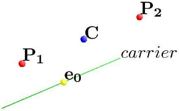
Fig. 1: Conformal point pair $P_{1}\wedge P_{2}$ with center $C$.

This and the following illustrations were produced with the OpenSource visual software CLUCalc [14], which is also based on conformal geometric algebra.

The outer product three conformal points gives a circle (cf. Fig. 2)

$$Circle=P_{1}\wedge P_{2}\wedge P_{3}.$$ (24)

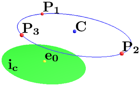
Fig. 2: Conformal circle $P_{1}\wedge P_{2}\wedge P_{3}$ with center $C$.

The conformal outer product of four conformal points gives a sphere (cf. Fig. 3)

$$Sphere = P_{1}\wedge P_{2}\wedge P_{3}\wedge P_{4}.$$ (25)

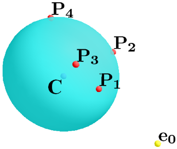
Fig. 3: Conformal sphere $P_{1}\wedge P_{2}\wedge P_{3}\wedge P_{4}$ with center $C$.

If one of the points is at infinity, we get conformal lines (circles through infinity, cf. Fig. 4)

$$Line =P_{1}\wedge P_{2}\wedge\mathrm{\mathbf{e}}_{\infty}=Pp\wedge\mathrm{\mathbf{e}}_{\infty}$$

$$=2r(\mathrm{\mathbf{d}}\wedge\mathrm{\mathbf{c}}\mathrm{\mathbf{e}}_{\infty}-\mathrm{\mathbf{d}}E)\propto\mathrm{\mathbf{m}}\,\mathrm{\mathbf{e}}_{\infty}-\mathrm{\mathbf{d}}E,$$ (26)

where $\mathrm{\mathbf{d}}$ is the direction vector of the line and $\mathrm{\mathbf{c}}$ the 3D midpoint between $P_{1}$ and $P_{2}$, $2r=|\mathrm{\mathbf{p}}_{2}-\mathrm{\mathbf{p}}_{2}|$. $\mathrm{\mathbf{c}}$ can be replaced by any point $\mathrm{\mathbf{p}}$ on the line. $\mathrm{\mathbf{m}}=\mathrm{\mathbf{d}}\wedge\mathrm{\mathbf{c}}=\mathrm{\mathbf{d}}\wedge\mathrm{\mathbf{p}}$ is also called bivector moment of the line.

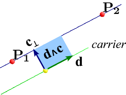
Fig. 4: Conformal line $P_{1}\wedge P_{2}\wedge\mathrm{\mathbf{e}}_{\infty}$ with 3D direction vector $\mathrm{\mathbf{d}}$.

Conformal planes (spheres through infinity, cf. Fig. 5) are represented by

$$Plane=P_{1}\wedge P_{2}\wedge P_{3}\wedge\mathrm{\mathbf{e}}_{\infty}=Circle\wedge\mathrm{\mathbf{e}}_{\infty}.$$ (27)

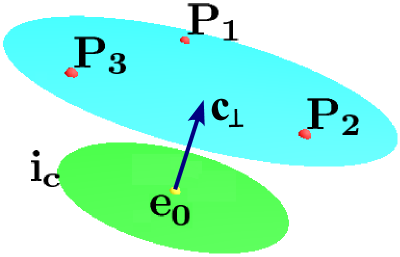
Fig. 5: Conformal plane $P_{1}\wedge P_{2}\wedge P_{3}\wedge\mathrm{\mathbf{e}}_{\infty}$.

Further flattened objects are

$$P\wedge\mathrm{\mathbf{e}}_{\infty},$$ (28)

a (flat) finite–infinite point pair, and

$$-i_{s}E=Sphere\wedge\mathrm{\mathbf{e}}_{\infty}\sim I_{5}=iE,$$ (29)

the in 5D embedded (flat) 3D Euclidean space $\mathbb{R}^{3}$.

2.3 General reflection and motion operators (motors)

As in $\mathcal{G}_{3}$, 3D rotations around the origin in the conformal model $\mathcal{G}_{4,1}$ are still represented by rotors (6). The standard IPNS representation of a conformal plane, i.e. the dual of the direct OPNS representation (27) results in a vector, that both describes the unit normal direction $\mathrm{\mathbf{n}}=\mathrm{\mathbf{c}}_{\perp}/|\mathrm{\mathbf{c}}_{\perp}|$ and the position (signed distance $d=\mathrm{\mathbf{c}}_{\perp}\cdot\mathrm{\mathbf{n}}$ from the origin) of a plane by

$$\mu=Plane^{\ast}=\mathrm{\mathbf{n}}+d\mathrm{\mathbf{e}}_{\infty}.$$ (30)

We can reflect the conformal point $X$ at the general plane (30) similar to (5) with

$$X^{\prime}=-\mu^{-1}X\mu.$$ (31)

A reflection of a general conformal object $O$ (point, point pair, line, …, sphere) at the general plane (30) similar to (31) with

$$O^{\prime}=\mu^{-1}\widehat{O}\mu,$$ (32)

where the grade involution takes care of the sign changes. Just as we obtained rotations (6) by double reflections we now obtain rotations around arbitrary axis (lines of intersection of two planes) by double reflections at planes $\mu_{1}$ and $\mu_{2}$

$$X^{\prime}=R^{-1}XR,\qquad R=\mu_{1}\mu_{2}.$$ (33)

And if the two planes $\mu_{1}$ and $\mu_{2}$ happen to be parallel, i.e. $\mathrm{\mathbf{n}}_{1}=\pm\mathrm{\mathbf{n}}_{2}$, we instead get a translation by twice the Euclidean distance $\mathrm{\mathbf{t}}/2$ between the planes

$$X^{\prime}=T^{-1}XT,$$

$$T(\mathrm{\mathbf{t}})=\mu_{1}\mu_{2}=1+\frac{1}{2}\mathrm{\mathbf{t}}\mathrm{\mathbf{e}}_{\infty}=\exp(\frac{1}{2}\mathrm{\mathbf{t}}\mathrm{\mathbf{e}}_{\infty}).$$ (34)

A general motion operator (motor) results from combining rotations (33) and translations (2.3) to

$$M=TR.$$ (35)

The standard IPNS representation of a sphere results in the vector

$$\sigma=S^{\ast}=C-\frac{1}{2}r^{2}\mathrm{\mathbf{e}}_{\infty},$$ (36)

which is exactly the dual $S^{\ast}=S\,i_{3}^{-1}E$ of (25). The expression (36) shows that in conformal GA a point can be regarded as a sphere with zero radius. We can reflect (invert) the conformal point $X$ at the sphere (36) [or at a conformal point] similar to (5) and (31) simply by

$$X^{\prime}=-\sigma^{-1}X\sigma.$$ (37)

The double reflection at two concentric spheres $\sigma_{1}$ and $\sigma_{2}$ (centered at $\mathrm{\mathbf{c}}$) results in a rescaling operation [8] with factor $s$ and center $\mathrm{\mathbf{c}}$

$$X^{\prime}=Z^{-1}XZ,$$

$$Z=\sigma_{1}\sigma_{2}=T^{-1}(\mathrm{\mathbf{c}})\exp{(E\,\frac{1}{2}\log s)}\,T(\mathrm{\mathbf{c}}).$$ (38)

Table 1 summarizes the various reflections possible in conformal GA.

Table 1: Summary of reflections $O\rightarrow-W^{-1}\widehat{O}W$ in conformal GA. $O$ is a general conformal object (point, point pair, circle, sphere, flat point, line, plane, 3D space). The conformal versor $W$ represents the mirror.

Mirror	Versor $W$
plane	$\mathrm{\mathbf{n}}+d\mathrm{\mathbf{e}}_{\infty}$
point	$\mathrm{\mathbf{p}}+\frac{1}{2}p^{2}\mathrm{\mathbf{e}}_{\infty}+\mathrm{\mathbf{e}}_{0}$
sphere	$C-\frac{1}{2}r^{2}\mathrm{\mathbf{e}}_{\infty}$
line	$\mathrm{\mathbf{m}}\,\mathrm{\mathbf{e}}_{\infty}-\mathrm{\mathbf{d}}E$

Table 2 summarizes the motions and scaling possible in conformal GA.

Table 2: Summary of motions and scaling $O\rightarrow W^{-1}{O}W$ in conformal GA. $O$ is a general conformal object (point, point pair, circle, sphere, flat point, line, plane, 3D space). The conformal versor $W$ represents the motion operator.

Motion operator	Versor $W$
Rotor	$exp(\theta\mathrm{\mathbf{i}}/2)$
Translator	$\exp(\frac{1}{2}\mathrm{\mathbf{t}}\mathrm{\mathbf{e}}_{\infty})$
Motor	$TR$
Scale operator	$T^{-1}(\mathrm{\mathbf{c}})\exp{(E\,\frac{1}{2}\log s)}\,T(\mathrm{\mathbf{c}})$

2.4 Combining elementary transformations

All operations in Tables 1 and 2 can be combined to give further geometric transformations, like rotoinversions, glide reflections, etc.! Algebraically the combination is represented by simply computing the product of the multivector versors of the elementary transformations explained above. Figure 6 shows some examples of combinations of geometric transformations applied to a point pair $P_{1}\wedge P_{2}$. The overbars abbreviate the inverse of an operator.

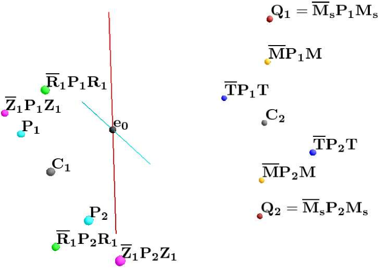
Fig. 6: Examples of combinations of geometric transformations: rotor $R$, translator $T$, scaling operator $Z$, motor and scaling op. $M_{s}$.

The following illustrations have been produced with the socalled Space Group Visualizer [15], a symmetry visualization program for crystallographic space group, which is also based on conformal geometric algebra software.

Figure 7 shows a glide reflection, i.e. a reflection combined with a translation parallel to the plane of reflection.

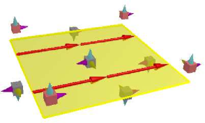
Fig. 7: Examples of glide reflection, which is a reflection combined with a translation parallel to the plane of reflection.

Figure 8 shows a point inversion.

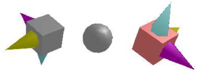
Fig. 8: Examples of point inversion.

Figure 9 shows a screw transformation, which is a rotation followed by a translation along the axis of the rotation.

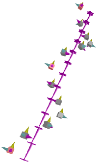
Fig. 9: Examples of a screw transformation.

Figure 10 shows a rotoinversion, which is a combination of point inversion and rotation. A rotoinversion is also equivalent to a rotation followed by a reflection at a plane perpendicular to the axis of rotation.

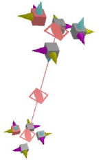
Fig. 10: Examples of a 90 degree rotoinversion, which is a combination of point inversion and a 90 degree rotation.

3. Geometric neurons

Conformal versors $V$ describe in conformal Clifford group  [10] representations the above mentioned transformations of arbitrary conformal geometric object multivectors $X\in\mathcal{G}(\mathbb{R}^{3+1,1})$ of section 2.2

$$X^{\prime}=(-1)^{v}V^{-1}XV,$$ (39)

where the versor is a geometric product of $v$ invertible vectors $\in\mathbb{R}^{3+1,1}$.

The geometric neuron (GN) is characterized by a two-sided multiplication of a single multivector weight versor $W\in\mathcal{G}(\mathbb{R}^{3+1,1})$, input multivectors $X\in\mathcal{G}(\mathbb{R}^{3+1,1})$, and multivector thresholds $\Theta\in\mathcal{G}(\mathbb{R}^{3+1,1})$

$$Y=(-1)^{w}W^{-1}X{W}+\Theta,$$ (40)

where $w$ represents the number of vector factors (parity) in $W$. The theory, optimization and example simulation of such geometric neurons has been studied in [13]. It was shown that e.g. the inversion at a sphere can be learned exactly by a geometric neuron, outperforming linear networks and multilayer perceptrons with the same or higher number of degrees of freedom.

4. Conclusions

We have introduced the concept of geometric algebra as the algebra of a vector space and all its subspaces. We have shown how conformal geometric algebra embeds and models Euclidean geometry. Outer products of points (including the point at infinity) model the elementary geometric objects of points, point pairs, flat points, circles, lines, spheres, planes and the embedded 3D space itself.

The unified representation of affine Euclidean transformations (including translations) by orthogonal transformations in the conformal model allows the construction of a geometric neuron, whose versor weights can learn these transformations precisely. The transformations were illustrated in detail.

Acknowledgments

The author would like to thank K. Tachibana (COE FCS, Nagoya) and S. Buchholz (Kiel). He further wishes to thank God, the creator: Soli Deo Gloria, and his very supportive family.

References

- [1] A. Hirose, Complex-Val. NNs, Springer, Berlin, 2006.
- [2] S. Buchholz, G. Sommer, Quat. Spin. MLP, Proc. ESANN 2000, d-side pub., pp. 377–382, 2000
- [3] N. Matsui, et al, Quat. NN with geome. ops., J. of Intel. & Fuzzy Sys. 15 pp. 149-1164 (2004).
- [4] E. Hitzer, Multivector Diff. Calc., Adv. Appl. Cliff. Alg. 12(2) pp. 135-182 (2002).
- [5] D. Hestenes, G. Sobczyk, Cliff. Alg. to Geom. Calc., Kluwer, Dordrecht, 1999.
- [6] S. Buchholz, A Theory of Neur. Comp. with Cliff. Alg., TR No. 0504, Univ. of Kiel, May 2005.
- [7] D. Hestenes, H. Li, A. Rockwood, New Alg. Tools for Class. Geom., in G. Sommer (ed.), Geom. Comp. with Cliff. Alg., Springer, Berlin, 2001.
- [8] L. Dorst, D. Fontijne, S. Mann, Geom. Alg. for Comp. Sc., Morgan Kaufmann Ser. in Comp. Graph., San Francisco, 2007.
- [9] P. Angles, Conf. Groups in Geom. and Spin Struct., PMP, Birkhauser, Boston, 2007.
- [10] P. Lounesto, Cliff. Alg. and Spinors, 2nd ed., CUP, Cambridge, 2006.
- [11] S. Buchholz, K. Tachibana, E. Hitzer, Optimal Learning Rates for Cliff. Neurons, in LNCS 4668, Springer, Berlin, 2007, pp. 864–873.
- [12] E. Hitzer, et al. Carrier method f. gen. eval. & control of pose, molec. conform., tracking, and the like acc. Adv. in Appl. Cliff. Algs., 26 pp. (2008).
- [13] S. Buchholz, E. Hitzer, K. Tachibana, Coordinate independent update formulas for versor Clifford neurons Proceedings of Joint Conference SCIS & ISIS 2008, Nagoya, Japan, pp. 814–819, (2008).
- [14] C. Perwass, Visual Calculator CLUCalc, http://www.clucalc.info
- [15] C. Perwass, E. Hitzer, Space Group Visualizer, http://www.spacegroup.info