Modelling elastic structures with strong nonlinearities with application to stick-slip friction

Robert Szalai University of Bristol, Queen’s Bldg., University Walk, Bristol, BS8 1TR, UK, email: r.szalai@bristol.ac.uk
(5th September 2013)
Abstract

An exact transformation method is introduced that reduces the governing equations of a continuum structure coupled to strong nonlinearities to a low dimensional equation with memory. The method is general and well suited to problems with point discontinuities such as friction and impact at point contact. It is assumed that the structure is composed of two parts: a continuum but linear structure and finitely many discrete but strong nonlinearites acting at various contact points of the elastic structure. The localised nonlinearities include discontinuities, e.g., the Coulomb friction law. Despite the discontinuities in the model, we demonstrate that contact forces are Lipschitz continuous in time at the onset of sticking for certain classes of structures. The general formalism is illustrated for a continuum elastic body coupled to a Coulomb-like friction model.

I Background

One of the greatest concerns of engineers is modelling friction and impact. These two strong nonlinearities occur in many mechanical structures, e.g., underplatform dampers of turbine blades (Firrone, 2009; Petrov, 2008), tyre models (Pacejka & Besselink, 1997), or in general any jointed structure (Quinn, 2012; Segalman, 2006). The most common way of modelling such systems is to take a finite dimensional approximation assuming that the omitted dynamics has only a small effect on the overall result. Such models can then be analysed using the well established theory of non-smooth dynamical systems (di Bernardo et al., 2008; Filippov & Arscott, 2010). The application of this theory to engineering structures provides a great insight, even though not all phenomena could be experimentally confirmed (Oestreich et al., 1997). Recent results however indicate significant deficiencies that question the predictive power of finite dimensional non-smooth models. It was shown that when a rigid constraint becomes slightly compliant in a friction-type system small-scale instabilities develop (Sieber & Kowalczyk, 2010). This means that refining the model by including more degrees of freedom can lead to qualitatively disagreeing results. The solution can also become non-deterministic (Colombo & Jeffrey, 2011; Nordmark et al., 2011) or non-unique in forward time for an otherwise well specified initial condition. Therefore a better modelling framework is necessary that either eliminates inconsistency and non-determinism or at least provides a hint about the physical mechanism that causes such behaviour.

The most apparent problem with finite dimensional non-smooth models of mechanical systems is that they use rigid body dynamics to describe the motion. This includes finite mode approximation of elastic structures, where each mode has a non-zero modal mass (Ewins, 2000). When two contacting elastic bodies slip and then suddenly stick their contact points will experience a jump in acceleration. In case of a finite mass at the contact point, the contact force also has a jump. In reality, however, the mass of the contact point or contact surface is zero, which implies that the contact force must be continuous. For this reason standard finite mode description of elastic bodies is qualitatively inaccurate. The continuity of contact force should be preserved by mechanical models.

In this paper we propose a formalism that helps better understand and perhaps solve the above problems. We investigate mechanical systems that consist of linear elastic structures coupled at isolated points of contact with strong nonlinearities. This class of problems include mechanisms with Coulomb-like friction models. The dynamics of impact is considered in a companion paper (Szalai, 2013). Our formalism accounts for the zero mass of the contact point without artificially introducing coupling springs as in (Melcher et al., 2013) to regularise the problem. To achieve such model reduction and still provide an exact description we introduce memory terms. Within this new framework the dynamics is described by a low-dimensional delay equation. We show that in our formulation contact forces are Lipschitz or continuous for certain classes of structures when the solution transitions onto the discontinuity surface. The new formalism also leads to well defined dynamics, since small perturbations of the reduced model do not affect the qualitative features of the dynamics in general.

Time-delayed models have already been in use when modelling friction (Hess & Soom, 1990; Putelat et al., 2011). In these cases, however the delay parameters are fitted to experimental observations. We hope that through our theory these empirical parameters can gain physical meaning.

The paper is organised as follows. In section II we present our general mechanical model. In section III we describe our model reduction technique, discuss the convergence of the method and its implications to non-smooth systems. The derivation of the memory term is illustrated through the examples of a pre-tensed string and a cantilever beam. In section V we present the example of a bowed string. We demonstrate the properties of the transformed equation of motion in particular its convergence as the number of vibration modes goes to infinity.

II Mechanical model

Refer to caption
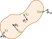
Figure II.1: (colour online) A linear elastic structure with contact points $\chi_{j}$. Each contact point has a three-dimensional motion, however we project that motion to vectors $\boldsymbol{\phi}_{j}$ to obtain a scalar valued resolved variable $y_{j}$. If we need to resolve more than one direction of the motion of the contact point $\chi_{j}$, we attach multiple labels $\chi_{j}=\chi_{j+1}=\chi_{j+2}$ to the same point. Then the motion is projected by the linearly independent vectors $\phi_{j},\,\phi_{j+1},\,\phi_{j+2}$ to yield the resolved variables $y_{j},\,y_{j+1},\,y_{j+2}$. By this definition we ensure a one-to-one mapping between indices of labels $\chi_{j}$ and vectors $\phi_{j}$.

The mechanical model of our structure is divided into two parts, a linear elastic body and several discrete non-smooth nonlinearities that are coupled to the continuum structure. First we describe our assumptions on the linear but infinite dimensional part of the model and then we explain how non-smooth nonlinearities are coupled to the system. The description is sufficiently general to describe friction oscillators and impact phenomena. For simplicity, we only focus on a single elastic structure, but our framework is trivially extensible to mechanisms involving multiple linear structures coupled at (strongly) nonlinear joints.

We assume that the displacement of a material point $\chi$ of the structure at time $t$ is represented by $\boldsymbol{u}(\chi,t)$. We also assume that the motion $\boldsymbol{u}(\chi,t)$ can be expressed as a series

$$\boldsymbol{u}(\chi,t)=\sum_{k=1}^{\infty}\boldsymbol{\psi}_{k}(\chi)x_{k}(t),$$ (II.1)

where $\boldsymbol{\psi}_{k}(\chi)$ are three dimensional vector valued functions depending on the spatial coordinates of the structure only. The generalised coordinates $x_{k}$ can be arranged into a vector $\boldsymbol{x}=(x_{1},x_{2},\ldots)^{T}\in\mathbb{R}^{\infty}$ to simplify the notation. Due to linearity the governing equations can be written as

$$\ddot{\boldsymbol{x}}(t)+\boldsymbol{C}\dot{\boldsymbol{x}}(t)+\boldsymbol{K}\boldsymbol{x}(t)=\boldsymbol{f}_{e}(t),$$ (II.2)

where $\boldsymbol{C}$ and $\boldsymbol{K}$ are the damping and stiffness matrices, respectively, both assumed being multiplied by the inverse mass matrix from the left. The forcing term $\boldsymbol{f}_{e}(t)$ acts as a placeholder for the non-smooth part of the system and will be replaced with with specific terms. Equation (II.2) allows for internal resonances. We assume that these resonances are restricted to arbirarily large but finite dimensional subspaces of the state space, which is necessary to guarantee basic convergence properties of the solution $\boldsymbol{x}(t)$ as shown in appendix C. We also assume that (II.2) is stable in the Lyapunov sense for the same reason.

When $\boldsymbol{C}$ and $\boldsymbol{K}$ matrices are simultaneously diagonalisable the equation of motion can be written in the form of

$$\ddot{\boldsymbol{x}}(t)+2\boldsymbol{D}\boldsymbol{\Omega}\dot{\boldsymbol{x}}(t)+\boldsymbol{\Omega}^{2}\boldsymbol{x}(t)=\boldsymbol{f}_{e}(t),$$ (II.3)

where $\boldsymbol{\Omega}=\mathrm{diag}(\omega_{1},\omega_{2},\ldots)$ and $\boldsymbol{D}=\mathrm{diag}(D_{1},D_{2},\ldots)$. In the unforced case ($\boldsymbol{f}_{e}=\boldsymbol{0}$), the vector components of $\boldsymbol{x}$ on the left side of equation (II.3) are decoupled, which means that the homogeneous equation can be solved for each $x_{k}$ independently. Therefore $x_{k}(t)$ and $\boldsymbol{\psi}_{k}(\chi)$ are called the modes and mode shapes of the system, respectively, with $\omega_{k}$ natural frequencies and $D_{k}$ damping ratios (Ewins, 2000). System (II.3) are called modal equations describing the motion through the modal coordinates $\boldsymbol{x}$. Our results do not require that the equations of motion assume the form (II.3), however in section III.5 some restriction on the eigenvalues of (II.2) is necessary to characterise the convergence of the reduced equations of motion.

In order to take into account the coupling of the contact points to non-smooth nonlinearities we need to characterise their motion. For simplicity we assume point contact. Let us denote the motion of the $j$-th contact point at $\chi_{j}$ along the direction of vector $\boldsymbol{\phi}_{j}$ by

$$y_{j}(t)=\boldsymbol{\phi}_{j}\cdot\boldsymbol{u}(\chi_{j},t)$$ (II.4)

as illustrated in Fig. II.1. We call the positions $y_{j}(t)$ and the velocities $\dot{y}_{j}(t)$ of the contact points resolved variables. We assume $M$ contact points, thus we define $\boldsymbol{y}=(y_{1},\ldots,y_{M},\dot{y}_{1},\ldots,\dot{y}_{M})^{T}$. Substituting (II.1) into (II.4) we obtain the motion of the contact points as a function of the solution of equation (II.2)

$$y_{j}(t)=\boldsymbol{n}{}_{j}\cdot\boldsymbol{x}(t),$$ (II.5)

where

$$\boldsymbol{n}{}_{j}=\left(\boldsymbol{\phi}_{j}\cdot\boldsymbol{\psi}_{1}(\chi_{j}),\boldsymbol{\phi}_{j}\cdot\boldsymbol{\psi}_{2}(\chi_{j}),\ldots\right)^{T}.$$ (II.6)

Vectors $\boldsymbol{n}{}_{j}$ are assumed to be linearly independent, spanning an $M$ dimensional subspace of $\mathbb{R}^{\infty}$.

The nonlinearities are incorporated into the model through the forcing term $\boldsymbol{f}_{e}(t)$. We assume that the nonlinearities only depend on the resolved variables. They are also piecewise continuous with isolated discontinuities. Thus the contact forces acting at contact points $\chi_{j}$ in the direction $\boldsymbol{\phi}_{j}$ are written as $f_{j}(\boldsymbol{y}(t),t).$ Summing up all the nonlinearities completes our model description by providing the right-hand side of equation (II.3) in the form of

$$\boldsymbol{f}_{e}(t)=\sum_{j=1}^{M}\boldsymbol{n}_{j}f_{j}(\boldsymbol{y}(t),t).$$ (II.7)

III Reduction of the mechanical model

We aim to reduce the number of dimensions of our mechanical model (II.7) to an equation that only involves the $2M$ number of resolved variables all contained in the vector $\boldsymbol{y}$. To achieve this we use the Mori-Zwanzig formalism (Chorin et al., 2000) to arrive at a $2M$ dimensional first order delay equation. The solution of the reduced system agrees with the solution of the full system for the resolved variables, while the rest of the variables are discarded. Our method can be viewed as a way of producing a Green’s function for only parts of the system. In this formalism a convolution with the resolved variables represents the effect of the eliminated variables on the dynamics of the resolved variables. The technical details of the transformation are described in appendices A and B.

To simplify our calculation we transform equation (II.3) into a first order form of

$$\dot{\boldsymbol{z}}(t)=\boldsymbol{R}\boldsymbol{z}(t)+\boldsymbol{f}(t),$$ (III.1)

where

$$\boldsymbol{R}=\left(\begin{array}[]{cc}\boldsymbol{0}&\boldsymbol{I}\\ -\boldsymbol{K}&-\boldsymbol{C}\end{array}\right)\;\mbox{and}\;\boldsymbol{f}(t)=\left(\begin{array}[]{c}\boldsymbol{0}\\ \boldsymbol{f}_{e}(t)\end{array}\right).$$ (III.2)

We already have a way of obtaining the resolved variables from the generalised coordinates $\boldsymbol{x}$ through a dot product with vectors $\boldsymbol{n}{}_{j}$ as shown in equation (II.5). In a matrix-vector notation we write the conversion as

$$\boldsymbol{y}(t)=\boldsymbol{V}\boldsymbol{z}(t),\;\mbox{with}\;\boldsymbol{V}=\left(\begin{array}[]{c}\boldsymbol{v}_{1}^{T}\\ \vdots\\ \boldsymbol{v}_{2M}^{T}\end{array}\right)\,\mbox{and}\,\boldsymbol{v}_{j}=\left(\begin{array}[]{c}\boldsymbol{n}_{j}\\ \boldsymbol{0}\end{array}\right),\;\boldsymbol{v}_{M+j}=\left(\begin{array}[]{c}\boldsymbol{0}\\ \boldsymbol{n}_{j}\end{array}\right).$$ (III.3)

To obtain our reduced model we construct a projection matrix $\boldsymbol{S}$ that acts on the generalised coordinates and has a $2M$ dimensional range. In order to do that we also define a lifting operator in the form of

$$\boldsymbol{z}(t)=\boldsymbol{W}\boldsymbol{y}(t),\;\mbox{with\;}\boldsymbol{W}=\left(\begin{array}[]{ccc}\boldsymbol{w}_{1}&\cdots&\boldsymbol{w}_{2M}\end{array}\right).$$ (III.4)

Note that the lifting operator with $\boldsymbol{W}$ does not reproduce the full solution from the resolved variables, it is merely used as a technical tool. Moreover, $\boldsymbol{W}$ does not depend on the physical system, it can be chosen to suite the reduction procedure. By combining matrices $\boldsymbol{V}$ and $\boldsymbol{W}$ we obtain our projections $\boldsymbol{S}=\boldsymbol{W}\boldsymbol{V}$ and $\boldsymbol{Q}=\boldsymbol{I}-\boldsymbol{S}$ on the condition that $\boldsymbol{m}_{k}$ satisfy $\boldsymbol{m}_{k}\cdot\boldsymbol{n}_{l}=0$ if $k\neq l$ and $\boldsymbol{m}_{k}\cdot\boldsymbol{n}_{k}=1$. This constraint can also be expressed as $\boldsymbol{I}=\boldsymbol{V}\boldsymbol{W}$ (note the order of the two matrices).

To guarantee that the terms in the reduced equation are bounded the choice of $\boldsymbol{W}$ needs to be further restricted. Therefore we assume that the range of $\boldsymbol{W}$ is invariant under $\boldsymbol{R}$, that is,

$$\boldsymbol{R}\boldsymbol{w}_{j}\in\mathrm{span}(\boldsymbol{w}_{1},\boldsymbol{w}_{2},\ldots,\boldsymbol{w}_{2M}),\;\mbox{for}\;j=1,2,\ldots,2M.$$ (III.5)

Equivalently, $\boldsymbol{w}_{j}$ can be constructed as linear combinations of $2M$ number of eigenvectors of $\boldsymbol{R}$, since eigenvectors are invariant by definition. This assumption is key to our analysis.

In case of the modal equations (II.3) the columns of $\boldsymbol{W}$ can be explicitly constructed in the form of

$$\boldsymbol{w}_{j}=\left(\begin{array}[]{c}\boldsymbol{m}_{j}\\ \boldsymbol{0}\end{array}\right)\;\mbox{and}\;\boldsymbol{w}_{M+j}=\left(\begin{array}[]{c}\boldsymbol{0}\\ \boldsymbol{m}_{j}\end{array}\right).$$ (III.6)

Due to the block diagonal form of $\boldsymbol{R}$ condition (III.5) holds when the $\boldsymbol{m}_{j}$ vectors are chosen such that they only have $M$ number of non-zero components:

$$\left[\boldsymbol{m}_{j}\right]_{p}=0,\quad\mbox{for}\quad p<P\;\mbox{and}\;p\geq P+M.$$ (III.7)

As the last step before arriving at the reduced equations we define

$\displaystyle\boldsymbol{A}$ $\displaystyle=\boldsymbol{V}\boldsymbol{R}\boldsymbol{W},$ $\displaystyle\in\mathbb{R}^{2M\times 2M}$ (III.8)
$\displaystyle\boldsymbol{H}(t)\boldsymbol{z}(s)$ $\displaystyle=\boldsymbol{V}\boldsymbol{R}\boldsymbol{Q}\mathrm{e}^{\boldsymbol{R}(t-s)}\boldsymbol{z}(s),$ $\displaystyle\in\mathbb{R}^{2M}$ (III.9)
$\displaystyle\boldsymbol{L}_{j}(\tau)$ $\displaystyle=\boldsymbol{V}\mathrm{e}^{\boldsymbol{R}\tau}\boldsymbol{v}_{M+j}-\boldsymbol{A}\boldsymbol{V}\int_{0}^{\tau}\mathrm{e}^{\boldsymbol{R}\theta}\boldsymbol{v}_{M+j}\mathrm{d}\theta,$ $\displaystyle\in\mathbb{R}^{2M}$ (III.10)

where $\boldsymbol{z}(s)$ is the initial condition of equation (III.1) at time $s$ and $\mathrm{e}^{\boldsymbol{R}t}$ is the fundamental matrix of equation (III.1). The matrix $\boldsymbol{A}$ is bounded if condition (III.5) holds, while $\boldsymbol{H}(t)\boldsymbol{z}(s)$ is bounded if the initial condition $\boldsymbol{z}(s)$ is bounded, too. To obtain the memory kernel $\boldsymbol{L}_{j}(\tau)$, one needs to solve the first order system (III.1) for $M$ different initial conditions $\boldsymbol{v}_{M+j}$. This solution may not be bounded which we rectify by integrating it (see sections III.2 and III.5).

Using the expression (II.7) of the forcing term our reduced equation that is equivalent to (III.1) in the resolved variables becomes

$$\dot{\boldsymbol{y}}(t)=\boldsymbol{A}\boldsymbol{y}(t)+\sum_{j=1}^{M}\left[\boldsymbol{L}_{j}(0)f_{j}(\boldsymbol{y}(t),t)+\int_{0}^{t-s}\mathrm{d}_{\tau}\boldsymbol{L}_{j}(\tau)f_{j}(\boldsymbol{y}(t-\tau),t-\tau)\right]+\boldsymbol{H}(t)\boldsymbol{z}(s),$$ (III.11)

where the integral is understood in the Riemann-Stieltjes sense (see section III.1). The formal equivalence of (III.1) and (III.11) is proved in appendix A and the formulae of $\boldsymbol{A}$, $\boldsymbol{H}(t)\boldsymbol{z}(s)$ and $\boldsymbol{L}_{j}(\tau)$ are derived in appendix B. It turns out that for mechanical systems the alternative form of (III.11) given below by equation (III.20) is more appropriate.

III.1 The meaning of the Riemann-Stieltjes integral

To provide some intuition about the interpretation of the integral in (III.11) we remark that if $\boldsymbol{L}_{j}(\tau)$ is differentiable, the symbol $\mathrm{d}_{\tau}\boldsymbol{L}_{j}(\tau)$ can be replaced by $\nicefrac{{\mathrm{d}}}{{\mathrm{d}\tau}}\boldsymbol{L}_{j}(\tau)\cdots\mathrm{d}\tau$ to arrive at an ordinary Riemann integral. Similar simplification can be achieved if $\boldsymbol{L}_{j}(\tau)$ is Lipschitz continuous, however $\mathrm{d}_{\tau}\boldsymbol{L}_{j}(\tau)$ is replaced by the left derivative of $\boldsymbol{L}_{j}(\tau)$. A discontinuity of $\boldsymbol{L}_{j}(\tau)$ at $\tau^{\star}$ translates into a discrete delay term $\mathfrak{L}_{j}(\tau^{\star})f_{j}(\boldsymbol{y}(t-\tau^{\star}),t-\tau^{\star})$, where $\mathfrak{L}_{j}(\tau^{\star})$ is the gap in the function at $\tau^{\star}$. Therefore if $\boldsymbol{L}_{j}(\tau)$ is piecewise differentiable (or piecewise Lipschitz), with finite number of isolated discontinuities, the integral in (III.11) can be replaced by a sum of Riemann integrals and discrete delays. In particular, assuming that the discontinuities occur at $\tau_{p}^{\star}$, $p=1,\ldots,P$ and that $\tau_{0}^{\star}=0$ and $\tau_{P+1}^{\star}=t$ we can write

$$\int_{0}^{t-s}\mathrm{d}_{\tau}\boldsymbol{L}_{j}(\tau)f(t-\tau)\mathrm{d}\tau=\sum_{p=0}^{P}\int_{\tau_{p}^{\star}}^{\tau_{p+1}^{*}-s}\left[\frac{\mathrm{d}}{\mathrm{d}\tau}\boldsymbol{L}_{j}(\tau)\right]f(t-\tau)\mathrm{d}\tau+\sum_{p=1}^{P}\mathfrak{L}_{j}(\tau_{p}^{\star})f(t-\tau_{p}^{\star}),$$ (III.12)

where $\mathfrak{L}_{j}(\tau^{\star})=\lim_{\tau\to\tau*+0}\boldsymbol{L}_{j}(\tau)-\lim_{\tau\to\tau*-0}\boldsymbol{L}_{j}(\tau)$.

One can interpret the memory kernels $\boldsymbol{L}_{j}(\tau)$ as an indication how waves travel within the structure from contact point $\chi_{j}$ to all contact points including them returning to $\chi_{j}$. Indeed, the tail part of $\boldsymbol{L}_{j}(\tau)$ for $\tau>0$ describes how a force applied in the past is affecting the contact points at current time. This notion is therefore analogous to having waves that depart from point $\chi_{j}$ and arrive at all contact points $\chi_{l}$, $l=1,\ldots,M$ $\tau$ time later. In particular if waves do not disperse, they arrive simultaneously at a give material point $\chi_{l}$ exactly $\tau^{\star}$ time later and that corresponds to a discrete delay represented by a discontinuity in $\boldsymbol{L}_{j}(\tau)$ at $\tau=\tau^{\star}$.

The time delay in (III.11) tends to infinity, since the history of $\boldsymbol{y}(t)$ to be taken into account grows with time. However, if $\boldsymbol{L}_{j}(\tau)$ tends to a constant as $\tau\to\infty$, the integrals in (III.11) may be truncated at a finite delay time to produce an approximate model. In case of a conservative equation (II.3), the delay cannot be truncated at a finite time, because the motion of the free structure will never stop due to the conservation of the kinetic energy. This is illustrated in section III.3.

III.2 An alternative form of the reduced equations

It was mentioned before that $\boldsymbol{L}_{j}(\tau)$ may not be a bounded function. Therefore we integrate the convolution in equation (III.11) by parts, so that the integral of $\boldsymbol{L}_{j}(\tau)$ and the derivative of the contact force $f_{j}$ appear in the rewritten equation. However, to be able to integrate $\boldsymbol{L}_{j}(\tau)$ and ensure that the integral does not grow out of bound, we need to decompose $\boldsymbol{L}_{j}(\tau)$ into a constant and an oscillatory term

$$\boldsymbol{L}_{j}(\tau)=\boldsymbol{L}_{j}^{\infty}+\boldsymbol{L}_{j}^{0}(\tau),$$ (III.13)

where

$$\boldsymbol{L}_{j}^{\infty}=\lim_{t\to\infty}\frac{1}{t}\int_{0}^{t}\boldsymbol{L}_{j}(\tau)\mathrm{d}\tau.$$ (III.14)

Since we have a formal expression for $\boldsymbol{L}_{j}(\tau)$ in the form of equation (III.10), we can calculate the integral

$$\int_{0}^{t}\boldsymbol{L}_{j}(\tau)\mathrm{d}\tau=\int_{0}^{t}\left(\boldsymbol{V}\mathrm{e}^{\boldsymbol{R}\tau}-\boldsymbol{A}\boldsymbol{V}\int_{0}^{\tau}\mathrm{e}^{\boldsymbol{R}\theta}\mathrm{d}\theta\right)\mathrm{d}\tau\boldsymbol{v}_{M+j}.$$ (III.15)

From the simple rule of differentiating an exponential we find that $\int_{0}^{\tau}\mathrm{e}^{\boldsymbol{R}\theta}\mathrm{d}\theta=\boldsymbol{R}^{-1}\left(\mathrm{e}^{\boldsymbol{R}\tau}-\boldsymbol{I}\right)$. Using this formula twice in equation (III.15), we are left with

$$\int_{0}^{t}\boldsymbol{L}_{j}(\tau)\mathrm{d}\tau=\left(\boldsymbol{V}\boldsymbol{R}^{-1}\left(\mathrm{e}^{\boldsymbol{R}t}-\boldsymbol{I}\right)-\boldsymbol{A}\boldsymbol{V}\boldsymbol{R}^{-1}\left(\boldsymbol{R}^{-1}\left(\mathrm{e}^{\boldsymbol{R}t}-\boldsymbol{I}\right)-t\right)\right)\boldsymbol{v}_{M+j}.$$ (III.16)

Assuming that $\boldsymbol{V}\int_{0}^{\tau}\mathrm{e}^{\boldsymbol{R}\theta}\mathrm{d}\theta\boldsymbol{v}_{M+j}$ is bounded (see section III.5) the limit (III.14) becomes

$$\boldsymbol{L}_{j}^{\infty}=\boldsymbol{A}\boldsymbol{V}\boldsymbol{R}^{-1}\boldsymbol{v}_{M+j}.$$ (III.17)

Note that $\boldsymbol{V}\boldsymbol{R}^{-1}\boldsymbol{v}_{M+j}$ is the static displacement of the contact points under a static unit load at contact point $\chi_{j}$. Indeed, by expanding equation $\boldsymbol{R}\left(\boldsymbol{x},\boldsymbol{y}\right)^{T}=\left(\boldsymbol{0},\boldsymbol{n}_{j}\right)^{T}$ we get $\boldsymbol{K}\boldsymbol{x}=\boldsymbol{n}_{j}$ and $\boldsymbol{y}=\boldsymbol{0}$, where $\boldsymbol{x}$ is the static displacement of the generalised coordinates, hence, $\boldsymbol{V}\boldsymbol{x}=\boldsymbol{V}\boldsymbol{R}^{-1}\boldsymbol{v}_{M+j}$ is the static displacement of the contact points.

Our definition (III.13) of $\boldsymbol{L}_{j}^{0}(\tau)$ implies that either $\boldsymbol{L}_{j}^{0}(\tau)\to\boldsymbol{0}$ exponentially if the system is dissipative or $\boldsymbol{L}_{j}^{0}(\tau)$ oscillates with zero mean. Therefore we define the integral

$$\boldsymbol{L}_{j}^{1}(t)=\int_{0}^{t}\boldsymbol{L}_{j}^{0}(\tau)\mathrm{d}\tau.$$ (III.18)

The boundedness and smoothness of (III.18) is discussed in section III.5. By virtue of (III.18) the forcing terms in (III.11) can be integrated by parts as follows

$$\boldsymbol{L}_{j}(0)\boldsymbol{f}(t)+\int_{0}^{t-s}\mathrm{d}_{\tau}\boldsymbol{L}_{j}(\tau)f_{j}(\boldsymbol{y}(t-\tau),t-\tau)=\\ =\boldsymbol{L}_{j}^{\infty}f_{j}(t)+\boldsymbol{L}_{j}^{0}(t-s)f_{j}(s)+\int_{0}^{t-s}\mathrm{d}_{\tau}\boldsymbol{L}_{j}^{1}(\tau)\frac{\mathrm{d}}{\mathrm{d}t}[f_{j}(\boldsymbol{y}(t-\tau),t-\tau)],$$ (III.19)

which has only bounded terms if the derivative $\frac{\mathrm{d}}{\mathrm{d}t}[f_{j}(t)]$ exists and is bounded almost everywhere and condition (III.34) in section III.5 holds. Using this transformation the governing equation becomes

$$\dot{\boldsymbol{y}}(t)=\boldsymbol{A}\boldsymbol{y}(t)+\sum_{j=1}^{M}\left[\boldsymbol{L}_{j}^{\infty}f_{j}(t)+\int_{0}^{t-s}\mathrm{d}_{\tau}\boldsymbol{L}_{j}^{1}(\tau)\frac{\mathrm{d}}{\mathrm{d}t}[f_{j}(\boldsymbol{y}(t-\tau),t-\tau)]\right]+\boldsymbol{g}(t),$$ (III.20)

where $\boldsymbol{g}(t)=\boldsymbol{H}(t)\boldsymbol{z}(s)+\sum_{j=1}^{M}\boldsymbol{L}_{j}^{0}(t-s)f_{j}(s).$

It is important to note that according to the theory of delay equations (Hale & Lunel, 1993) if the terms in equation (III.20) are slightly perturbed, the solution of (III.20) changes only slightly under general conditions. This is a clear advantage over the finite dimensional description where perturbation generally leads to qualitatively disagreeing solutions (Sieber & Kowalczyk, 2010).

III.3 Vibrations of a pre-tensed string

Refer to caption
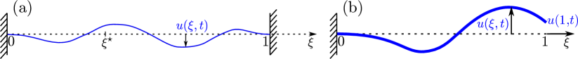
Figure III.1: Schematic of a string (a) and a beam (b). The displacement of material points is described by $u(\xi,t)$, which represents motion in the direction of the arrows.

In this section we illustrate the calculation of $\boldsymbol{A}$ and $\boldsymbol{L}_{j}^{1}(t)$ for a pre-tensed string without bending stiffness. We keep the calculation as general as possible so that it applies to systems with a single contact point that can be written in the form of II.3. The schematic of the string is shown in Fig. III.1(a), whose motion is described by the equation

$$\frac{\partial^{2}u}{\partial t^{2}}=c^{2}\frac{\partial^{2}u}{\partial\xi^{2}}+\delta(\xi-\xi^{\star})F_{c}(t)+\mbox{damping},$$ (III.21)

where $c$ is the wave speed, $u(t,\xi)$ is the deflection of the string, $t$ stands for time and $0\leq\xi\leq 1$ is the coordinate along the string. The boundary conditions $u(0,t)=0$ and $u(1,t)=0$ express that there is no movement at the two ends of the string. Equation (III.21) indicates damping, which explicitly appears in the mode decomposed system (II.3) with non-zero damping ratios. The string is forced at $\xi=\xi^{\star}$ by a contact force $F_{c}(t)$, which is represented by the Dirac delta function in equation (III.21).

The first step is to provide a mode decomposition in the form of equation (II.3), so that the vibration of the string is expressed by (II.1), where the mode shapes are the scalar valued $\psi_{k}(\xi)=\sin\left(k\pi\xi\right)$. The natural frequencies of the system are $\omega_{k}=ck\pi$ and we assume uniform damping $D_{k}=\nicefrac{{1}}{{10}}$ for all modes, which gives us

$$\boldsymbol{\Omega}=\mathrm{diag}(c\pi,c2\pi,\ldots),\quad\mbox{and}\quad\boldsymbol{D}=\mathrm{diag}(\nicefrac{{1}}{{10}},\nicefrac{{1}}{{10}},\ldots).$$ (III.22)

The vibration at the contact point can be expressed as a linear combination of all the modes $u(\xi^{\star},t)=\boldsymbol{n}\cdot\boldsymbol{x}(t)$, where $\boldsymbol{n}=(\sin\left(\pi\xi^{\star}\right),\sin\left(2\pi\xi^{\star}\right),\ldots)^{T}$. The resolved variables therefore are $y_{1}(t)=\boldsymbol{n}\cdot\boldsymbol{x}(t)$ and $y_{2}(t)=\dot{y}_{1}(t)$. We also choose $\boldsymbol{m}=(\nicefrac{{1}}{{\sin\pi\xi^{\star}}},0,0,\ldots)^{T}$ in formula (III.6), thus

$$\boldsymbol{A}=\left(\begin{array}[]{cc}0&1\\ -\omega_{1}^{2}&-2D_{1}\omega_{1}\end{array}\right).$$ (III.23)

Next we calculate the function $\mathrm{e}^{\boldsymbol{R}t}\boldsymbol{v}_{2}$ that appears in the expression (III.10) of $\boldsymbol{L}(\tau)$. The equation whose solution we are seeking is $\dot{\boldsymbol{z}}=\boldsymbol{R}\boldsymbol{z}$, which is expanded into

$$\dot{z}_{1,k}=z_{2,k},\quad\dot{z}_{2,k}=-2D_{k}\omega_{k}z_{2,k}-\omega_{k}^{2}z_{1,k},\quad k=1,2,3,\ldots.$$ (III.24)

The initial conditions that correspond to $\boldsymbol{z}(0)=\boldsymbol{v}_{2}$ are $z_{1,k}(0)=0$ and $z_{2,k}(0)=\left[\boldsymbol{n}\right]_{k}$. The solution for the modes are

$$z_{1,k}(t)=\left[\boldsymbol{n}\right]_{k}\mathrm{e}^{-D_{k}\omega_{k}t}\frac{\sin\sqrt{1-D_{k}^{2}}\omega_{k}t}{\sqrt{1-D_{k}^{2}}\omega_{k}}.$$ (III.25)

Without assuming the form of $z_{1,k}(t)$ and evaluating formula (III.10) we find that

$\displaystyle\left[\boldsymbol{L}(t)\right]_{1}$ $\displaystyle=\boldsymbol{v}_{1}\cdot\mathrm{e}^{\boldsymbol{R}t}\boldsymbol{v}_{2}-\boldsymbol{v}_{2}\cdot\int_{0}^{t}\mathrm{e}^{\boldsymbol{R}\theta}\mathrm{d}\theta\boldsymbol{v}_{2}=0\quad\mbox{and}$
$\displaystyle\left[\boldsymbol{L}(\tau)\right]_{2}$ $\displaystyle=\boldsymbol{v}_{2}\cdot\mathrm{e}^{\boldsymbol{R}t}\boldsymbol{v}_{2}+2D_{1}\omega_{1}\boldsymbol{v}_{1}\cdot\mathrm{e}^{\boldsymbol{R}t}\boldsymbol{v}_{2}+\omega_{1}^{2}\boldsymbol{v}_{1}\cdot\int_{0}^{t}\mathrm{e}^{\boldsymbol{R}\theta}\mathrm{d}\theta\boldsymbol{v}_{2}$
$\displaystyle=\sum_{k=1}^{\infty}\left[\boldsymbol{n}\right]_{k}\left(\frac{d}{dt}z_{1,k}(t)+2D_{1}\omega_{1}z_{1,k}(t)+\omega_{1}^{2}\int_{0}^{t}z_{1,k}(t)d\theta\right).$ (III.26)

Eventually substituting (III.25) into (III.26) in the conservative case ($D_{k}=0$) $\left[\boldsymbol{L}(t)\right]_{2}$ of our system (III.21) becomes

$$\left[\boldsymbol{L}(t)\right]_{2}=\sum_{k=1}^{\infty}\sin^{2}k\pi\xi^{\star}\frac{\omega_{1}^{2}}{\omega_{k}^{2}}+\sum_{k=2}^{\infty}\sin^{2}k\pi\xi^{\star}\left(1-\frac{\omega_{1}^{2}}{\omega_{k}^{2}}\right)\cos\omega_{k}t,$$ (III.27)

which is a divergent Fourier series, therefore equation (III.11) cannot be utilised to describe the dynamics. The constant term in equation (III.26) regardless of the damping ratios assumes the form

$$\left[\boldsymbol{L}^{\infty}\right]_{2}=-\omega_{1}^{2}\boldsymbol{v}_{1}\boldsymbol{R}^{-1}\boldsymbol{v}_{2}=\sum_{k=1}^{\infty}\left[\boldsymbol{n}\right]_{k}^{2}\frac{\omega_{1}^{2}}{\omega_{k}^{2}}.$$ (III.28)

Note that this is $-\omega_{1}^{2}$ times the static displacement of the string under unit load at $\xi=\xi^{\star}$. Using the expressions for $z_{1,k}(t)$ and integrating $\left[\boldsymbol{L}(t)\right]_{2}-\left[\boldsymbol{L}^{\infty}\right]_{2}$ as per definition (III.18) we get

$$\left[\boldsymbol{L}^{1}(\tau)\right]_{2}=\sum_{k=1}^{\infty}\left[\boldsymbol{n}\right]_{k}^{2}\frac{e^{-tD_{k}\omega_{k}}}{\sqrt{1-D_{k}^{2}}\omega_{k}^{3}}\left\{2\omega_{1}^{2}D_{k}\sqrt{1-D_{k}^{2}}\cos\left(t\sqrt{1-D_{k}^{2}}\omega_{k}\right)\right.\\ \left.+\left(\omega_{1}^{2}\left(2D_{k}^{2}-1\right)+\left(2D_{1}\omega_{1}+1\right)\omega_{k}^{2}\right)\sin\left(t\sqrt{1-D_{k}^{2}}\omega_{k}\right)\right\}-\left[\boldsymbol{n}\right]_{k}^{2}\frac{2\omega_{1}^{2}D_{k}}{\omega_{k}^{3}}.$$ (III.29)

Assuming that $D_{k}=D$ are constant, the right limit of $\left[\boldsymbol{L}^{1}(\tau)\right]_{2}$ becomes

$$\lim_{\tau\to 0+}\left[\boldsymbol{L}^{1}(\tau)\right]_{2}=\frac{\cos^{-1}D}{2\pi c\sqrt{1-D^{2}}}$$ (III.30)

The detailed calculation of (III.30) can be found in appendix E, which also indicates the boundedness of $\left[\boldsymbol{L}^{1}(\tau)\right]_{2}$. The graph of $\left[\boldsymbol{L}^{1}(\tau)\right]_{2}$ for $c=1$ is illustrated in Fig. III.2(a) for both the conservative and the damped case.

Refer to caption
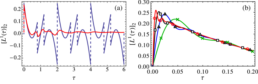
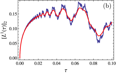
Figure III.2: (colour online) Graph of $\left[\boldsymbol{L}^{1}(\tau)\right]_{2}$ for the string equation (III.21) with at $\xi^{\star}=0.4,$ $c=1$. The blue line represents the conservative case and the red corresponds to the damped case with $D_{k}=\nicefrac{{1}}{{10}}$. (b) Graph of the function $\left[\boldsymbol{L}^{1}(\tau)\right]_{2}$ when truncating the series (III.29) at $20,40,80,160$ terms, denoted by $\times,\triangle,\square$ and $\ocircle$, respectively.

Note that the convolution kernel $\boldsymbol{L}^{1}(\tau)$ for $D_{k}=0$ is periodic and therefore the delay that occurs as the effect of nonlinearities is infinite. If damping is introduced $\boldsymbol{L}^{1}(\tau)$ decays in time so that the past of the system will have a smaller effect. This is illustrated by the red line in Fig III.2(a). For non-zero damping, as an approximation one can truncate the delay to a finite time-interval. Truncation is a reasonable choice for most practical purposes, but it is not quite clear what are the theoretical implications (Farkas & Stépán, 1992).

It is worth noting that equation (III.21) in the conservative case can be solved using D’Alembert’s formula that also leads to a delay-differential equation (Stépán & Szabó, 1999), which is similar to (III.20).

III.4 Euler-Bernoulli cantilever beam

We choose the Euler-Bernoulli beam as our second example to illustrate the theory. This model can support waves of infinite speed, therefore its physical validity is questionable. Nevertheless it is worth investigating how this property of the Euler-Bernoulli beam translates into the properties of the memory kernel. The non-dimensional governing equation and boundary conditions are

$$\frac{\partial^{2}u}{\partial t^{2}}=-\frac{\partial^{4}u}{\partial\xi^{2}}+\mbox{damping},\;u(t,0)=u^{\prime}(t,0)=u^{\prime\prime}(t,1)=u^{\prime\prime\prime}(t,1)=0.$$ (III.31)

The natural frequencies of (III.31) are determined by the equation $1+\cos\sqrt{\omega_{k}}\cosh\sqrt{\omega_{k}}=0$, which can be approximated by $\cos\sqrt{\omega_{k}}\approx 0$ for $\omega_{k}$ sufficiently large. Therefore $\omega_{k}\approx\left(k\pi-\nicefrac{{\pi}}{{2}}\right)^{2}$. We use this estimate as a starting point to numerically find more accurate $\omega_{k}$ values. The mode shapes at the free end of the beam assume the values given by vector $\boldsymbol{n}=(2,-2,2,-2,\ldots)^{T}.$ We choose $\boldsymbol{m}=(\nicefrac{{1}}{{2}},0,0,\ldots)^{T}$ in formula (III.6), so that $\boldsymbol{W}$ satisfies our assumption (III.5).

The general formulae that were derived in section III.3 still apply to equation (III.31) with the appropriate ωksubscript𝜔𝑘\omega_{k}, Dksubscript𝐷𝑘D_{k} and [𝒏]ksubscriptdelimited-[]𝒏𝑘\left[\boldsymbol{n}\right]_{k} values. In particular, we use (III.29) to plot the memory kernel in Fig.
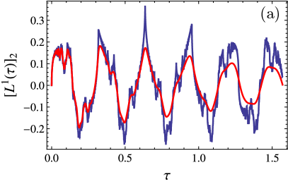
 III.3. The graph of [𝑳1(τ)]2subscriptdelimited-[]superscript𝑳1𝜏2\left[\boldsymbol{L}^{1}(\tau)\right]_{2} in Fig. III.3(a) shows that the quadratically growing natural frequencies make the function non-smooth in the conservative case. When damping is introduced the function becomes smooth for τ>0𝜏0\tau>0. Fig. III.3(b) shows that for 0τ10𝜏much-less-than10\leq\tau\ll 1 [𝑳1(τ)]2subscriptdelimited-[]superscript𝑳1𝜏2\left[\boldsymbol{L}^{1}(\tau)\right]_{2} grows like a power curve τpsuperscript𝜏𝑝\tau^{p}, 0<p<10𝑝10<p<1. Therefore [𝑳1(τ)]2subscriptdelimited-[]superscript𝑳1𝜏2\left[\boldsymbol{L}^{1}(\tau)\right]_{2} is not differentiable at τ=0𝜏0\tau=0.

Refer to caption
Refer to caption
Figure III.3: (colour online) The graph of $\left[\boldsymbol{L}^{1}(\tau)\right]_{2}$ for the Euler-Bernoulli cantilever beam. The blue curves correspond to the conservative case and the red curves represent the damped system with $D_{k}=\nicefrac{{1}}{{50}}$. The conservative case illustrates the lack of smoothness of $\left[\boldsymbol{L}^{1}(\tau)\right]_{2}$ for $\tau>0$. Panel (b) illustrates that $\left[\boldsymbol{L}^{1}(\tau)\right]_{2}$ is not differentiable at $\tau=0$.

III.5 The convergence of $\boldsymbol{L}_{j}^{1}(\tau)$

So far we derived the reduced equation of motion (III.20) without any consideration whether intermediate terms are well-defined. To make the analysis rigorous we introduce infinite dimensional vector spaces

$$\boldsymbol{X}=\{\boldsymbol{x}\in\mathbb{R}^{\infty}:\sum_{i}x_{i}^{2}<\infty\}\;\mbox{and}\;\boldsymbol{Z}=\boldsymbol{X}^{2}$$ (III.32)

that contain the solutions of the second (II.2) and first order system (III.1), respectively. One can check that in the previous two examples $\boldsymbol{v}_{M+j}\notin\boldsymbol{Z}$, because their norm is infinite. This also implies that $\left\|\boldsymbol{V}\right\|=\infty$. Even if we know that $\left\|\mathrm{e}^{\boldsymbol{R}\tau}\right\|\leq M_{0}<\infty$, the bound of $\boldsymbol{L}_{j}^{1}(\tau)$ cannot be directly estimated in the straightforward way, because $\left\|\boldsymbol{V}\mathrm{e}^{\boldsymbol{R}\tau}\boldsymbol{v}_{M+j}\right\|\leq\left\|\boldsymbol{V}\right\|\left\|\mathrm{e}^{\boldsymbol{R}\tau}\right\|\left\|\boldsymbol{v}_{M+j}\right\|=\infty$. However the two examples in the previous sections show that $\boldsymbol{L}_{j}^{1}(\tau)$ can be bounded, but not necessarily smooth. In case of the string and without damping, $\boldsymbol{L}_{j}^{1}(\tau)$ is a piecewise-smooth function, while $\boldsymbol{L}_{j}^{1}(\tau)$ appears to be continuous but non-differentiable for the undamped Euler-Bernoulli beam. If damping is introduced, $\boldsymbol{L}_{j}^{1}(\tau)$ becomes smooth for $\tau>0$ and discontinuity or non-differentiability occurs only at $\tau=0$ in both examples.

Boundedness and smoothness depends on the eigenvalues of $\boldsymbol{R}$, which are directly related to the natural frequencies and damping ratios of system (II.2). First we assume that all the eigenvalues $\sigma(\boldsymbol{R})$ are in the left half of the complex plane including the imaginary axis, that is,

$$\sigma(\boldsymbol{R})\subset\{\lambda\in\mathbb{C}:\Re\lambda\leq 0\}.$$ (III.33)

This guarantees that $\mathrm{e}^{\boldsymbol{R}t}$ is a strongly continuous semigroup with $\left\|\mathrm{e}^{\boldsymbol{R}t}\right\|\leq C_{0}$ as shown in appendix C. This does not guarantee continuity or boundedness of $\boldsymbol{L}_{j}^{1}(\tau)$, but it is a necessary condition. However when condition

$$\left|\lambda\boldsymbol{n}_{l}\cdot(\boldsymbol{K}+\lambda\boldsymbol{C}+\lambda^{2})^{-1}\boldsymbol{n}_{j}\right|\leq M_{j,l}\;\mbox{for}\;\lambda\in\{\mathbb{C}:\Re\lambda=\gamma>0\}$$ (III.34)

is satisfied as well, appendix D shows that $\boldsymbol{L}_{j}^{1}(\tau)$ is bounded.

Smoothness of $\boldsymbol{L}_{j}^{1}(\tau)$ can be guaranteed if we replace (III.33) and (III.34) with a stronger assumptions. We assume that there exists a $D_{0}>0$ such that the eigenvalues of $\boldsymbol{R}$ satisfy

$$\sigma(\boldsymbol{R})\subset\{\lambda\in\mathbb{C}:\Re(\lambda)\leq-D_{0}\left|\Im(\lambda)\right|\},$$ (III.35)

in other words the eigenvalues of $\boldsymbol{R}$ are contained in a sector of the imaginary half-plane. Instead of (III.34) we assume that

$$\left|\lambda\boldsymbol{n}_{l}\cdot(\boldsymbol{K}+\lambda\boldsymbol{C}+\lambda^{2})^{-1}\boldsymbol{n}_{j}\right|\leq M_{j,l}\;\mbox{for}\;\lambda\in\{\mathbb{C}:\left|\arg\lambda\right|=\nicefrac{{\pi}}{{2}}+\delta\},\,0<\delta<\tan^{-1}D_{0}.$$ (III.36)

In case of the modal equations (II.3), assumption (III.35) holds if there is a $D_{0}$ such that for the damping ratios

$$0<D_{0}\leq D_{k}.$$ (III.37)

Condition (III.35) ensures that unforced vibrations dissipate faster for higher natural frequencies which is essential for the smoothness of solutions. According to the theory of semigroups (Pazy, 1983) if (III.35) holds the fundamental matrix $\mathrm{e}^{\boldsymbol{R}t}$ of equation (III.1) is a holomorphic function of $t$, in other words, its Taylor series converges in a sector about the non-negative real axis $t\geq 0$ within the complex plane. Appendix D proves that if (III.35) and (III.36) are satisfied $\boldsymbol{L}_{j}^{1}(\tau)$ is smooth for $\tau>0$.

Condition (III.34) has a mechanical meaning. When the structure is forced at contact point $\chi_{j}$ with $f_{j}(t)=\mathrm{e}^{\gamma t}\cos\omega t$, $\gamma>0$, the velocity response $y_{M+l}(t)$ when scaled back with the exponential growth must be bounded independent of the forcing frequency $\omega$, that is $\left|y_{M+l}(t)e^{-\gamma t}\right|\leq M_{j,l}$. For smoothness of $\boldsymbol{L}_{j}^{1}(\tau)$ we require that the decaying forcing $f_{j}(t)=\mathrm{e}^{-\delta\omega t}\cos\omega t$ produces a similarly decaying velocity with $\left|y_{M+l}(t)\mathrm{e}^{\delta\omega t}\right|\leq M_{j,l}$ for $0<\delta<D_{0}$ independent of $\omega$.

In general, it is not straightforward to check whether (III.34) holds. Let us consider the modal equations (II.3) without damping and assume that the natural frequencies scale as $\omega_{k}=\omega_{0}k^{\nicefrac{{\ell}}{{2}}},$ where $\ell=2,3,4,\dots$. We also assume that $\sup_{k}\left|\left[\boldsymbol{n}_{j}\right]_{k}\left[\boldsymbol{n}_{l}\right]_{k}\right|\leq C_{j,l}$, which implies that

$$\left|\lambda\boldsymbol{n}_{l}\cdot(\boldsymbol{K}+\lambda^{2})^{-1}\boldsymbol{n}_{j}\right|\leq C_{j,l}\sum_{k=1}^{\infty}\frac{\lambda}{\omega_{0}^{2}k^{\ell}+\lambda^{2}}=C_{j,l}\left(\sum_{r=1}^{\ell}\frac{\psi\left(-(-1)^{r/\ell}\lambda^{2/\ell}\right)}{\ell\omega_{0}^{2/\ell}(-1)^{r-r/\ell}\lambda^{1-2/\ell}}-\frac{1}{\lambda}\right),$$ (III.38)

where $\psi(\cdot)$ is the logarithmic derivative of the Euler Gamma function (Abramowitz & Stegun, 1964). Function $\psi$ has isolated singularities on the negative real axis, otherwise it is bounded. Therefore a $\gamma>0$ of (III.34) can be chosen such that none of the arguments of $\psi$ goes through these singularities. This means that there is an $M_{j,l}$ such that $\left|\lambda\boldsymbol{n}_{l}\cdot(\boldsymbol{K}+\lambda^{2})^{-1}\boldsymbol{n}_{j}\right|\leq M_{j,l}$. In particular, for the two examples of the string and the beam we have

$$\left|\lambda\boldsymbol{n}_{l}\cdot(\boldsymbol{K}+\lambda^{2})^{-1}\boldsymbol{n}_{j}\right|\leq C_{j,l}\begin{cases}\left|\frac{\pi\coth\nicefrac{{\pi\lambda}}{{\omega_{0}}}}{2\omega_{0}}-\frac{1}{2\lambda}\right|\leq\frac{\pi}{2\omega_{0}}\frac{\sinh\frac{2\pi\gamma}{\omega_{0}}+1}{\cosh\frac{2\pi\gamma}{\omega_{0}}-1}+\frac{1}{2\gamma},&\ell=2\\ \left|\frac{\sqrt[4]{-1}\pi\left(\cot\left(\frac{\sqrt[4]{-1}\pi\sqrt{\lambda}}{\sqrt{\omega_{0}}}\right)+\coth\left(\frac{\sqrt[4]{-1}\pi\sqrt{\lambda}}{\sqrt{\omega_{0}}}\right)\right)}{4\sqrt{\lambda\omega_{0}}}-\frac{1}{2\lambda}\right|,&\ell=4\end{cases}.$$ (III.39)

Note that for $\ell<2$, the sum (III.38) is not uniformly bounded, due to the $\lambda^{1-2/\ell}$ term in the denominator.

IV Non-smooth dynamics

We are now in the position to include the strongly nonlinear contact forces (II.7) into the reduced model (III.20) and investigate their effect. For sake of simplicity in this section we assume a single contact force $F_{c}(\boldsymbol{y})$, so that the governing equation becomes

$$\dot{\boldsymbol{y}}(t)=\boldsymbol{A}\boldsymbol{y}(t)+\boldsymbol{L}^{\infty}F_{c}(\boldsymbol{y}(t))+\int_{0}^{t-s}\mathrm{d}_{\tau}\boldsymbol{L}^{1}(\tau)\frac{\mathrm{d}}{\mathrm{d}t}[F_{c}(\boldsymbol{y}(t-\tau))]+\boldsymbol{g}(t),$$ (IV.1)

where $\boldsymbol{g}(t)=\boldsymbol{H}(t)\boldsymbol{z}(s)+\boldsymbol{L}^{0}(t-s)F_{c}(\boldsymbol{y}(s)).$ The properties of solutions of (IV.1) strongly depend on both $\boldsymbol{L}^{1}(\tau)$ and $F_{c}(\boldsymbol{y})$. We also assume that $\boldsymbol{L}^{1}(\tau)$ is smooth for $\tau>0$ as it is outlined in section III.5.

Our definition of solution at the discontinuities of $F_{c}(\boldsymbol{y})$ is based on a mechanical analogy. If the elastic bodies stick together there is an algebraic constraint that restricts the trajectories to sticking motion and one must be able to calculate the contact force implicitly from equation (IV.1). If these contact forces are admissible by physical law, the bodies will stick, otherwise they will continue slipping.

To formalise this definition, we assume that $F_{c}(\boldsymbol{y})$ is discontinuous along a smooth surface defined by $h(\boldsymbol{y})=0$, which stands for the algebraic constraint of sticking. We call $\Sigma=\{\boldsymbol{y}\in\mathbb{R}^{2M}:h(\boldsymbol{y})=0\}$ the switching surface. The physical bound of the contact force can be defined as the two limits of $F_{c}(\boldsymbol{y})$ on the two sides of $\Sigma$, that is,

$$\forall\boldsymbol{y}\in\Sigma,\quad F_{c}^{+}(\boldsymbol{y})=\lim_{\bar{\boldsymbol{y}}\to\boldsymbol{y},h(\bar{\boldsymbol{y}})>0}F_{c}(\bar{\boldsymbol{y}})\;\mbox{and}\;F_{c}^{-}(\boldsymbol{y})=\lim_{\bar{\boldsymbol{y}}\to\boldsymbol{y},h(\bar{\boldsymbol{y}})<0}F_{c}(\bar{\boldsymbol{y}}).$$ (IV.2)

Without restricting generality we assume that $F_{c}^{-}(\boldsymbol{y})<F_{c}^{+}(\boldsymbol{y})$. Alternatively, $F_{c}^{-}$ and $F_{c}^{+}$ can be defined on the switching surface $\Sigma$ independently of $F_{c}$, when one wants to distinguish between static and dynamic friction.

According to our physical interpretation of the solution, when a trajectory reaches the switching surface $\Sigma$ the trajectory either crosses $\Sigma$ or becomes part of $\Sigma$, which means sticking in the physical sense. The algebraic constraint of sticking is $h(\boldsymbol{y}(t))=0$. While sticking the contact force $F_{c}^{\star}(t)$ must stay within physical bounds

$$F_{c}^{-}(\boldsymbol{y})\leq F_{c}^{\star}(t)\leq F_{c}^{+}(\boldsymbol{y})$$ (IV.3)

and the vector field must be tangential to $\Sigma$, that is,

$$\nabla h(\boldsymbol{y}(t))\cdot\dot{\boldsymbol{y}}(t)=0,$$ (IV.4)

so that the solution continues on the switching surface. If such a contact force cannot be found the solution crosses the switching surface and a discontinuity develops in the contact force. To calculate the contact force $F_{c}^{\star}(t)$ that makes the solution restricted to $\Sigma$ we substitute (IV.1) into (IV.4), which yields

$$0=\nabla h(\boldsymbol{y}(t))\cdot\biggl{\{}\boldsymbol{A}\boldsymbol{y}(t)+\boldsymbol{L}^{\infty}F_{c}^{\star}(t)+\int_{0}^{t-s}\mathrm{d}_{\tau}\boldsymbol{L}^{1}(\tau)\frac{\mathrm{d}}{\mathrm{d}t}[F_{c}^{\star}(t-\tau)]+\boldsymbol{g}(t)\biggr{\}}.$$ (IV.5)

Equation (IV.5) involves the history of the contact force, which is either $F_{c}^{\star}(t)=F_{c}(\boldsymbol{y}(t))$ if $h(\boldsymbol{y}(t))\neq 0$ or it is calculated from (IV.5).

The question is whether the contact force $F_{c}^{\star}(t)$ is well defined during the stick phase by equation (IV.5), which is an integral equation for $F_{c}^{\star}(t)$. To answer this we need to consider possible singularities of $\boldsymbol{L}^{1}(\tau)$ at $\tau=0$. Since $\boldsymbol{L}^{1}(\tau)$ is bounded one can find a maximal $0\leq\alpha\leq 1$ and a positive constant $C$ such that $\left\|\boldsymbol{L}^{1}(\tau)\right\|<C\tau^{\alpha}$. This is called the Hölder condition and $\alpha$ is the Hölder exponent. If $\alpha<1$ we can also find a constant $\boldsymbol{L}^{1+}$ and positive $C_{0}$ such that

$$\left\|\boldsymbol{L}^{1}(\tau)-\boldsymbol{L}^{1+}\tau^{\alpha}\right\|<C_{0}\tau.$$

This means that $\boldsymbol{L}^{1}(\tau)$ is a sum of the singular $\boldsymbol{L}^{1+}\tau^{\alpha}$ and a differentiable function. There are three cases to consider:

  1. 1.

    $\alpha=1$, so that $\boldsymbol{L}^{1}(\tau)$ is differentiable. We assume that $\nabla h(\boldsymbol{y}(t))\cdot\boldsymbol{L}(0)\neq 0$.

  2. 2.

    $\alpha=0$, so that $\boldsymbol{L}^{1}(\tau)$ is discontinuous and $\boldsymbol{L}^{1+}=\lim_{\tau\to 0+}\boldsymbol{L}^{1}(\tau)$. We assume that $\nabla h(\boldsymbol{y}(t))\cdot\boldsymbol{L}^{1+}\neq 0$.

  3. 3.

    $0<\alpha<1$, when $\boldsymbol{L}^{1}(\tau)$ is not differentiable, but continuous. Similarly, we assume that $\nabla h(\boldsymbol{y}(t))\cdot\boldsymbol{L}^{1+}\neq 0$.

In case 1, when $\boldsymbol{L}^{1}(\tau)$ is continuously differentiable on $[0,\infty)$, the integral term can be expressed using $\boldsymbol{L}(\tau)$ as in equation (III.11). This is the case when the governing equations are finite dimensional or $\boldsymbol{n}_{j}$ have finite norms. Therefore the same dynamical phenomena should occur as in finite dimensional systems, which cannot be resolved by our method. Applying (IV.4) to equation (III.11) we find that the contact force obeys the integral equation

$$F_{c}^{\star}(t)=\frac{-\nabla h(\boldsymbol{y}(t))}{\nabla h(\boldsymbol{y}(t))\cdot\boldsymbol{L}(0)}\cdot\biggl{\{}\boldsymbol{A}\boldsymbol{y}(t)+\int_{0}^{t-s}\mathrm{d}_{\tau}\boldsymbol{L}(\tau)F_{c}^{\star}(t-\tau)+\boldsymbol{H}(t)\boldsymbol{z}(s)\biggr{\}}.$$ (IV.6)

Due to the differentiability of $\boldsymbol{L}^{1}(\tau)$ its derivative $\boldsymbol{L}^{0}(\tau)$ and therefore $\boldsymbol{L}(0)$ must be bounded. When calculating the contact force by equation (IV.6) can result in a discontinuity of $F_{c}^{\star}(t)$ at the onset of the stick phase. Another cause of singularity is when $\nabla h(\boldsymbol{y}(t))\cdot\boldsymbol{L}(0)=0$, which can occur in case of the two-fold singularity (Colombo & Jeffrey, 2011).

The pre-tensed string model falls into case 2. Due to the discontinuity of $\boldsymbol{L}^{1}(\tau)$, equation (IV.5) can be rearranged as a delay differential equation with $\nicefrac{{\mathrm{d}}}{{\mathrm{d}t}}F_{c}^{\star}(t)$ on the left-hand side, that is,

$$\frac{\mathrm{d}}{\mathrm{d}t}F_{c}^{\star}(t)=\frac{-\nabla h(\boldsymbol{y}(t))}{\nabla h(\boldsymbol{y}(t))\cdot\boldsymbol{L}^{1+}}\cdot\biggl{\{}\boldsymbol{A}\boldsymbol{y}(t)+\boldsymbol{L}^{\infty}F_{c}^{\star}(t)+\int_{0+}^{t-s}\mathrm{d}_{\tau}\boldsymbol{L}^{1}(\tau)\frac{\mathrm{d}}{\mathrm{d}t}[F_{c}^{\star}(t-\tau)]+\boldsymbol{g}(t)\biggr{\}}.$$ (IV.7)

At the onset of stick at $t^{\star}$ the initial condition is $F_{c}^{\star}(t^{\star})=\lim_{t\to t^{\star}-0}F_{c}(\boldsymbol{y}(t))$. Since all the terms in (IV.7) are bounded $\nicefrac{{\mathrm{d}}}{{\mathrm{d}t}}F_{c}^{\star}(t^{\star})$ must also be bounded. Therefore $F_{c}^{\star}(t)$ is a Lipschitz continuous function of time when the solution gets restricted to $\Sigma$ and all throughout the stick phase. At the transition from stick to slip $F_{c}^{\star}(t)$ is continuous if $F_{c}^{\pm}(\boldsymbol{y})$ is the limit of $F_{c}(\boldsymbol{y})$ defined by (IV.2). If in addition the slope of $F_{c}(\boldsymbol{y})$ on the relevant side of $\Sigma$ is finite, $F_{c}^{\star}(t)$ is Lipschitz continuous. It remains to be investigated what are the dynamical consequences when $\nabla h(\boldsymbol{y}(t))\cdot\boldsymbol{L}^{1+}=0$ and whether the uniqueness of solution is preserved through such a singularity.

The Euler-Bernoulli beam falls into case 3. First we note that

$$\int_{0}^{t-s}\mathrm{d}_{\tau}\tau^{\alpha}\frac{\mathrm{d}}{\mathrm{d}t}[F_{c}^{\star}(t-\tau)]=\int_{s}^{t}(t-\theta)^{\alpha-1}\frac{\mathrm{d}}{\mathrm{d}\theta}[F_{c}^{\star}(\theta)]\mathrm{d}\theta,$$ (IV.8)

which is by definition $-\Gamma(\alpha)$ times the $\alpha$ fractional integral of $\nicefrac{{\mathrm{d}}}{{\mathrm{d}t}}F_{c}^{\star}(t)$ (McBride, 1979). We assume that the stick phase starts at time $t^{\star}$. Using the rules of fractional integration we find that

$$\int_{t^{\star}}^{t}(t-\theta)^{-\alpha}\left(\int_{0}^{\theta-t^{\star}}\mathrm{d}_{\tau}\tau^{\alpha}\frac{\mathrm{d}}{\mathrm{d}t}[F_{c}^{\star}(\theta-\tau)]\right)\mathrm{d}\theta=\frac{\alpha\pi}{\sin\alpha\pi}\left(F_{c}^{\star}(t)-F_{c}^{\star}(t^{\star})\right).$$ (IV.9)

By separating the singular component of equation (IV.5) we get

$$\int_{0}^{t-t^{\star}}\mathrm{d}_{\tau}\tau^{\alpha}\frac{\mathrm{d}}{\mathrm{d}t}[F_{c}^{\star}(t-\tau)]=\frac{-\nabla h(\boldsymbol{y}(t))}{\nabla h(\boldsymbol{y}(t))\cdot\boldsymbol{L}^{1+}}\cdot\biggl{(}\boldsymbol{A}\boldsymbol{y}(t)+\boldsymbol{L}^{\infty}F_{c}^{\star}(t)+\\ +\int_{0}^{t-t\star}\mathrm{d}_{\tau}\left(\boldsymbol{L}^{1}(\tau)-\boldsymbol{L}^{1+}\tau^{\alpha}\right)\frac{\mathrm{d}}{\mathrm{d}\theta}[F_{c}^{\star}(t-\tau)]+\int_{t-t^{\star}}^{t-s}\mathrm{d}_{\tau}\boldsymbol{L}^{1}(\tau)\frac{\mathrm{d}}{\mathrm{d}t}[F_{c}^{\star}(t-\tau)]+\boldsymbol{g}(t)\biggr{)}.$$ (IV.10)

Since we assumed that $\nabla h(\boldsymbol{y}(t))\cdot\boldsymbol{L}^{1+}\neq 0$, it follows that all the terms on the right side of (IV.10) are bounded by $C_{1}$. Therefore we fractional integrate (IV.10) with $1-\alpha$ exponent exactly as in (IV.9) and get

$$\left|\frac{\alpha\pi}{\sin\alpha\pi}\left(F_{c}^{\star}(t)-F_{c}^{\star}(t^{\star})\right)\right|\leq\int_{t^{\star}}^{t}(t-\theta)^{-\alpha}C_{1}\mathrm{d}\theta=\frac{C_{1}\left(t-t^{\star}\right)^{1-\alpha}}{1-\alpha}.$$ (IV.11)

This means that if $\nabla h(\boldsymbol{y}(t))\cdot\boldsymbol{L}^{1+}\neq 0$, $F_{c}^{\star}(t)$ is Hölder continuous with exponent $1-\alpha$. We note that Hölder continuity implies continuity in the traditional sense, therefore the friction force is continuos during the transition from slip to stick.

V Stick-slip motion of a bowed string

Refer to caption
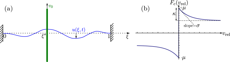
Figure V.1: (colour online) (a) Schematic of a bowed string. The bow is pulled with a constant velocity $v_{0}$, while the string exhibits a stick-slip vibration generated by the friction between the bow and the string. (b) Graph of the Coulomb-like friction force.

To see our theory applied to a mechanical system consider the example of a bowed string in Fig. V.1(a). We consider the same equation of motion as in section III.3, where we derived all the necessary ingredients of the reduced model apart from the contact force. Because $\boldsymbol{L}^{1}(\tau)$ has a discontinuity at $\tau=0$ this example falls into case 2. of section IV.

To complete the model we define the contact force $F_{c}$ of equation (IV.1) as the friction force between the bow and the string. We assume that the string is being bowed at $\xi=\xi^{\star}$ with velocity $v_{0}$ that generates the friction force

$$f_{c}(v_{\textrm{rel}})=\mathrm{sign}v_{\mathrm{rel}}\left(\mu-\kappa+\kappa\exp\left(-\sigma\left|v_{\mathrm{rel}}\right|\right)\right),$$ (V.1)

where $v_{\textrm{rel}}$ is the relative velocity of the string and the bow. The graph of the friction force function can be seen in Fig. V.1(b). In this example the static friction force is within the interval $[-\mu,\mu]$. The relative velocity between the string and the bow is expressed as a function of a resolved variable $v_{\mathrm{rel}}=y_{2}(t)-v_{0}$. We also use the relative velocity to define the switching surface $\Sigma$ by $h(\boldsymbol{y}(t))=v_{\mathrm{rel}}$. Therefore the contact force of equation (IV.1) becomes $F_{c}(\boldsymbol{y}(t))=f_{c}(h(\boldsymbol{y}(t)))$.

V.1 Numerical method

We use a simple explicit Euler method to approximate the solutions of (IV.1) and (IV.5). We assume that time is quantised in $\varepsilon$ chunks, so that $\boldsymbol{y}_{q}=\boldsymbol{y}(q\varepsilon)$, $f_{c,q}=f_{c}(q\varepsilon)$, where $q=0,1,2,\ldots$. In case of slipping the only unknown is the state variable $\boldsymbol{y}_{q}$ that is calculated using the formula

$$\boldsymbol{y}_{q+1}=\boldsymbol{y}_{q}+\varepsilon\Biggl{(}\boldsymbol{A}\boldsymbol{y}_{q}+\boldsymbol{L}^{\infty}f_{c,q}+\sum_{j=0}^{n}\boldsymbol{L}^{0}(j\varepsilon)\left(f_{c,q-j}-f_{c,q-j-1}\right)\\ +\boldsymbol{L}^{0}(q\varepsilon)f_{c,0}+\boldsymbol{H}(q\varepsilon)\boldsymbol{z}(0)\Biggr{)},$$ (V.2)

where the friction force $f_{c,q}=F_{c}\left(\left[\boldsymbol{y}_{q}\right]_{2}-v_{0}\right)$ is used. The integration is approximated by the rectangle rule. For just illustrating the theory such a crude approximation is sufficient while for better accuracy and efficiency higher order methods, such as the Runge-Kutta (Iserles, 1996) method could be used. In our calculations we keep the step size reasonably short at $\varepsilon=5\times 10^{-4}$.

If the relative velocity $h(\boldsymbol{y}_{q})=\left[\boldsymbol{y}_{q}\right]_{2}-v_{0}$ of the string and the bow becomes zero there are two possibilities. Either the trajectory crosses the switching surface $\Sigma$ or it will stay on $\Sigma$ satisfying the equation

$$\nabla h(\boldsymbol{y}_{q})\cdot(\boldsymbol{y}_{q+1}-\boldsymbol{y}_{q})=0,$$ (V.3)

that is, the discretised version of $h(\boldsymbol{y}(t))\cdot\dot{\boldsymbol{y}}(t)=0$. To test which case applies, we substitute (V.2) into (V.3) and solve for the friction force $f_{c,q}$ that would hold the string and the bow together, which becomes

$$f_{c,q}=\frac{-\nabla h(\boldsymbol{y}_{q})}{\nabla h(\boldsymbol{y}_{q})\cdot(\boldsymbol{L}^{\infty}+\boldsymbol{L}^{0}(0))}\Biggl{(}-\boldsymbol{L}^{0}(0)f_{c,q-1}+\boldsymbol{A}\boldsymbol{y}_{q}+\sum_{j=1}^{q}\boldsymbol{L}^{0}(j)\left(f_{c,q-j}-f_{c,q-j-1}\right)\\ +\boldsymbol{L}^{0}(q\varepsilon)f_{c,0}+\boldsymbol{H}(q\varepsilon)\boldsymbol{z}(0)\Biggr{)}.$$ (V.4)

If the calculated friction force satisfies $-\mu\leq f_{c,q}\leq\mu$, the bow and the string stick together. For the stick phase of motion we use equation (V.2) to advance the solution together with this dynamic friction force of equation (V.4).

V.2 Numerical results

To illustrate the properties of the dimension reduced equation (IV.1) we calculated a typical stick-slip trajectory starting at a the initial condition $\boldsymbol{z}(0)=y_{1}(0)\boldsymbol{w}_{1}+y_{2}(0)\boldsymbol{w}_{2}$ with $y_{1}(0)=-2.9224$ and $y_{2}(0)=-2.7668$. The parameters of the friction force in equation (V.1) are $\mu=4$, $\kappa=0.32$, $\sigma=1$, the speed of the bow is $v_{0}=\nicefrac{{3}}{{2}}$, the damping ratios are $D_{k}=\nicefrac{{1}}{{10}}$, $k=1,\ldots,N$ and the wave speed on the string is $c=1$. The string is bowed at $\xi^{\star}=0.4$.111The choice of these parameters was guided by the desire of producing stick-slip motion rather than physical consideration. We solved equation (II.3) using Matlab’s ode113 solver and (IV.1) using our method described in section V.1. The results of the the simulation for reduced and the full model shown in Figure V.2(a,b) are nearly indistinguishable, because the only approximations are within the numerical methods. The blue curves denote the solution of (IV.1) and the (almost invisible) red curve underneath represents the solution of (II.3) using solution techniques described by Piiroinen & Kuznetsov (2008).

Refer to caption
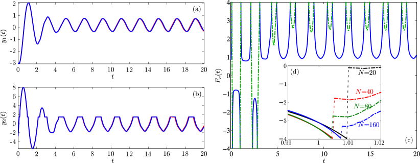
Figure V.2: Solution trajectories of equations (II.3) and (IV.1). (a) Displacement of the string and (b) velocity of the string at the contact point. (c) Friction force between the bow and string using equation (IV.1). The continuous lines denote slip, the dash-dotted lines represent sticking motion. (d) The discontinuity of the friction force at the onset of sticking disappears in the continuum limit. $N$ indicates the considered number of modes.

Initially the solution spends short time intervals on the switching surface and then settles into a periodic stick-slip motion. The stick phases can be recognised in Fig. V.2(b) as short horizontal sections at $y_{2}=1.5$. In Fig. V.2(c) the friction force is represented by the blue lines and the green dash-dotted lines for the slipping and the sticking motion, respectively. The friction force also appears to be discontinuous. To calculate this solution we did not use the converged $\boldsymbol{L}^{1}(\tau)$, instead we used a series of mode truncations shown in Fig. (III.2)(b). On a smaller scale Fig. V.2(d) shows that the gap in the friction force (dashed line) between the slipping segment (continuous line) and the sticking segment (dash dotted line) of the friction force vanishes as increasing number of modes of system (II.3) are considered. As the theory dictates the gap should vanish in the infinite dimensional case.

VI Conclusions

In this paper we considered vibrations of structures that are composed of linear elastic bodies coupled through strongly nonlinear contact forces such as friction. The coupling was assumed to occur at point contacts. We introduced an exact transformation based on the Mori-Zwanzig formalism that reduces the infinite dimensional system of ordinary differential equations to a description with time delay involving small number of variables. We found that the model reduction technique converges and contact forces become continuous even though the governing equation is discontinuous. We illustrated this novel technique through the example of a bowed string.

Through examples we found that if natural frequencies scale linearly with the mode number, the contact forces are Lipschitz continuous during the transition from slip to stick. This is the case of the elastic string. If the natural frequencies increase faster than linear, the contact forces are only continuous. The Euler-Bernoulli beam exhibits such a behaviour, but it also allows infinite wave speed, which can be though of as not physical. In reality however, every structure will have small scale longitudinal vibration components with linearly scaled frequencies similar to the Timoshenko beam model (Szalai, 2013). We expect that if all the details are considered for a linear structure, the contact forces must always be Lipschitz continuous in time. This finding together with the new form of governing equations could be used in further studies to understand the source of non-deterministic motion (Colombo & Jeffrey, 2011).

The reduced equations are also structurally stable. Small perturbations to the memory kernel or other terms only deform solutions but do not change their qualitative behaviour as long as the qualitative features of the memory kernel are preserved. This is a clear advantage over finite dimensional approximation of non-smooth systems, where small perturbations can cause qualitatively different solutions. Therefore once the qualitative form of the memory kernel is established non-smooth mechanical systems can be approximated more successfully using our description.

How non-smooth phenomena of low dimensional systems manifest in continuum structures is an open question. For low dimensional systems many singularities can occur that lead to chaotic and resonant vibration on invariant polygons (Szalai & Osinga, 2008), the Painleve paradox (Nordmark et al., 2011) and other types of discontinuity induced bifurcations. It remains to investigate how these phenomena occur in systems involving elastic structures and hence equations with memory.

Our theory is developed for linear structures coupled to strong nonlinearities. It is however possible to extend this framework to cases where the underlying structure is nonlinear. For the weakly nonlinear case the Hartman-Grobman theorem (Coddington & Levinson, 1955; Kuznetsov, 2004) guarantees the existence of a transformation that takes any weakly nonlinear system into a linear system about an equilibrium if that system is not undergoing a stability change. This generalisation is currently being worked on by the author.

We also assumed point contacts in our derivations. This is a significant simplification since most contact problems occur along a surface. The difficulty arises when one needs to deal with contacting surfaces that slip at one part of the contact surface while stick at others. An interesting question is if it is possible to develop a similar model reduction technique of such problems to involve only finite number of variables.

Acknowledgements

The author would like to thank Gábor Stépán, who brought his attention to the work of Chorin et al. (2000). He would also like thank Jan Sieber, Alan R. Champneys and John Hogan for useful discussion and comments on the manuscript.

Appendix A Model transformation

In this appendix we show that the infinite dimensional system (III.1) can be transformed into a finite dimensional delayed equation. The delay equation involves convolution integrals that can be related to Green’s functions, but only for part of the system. The procedure is based on the variation-of-parameters formula.

Consider the following linear forced system

$$\dot{\boldsymbol{z}}(t)=\boldsymbol{R}\boldsymbol{z}(t)+\boldsymbol{v}f(t),$$ (A.1)

where $\boldsymbol{z}(t),\boldsymbol{v}\in\mathbb{R}^{2N}$, $f(t)\in\mathbb{R}$ and $\boldsymbol{R}\in\mathbb{R}^{2N\times 2N}$. Assume matrices $\boldsymbol{V}\in\mathbb{R}^{2M\times 2N}$ and $\boldsymbol{W}\in\mathbb{R}^{2N\times 2M}$ such that $\boldsymbol{S}=\boldsymbol{W}\boldsymbol{V}$ is a projection matrix $\boldsymbol{S}=\boldsymbol{S}^{2}$ with a $2M$ dimensional range. $\boldsymbol{S}$ is a projection if and only if $\boldsymbol{V}\boldsymbol{W}=\boldsymbol{I}_{2M}$, where $\boldsymbol{I}_{2M}$ is the $2M$ dimensional identity. Also, define the complementary projection matrix $\boldsymbol{Q}=\boldsymbol{I}-\boldsymbol{S}$ and the resolved coordinates $\boldsymbol{y}(t)=\boldsymbol{V}\boldsymbol{z}(t)$. With this notation we rewrite equation (A.1) into

$$\dot{\boldsymbol{z}}(t)=\boldsymbol{R}\boldsymbol{S}\boldsymbol{z}(t)+\boldsymbol{R}\boldsymbol{Q}\boldsymbol{z}(t)+\boldsymbol{v}f(t).$$ (A.2)

Assume that the solution of $\dot{\boldsymbol{z}}(t)=\boldsymbol{R}\boldsymbol{Q}\boldsymbol{z}(t)$ can be computed for specific initial conditions. Therefore the solution of (A.2) can formally be expressed using the variation-of-parameters or Dyson’s (Coddington & Levinson, 1955) formula as

$$\boldsymbol{z}(t)=\mathrm{e}^{\boldsymbol{R}\boldsymbol{Q}(t-s)}\boldsymbol{z}(s)+\int_{0}^{t-s}\mathrm{e}^{\boldsymbol{R}\boldsymbol{Q}\tau}\left(\boldsymbol{R}\boldsymbol{S}\boldsymbol{z}(t-\tau)+\boldsymbol{v}f(t-\tau)\right)\mathrm{d}\tau.$$ (A.3)

Substituting this result into the second term on the right side of (A.2) we get

$$\dot{\boldsymbol{z}}(t)=\boldsymbol{R}\boldsymbol{S}\boldsymbol{z}(t)+\boldsymbol{v}f(t)\\ +\boldsymbol{R}\boldsymbol{Q}\left\{\mathrm{e}^{\boldsymbol{R}\boldsymbol{Q}(t-s)}\boldsymbol{z}(s)+\int_{0}^{t-s}\mathrm{e}^{\boldsymbol{R}\boldsymbol{Q}\tau}\left(\boldsymbol{R}\boldsymbol{S}\boldsymbol{z}(t-\tau)+\boldsymbol{v}f(t-\tau)\right)\right\}\mathrm{d}\tau.$$ (A.4)

Note that $\boldsymbol{S}\boldsymbol{z}(t)=\boldsymbol{W}\boldsymbol{V}\boldsymbol{z}(t)=\boldsymbol{W}\boldsymbol{y}(t)$ and project (A.4) using $\boldsymbol{V}$, to get

$$\dot{\boldsymbol{y}}(t)=\boldsymbol{V}\boldsymbol{R}\boldsymbol{W}\boldsymbol{y}(t)+\boldsymbol{V}\boldsymbol{v}f(t)\\ +\boldsymbol{V}\boldsymbol{R}\boldsymbol{Q}\left\{\mathrm{e}^{\boldsymbol{R}\boldsymbol{Q}(t-s)}\boldsymbol{z}(s)+\int_{0}^{t-s}\mathrm{e}^{\boldsymbol{R}\boldsymbol{Q}\tau}\left(\boldsymbol{R}\boldsymbol{S}\boldsymbol{z}(t-\tau)+\boldsymbol{v}f(t-\tau)\right)\right\}\mathrm{d}\tau,$$ (A.5)

which is the reduced equation for only the resolved coordinates $\boldsymbol{y}(t)$. Note that $\boldsymbol{R}\boldsymbol{Q}\mathrm{e}^{\boldsymbol{R}\boldsymbol{Q}\tau}=\nicefrac{{d}}{{d\tau}}\mathrm{e}^{\boldsymbol{R}\boldsymbol{Q}\tau}$ hence the integrals can be rewritten with Riemann-Stieltjes integrals as

$$\dot{\boldsymbol{y}}(t)=\boldsymbol{A}\boldsymbol{y}(t)+\int_{0}^{t-s}\mathrm{d}_{\tau}\boldsymbol{K}(\tau)\boldsymbol{y}(t-\tau)+\int_{0}^{t-s}\mathrm{d}_{\tau}\boldsymbol{L}(\tau)f(t-\tau)+\boldsymbol{V}\boldsymbol{v}f(t)+\boldsymbol{H}(t)\boldsymbol{z}(s),$$ (A.6)

where

$\displaystyle\boldsymbol{A}$ $\displaystyle=\boldsymbol{V}\boldsymbol{R}\boldsymbol{W},$ $\displaystyle\in\mathbb{R}^{2M\times 2M}$ (A.7)
$\displaystyle\boldsymbol{H}(t)\boldsymbol{z}(s)$ $\displaystyle=\boldsymbol{V}\boldsymbol{R}\boldsymbol{Q}\mathrm{e}^{\boldsymbol{R}\boldsymbol{Q}(t-s)}\boldsymbol{z}(s),$ $\displaystyle\in\mathbb{R}^{2M}$ (A.8)
$\displaystyle\boldsymbol{K}(\tau)$ $\displaystyle=\boldsymbol{V}\mathrm{e}^{\boldsymbol{R}\boldsymbol{Q}\tau}\boldsymbol{R}\boldsymbol{W},$ $\displaystyle\in\mathbb{R}^{2M\times 2M}$ (A.9)
$\displaystyle\boldsymbol{L}(\tau)$ $\displaystyle=\boldsymbol{V}\mathrm{e}^{\boldsymbol{R}\boldsymbol{Q}\tau}\boldsymbol{v}.$ $\displaystyle\in\mathbb{R}^{2M}$ (A.10)

If the range of $\boldsymbol{W}$ is invariant under $\boldsymbol{R}$, then $\boldsymbol{K}(\tau)=\boldsymbol{A}$ constant. This occurs because the image of the range of $\boldsymbol{W}$ is in the kernel of $\boldsymbol{Q}$. Consequently the integral with $\boldsymbol{K}(\tau)$ vanishes.

Note that this procedure is a simplified version of the Mori-Zwanzig formalism (Chorin et al., 2000; Evans & Morriss, 2008) for linear systems. Therefore our procedure can be extended to nonlinear systems. In the nonlinear case $\boldsymbol{A}\boldsymbol{y}$, $\boldsymbol{K}(\tau)\boldsymbol{y}$ and $\boldsymbol{L}(\tau)f$ become nonlinear functions of $\boldsymbol{y}$ and $f$, respectively.

Appendix B The memory kernels

In this appendix we show that the memory kernel can be obtained from the solution of the first order system (III.1) if condition (III.5) holds. Condition (III.5) implies that there is a $2M\times 2M$ matrix $\boldsymbol{X}$ such that $\boldsymbol{R}\boldsymbol{W}=\boldsymbol{W}\boldsymbol{X}$. If we multiply this expression by $\boldsymbol{V}$ from the left we get the identity $\boldsymbol{A}=\boldsymbol{V}\boldsymbol{R}\boldsymbol{W}=\boldsymbol{V}\boldsymbol{W}\boldsymbol{X}=\boldsymbol{X}$. As a consequence for any integer $p$ we must have

$$\boldsymbol{R}^{p}\boldsymbol{W}=\boldsymbol{W}\boldsymbol{A}^{p}.$$ (B.1)

To investigate the expression $\mathrm{e}^{\boldsymbol{R}\boldsymbol{Q}t}$ that occurs in the definition of the memory kernel (A.10) we define

$$\boldsymbol{\varPhi}(t)=\mathrm{e}^{\boldsymbol{R}\boldsymbol{Q}t}\mathrm{e}^{-\boldsymbol{R}t}$$ (B.2)

so that $\mathrm{e}^{\boldsymbol{R}\boldsymbol{Q}t}=\boldsymbol{\varPhi}(t)\mathrm{e}^{\boldsymbol{R}t}$. The power series expansion of $\boldsymbol{\varPhi}(t)$ can be written as $\boldsymbol{\varPhi}(t)=\sum_{n=0}^{\infty}\frac{t^{n}}{n!}\left.\frac{\mathrm{d}^{n}}{\mathrm{d}t^{n}}\boldsymbol{\varPhi}(t)\right|_{t=0}$. The derivatives are calculated as

$\displaystyle\left.\frac{\mathrm{d}^{n}}{\mathrm{d}t^{n}}\boldsymbol{\varPhi}(t)\right|_{t=0}$ $\displaystyle=\sum_{k=0}^{n}\binom{n}{k}\left(\boldsymbol{R}-\boldsymbol{R}\boldsymbol{S}\right)^{k}\left(-\boldsymbol{R}\right)^{n-k}$
$\displaystyle=\sum_{k=0}^{n}\binom{n}{k}\sum_{p_{i}+q_{i}=1}\boldsymbol{R}^{p_{1}}\left(-\boldsymbol{R}\boldsymbol{S}\right)^{q_{1}}\cdots\boldsymbol{R}^{p_{k}}\left(-\boldsymbol{R}\boldsymbol{S}\right)^{q_{k}}\left(-\boldsymbol{R}\right)^{n-k}.$ (B.3)

We can transform the products in (B.3) to simpler expressions. Assume that in the second summation for a fixed $r\in\{0,\ldots,k\}$, $q_{r}=1$ and $q_{i}=0$ if $i>r$, while the rest of $q_{i}$ are arbitrary. The sets of $p_{i},q_{i}$ are disjoint for different $r$ values and their union covers all possible $p_{i},q_{i}$ values once. Using formula (B.1) and $\boldsymbol{R}\boldsymbol{S}=\boldsymbol{W}\boldsymbol{A}\boldsymbol{V}$ we find that

$$\boldsymbol{R}^{p_{1}}\left(-\boldsymbol{R}\boldsymbol{S}\right)^{q_{1}}\cdots\boldsymbol{R}^{p_{k}}\left(-\boldsymbol{R}\boldsymbol{S}\right)^{q_{k}}=(-1)^{\sum q_{i}}\boldsymbol{W}\boldsymbol{A}^{r}\boldsymbol{V}\boldsymbol{R}^{k-r}.$$ (B.4)

The sum of all terms corresponding to each $r\neq$0 can be written as

$$\sum_{l=0}^{r-1}\binom{r-1}{l}(-1)^{l+1}\boldsymbol{W}\boldsymbol{A}^{r}\boldsymbol{V}\boldsymbol{R}^{k-r}=\begin{cases}-\boldsymbol{W}\boldsymbol{A}\boldsymbol{V}\boldsymbol{R}^{k-1}&\mbox{if}\;r=1\\ 0&\mbox{if}\;r>1\end{cases}.$$ (B.5)

For $r=0$, the sum is $\boldsymbol{R}^{k}$. Therefore the $n$-th derivative for $n>0$ reads

$\displaystyle\left.\frac{\mathrm{d}^{n}}{\mathrm{d}t^{n}}\boldsymbol{\varPhi}(t)\right|_{t=0}$ $\displaystyle=\left(-\boldsymbol{R}\right)^{n}+\sum_{k=1}^{n}\binom{n}{k}\left(\boldsymbol{R}^{k}-\boldsymbol{W}\boldsymbol{A}\boldsymbol{V}\boldsymbol{R}^{k-1}\right)\left(-\boldsymbol{R}\right)^{n-k}$ (B.6)
$\displaystyle=\sum_{k=0}^{n}\binom{n}{k}\boldsymbol{R}^{k}\left(-\boldsymbol{R}\right)^{n-k}-\sum_{k=1}^{n}\binom{n}{k}\boldsymbol{W}\boldsymbol{A}\boldsymbol{V}\boldsymbol{R}^{k-1}\left(-\boldsymbol{R}\right)^{n-k}$ (B.7)
$\displaystyle=(-1)^{n}\boldsymbol{W}\boldsymbol{A}\boldsymbol{V}\boldsymbol{R}^{n-1}.$ (B.8)

Substituting the derivatives into the power series we are left with

$$\boldsymbol{\varPhi}(t)=\boldsymbol{I}-\sum_{n=1}^{\infty}\frac{t^{n}}{n!}(-1)^{n-1}\boldsymbol{W}\boldsymbol{A}\boldsymbol{V}\boldsymbol{R}^{n-1}=\boldsymbol{I}-\boldsymbol{W}\boldsymbol{A}\boldsymbol{V}\int_{0}^{t}\mathrm{e}^{-\boldsymbol{R}\tau}\mathrm{d}\tau.$$ (B.9)

Multiplying $\boldsymbol{\varPhi}(t)$ from the right by $\mathrm{e}^{\boldsymbol{R}t}$ we get the formula

$$\mathrm{e}^{\boldsymbol{R}\boldsymbol{Q}t}=\mathrm{e}^{\boldsymbol{R}t}-\boldsymbol{R}\boldsymbol{S}\int_{0}^{t}\mathrm{e}^{\boldsymbol{R}(t-\tau)}\mathrm{d}\tau=\mathrm{e}^{\boldsymbol{R}t}-\boldsymbol{R}\boldsymbol{S}\int_{0}^{t}\mathrm{e}^{\boldsymbol{R}\tau}\mathrm{d}\tau.$$ (B.10)

With this result the forcing term and the memory kernels become

$$\displaystyle\boldsymbol{H}(t)\boldsymbol{z}(s)=\boldsymbol{V}\boldsymbol{R}\boldsymbol{Q}\mathrm{e}^{\boldsymbol{R}(t-s)}\boldsymbol{z}(s),\;\boldsymbol{K}(\tau)=\boldsymbol{A},\;\boldsymbol{L}(\tau)=\left(\boldsymbol{V}\mathrm{e}^{\boldsymbol{R}\tau}-\boldsymbol{A}\boldsymbol{V}\int_{0}^{\tau}\mathrm{e}^{\boldsymbol{R}\theta}\mathrm{d}\theta\right)\boldsymbol{v}.$$

Appendix C Strong continuity of $\mathrm{e}^{\boldsymbol{R}t}$

In order to justify our analysis we need to show that $\mathrm{e}^{\boldsymbol{R}t}$ is a strongly continuous semigroup. We use the Hille-Yosida theorem (Pazy, 1983; Hille & Phillips, 1957), which states that $\mathrm{e}^{\boldsymbol{R}t}$ is a strongly continuous semigroup satisfying $\left\|\mathrm{e}^{\boldsymbol{R}t}\right\|\leq M_{0}$ if and only if $\overline{\mathcal{D}(\boldsymbol{R})}=\boldsymbol{Z}$ and

$$\left\|(\boldsymbol{R}-\lambda\boldsymbol{I})^{-n}\right\|\leq M_{0}\lambda^{-n}$$ (C.1)

for $\lambda>0$ and $n=1,2,3,\ldots$, where $\boldsymbol{Z}$ is defined by equation (III.32).

First we show that if $\boldsymbol{R}$ satisfies (III.33) and that each eigenvalue of $\boldsymbol{R}$ has finite multiplicity then condition (C.1) is satisfied. Using a linear transformation matrix $\boldsymbol{R}$ can be brought into its block diagonal Jordan normal form. Each block in the diagonal of the Jordan normal form corresponds to an eigenvalue $\lambda_{k}$ of $\boldsymbol{R}$ and has size $l_{k}$. The form of such a block is

$$\boldsymbol{J}_{k}=\left(\begin{array}[]{cccc}\lambda_{k}&1&0&0\\ 0&\lambda_{k}&\ddots&0\\ 0&\ddots&\ddots&1\\ 0&0&0&\lambda_{k}\end{array}\right).$$ (C.2)

After inversion the component of $(\boldsymbol{R}-\lambda\boldsymbol{I})^{-n}$ that corresponds to $J_{k}$ becomes

$$\left(\boldsymbol{J}_{k}-\lambda\boldsymbol{I}\right)^{-n}=\left(\begin{array}[]{cccc}\left(\lambda_{k}-\lambda\right)^{-n}&-n\left(\lambda_{k}-\lambda\right)^{-n-1}&\cdots&(-1)^{l}\binom{n+l_{k}-1}{l_{k}}\left(\lambda_{k}-\lambda\right)^{-n-l_{k}}\\ 0&\left(\lambda_{k}-\lambda\right)^{-n}&\ddots&\vdots\\ 0&0&\ddots&-n\left(\lambda_{k}-\lambda\right)^{-n-1}\\ 0&0&0&\left(\lambda_{k}-\lambda\right)^{-n}\end{array}\right).$$ (C.3)

The norm of this Jordan block can be estimated by

$$\left\|\left(\boldsymbol{J}_{k}-\lambda\boldsymbol{I}\right)^{-n}\right\|\leq\left|\lambda_{k}-\lambda\right|^{-n}+n\left|\lambda_{k}-\lambda\right|^{-n-1}+\cdots+\binom{n+l_{k}-1}{l_{k}}\left|\lambda_{k}-\lambda\right|^{-n-l_{k}}.$$ (C.4)

Note that $\left|\lambda_{k}-\lambda\right|\geq\left|\Re\lambda_{k}-\lambda\right|$. Since $\lambda>0\geq\Re\lambda_{k}$ one can find an $M_{k}$ such that

$$\left\|\left(\boldsymbol{J}_{k}-\lambda\boldsymbol{I}\right)^{-n}\right\|\leq M_{k}\lambda^{-n}$$ (C.5)

Considering this estimate for all Jordan blocks we find that

$$\left\|(\boldsymbol{R}-\lambda\boldsymbol{I})^{-n}\right\|\leq\sup_{k}M_{k}\lambda^{-n}\leq M_{0}\lambda^{-n},$$ (C.6)

where $M_{0}=\sup_{k}M_{k}$. This proves (C.1).

To conclude the proof we show that $\overline{\mathcal{D}(\boldsymbol{R})}=\boldsymbol{Z}$. Again, we use the Jordan normal form. We partition every vector in $\boldsymbol{Z}$ such that $\boldsymbol{z}=(\boldsymbol{z}_{1},\boldsymbol{z}_{2},\ldots)^{T}$, where $\boldsymbol{z}_{k}$ are of the size of a Jordan block. Let $\boldsymbol{z}\in\boldsymbol{Z}$ and construct $\boldsymbol{z}^{P}=(\boldsymbol{z}_{1},\boldsymbol{z}_{2},\ldots,\boldsymbol{z}_{P},0,\ldots)^{T}$ such that it has $P$ number of non-zero components. This guarantees that for any $\boldsymbol{z}^{P}$, $\left\|\boldsymbol{R}\boldsymbol{z}^{P}\right\|<\infty$, hence $\boldsymbol{z}^{P}\in\mathcal{D}(\boldsymbol{R})$. It is also clear that $\left\|\lim_{P\to\infty}\boldsymbol{z}_{P}\right\|<\infty$ due to its construction, thus we have shown that $\overline{\mathcal{D}(\boldsymbol{R})}=\boldsymbol{X}$.

Appendix D Boundedness and smoothness of $\boldsymbol{L}_{j}^{1}(\tau)$

The definition (III.18) with (III.13) of $\boldsymbol{L}_{j}^{1}(\tau)$ has two terms both including the expression $\boldsymbol{\Upsilon}_{j}(\tau)=\boldsymbol{V}\int_{0}^{\tau}\mathrm{e}^{\boldsymbol{R}\theta}\boldsymbol{v}_{M+j}\mathrm{d\theta}$. Therefore we only need to consider $\boldsymbol{\Upsilon}_{j}(\tau)$ in our analysis to show boundedness and smoothness of $\boldsymbol{L}_{j}^{1}(\tau)$.

We use the inverse Laplace transform (Pazy, 1983) to obtain

$$\mathrm{e}^{\boldsymbol{R}\tau}\boldsymbol{x}=\frac{1}{2\pi i}\int_{\Gamma_{0}}\mathrm{e}^{\lambda\tau}\left(\lambda\boldsymbol{I}-\boldsymbol{R}\right)^{-1}\boldsymbol{x}\mathrm{d}\lambda,$$ (D.1)

where $\Gamma_{0}=\{\lambda\in\mathbb{C}:\Re\lambda=\gamma>0\}$. Using integration rules for the Laplace transform and multiplying (D.1) by vectors $\boldsymbol{v}_{M+j}$ and $\boldsymbol{v}_{\ell}$ from the left and right, respectively, we get

$$\left[\boldsymbol{\Upsilon}_{j}(\tau)\right]_{\ell}=\frac{1}{2\pi i}\int_{\Gamma_{0}}\mathrm{e}^{\lambda\tau}\boldsymbol{v}_{\ell}\cdot\left(\lambda\boldsymbol{I}-\boldsymbol{R}\right)^{-1}\boldsymbol{v}_{M+j}\frac{\mathrm{d}\lambda}{\lambda},$$ (D.2)

The equality makes sense if the integral converges. Evaluating the inverse operator in (D.2) we find that

$$\left(\lambda\boldsymbol{I}-\boldsymbol{R}\right)^{-1}\left(\begin{array}[]{c}\boldsymbol{0}\\ \boldsymbol{n}_{j}\end{array}\right)=\left(\begin{array}[]{c}-(\boldsymbol{K}+\lambda\boldsymbol{C}+\lambda^{2})^{-1}\boldsymbol{n}_{j}\\ -\lambda(\boldsymbol{K}+\lambda\boldsymbol{C}+\lambda^{2})^{-1}\boldsymbol{n}_{j}\end{array}\right).$$ (D.3)

Note that it is sufficient to consider $\left[\boldsymbol{\Upsilon}_{j}(\tau)\right]_{M+l}$ since $\left[\boldsymbol{\Upsilon}_{j}(\tau)\right]_{l}$ is the integral of $\left[\boldsymbol{\Upsilon}_{j}(\tau)\right]_{M+l}$. Substituting (D.3) into (D.2) we are left with

$\displaystyle\left[\boldsymbol{\Upsilon}_{j}(\tau)\right]_{M+l}$ $\displaystyle=\frac{1}{2\pi i}\int_{\Gamma_{0}}\mathrm{e}^{\lambda\tau}\boldsymbol{n}_{l}\cdot(\boldsymbol{K}+\lambda\boldsymbol{C}+\lambda^{2})^{-1}\boldsymbol{n}_{j}\mathrm{d}\lambda.$ (D.4)

The integral of the inverse Laplace transform (D.2) converges for all $t\geq 0$ if

$$\left|\lambda\boldsymbol{n}_{l}\cdot(\boldsymbol{K}+\lambda\boldsymbol{C}+\lambda^{2})^{-1}\boldsymbol{n}_{j}\right|\leq M_{j,l}\;\mbox{for}\;\lambda\in\Gamma_{0}$$ (D.5)

and for $j,l=1,\ldots,M$. Indeed, by estimating the bound we get

$$\left|\int_{0}^{\tau}\left[\boldsymbol{\Upsilon}_{j}(\tau)\right]_{M+l}\right|\leq\frac{1}{2\pi i}M_{j,l}\left|\int_{\Gamma_{0}}\mathrm{e}^{\lambda\tau}\frac{\mathrm{d}\lambda}{\lambda}\right|=M_{j,l}.$$ (D.6)

This implies that $\boldsymbol{L}_{j}^{1}$ is bounded.

If the stronger conditions (III.35) and (III.36) are satisfied, we can alter the contour of integration so that it is within the left half of the complex plane, $\Gamma_{\delta}=\{\lambda\in\mathbb{C}:\left|\arg\lambda\right|=\nicefrac{{\pi}}{{2}}+\delta\}$, where $\delta>0$ is sufficiently small so that all the eigenvalues of $\boldsymbol{R}$ are on the left of $\Gamma_{\delta}$. We parametrise the contour $\Gamma_{\delta}$ by $\lambda=\kappa\mathrm{e}^{\pm i(\nicefrac{{\pi}}{{2}}+\delta)}$, $\kappa\geq 0$. Using this contour we find that the derivative

$$\left[\boldsymbol{\Upsilon}_{j}(\tau)\right]_{M+l}=\frac{1}{2\pi i}\int_{\Gamma_{\delta}}\mathrm{e}^{\lambda\tau}\lambda\boldsymbol{n}_{l}\cdot(\boldsymbol{K}+\lambda\boldsymbol{C}+\lambda^{2})^{-1}\boldsymbol{n}_{j}\mathrm{d}\lambda$$ (D.7)

can be estimated by

$$\left|\left[\boldsymbol{\Upsilon}_{j}(\tau)\right]_{M+l}\right|\leq\frac{1}{\pi}\int_{0}^{\infty}M_{j,l}\mathrm{e}^{-\kappa\tau\cos 2\delta}\mathrm{d}\kappa=\frac{1}{\tau}\left(\frac{M_{j,l}}{\pi\cos 2\delta}\right).$$ (D.8)

This means that the derivative of $\boldsymbol{L}_{j}^{1}$ is also bounded but only for $\tau>0$. Due to $\mathrm{e}^{\boldsymbol{R}\tau}$ being a strongly continuous semigroup (Theorem 2.5.2 in Pazy (1983)) higher derivatives are also bounded

$$\frac{1}{n!}\frac{\mathrm{d}^{n-1}}{\mathrm{d}\tau^{n-1}}\left|\left[\boldsymbol{\Upsilon}_{j}(\tau)\right]_{M+l}\right|\leq\left(\frac{C_{j,l}\mathrm{e}}{\tau}\right)^{n},$$ (D.9)

for $C_{j,l}<\infty$ which proves that $\boldsymbol{L}_{j}^{1}$ is smooth for $\tau>0$.

Appendix E Discontinuity of the memory kernel of the pre-tensed string

Here we show that the memory kernel $\boldsymbol{L}^{1}(\tau)$ of the bowed string is discontinuous at $\tau=0$. In equation (III.29) the terms that cause discontinuity are divided by the lowest power of $\omega_{k}$. The other terms are continuous and add up to zero at $\tau=0$. Therefore, after using $D_{k}=D$ and $\omega_{k}=ck\pi$ the following identity holds:

$$\lim_{\tau\to 0+}\left[\boldsymbol{L}^{1}(\tau)\right]_{2}=\lim_{\tau\to 0+}\sum_{k=1}^{\infty}\kappa_{k}(\tau),\;\kappa_{k}(\tau)=\frac{e^{-k\pi cD\tau}\sin^{2}k\pi\xi^{\star}}{k\pi c\sqrt{1-D^{2}}}\sin\left(k\pi c\sqrt{1-D^{2}}\tau\right).$$ (E.1)

One can expand $\kappa_{k}(\tau)$ in (E.1) as a sum of exponentials

$$\kappa_{k}(\tau)=\frac{1}{4k\pi c\sqrt{D^{2}-1}}\biggl{(}\mathrm{e}^{k\pi c\left(\sqrt{D^{2}-1}-D\right)\tau}-\mathrm{e}^{-k\pi c\left(\sqrt{D^{2}-1}+D\right)\tau}+\frac{1}{2}\mathrm{e}^{-k\pi\left(c\left(\sqrt{D^{2}-1}+D\right)\tau+2i\zeta\right)}\\ -\frac{1}{2}\mathrm{e}^{k\pi\left(c\left(\sqrt{D^{2}-1}-D\right)\tau-2i\zeta\right)}+\frac{1}{2}\mathrm{e}^{-k\pi\left(c\left(\sqrt{D^{2}-1}+D\right)\tau-2i\zeta\right)}-\frac{1}{2}\mathrm{e}^{k\pi\left(c\left(\sqrt{D^{2}-1}-D\right)\tau+2i\zeta\right)}\biggr{)}.$$ (E.2)

Since $\sum_{k=1}^{\infty}\frac{\mathrm{e}^{ka}}{k}=-\log(1-\mathrm{e}^{a})$, the limit (E.1) can be written as

$$\lim_{\tau\to 0+}\left[\boldsymbol{L}^{1}(\tau)\right]_{2}=\lim_{\tau\to 0+}\frac{-1}{4\pi c\sqrt{D^{2}-1}}\left\{\log(1-\mathrm{e}^{a_{1}})-\log(1-\mathrm{e}^{a_{2}})+\frac{1}{2}\sum_{l=3}^{6}(-1)^{l+1}\log(1-\mathrm{e}^{a_{l}})\right\},$$ (E.3)

where

$\displaystyle a_{1}=\pi c\left(\sqrt{D^{2}-1}-D\right)\tau,$ $\displaystyle a_{2}=-\pi c\left(\sqrt{D^{2}-1}+D\right)\tau,$ (E.4)
$\displaystyle a_{3,4}=\mp\pi\left(c\left(\sqrt{D^{2}-1}+D\right)\tau+2i\zeta\right),$ $\displaystyle a_{5,6}=\mp\pi\left(c\left(\sqrt{D^{2}-1}+D\right)\tau-2i\zeta\right),$ (E.5)

Discontinuity occurs if the path of $1-\mathrm{e}^{a_{l}(\tau)}$ crosses the non-positive real axis (including zero) at $\tau=0$. This is possible for $a_{1}$ and $a_{2}$ only if $0<\xi<1$, $\xi\neq\nicefrac{{1}}{{2}}$. Since we are taking a limit, it is sufficient to use a first order approximation at $\tau=0$, that is, $1-\mathrm{e}^{a_{l}(\tau)}\approx-a_{l}(\tau)$. Also note that $\log x=\log\left|x\right|+i\arg x$ and that $\left|a_{1}\right|=\left|a_{2}\right|=\pi c\tau$. The limit therefore becomes

$$\lim_{\tau\to 0+}\left[\boldsymbol{L}^{1}(\tau)\right]_{2}=\frac{-1}{4\pi c\sqrt{1-D^{2}}}\left(\arg\left(\sqrt{D^{2}-1}-D\right)-\arg\left(-\sqrt{D^{2}-1}-D\right)\right).$$ (E.6)

Assuming that $D=\cos\phi$, $0\leq\phi\leq\nicefrac{{\pi}}{{2}}$, we get $\arg\left(\sqrt{D^{2}-1}-D\right)=\pi-\phi$ and $\arg\left(-\sqrt{D^{2}-1}-D\right)=\pi+\phi$, hence

$$\lim_{\tau\to 0+}\left[\boldsymbol{L}^{1}(t)\right]_{2}=\frac{\cos^{-1}D}{2\pi c\sqrt{1-D^{2}}}.$$ (E.7)

References

  • Abramowitz & Stegun (1964) Abramowitz, M. & Stegun, I. 1964 Handbook of mathematical functions. New York: Dover, 5th edn.
  • Chorin et al. (2000) Chorin, A. J., Hald, O. H. & Kupferman, R. 2000 Optimal prediction and the mori-zwanzig representation of irreversible processes. Proc. Natl. Acad. Sci. U. S. A., 97(7), 2968–2973.
  • Coddington & Levinson (1955) Coddington, E. & Levinson, N. 1955 Theory of ordinary differential equations. McGraw-Hill.
  • Colombo & Jeffrey (2011) Colombo, A. & Jeffrey, M. 2011 Nondeterministic chaos, and the two-fold singularity in piecewise smooth flows. SIAM Journal on Applied Dynamical Systems, 10(2), 423–451.
  • di Bernardo et al. (2008) di Bernardo, M., Budd, C., Champneys, A. R. & Kowalczyk, P. 2008 Piecewise-smooth dynamical systems: Theory and applications. Springer.
  • Evans & Morriss (2008) Evans, D. J. & Morriss, G. 2008 Statistical mechanics of nonequilibrium liquids. Cambridge University Press, 2nd edn.
  • Ewins (2000) Ewins, D. J. 2000 Modal testing: Theory, practice and application (mechanical engineering research studies: Engineering dynamics series). Wiley-Blackwell.
  • Farkas & Stépán (1992) Farkas, M. & Stépán, G. 1992 On perturbation of the kernel in infinite delay systems. ZAMM, 72(1), 153–156.
  • Filippov & Arscott (2010) Filippov, A. & Arscott, F. 2010 Differential equations with discontinuous righthand sides: Control systems. Mathematics and its Applications. Springer.
  • Firrone (2009) Firrone, C. M. 2009 Measurement of the kinematics of two underplatform dampers with different geometry and comparison with numerical simulation. J. Sound Vibr., 323(1-2), 313–333.
  • Hale & Lunel (1993) Hale, J. & Lunel, S. 1993 Introduction to functional differential equations. No. v. 99 in Applied Mathematical Sciences. Springer.
  • Hess & Soom (1990) Hess, D. P. & Soom, A. 1990 Friction at a lubricated line contact operating at oscillating sliding velocities. Journal of Tribology - Transactions of the ASME, 112(1), 147–152.
  • Hille & Phillips (1957) Hille, E. & Phillips, R. S. 1957 Functional analysis and semi-groups. Colloquium Publications, 31. Providence.
  • Iserles (1996) Iserles, A. 1996 A first course in the numerical analysis of differential equations. Cambridge University Press.
  • Kuznetsov (2004) Kuznetsov, Y. 2004 Elements of applied bifurcation theory. Springer-Verlag, 3rd edn.
  • McBride (1979) McBride, A. 1979 Fractional calculus and integral transforms of generalized functions. Research notes in mathematics. Pitman Advanced Publishing Program.
  • Melcher et al. (2013) Melcher, J., Champneys, A. R. & Wagg, D. J. 2013 The impacting cantilever: modal non-convergence and the importance of stiffness matching. Philosophical Transactions of the Royal Society A: Mathematical, Physical and Engineering Sciences, 371, 20120 434.
  • Nordmark et al. (2011) Nordmark, A., Dankowicz, H. & Champneys, A. R. 2011 Friction-induced reverse chatter in rigid-body mechanisms with impacts. IMA J. Appl. Math., 76, 85–119.
  • Oestreich et al. (1997) Oestreich, M., Hinrichs, N. & Popp, K. 1997 Dynamics of oscillators with impact and friction. Chaos, Solitons & Fractals, 8(4), 535–558.
  • Pacejka & Besselink (1997) Pacejka, H. & Besselink, I. 1997 Magic formula tyre model with transient properties. Vehicle System Dynamics: International Journal of Vehicle Mechanics and Mobility, 27(S1), 234–249.
  • Pazy (1983) Pazy, A. 1983 Semigroups of linear operators and applications to partial differential equations, vol. 44 of Applied Mathematical Sciences. New York: Springer-Verlag.
  • Petrov (2008) Petrov, E. P. 2008 Explicit finite element models of friction dampers in forced response analysis of bladed disks. J. Eng. Gas. Turbines Power-Trans. ASME, 130(2).
  • Piiroinen & Kuznetsov (2008) Piiroinen, P. T. & Kuznetsov, Y. A. 2008 An event-driven method to simulate Filippov systems with accurate computing of sliding motions. ACM Trans. Math. Softw., 34(3), 13:1–13:24.
  • Putelat et al. (2011) Putelat, T., Dawes, J. H. P. & Willis, J. R. 2011 On the microphysical foundations of rate-and-state friction. J. Mech. Phys. Solids, 59(5), 1062–1075.
  • Quinn (2012) Quinn, D. D. 2012 Modal analysis of jointed structures. Journal of Sound and Vibration, 331(1), 81–93.
  • Segalman (2006) Segalman, D. J. 2006 Modelling joint friction in structural dynamics. Structural Control and Health Monitoring, 13(1), 430–453.
  • Sieber & Kowalczyk (2010) Sieber, J. & Kowalczyk, P. 2010 Small-scale instabilities in dynamical systems with sliding. Physica D, 239(1-2), 44–57.
  • Stépán & Szabó (1999) Stépán, G. & Szabó, Z. 1999 Impact induced internal fatigue cracks. In Proceedings of the detc’99.
  • Szalai (2013) Szalai, R. 2013 arXiv:1306.2224 [math.DS] Impact mechanics of elastic bodies with point contact. submitted.
  • Szalai & Osinga (2008) Szalai, R. & Osinga, H. M. 2008 Invariant polygons in systems with grazing-sliding. Chaos: An Interdisciplinary Journal of Nonlinear Science, 18(2), 023 121.