Discriminative Extended Canonical Correlation Analysis for Pattern Set Matching

Abstract

In this paper we address the problem of matching sets of vectors embedded in the same input space. We propose an approach which is motivated by canonical correlation analysis (CCA), a statistical technique which has proven successful in a wide variety of pattern recognition problems. Like CCA when applied to the matching of sets, our extended canonical correlation analysis (E-CCA) aims to extract the most similar modes of variability within two sets. Our first major contribution is the formulation of a principled framework for robust inference of such modes from data in the presence of uncertainty associated with noise and sampling randomness. E-CCA retains the efficiency and closed form computability of CCA, but unlike it, does not possess free parameters which cannot be inferred directly from data (inherent data dimensionality, and the number of canonical correlations used for set similarity computation). Our second major contribution is to show that in contrast to CCA, E-CCA is readily adapted to match sets in a discriminative learning scheme which we call discriminative extended canonical correlation analysis (DE-CCA). Theoretical contributions of this paper are followed by an empirical evaluation of its premises on the task of face recognition from sets of rasterized appearance images. The results demonstrate that our approach, E-CCA, already outperforms both CCA and its quasi-discriminative counterpart constrained CCA (C-CCA), for all values of their free parameters. An even greater improvement is achieved with the discriminative variant, DE-CCA.
 

1 Introduction

Central to any applied problem of pattern recognition is the issue of how the entities of interest should be represented. A numerical description based on readily measurable quantities is sought, one which (as much as possible) minimizes variability due to confounding factors and maximizes that due to differing class memberships. Clearly, this is a highly domain specific task. In computer vision, for example, photometric or geometric models may be used to normalize for illumination and viewpoint changes, or to recover the three-dimensional structure of the scene. After this explicit separation of relevant and confounding variables is performed, the problem ultimately becomes that of inferring class boundaries by matching patterns. In this paper we are specifically interested in set-to-set matching, that is, the case when multiple examples from each class are available both for training, and querying using unlabelled input.

Assembly Approaches.

The preferred approach to set comparison is inherently governed by the nature of the particular task to which it is applied. Thus, a large number of different set similarity measures have been proposed and successfully used in different recognition problems. Many of these are non-parametric methods, based on comparisons of individual members of sets. The simplest examples included the minimum minimorum [1] and maximum minimorum [2] (or Hausdorff) distances which reduce inter-set distance to the distance between only a pair of their elements. Others aggregate member similarities over entire sets, or chosen representative subsets [3].

Probability Density Approaches.

Stronger assumptions are made by methods which assume that different data sets corresponding to the same class are drawn from related probability distributions. These may be estimated using non-parametric, semi-parametric [4] or parametric models, and the closeness between them quantified using, amongst many others, the Bhattacharyya [5], Chernoff [6] and resistor-average [7, 8] distances, or an asymmetric similarity measure such as the Kullback-Leibler divergence [9]. A major shortcoming of probability density-based set matching is the underlying premise that statistical properties of a novel, unlabelled set and the corresponding training set are in some sense alike [10]. Implicit in this is the assumption that novel and training data are acquired in similar conditions (such as the viewpoint and illumination) or very robustly normalized – both are conditions which are difficult to ensure in nearly all cases of interest.

Manifold Approaches.

While the conditions in which they are acquired can change the observed distribution of data samples, this variation is nonetheless constrained by the intrinsic properties of that class – often to a manifold, as illustrated in Figure 1. This can be exploited by learning the structure of this manifold while disregarding higher order statistics along it [11]. A wide range of manifold learning approaches has been described in the literature including multidimensional scaling [12], local topology preserving embedding [13], eigenspace [14] piece-wise linear approximation [11, 15] and nonlinear unfolding using a Mercer kernel [16, 17, 18, 19, 20].

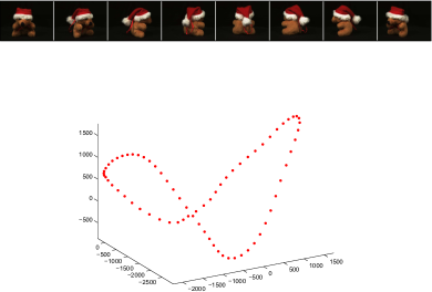
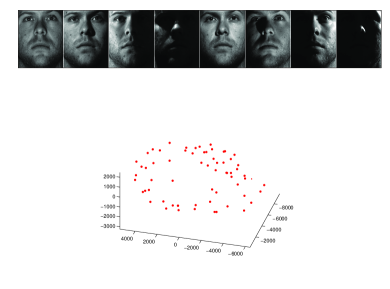
(a) Object–pose	(b) Face–illumination

Figure 1: To facilitate learning and be of discriminative use, the representation of patterns must possess a certain structure. Often, this structure is exhibited by confining the locus of members of each class to a manifold. While their higher order statistics can greatly vary (both in the original space, as well as the corresponding class manifold) depending on the manner in which data are acquired, the manifold structure can be regarded as containing only class-specific information.

The other major issue is that of devising a suitable inter-manifold metric (or rather pseudo-metric). Of particular interest to us are approaches employing canonical correlation analysis (CCA), a statistical technique that has been applied with much success to a wide variety of problems, including 3D reconstruction [21], infrared to visual image conversion [22], recognition of texture [23], objects [17, 18] and speech [24]. Broadly speaking, the key idea behind CCA is that a meaningful measure of similarity between two linear (or linearized, as touched upon previously) manifolds can be derived from the most correlated modes of variation between them. Empirical evidence suggests that this indeed is the case in a broad spectrum of problems. What makes CCA additionally attractive in practice is that canonical correlations between linear subspaces can be computed efficiently and in a numerically stable manner [25]. In this paper we propose a framework which inherits these appealing properties of CCA, whilst at the same time differing from CCA in that when applied to set matching it does not have any parameters which need to be manually tuned and is readily extended to a discriminative framework. Our approach to computing a distance between two sets can be considered manifold-based, but implicitly so, as the distance is computed without explicit manifold fitting. Rather, the distance is robustly inferred by employing second order statistics to account for the confidence that a particular observed intra-set variation corresponds to a phenomenon of interest and not noise. The proposed discriminative framework which follows the main method is based on a similar idea.

These issues and technical details pertaining to CCA and its application to set matching are addressed next, in Section 2, followed by Sections 3 and 4 introducing respectively extended CCA and discriminative extended CCA, empirical evaluation in Section 5 and a conclusion with a summary of contributions in Section 5.3.

2 Set Matching using Canonical Correlation Analysis

Consider two finite sets of vectors, $\mathcal{X}\subset\mathds{R}^{D}$ and $\mathcal{Y}\subset\mathds{R}^{D}$:

$$\mathcal{X}=\left\{\mathbf{x}_{1},\ldots,\mathbf{x}_{N}\right\}$$ (1)

$$\mathcal{Y}=\left\{\mathbf{y}_{1},\ldots,\mathbf{y}_{M}\right\}.$$ (2)

Canonical correlation analysis seeks to find a pair of latent variables or canonical vectors [26], $\mathbf{u}_{1}$ and $\mathbf{v}_{1}$, such that:

$$\exists\mathbf{a}_{1}\in\mathds{R}^{N}:~{}\mathbf{u}_{1}=\big{[}~{}\mathbf{x}_{1}~{}|~{}\ldots~{}|~{}\mathbf{x}_{N}~{}\big{]}~{}\mathbf{a}_{1}=\mathbf{X}\mathbf{a}_{1}$$ (3)

$$\exists\mathbf{b}_{1}\in\mathds{R}^{M}:~{}\mathbf{v}_{1}=\big{[}~{}\mathbf{y}_{1}~{}|~{}\ldots~{}|~{}\mathbf{y}_{M}~{}\big{]}~{}\mathbf{b}_{1}=\mathbf{Y}\mathbf{b}_{1},$$ (4)

which maximizes the canonical correlation coefficient $\rho_{1}\in[0,1]$ defined as

$$\rho_{1}=\max_{\mathbf{u}_{1},\mathbf{v}_{1}}~{}\frac{\big{\langle}\mathbf{u}_{1},\mathbf{v}_{1}\big{\rangle}}{\|\mathbf{u}_{1}\|~{}\|\mathbf{v}_{1}\|}=\max_{\mathbf{u}_{1},\mathbf{v}_{1}}~{}\frac{\mathbf{u}_{1}^{T}\mathbf{v}_{1}}{\|\mathbf{u}_{1}\|~{}\|\mathbf{v}_{1}\|}.$$ (5)

Canonical vectors and correlation coefficients of higher orders, up to $\min(N,M)$, can be defined recursively under the constraint of mutual orthogonality between all $\mathbf{u}_{i}$, as well as all $\mathbf{v}_{i}$:

$$\forall i,j.~{}i\neq j:~{}\big{\langle}\mathbf{u}_{i},\mathbf{u}_{j}\big{\rangle}=0\text{\hskip 10.0pt and \hskip 10.0pt}\big{\langle}\mathbf{v}_{i},\mathbf{v}_{j}\big{\rangle}=0$$ (6)

By construction, it holds that:

$$1\geq\rho_{1}\geq\rho_{2}\geq\ldots\rho_{min(N,M)}\geq 0$$ (7)

2.1 Set Matching Using CCA

In most cases the application of CCA to set matching considers sets of vectors over the same type of features [27, 28, 29]. For example, each vector may be a rasterized representation of an image as in Section 5 and [15, 29] for example. The usual manner of applying CCA to set matching consists of three steps. (i) First, an orthonormal basis set $\mathbf{B}_{X}$ of the subspace characterizing variations within a set is estimated using principal component analysis. Specifically, then $\mathbf{B}_{X}\in\mathbb{R}^{D\times d_{X}}$, a matrix with columns consisting of orthonormal basis vectors spanning the $d_{X}$-dimensional linear subspace embedded in a $D$-dimensional image space, can be computed from the corresponding non-centred covariance matrix $\mathbf{C}_{X}$:

$$\mathbf{C}_{X} =\frac{1}{N}~{}\sum_{i=1}^{N}\mathbf{x}_{i}~{}{\mathbf{x}_{i}}^{T},$$ (8)

as the row and column space basis of the best rank-$D$ approximation to $\mathbf{C}_{X}$:

$$\mathbf{B}_{X}=\arg\min_{\scriptsize\begin{array}[]{c}\mathbf{B}_{X}\in\mathbb{R}^{D\times d_{X}}\\ {\mathbf{B}_{X}}^{T}\mathbf{B}_{X}=I\end{array}}\min_{\scriptsize\begin{array}[]{c}~{}~{}\Lambda\in\mathbb{R}^{d_{X}\times d_{X}}\\ ~{}~{}\Lambda_{ij}=0,i\neq j\end{array}}{\big{\|}~{}\mathbf{C}_{X}-\mathbf{B}_{X}~{}\Lambda~{}{\mathbf{B}_{X}}^{T}~{}\big{\|}_{F}}^{2},$$ (13)

where $\|.\|_{F}$ is the Frobenius norm of a matrix.

The dimensionality $d_{X}$ of this subspace may be preset, it may be inferred from the distribution of data energy across eigenvector directions or indeed left equal to $N$ – the number of data points. (ii) Then, the canonical correlation coefficients $\rho_{k}$ between two subspaces $\mathbf{X}$ and $\mathbf{Y}$ can be computed using singular value decomposition (SVD) as the singular values of the matrix ${\mathbf{B}_{X}}^{T}\mathbf{B}_{Y}$ [25]. (iii) Finally, a similarity measure is computed as a function of canonical correlation coefficients. This is often done by averaging the first (i.e. the largest) few [30], although more complex learning schemes have been proposed [15].

2.1.1 Motivation and Advantages.

In intuitive terms, canonical vectors extract the most similar modes of variation between two sets, while the corresponding correlation coefficients quantify the degree to which these modes actually match. This focus on that which is common is desirable because it makes the similarity score insensitive to the presence of differing modes of variation. These may be present in the data because of different acquisition conditions, or they may indeed correspond to corrupted samples. In contrast, probability density-based methods, such as those using the Bhattacharyya distance or the Kullback-Leibler divergence, do not exhibit such robustness.

By modelling variations within a set by a subspace, canonical correlations are also inherently unaffected by uniform scaling (or, equivalently, the contrast) of individual patterns. This makes CCA-based methods particularly suitable for various computer vision tasks, where such variation may be introduced by the changes in illumination or the duration of exposure of the photosensitive medium. Learning is effectively performed on a hypersphere, as illustrated in Figure 2.

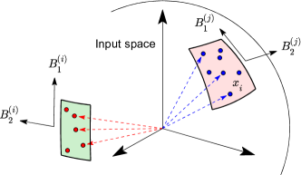
Figure 2: Canonical correlations are invariant to isotropic scale changes, such as those caused by illumination or exposure differences. This effectively constrains the learning of appearance variation to a hypersphere centred at the origin.

Finally, in many cases data variations within a single set are low dimensional making CCA-based matching practically appealing due to computational efficiency and low storage requirements.

2.1.2 Limitations of CCA.

In modelling class variation, the application of canonical correlation analysis inherently requires the partitioning of the input space into two disjoint subspaces: the class subspace $\mathbf{B}$ of observed variability, and its complementary subspace $\text{null}(\mathbf{B}^{T})$. This hard division causes several undesirable consequences.

Optimal Parameter Choice and Performance Sensitivity.

In practice the presence of noise in data is unavoidable and the optimal choice of the dimensionality of the class subspace can seldom be guaranteed [31]. Most commonly, this parameter is determined empirically, using a training and a validation set [15]. Not only through ineffective use of data, this approach is also unattractive due to its amplification of noise in the non-dominant directions of the class subspace and the loss of information in the discarded orthogonal directions.

Second Order Statistics.

To make matters worse, any principal direction is either included at an equal footing with all others in the class subspace, or entirely discarded. As we shall demonstrate, the performance of CCA-based matching is very sensitive to the choice of this parameter. This is particularly pronounced in cases suffering from limited sample size, when the number of data points needed for robust estimation for as few as two canonical correlations, is 40 to 70 times the dimensionality of the class subspace [32].

Discriminative Learning.

The described CCA-based set distance is not discriminative in nature – sets are compared in an independent, pair-wise manner, without regard for inter-class and intra-class variability. That this cannot be optimal can be seen easily by noting that depending on the application, the same two sets can be regarded as belonging to either the same or different classes: two sets of face appearance images of two different individuals correspond to the same class if the problem is that of face detection (classification to “face” and “non-face”), and different classes if it is face recognition (classification by the identity).

The first discriminative extension of CCA was proposed by Oja [33]. It consists of a linear projection of data onto a subspace which orthogonalizes basis vectors of different classes. The main shortcoming of this approach lies in its lack of robustness, with the orthogonal discriminative criterion leading to overfitting. A different linear subspace approach, which we will refer to as constrained canonical correlation analysis (C-CCA) was described by Fukui et al. [34]. They introduce a discriminative, constraint subspace, defined by the principal components corresponding to the smallest eigenvalues of the mean projection matrix across all classes:

$$\bar{\mathbf{P}}=\sum_{i}\mathbf{P}_{i}=\sum_{i}\big{(}\mathbf{B}_{i}~{}{\mathbf{B}_{i}}^{T}\big{)}$$ (14)

The computation of canonical correlations is then preceded by a linear projection to the constraint subspace, as illustrated conceptually in Figure 3. For the optimal size of its dimensionality, C-CCA generally outperforms Oja’s orthogonal subspace method [35], as well as non-discriminative CCA [36, 37]. However, ensuring that the optimal value is chosen is difficult. In addition, the construction of the described constraint subspace is ad hoc in nature – it does not maximize any meaningful discriminative function and it does not take into account inter-class variation, relying purely on intra-class variability. A solution to this problem was proposed by Kim et al. [35], in the form of an iterative method which incrementally adjusts the optimal projection subspace to maximize expected inter-class to intra-class canonical correlations. This is achieved at a great computational cost, the loss of closed-form computability and with the restriction of discrimination between only two classes. Also, just like the previous two approaches, this method suffers from an increased number of free parameters and the “all or nothing” modelling of class distributions.

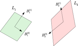
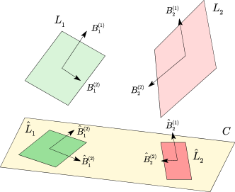
(a) CCA	(b) C-CCA

Figure 3: A conceptual illustration of the principles underlying set matching using a similarity measure based on (a) canonical correlation analysis (CCA) and (b) its discriminative extension, constrained canonical correlation analysis (C-CCA). Both methods effectively compute the angles between subspaces corresponding to vector sets, preceded by a quasi-discriminative projection in the case of C-CCA.

Nonlinearity.

Finally, for completeness, we briefly mention that simple CCA assumes linear intra-class variability. Effective solutions to this problem have been described in the literature, involving either piece-wise linearization of class manifolds [15] or their “unfolding” [38, 13]. All of these approaches eventually reduce to the computation of CCA in its original form and can thus without modification be applied with the methods we propose in this paper.

3 Extended Canonical Component Analysis (E-CCA)

Motivated by the standard canonical component analysis, in this section we too seek to find the most correlated modes of variation within two sets. However, unlike before, we wish to do so without discarding any data i.e. without the partitioning of the input space into principal (relevant) and complementary (noise) subspaces. As explained in Section 2.1.2 this partitioning is a source of major problems when CCA is applied to set matching. For illustration, consider the problem of matching sets of images (see Section 5 for a practical example). Generally, each of the image pixels is affected by noise which contains a non-correlated component across different pixels. This means that if sufficient data is available, each of the image sets will exhibit variation in all directions of the input image space. Consequently, all of the canonical correlations between any two sets would be $1.0$ if subspace projection described in Section 2.1 was not applied (i.e. if the input space was not partitioned). To avoid the need for this projection and the potential for information loss thus effected, we wish to derive a CCA inspired set similarity measure which takes into account the confidence that the observed mode of variation is indeed due to data variability and not noise. We achieve this by incorporating second order statistics into the similarity measure.

Our approach is motivated by observing that for the pair of canonical vectors $\mathbf{u}_{1}$ and $\mathbf{v}_{1}$ in Equations (3)-(4) there exists a direction $\mathbf{w}_{1}$ for which:

$$\mathbf{u}_{1}={\mathbf{B}_{X}}{\mathbf{B}_{X}}^{T}\mathbf{w}_{1}$$ (15)

$$\mathbf{v}_{1}={\mathbf{B}_{Y}}{\mathbf{B}_{Y}}^{T}\mathbf{w}_{1}$$ (16)

The first multiplication, by ${\mathbf{B}_{X}}^{T}$ or ${\mathbf{B}_{Y}}^{T}$, has the effect of removing any variation not spanned by the columns of $\mathbf{B}_{X}$ and $\mathbf{B}_{Y}$ respectively (the two principal subspaces), while the second multiplication by $\mathbf{B}_{X}$ or $\mathbf{B}_{Y}$, re-embeds the vectors in the original input space.

The first canonical correlation coefficient can then be written as:

$$\rho_{1} =\frac{{\mathbf{w}_{1}}^{T}~{}{\mathbf{B}_{X}}{\mathbf{B}_{X}}^{T}\mathbf{B}_{Y}{\mathbf{B}_{Y}}^{T}~{}\mathbf{w}_{1}}{\|{\mathbf{B}_{X}}^{T}\mathbf{w}_{1}\|~{}\|{\mathbf{B}_{Y}}^{T}\mathbf{w}_{1}\|}$$ (17)

$$=\frac{{\mathbf{w}_{1}}^{T}~{}{\mathcal{W}(\hat{\mathbf{\Sigma}}_{X})}^{T}~{}\mathcal{W}(\hat{\mathbf{\Sigma}}_{Y})~{}\mathbf{w}_{1}}{\|{\mathbf{B}_{X}}^{T}\mathbf{w}_{1}\|~{}\|{\mathbf{B}_{Y}}^{T}\mathbf{w}_{1}\|}$$ (18)

where $\mathcal{W}(\ldots)$ is the covariance matrix whitening function [39], and:

$$\hat{\mathbf{\Sigma}}_{X}=\mathbf{B}_{X}\hat{\mathbf{\Lambda}}_{X}{\mathbf{B}_{X}}^{T}$$ (19)

$$\hat{\mathbf{\Sigma}}_{Y}=\mathbf{B}_{Y}\hat{\mathbf{\Lambda}}_{Y}{\mathbf{B}_{Y}}^{T}$$ (20)

Instead of a normalized projection of the vector $\mathbf{w}_{1}$ onto a subspace, say $\mathbf{B}_{X}$, consider its transformation effected by the corresponding “deviation” matrix $\mathbf{\Upsilon}_{X}$ (also positive semi-definite and symmetric) which we define as:

$$\mathbf{\Upsilon}_{X} =\left(\mathbf{\Sigma}_{X}\right)^{1/2}={\small\mathbf{V}_{X}~{}\begin{bmatrix}\sqrt{\lambda_{X}^{(1)}}&0&0&0\\ 0&\sqrt{\lambda_{X}^{(2)}}&0&0\\ 0&0&\ddots&0\\ 0&0&0&\sqrt{\lambda_{X}^{(D)}}\\ \end{bmatrix}}~{}{\mathbf{V}_{X}}^{T}$$

$$=\mathbf{V}_{X}~{}\left(\mathbf{\Lambda}_{X}\right)^{1/2}~{}{\mathbf{V}_{X}}^{T}$$ (21)

where:

$$\mathbf{\Sigma}_{X}=\mathbf{X}\mathbf{X}^{T}=\mathbf{V}_{X}~{}\mathbf{\Lambda}_{X}~{}{\mathbf{V}_{X}}^{T}$$ (22)

is the full data covariance matrix. The said transformation anisotropically scales its input, amplifying it in the directions in which $\mathcal{X}$ exhibits significant variability (large $\lambda_{X}^{(i)}$) and attenuating in those with little (or indeed no) variability (small $\lambda_{X}^{(i)}$), as illustrated in Figure 4. This effect can be considered a generalization of the projection described in Equation (20) – while in the application of standard CCA all variation in the complementary subspace is discarded and the variation in the principal subspace whitened, here the transformation has the effect of smoothly emphasizing or de-emphasizing different directions of variability according to its extent (specifically, proportionally to the standard deviation in the corresponding direction). In the special case of data which exhibits isotropic variability constrained to a subspace the result is exactly the same as in Equation (20) (up to scale).

Motivated by this intuition and extending the analogy to Equation (18), we seek such unit vector $\hat{\mathbf{w}}_{1}$ whose projections by $\mathbf{\Upsilon}_{X}$ and $\mathbf{\Upsilon}_{Y}$ have the highest degree of correlation. Formally, we define the first extended canonical correlation coefficient $\psi_{1}$ between $\mathcal{X}$ and $\mathcal{Y}$ as:

$$\psi_{1} =\max_{\hat{\mathbf{w}}_{1}}~{}\big{\{}(\mathbf{\Upsilon}_{X}~{}\hat{\mathbf{w}}_{1})^{T}~{}(\mathbf{\Upsilon}_{Y}~{}\hat{\mathbf{w}}_{1})\big{\}}$$ (23)

$$=\max_{\hat{\mathbf{w}}_{1}}~{}\big{\{}{\hat{\mathbf{w}}_{1}}^{T}~{}{\mathbf{\Upsilon}_{X}}^{T}~{}\mathbf{\Upsilon}_{Y}~{}\hat{\mathbf{w}}_{1}\big{\}}$$ (24)

$$=\max_{\hat{\mathbf{w}}_{1}}~{}\big{\{}{\hat{\mathbf{w}}_{1}}^{T}~{}{\mathbf{\Upsilon}_{X}}^{T}~{}\mathbf{\Upsilon}_{Y}~{}\hat{\mathbf{w}}_{1}\big{\}}$$ (25)

$$=\max_{\hat{\mathbf{w}}_{1}}~{}\big{\{}{\hat{\mathbf{w}}_{1}}^{T}~{}\mathbf{\Phi}_{XY}~{}\hat{\mathbf{w}}_{1}\big{\}},$$ (26)

under the constraint:

$$\|\hat{\mathbf{w}}_{1}\|=1.$$ (27)

The key idea here is that this measure will favour those directions of the space in which both $\mathcal{X}$ and $\mathcal{Y}$ have significant variability (it is “amplified” both by $\mathbf{\Upsilon}_{X}$ and $\mathbf{\Upsilon}_{Y}$). Similarly, a direction in which $\mathbf{\Upsilon}_{X}$ (say) exhibits significant variability, but $\mathbf{\Upsilon}_{Y}$ does not, will contribute to $\hat{\mathbf{w}}_{1}$ less, while a direction in which neither of the sets exhibit significant variability will be greatly de-emphasized and have little effect on $\hat{\mathbf{w}}_{1}$.

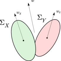
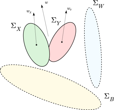
(a) E-CCA	(b) DE-CCA

Figure 4: A conceptual illustration of the principles underlying set matching using a similarity measure based on the proposed (a) extended canonical correlation analysis (E-CCA) and (b) its discriminative variant, discriminative extended canonical correlation analysis (DE-CCA). Set similarity is computed by considering projective space distortions corresponding to the sets’ covariances and, in the case of DC-CCA, discriminative inter-class and intra-class covariances inferred from training data.

Note that although matrices $\mathbf{\Upsilon}_{X}$ and $\mathbf{\Upsilon}_{Y}$ are symmetric, their product is not. Nonetheless, $\mathbf{\Phi}_{XY}$ is positive semi-definite. This is because linear transformations effected by $\mathbf{\Upsilon}_{X}$ and $\mathbf{\Upsilon}_{Y}$ involve no rotation, reflection or shearing, i.e. they can be expressed purely as a combination of orthogonal projection, and (generally anisotropic) scaling. Thus $\psi_{1}$ is maximized when $\hat{\mathbf{w}}$ is in the direction of the eigenvector of $\mathbf{\Phi}_{XY}$ corresponding to its largest eigenvalue, for which:

$$\psi_{1}=\lambda_{\Phi}^{(1)},$$ (28)

where $\lambda_{\Phi}^{(1)}\geq\lambda_{\Phi}^{(2)}\geq\ldots\lambda_{\Phi}^{(D)}\geq 0$ are the eigenvalues of $\mathbf{\Phi}_{XY}$.

When classical canonical correlation analysis is applied to pattern recognition in practice, only the first few correlation coefficients are computed. This is largely a consequence of the trade-off between the accuracy of matching and its speed. Our approach does not suffer from the same weakness. Extending the analysis to higher order extended correlation coefficients, we can quantify the degree of agreement between variations observed in sets $\mathcal{X}$ and $\mathcal{Y}$ as:

$$\mu_{XY}=\frac{\sum_{i=1}^{D}\psi_{i}}{\sum_{i=1}^{D}\sqrt{\lambda_{X}^{(i)}\lambda_{Y}^{(i)}}}$$ (29)

More elaborate combinations of $\psi_{i}$ are possible, e.g. as described in [15], but here we adopt a simple normalized summation because it lends itself to particularly efficient computation, as we will show shortly.

Note that $\mu_{XY}$ reaches its maximum maximorum when $\mathbf{\Upsilon}_{X}$ and $\mathbf{\Upsilon}_{Y}$ share the same eigenspace and when their eigenvectors of the same rank (with respect to the magnitude of the corresponding eigenvalue) are aligned. However, in general:

$$0\leq\mu_{XY}\leq 1.$$ (30)

The class similarity $\mu_{XY}$ in Equation (29) can be rapidly computed by noticing that:

$$\sum_{i=1}^{D}\psi_{i}=\text{Tr}~{}\big{[}~{}\mathbf{\Phi}_{XY}~{}\big{]},$$ (31)

while the values of $\lambda_{X}^{(1)},\ldots,\lambda_{X}^{(D)}$ and $\lambda_{Y}^{(1)},\ldots,\lambda_{Y}^{(D)}$ are estimated in the same manner as in the case of classical CCA.

It is important to observe that in Equation (26) there is no concern of an ill-defined result because of a vanishing denominator (unlike in the case of the method described in [40] for example). Specifically, since $\lambda^{(i)}_{X}$ and $\lambda^{(i)}_{Y}$ are ordered in magnitude, the product $\lambda^{(1)}_{X}~{}\lambda^{(1)}_{Y}$ cannot be 0 as both sets $\mathcal{X}$ and $\mathcal{Y}$ are assumed to contain at least some variability. Indeed, this is a necessary condition both for classical CCA and the proposed method to be meaningful in this context.

4 Discriminative Extended Canonical Component Analysis (DE-CCA)

In the previous section we derived a principled extension of canonical correlation analysis suitable for matching sets of patterns constrained to linear subspaces. We addressed the inherent limitations of CCA when applied on this problem: the inevitable “hard” partitioning of the input space, as well the practical difficulty of parameter estimation. Unlike classical CCA, we now show that our method readily lends itself to a discriminative learning framework.

In Section 3 we considered space transformation by means of projection using the square root of the class covariance matrix:

$$\mathbf{w}_{1}\longrightarrow\mathbf{\Upsilon}_{X}\mathbf{w}_{1}=\left(\mathbf{\Sigma}_{X}\right)^{1/2}\mathbf{w}_{1}.$$ (32)

Its effect is the amplification of modes of variation common to the input vector $\mathbf{w}_{1}$ and the set $\mathcal{X}$. However, this is achieved without any knowledge of variability both between and within different classes. Here we capture these through two covariance matrices, the normalized inter-class scatter matrix $\mathbf{\Sigma}_{B}$ and the mean intra-class scatter matrix $\mathbf{\Sigma}_{W}$. Using the notation $\mathbf{Z}_{i}$ for different training set data matrices $i=1,\ldots,N_{C}$ (each corresponding to a different class) and denoting their members by $\left\{\mathbf{z}_{i1},\mathbf{z}_{i2},\ldots\right\}$, we define the normalized inter-class scatter matrix as follows:

$$\mathbf{\Sigma}_{B}=\frac{1}{N_{C}}~{}\sum_{i=1}^{N_{C}}\left(\frac{E[\mathbf{Z}_{i}]}{\|E[\mathbf{Z}_{i}]\|}-\mathbf{m}\right)$$ (33)

where:

$$\mathbf{m}=\frac{1}{N_{C}}~{}\sum_{i=1}^{N_{C}}\frac{E[\mathbf{Z}_{i}]}{\|E[\mathbf{Z}_{i}]\|}.$$ (34)

Note that the explicit normalization of class data means $E[\mathbf{Z}_{i}]$ in Equation (33) is necessary here (see Section 2.1.1). The mean intra-class scatter matrix is simply:

$$\mathbf{\Sigma}_{W}=\frac{1}{N_{C}}~{}\sum_{i=1}^{N_{C}}{\mathbf{Z}_{i}}^{T}\mathbf{Z}_{i}=\frac{1}{N_{C}}~{}\sum_{i=1}^{N_{C}}{\mathbf{\Sigma}_{Z_{i}}}$$ (35)

Our definitions of inter-class and intra-class matrices are similar to those used in Fisher’s discriminant analysis [39].

The two scatter matrices are then used to further transform an input vector, first by accentuating its components in the direction of common intra-class variations and then by attenuating those corresponding to inter-class variability:

$$\mathbf{w}_{1}\longrightarrow\left({\mathbf{\Sigma}_{B}}\right)^{-1/2}\left({\mathbf{\Sigma}_{W}}\right)^{1/2}\mathbf{\Upsilon}_{X}\mathbf{w}_{1}.$$ (36)

The intuition behind this transformation is exactly the same as that for the non-discriminative version in Section 3. Instead of partitioning the space into discriminative and non-discriminative subspaces and projecting the data onto the former, like in CCA for example, our transformation of data is smoother in nature. While a projection onto the discriminative subspace entirely aligns the data with the subspace, our transformation instead realigns the data smoothly first by emphasizing discriminative directions (according to the inter-class scatter matrix) and then by further de-emphasizing the non-discriminative ones (according to the intra-class scatter matrix). The idea is illustrated conceptually in Figure 4(b). Note that the aforementioned directions are not explicitly determined. Rather, inter- and intra-class variances are automatically combined into the optimal weighting matrix $\left({\mathbf{\Sigma}_{B}}^{-1}{\mathbf{\Sigma}_{W}}\right)^{1/2}$. Formulating a criterion similar to that in Equation (26) now leads to eigenvalue decomposition of the matrix $\hat{\mathbf{\Phi}}_{XY}$:

$$\hat{\mathbf{\Phi}}_{XY}=\mathbf{\Upsilon}_{X}\mathbf{P}\mathbf{\Upsilon}_{Y}$$ (37)

where:

$$\mathbf{P}=\left({\mathbf{\Sigma}_{W}}\right)^{1/2}\left({\mathbf{\Sigma}_{B}}\right)^{-1}\left({\mathbf{\Sigma}_{W}}\right)^{1/2}$$ (38)

Just as $\mathbf{\Phi}_{XY}$ in the non-discriminative case and using the same argument as on page 4, $\hat{\mathbf{\Phi}}_{XY}$ can be recognized as a non-symmetric but nonetheless positive semi-definite matrix. Thus, the first discriminative extended canonical correlation coefficient is equal to its largest eigenvalue and, as in Equation (29), the overall similarity of sets $\mathcal{X}$ and $\mathcal{Y}$ becomes:

$$\hat{\mu}_{XY} =\frac{\sum_{i=1}^{D}\lambda_{\phi}^{(i)}}{\sum_{i=1}^{D}\sqrt{\lambda_{X}^{(i)}\lambda_{Y}^{(i)}}}=\frac{\text{Tr}~{}\left[\hat{\mathbf{\Phi}}_{XY}\right]}{\sum_{i=1}^{D}\sqrt{\lambda_{X}^{(i)}~{}\lambda_{Y}^{(i)}}}$$ (39)

5 Experimental Evaluation

We empirically examined the validity of theoretical arguments put forward in the preceding sections on the problem of matching sets of images of faces. To make our experiments as directly comparable as possible to those in the published previous work most closely related to ours, we evaluated the proposed methods on a database already widely used for this purpose (e.g. see [40, 15]) and described in detail in [41].

This database contains video sequences of face motion for 100 individuals of varying ages and ethnicities. For each person in the database there are 7 sequences of the person performing loosely constrained, pseudo-random motion (significant translation, yaw and pitch, negligible roll) for 10 s, as shown on an example in Figure 5(a). Each sequence was acquired in a different illumination setting as illustrated in Figure 5(b). Sequences were acquired at 10 fps and in $320\times 240$ pixel resolution (face size $\approx 60$ pixels). The users were asked to approach the camera while performing arbitrary head motion. Although the illumination was kept constant throughout each sequence, there is some variation in the manner in which faces were lit due to the change in the relative position of the user with respect to the lighting sources, as shown in Figure 5(c).

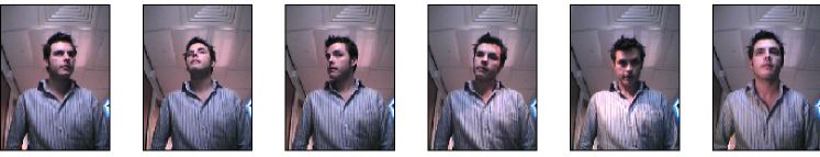
(a) Raw video frames

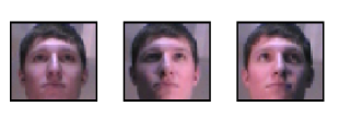
(b) Different illuminations

(c) Same illumination for different individuals

Figure 5: (a) Frames from typical video sequences in the database used for evaluation. (b) Different illumination conditions used to acquire data, illustrated on manually selected frontal faces. (c) Five different individuals in the illumination setting number 6. In spite of the same spatial arrangement of light sources, their effect on the appearance of faces changes significantly due to variations in people’s heights, the ad lib chosen position relative to the camera etc.

Faces were detected automatically using the cascaded detector of Viola and Jones [42] are rescaled to the uniform resolution of $50\times 50$ pixels which is approximately the average size of a detected face (see [43] for a related discussion). Face image patches were then converted into vectors by column-wise rasterization, each video sequence thus producing a set of vectors in the $\mathds{R}^{2500}$ space. Different distance measures between sets were evaluated in the context of one-to-many matching. In other words, image sets extracted from video sequences of different individuals in a particular setting were used as training data while querying was performed using sets corresponding to a different illumination. Each query set was associated with the best matching training set. In this manner, we investigated:

• the sensitivity of the classical CCA to the number of correlation coefficients,
  

• the sensitivity of the C-CCA to the dimensionality of the constraining subspace,
  

• the performance of the proposed E-CCA distance measure, and
  

• the performance of the proposed DE-CCA distance measure.

5.1 Results and Discussion

A summary of the key results is shown in Table 1. As expected in the case of data with such complex variability as exhibited by face appearance images, the performance of the classical CCA-based matching is greatly affected by the number of canonical correlation coefficients used to compute the set-to-set similarity measure. When their number is increased from one to two, the average performance is improved by 59%, and further by 78% for three coefficients. Additional sensitivity of the method to free parameter selection can be observed in Figure 6(a), which illustrates the importance of the dimensionality of class subspaces.

It is revealing to notice that while an increase in the number of computed canonical correlations improves the average rate of correct identification, the confidence in the recognition decision (quantified by the deviation of the correct identification rate across different test and query illumination conditions) actually worsens. This phenomenon can be explained by observing that increasing the number of coefficients does not improve matching decisions in the most challenging cases (corresponding to test and query illumination combinations that result in the lowest correct identification rates). In other words, in these cases, the variations present in different appearance sets corresponding to the same person are indeed very unlike one another, and the only way of producing an improvement is by incorporating discriminative constraints.

Table 1: A summary of experimental results. Shown are the average correct recognition rate across different illuminations used for training and querying, and its standard deviation. Even for the optimal choice of parameters, which is impossible to ensure in practice, classical canonical correlation analysis (CCA: a non-discriminative approach) and its constrained extension (C-CCA: discriminative) were outperformed by the proposed methods which are parameter-free.

Method	CCA			C-CCA (3 cc)
Parameters	1 cc	2 cc	3 cc	-15d	-25d	-50d	-100d
Mean correct recognition rate	42.2	67.0	75.1	78.7	83.6	83.2	74.4
Recognition rate deviation	10.6	13.9	13.5	11.1	8.3	9.0	15.4

Method	E-CCA	DE-CCA
Mean correct recognition rate	83.4	88.8
Recognition rate deviation	9.6	7.8

The results obtained using constrained CCA highlight further limitations of classical canonical correlation analysis in set matching. In addition to the sensitivity of the method to the free parameters shared with CCA – the number of canonical correlations used to compute set similarities and the dimensionality of class subspaces, illustrated for C-CCA in Figure 6(b) – an additional free parameter is introduced in the form of the dimensionality of the constraint subspace. Discriminative projection of data was found to improve performance only for constraint subspace dimensionalities greater than $(D-95)$, which is a narrow range of just $\sim$3.8% of the input space dimensionality $D=2500$. In this range, the mean recognition rate is increased and its deviation decreased. Peak correct recognition rate of 83.6% (33% reduction in error rate compared to simple CCA) is achieved when three canonical correlation coefficients are used and the dimensionality of the constraint subspace set equal to $(D-25)$. However, a suboptimal choice of the constraint subspace dimensionality can rapidly lead to significant worsening of performance, as shown in Figure 6(c). This is a major limitation of C-CCA, as there is no fundamental theoretical basis which could facilitate the inference of this parameter.

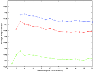
(a) Canonical correlation analysis

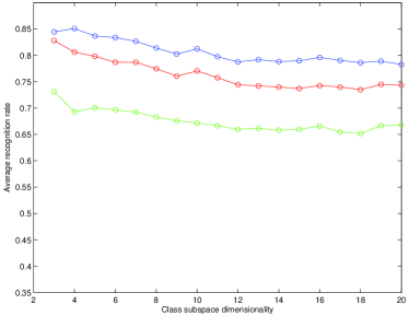
(b) Extended canonical correlation analysis

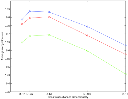
(c) Discriminative extended canonical correlation analysis

Figure 6: The measured variation of the correct recognition rate averaged over different illumination conditions used for training and querying, as a function of the dimensionality of the constraint subspace and the number of canonical correlation coefficients used for matching (green=1, red=2, blue=3). Optimal performance is achieved using three canonical correlations and $(D-25)$-dimensional constraint subspace.

As this paper argued in detail, the problem of free parameter choice is made entirely obsolete by our use of second order statistics. The proposed E-CCA was found to significantly outperform not only CCA but C-CCA as well, and remarkably for all values of their free parameters, as can be seen in Table 1. Practically, this is a major advantage of our approach, due to the difficulty of ensuring optimal parameter selection for C-CCA. Theoretically, this confirms the premise set forth in Section 1 which emphasizes the loss of discriminative information in discarding higher order statistics of class variability. This is an important result given that unlike E-CCA, C-CCA is a discriminative approach. With that in mind, it is not surprising that our discriminative method, DE-CCA, improves performance even further, decreasing the error rate by 32% from C-CCA – see Table 1.

5.2 Qualitative Insight

It is insightful to visually examine the modes of the most probable common variability between sets of the same and different classes, extracted by the proposed methods. These can be found as the dominant eigenvectors of the matrix $\mathbf{\Phi}_{XY}$ in the case of E-CCA (see Section 3), and $\hat{\mathbf{\Phi}}_{XY}$ (see Section 4) in the case of DE-CCA. Examples, visualized as images, are shown in Figure 7. Notice that E-CCA manages to find meaningful common modes even when the two sets correspond to different people, just as it does when they show the same person – it effectively matches similar appearing illumination effects. This is a consequence of geometric and textural similarity of human faces, which makes face recognition so difficult. By learning a discriminative criterion, matching using DE-CCA has the consequence of de-emphasizing confounding inter-personal variability and amplifying intra-personal information.

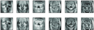
(a) E-CCA, same class

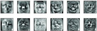
(b) E-CCA, different classes

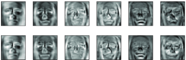
(c) DE-CCA, same class

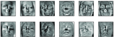
(d) DE-CCA, different classes

Figure 7: The most similar 6 modes of variation extracted using (a,b) E-CCA and (c,d) DE-CCA using sets corresponding to the same person in different illuminations (a,c) and different persons. In the case of same class matching, both methods successfully extract common directions of appearance change between two sets. The benefit of DE-CCA is more pronounced when sets of images of different persons are matched – E-CCA erroneously manages to find rather more alike modes of variation by effectively matching on common illumination, while the discriminative algorithm correctly learns and de-emphasizes such confounding factors.

5.3 Summary and Conclusions

In this paper we proposed a novel framework for matching vector sets. Our approach is based on inference of the most similar modes of variability within two sets. This led to a comparison with increasingly popular canonical correlation analysis-based methods. These were discussed in detail and it was shown, both theoretically and empirically, that they have significant practical limitations of which the most important are: (i) the presence of free parameters which cannot be inferred from the data, (ii) non-robust partitioning of the space into class and non-class subspaces, and (iii) intractability of discriminative learning. In contrast, the proposed extended canonical correlation analysis-based method inherently accounts for uncertainty in data, inferring the most likely common modes of variability. What is more, it is shown that this can be achieved without the loss of attractive computational efficiency of canonical correlation analysis, whereby set similarity is effectively reduced to the computation of the trace of a matrix. The proposed framework was then extended into a discriminative learning scheme which, unlike in the case of classical canonical correlation analysis, follows naturally. Finally, our theoretical arguments were empirically verified on the task of set-based face recognition. The proposed methods were shown superior even for the optimal choice of parameters of the classical canonical correlation analysis-based methods, which is impossible to ensure in practice.

References

- [1] S. Satoh. Comparative evaluation of face sequence matching for content-based video access. In Proc. IEEE International Conference on Automatic Face and Gesture Recognition (FG), pages 163–168, 2000.
- [2] E. P. Vivek and N. Sudha. Robust hausdorff distance measure for face recognition. Pattern Recognition (PR), 40(2):431–442, 2007.
- [3] W. Fan and D-Y. Yeung. Face recognition with image sets using hierarchically extracted exemplars from appearance manifolds. In Proc. IEEE International Conference on Automatic Face and Gesture Recognition (FG), pages 177–182, 2006.
- [4] G. Shakhnarovich, J. W. Fisher, and T. Darrel. Face recognition from long-term observations. In Proc. European Conference on Computer Vision (ECCV), 3:851–868, 2002.
- [5] A. Bhattacharyya. On a measure of divergence between two statistical populations defined by their probability distributions. Bulletin of the Calcutta Mathematical Society, 35:99– 109, 1943.
- [6] H. Chernoff. A measure of asymptotic efficiency of tests for a hypothesis based on a sum of observation. Annals of Mathametical Statistics, 23:493–507, 1952.
- [7] S. Sinanović and D. H. Johnson. Toward a theory of information processing. Signal Processing, 87:1326–1344, 2007.
- [8] O. Arandjelović and R. Cipolla. An information-theoretic approach to face recognition from face motion manifolds. Image and Vision Computing (special issue on Face Processing in Video), 24(6):639–647, 2006.
- [9] R.A. Kullback, S. Leibler. On information and sufficiency. Annals of Mathematical Statistics, 22(1):79 –86, 1951.
- [10] O. Arandjelović and R. Cipolla. Achieving robust face recognition from video by combining a weak photometric model and a learnt generic face invariant. Pattern Recognition (PR), 46(1):9–23, 2013.
- [11] K. Lee, J. Ho, and D. Kriegman. Nine points of light: Acquiring subspaces for face recognition under variable lighting. In Proc. IEEE Conference on Computer Vision and Pattern Recognition (CVPR), 1:519–526, 2003.
- [12] I. Borg and P. Groenen. Modern Multidimensional Scaling: theory and applications. Springer-Verlag, New York, 2nd edition, 2005.
- [13] S. Roweis and L. K. Saul. Nonlinear dimensional reduction by locally linear embedding. Science, 290, 2001.
- [14] B. K. Gunturk, Y. Batur, A. U. Altunbasak, M. H. Hayes, and R. M. Mersereau. Eigenface-domain super-resolution for face recognition. IEEE Transactions on Image Processing (TIP), 12(5):597–606, 2003.
- [15] T-K. Kim, O. Arandjelović, and R. Cipolla. Boosted manifold principal angles for image set-based recognition. Pattern Recognition (PR), 40(9):2475–2484, 2007.
- [16] F. Bach and M. I. Jordan. Kernel independent component analysis. Journal of Machine Learning Research (JMLR), 3:1–48, 2002.
- [17] L. Wolf and A. Shashua. Learning over sets using kernel principal angles. Journal of Machine Learning Research (JMLR), 4(10):913–931, 2003.
- [18] T. Melzer, M. Reiter, and Bischofm H. Appearance models based on kernel canonical correlation analysis. Pattern Recognition (PR), 36(9):1961–1971, 2003.
- [19] M-H. Yang. Kernel eigenfaces vs. kernel fisherfaces: Face recognition using kernel methods. In Proc. IEEE International Conference on Automatic Face and Gesture Recognition (FG), pages 215–220, 2002.
- [20] K. Fukumizu, F. Bach, and A. Gretton. Consistency of kernel canonical correlation analysis. Journal of Machine Learning Research (JMLR), 8:361–383, 2007.
- [21] M. Reiter, R. Donner, G. Langs, and H. Bischof. 3D and infrared face reconstruction from RGB data using canonical correlation analysis. In Proc. IEEE International Conference on Pattern Recognition (ICPR), 1:425 –428, 2006.
- [22] M. Dou, C. Zhang, P. Hao, and J. Li. Converting thermal infrared face images into normal gray-level images. Lecture Notes in Computer Science (LNCS), 4844:722–732, 2007.
- [23] P. Saisan, G. Doretto, Y.N. Wu, and S. Soatto. Dynamic texture recognition. In Proc. IEEE Conference on Computer Vision and Pattern Recognition (CVPR), 2:58–63, 2001.
- [24] K. Choukri and G. Chollet. Adaptation of automatic speech recognizers to new speakers using canonical correlation analysis techniques. Computer Speech & Language, 1(2):95–107, 1986.
- [25] Å. Björck and G. H. Golub. Numerical methods for computing angles between linear subspaces. Mathematics of Computation, 27(123):579 –594, 1973.
- [26] H. Hotelling. Relations between two sets of variates. Biometrika, 28:321–372, 1936.
- [27] M. Hua and J. Peib. Clustering in applications with multiple data sources - a mutual subspace clustering approach. Neurocomputing, 92:133 –144, 2005.
- [28] K. Hotta. Local co-occurrence features in subspace obtained by kpca of local blob visual words for scene classification. Pattern Recognition (PR), 45(10):321–372, 2012.
- [29] O. Arandjelović. Colour invariants under a non-linear photometric camera model and their application to face recognition from video. Pattern Recognition (PR), 45(7):2499– 2509, 2012.
- [30] A. Maki and K. Fukui. Ship identification in sequential ISAR imagery. Machine Vision and Applications, 15(3), 2004.
- [31] Z. Gou and C. Fyfe. Generalised canonical correlation analysis. In Proc. International Conference on Intelligent Data Engineering and Automated Learning, Data Mining, Financial Engineering, and Intelligent Agents (IDEAL), pages 164–173, 2009.
- [32] R. Barcikowski and J.P. Stevens. A Monte Carlo study of the stability of canonical correlations, canonical weights, and canonical variate-variable correlations. Multivariate Behavioral Research, 10:353–364, 1975.
- [33] E. Oja. Subspace Methods of Pattern Recognition. Research Studies Press and J. Wiley, 1983.
- [34] K. Fukui and O. Yamaguchi. Face recognition using multi-viewpoint patterns for robot vision. International Symposium of Robotics Research, 2003.
- [35] T-K. Kim, J. V. Kittler, and R. Cipolla. Discriminative learning and recognition of image set classes using canonical correlations. IEEE Transactions on Pattern Analysis and Machine Intelligence (TPAMI), 29(6):1005–1018, 2007.
- [36] M. Nishiyama, O. Yamaguchi, and K. Fukui. Face recognition with the multiple constrained mutual subspace method. In Proc. Audio and Video-Based Biometric Person Authentication, pages 71–80, 2005.
- [37] O. Arandjelović and R. Cipolla. A new look at filtering techniques for illumination invariance in automatic face recognition. In Proc. IEEE International Conference on Automatic Face and Gesture Recognition (FG), pages 449–454, 2006.
- [38] K. Fukui, B. Stenger, and O. Yamaguchi. A framework for 3D object recognition using the kernel constrained mutual subspace method. In Proc. Asian Conference on Computer Vision (ACCV), pages 315–324, 2006.
- [39] R. O. Duda, P. E. Hart, and D. G. Stork. Pattern Classification. John Wily & Sons, Inc., New York, 2nd edition, 2000.
- [40] O. Arandjelović and R. Cipolla. Face set classification using maximally probable mutual modes. In Proc. IEEE International Conference on Pattern Recognition (ICPR), pages 511–514, 2006.
- [41] O. Arandjelović. Computationally efficient application of the generic shape-illumination invariant to face recognition from video. Pattern Recognition (PR), 45(1):92–103, 2012.
- [42] P. Viola and M. Jones. Robust real-time face detection. International Journal of Computer Vision (IJCV), 57(2):137–154, 2004.
- [43] O. Arandjelović. Recognition from appearance subspaces across image sets of variable scale. In Proc. British Machine Vision Conference (BMVC), 2010. DOI: 10.5244/C.24.79.