On the quantum-field description of many-particle
Bose systems with spontaneously broken symmetry

Abstract

A quantum-field approach to studying the Bose systems at finite temperatures and in states with spontaneously broken symmetry, in particular in a superfluid state, is proposed. A generalized model of a self-consistent field (SCF) for spatially inhomogeneous many-particle Bose systems is used as the initial approximation. A perturbation theory has been developed, and a diagram technique for temperature Green’s functions (GFs) has been constructed. The Dyson’s equations joining the eigenenergy and vertex functions have been deduced.

The application of quantum-field methods to the description of interacting Bose particles meets the considerable difficulties. The nature of these difficulties is associated with the fact that, at sufficiently low temperatures, the Bose systems are in the state with a with spontaneously broken phase symmetry. Therefore, one has to utilize the quantum-field methods which have to be formulated with regard for the symmetry breakdown. A success in the utilization of the quantum-field perturbation theory essentially depends on the correct choice of the zeroth approximation. As a rule, in the standard approximation, the model of non-interacting particles is used as an initial approximation, and the interaction Hamiltonian is considered as a perturbation AGD . Such a decomposition of the Hamiltonian turns out to be inefficient under the utilization of perturbation theory for the investigation of the systems with spontaneously broken symmetry. Furthermore, if a model of the ideal Bose gas with a condensate is chosen as the zero approximation, the Wick’s theorems, which are the basis of the perturbation theory and diagram technique in a field theory, are inapplicable due to the presence of the Bose condensate. However, S.T. Belyaev Belyaev managed to overcome the obstacles using the N.N. Bogolyubov’s idea Bogolyubov1 of a substitution of the operators of particles with zero momentum by c -numbers. The Belyaev’s approach was further developed in Ref. HP . However, this approach is not sufficiently general. In particular, it is not clear how the approach can be extended to spatially inhomogeneous Bose systems, in which the Bose condensate contains not only the particles with zero momentum, but also the particles with nonzero one. What is more, the substitution of an operator by a c -number, which is considered as a variational parameter, is an approximation that essentially influences the theory structure. Later on, in works NN ; PS , the attention was paid to the paradoxicality of some results obtained within the frames of the theory based on the model of ideal Bose gas. A modified variant of the quantum-field theory N developed to overcome the noted difficulties contains a lot of assumptions and cannot be considered as consistently microscopic.

The quantum-field description of the many-particle systems with broken symmetry can be made more consistent by means of the utilization of a SCF model as an initial approximation. For the case of Fermi particles, a choice of such zero approximation for a many-particle problem was proposed by Goldstone and Hubbard (see references 2 and 9 in a book of collected articles PMQT ). A description of the quantum-field methods constructed on the basis of the SCF model is given in Kirzhnits . What can be noted as a remarkable property of the SCF equations is that they have the solutions, whose symmetry is lower than that of the Hamiltonian of the system. Thus, being formulated in a sufficiently general form, the SCF equations can describe the states of many particles with spontaneously broken symmetry. The SCF model for the spatially inhomogeneous states of the Fermi systems with broken symmetry was developed in Poluektov1 . The corresponding model for the Bose systems was presented in Poluektov2 . The quantum-field approach and diagram technique for the description of the Fermi systems, which are in the states with broken symmetry at finite temperatures, are formulated in Poluektov3 ; Poluektov4 .

This work is aimed at the development of a quantum-field approach which, being based on the choice of the SCF model as an initial approximation Poluektov2 , is able to describe the systems of interacting Bose particles, which are in the states with the spontaneously broken symmetry at finite temperatures. This approach is founded only on the general principles of quantum mechanics and statistical physics and requires no additional hypotheses. It can also be used for the description of spatially inhomogeneous states and is free from the difficulties of the approach based on the ideal gas model.

1. The motion of a boson, whose spin is assumed to equal zero, in the external field $U_{0}({\bf r})$ is described by the Schrödinger equation

$$\begin{array}[]{l}\displaystyle{\int\!dx^{\prime}H_{0}(x,x^{\prime})\,\varphi_{j}(x^{\prime})=\varepsilon_{j}^{(0)}\varphi_{j}(x)\,,}\end{array}$$ (1)

where the notation $x=\{{\bf r}\}$ is used. Index $j$ comprises the full set of quantum numbers which characterize the stationary state of an individual particle, $\varphi_{j}(x)$ is the wave function of the particle, and $\varepsilon_{j}^{(0)}$ is its energy. The kernel in Eq. (1) has the form

$$\begin{array}[]{c}\displaystyle{H_{0}(x,x^{\prime})=-\frac{\hbar^{2}}{2m}\Delta\,\delta(x-x^{\prime})+U_{0}({\bf r})\,\delta(x-x^{\prime})\,,}\end{array}$$ (2)

where $m$ is the particle mass, and $\Delta$ is the Laplacian. Using the secondary quantization apparatus, we introduce the operators of creation, $a_{j}^{+}$, and annihilation, $a_{j}$, of a particle in the state $j$ which obey the Bose commutation relations AGD . We also define the field operators

$$\begin{array}[]{l}\displaystyle{\Psi(x)=\sum_{j}\varphi_{j}(x)\,a_{j},\quad\Psi^{+}(x)=\sum_{j}\varphi_{j}^{*}(x)\,a_{j}^{+}\,.}\end{array}$$ (3)

For the many-particle system under investigation, the Hamiltonian expressed in terms of the field operators looks as

$$\begin{array}[]{ll}\displaystyle{H=\int\!dx\,dx^{\prime}\,\Psi^{+}(x)H(x,x^{\prime})\Psi(x^{\prime})+\vspace{2mm}}\\ \displaystyle{\hskip 14.22636pt+\frac{1}{2}\int\!dx\,dx^{\prime}\,\Psi^{+}(x)\Psi^{+}(x^{\prime})U({\bf r},{\bf r}^{\prime})\Psi(x^{\prime})\Psi(x)\,,}\end{array}$$ (4)

where $U({\bf r},{\bf r}^{\prime})$ is the two-particle interaction potential, and

$$\begin{array}[]{ll}\displaystyle{H(x,x^{\prime})=H_{0}(x,x^{\prime})-\mu\,\delta(x-x^{\prime})\,.\vspace{2mm}}\\ \end{array}$$

While studying the many-particle systems with broken symmetry, it is convenient to assume that the system under consideration is in contact with a thermostat and has the opportunity to exchange both energy and particles with it, i.e. the total energy and the total number of particles are supposed to be not fixed. The thermostat is characterized by two parameters – the temperature $T$ and the chemical potential $\mu$. In the state of thermodynamic equilibrium, the same parameters also characterize the system of particles. For this reason, we use the grand canonical ensemble and will work with the Hamiltonian that includes the term with the chemical potential $-\mu N$, where $N$ is the operator of the number of particles.

2. At first, we formulate a general SCF model for the Bose-systems with regard for the possibility of an arbitrary breakdown of symmetry. It should be noted that a phenomenological version of the SCF model, which is a generalization of the Fermi liquid theory to the system of Bose particles, was developed in works KP ; AKPY ; KP2 . To pass to the SCF model, we represent the initial Hamiltonian Eq. (4) as the sum of two terms

$$\begin{array}[]{l}\displaystyle{H=H_{0}+H_{C}\,,}\end{array}$$ (5)

where the first term is the Hamiltonian of the SCF model, which includes the terms with powers not higher than quadratic in the field operators,

$$\begin{array}[]{ll}\displaystyle{H_{0}=\int\!dx\,dx^{\prime}\biggl{\{}\Psi^{+}(x)[H(x,x^{\prime})+W(x,x^{\prime})\Psi(x^{\prime})]+\vspace{2mm}}\\ \displaystyle{\hskip 2.84526pt+\frac{1}{2}\Psi^{+}(x)\Delta(x,x^{\prime})\Psi^{+}(x^{\prime})\!+\!\frac{1}{2}\Psi(x^{\prime})\Delta^{*}(x,x^{\prime})\Psi(x)\!\biggr{\}}+\vspace{2mm}}\\ \displaystyle{\hskip 2.84526pt+\int\!dx\,[F(x)\Psi^{+}(x)+F^{*}(x)\Psi(x)]+E_{0}^{\prime},}\end{array}$$ (6)

and the second one is the correlation Hamiltonian

$$\begin{array}[]{ll}\displaystyle{H_{C}=\frac{1}{2}\int\!dx\,dx^{\prime}\biggl{\{}\Psi^{+}(x)\Psi^{+}(x^{\prime})U(x,x^{\prime})\Psi(x^{\prime})\Psi(x)-\vspace{2mm}}\\ \displaystyle{\hskip 2.84526pt-2\Psi^{+}(x)W(x,x^{\prime})\Psi(x^{\prime})-\vspace{2mm}}\\ \displaystyle{\hskip 2.84526pt-\Psi^{+}(x)\Delta(x,x^{\prime})\Psi^{+}(x^{\prime})-\Psi(x^{\prime})\Delta^{*}(x,x^{\prime})\Psi(x)\!\biggr{\}}-\vspace{2mm}}\\ \displaystyle{\hskip 2.84526pt-\int\!dx\,[F(x)\Psi^{+}(x)+F^{*}(x)\Psi(x)]-E_{0}^{\prime},}\end{array}$$ (7)

which accounts for the particle correlations that are not included in the SCF approximation. In contrast to the case of the Fermi system Poluektov2 ; Poluektov3 ; Poluektov4 , Hamiltonian (6) of the SCF model contains also the terms which are linear in the operators $\Psi$ and $\Psi^{+}$. Expressions (6) and (7) contain the self-consistent potentials $F(x),W(x,x^{\prime})$, and $\Delta(x,x^{\prime})$ which, being indefinite yet, satisfy the conditions imposed by the Hamiltonian self-adjointness

$$\begin{array}[]{l}\displaystyle{W(x,x^{\prime})=W^{*}(x^{\prime},x),\,\,\,\Delta(x,x^{\prime})=\Delta(x^{\prime},x),}\end{array}$$ (8)

as well as the operator-free term $E_{0}^{\prime}$, whose choice is essential for the correct analysis of the thermodynamics within the model under consideration. Thus, in the SCF model, Hamiltonian $H$ (4) is replaced by the simpler model Hamiltonian $H_{0}$ (6). The essential qualitative distinction between these two Hamiltonians consists in that the initial Hamiltonian $H$ does not depend on the system state, whereas the self-consistent one, $H_{0}$, as will be shown below, depends on the system state and thermodynamic variables through the self-consistent potentials $F(x),W(x,x^{\prime})$, and $\Delta(x,x^{\prime})$. It is this property of the self-consistent Hamiltonian that makes it possible to describe the states with broken symmetry. To construct the perturbation theory for the many-particle systems with broken symmetry, it is natural to choose the self-consistent Hamiltonian $H_{0}$ as the basic one, and the correlation Hamiltonian $H_{C}$ as a perturbation.

Hamiltonian (6) can be reduced to a diagonal form. To do this, it is necessary to get rid of the terms which are linear in Bose operators. We define the “displaced” Bose operators $\Phi(x)$ and $\Phi^{+}(x)$ as

$$\begin{array}[]{l}\displaystyle{\Psi(x)=\chi(x)+\Phi(x),\,\,\Psi^{+}(x)=\chi^{*}(x)+\Phi^{+}(x)\,.}\end{array}$$ (9)

The function $\chi(x)$ should be chosen in such a way that the Hamiltonian $H_{0}$ wouldn’t contain the terms linear in the field operators. As a result, we obtain the condition

$$\begin{array}[]{l}\displaystyle{\int\!dx^{\prime}\,[\Omega(x,x^{\prime})\chi(x^{\prime})+\Delta(x,x^{\prime})\chi^{*}(x^{\prime})]+F(x)=0\,,}\end{array}$$ (10)

where $\Omega(x,x^{\prime})=H(x,x^{\prime})+W(x,x^{\prime})$. With regard for (10), the Hamiltonian $H_{0}$ takes the form

$$\begin{array}[]{l}\displaystyle{H_{0}=\int\!dx\,dx^{\prime}\biggl{\{}\Phi^{+}(x)\,\Omega(x,x^{\prime})\,\Phi(x^{\prime})+\vspace{2mm}}\\ \displaystyle{\hskip 2.84526pt+\frac{1}{2}\Phi^{+}(x)\Delta(x,x^{\prime})\Phi^{+}(x^{\prime})\!+\!\frac{1}{2}\Phi(x^{\prime})\Delta^{*}(x,x^{\prime})\Phi(x)\!\biggr{\}}-\vspace{2mm}}\\ \displaystyle{-\int\!dx\,dx^{\prime}\biggl{\{}\chi^{*}(x)\,\Omega(x,x^{\prime})\,\chi(x^{\prime})+\vspace{2mm}}\\ \displaystyle{\hskip 2.84526pt+\frac{1}{2}\chi^{*}(x)\Delta(x,x^{\prime})\chi^{*}(x^{\prime})\!+\!\frac{1}{2}\chi(x^{\prime})\Delta^{*}(x,x^{\prime})\chi(x)\!\biggr{\}}+E_{0}^{\prime}.}\end{array}$$ (11)

This Hamiltonian doesn’t contain the terms which are linear in field operators and can be reduced with the use of the Bogolyubov’s canonical transformations

$$\begin{array}[]{ll}\displaystyle{\Phi(x)=\sum_{i}\left[u_{i}(x)\gamma_{i}+v_{i}^{*}(x)\gamma_{i}^{+}\right]\,,\vspace{1mm}}\\ \displaystyle{\Phi^{+}(x)=\sum_{i}\left[v_{i}(x)\gamma_{i}+u_{i}^{*}(x)\gamma_{i}^{+}\right]\,,}\end{array}$$ (12)

to the diagonal form

$$\begin{array}[]{ll}\displaystyle{H_{0}=E_{0}+\sum_{i}\varepsilon_{i}\,\gamma_{i}^{+}\gamma_{i}\,,}\end{array}$$ (13)

where $E_{0}$ is the operator-free part of the Hamiltonian, $\varepsilon_{i}$ – the energy of elementary excitations, quasiparticles, reckoned from the chemical potential, $i$ – the full set of quantum numbers characterizing the quasiparticle state. The operators $\gamma_{i}^{+}$ and $\gamma_{i}$ describe the processes of creation and annihilation of quasiparticles. The description in terms of quasiparticles is widely used in condensed matter physics. In the SCF model, the idea of quasiparticles, which possess the infinite lifetime in this approximation, appears in a natural way as a result of a reduction of Hamiltonian (11) to the diagonal form (13). The relative simplicity of such a model consists in the fact that it retains the the single-particle (to be precise, single-quasiparticle) description of the system. The set of coefficients $u(x)$ and $v(x)$ can be considered as the two-component wave function of a quasiparticle. For the transition from the self-consistent Hamiltonian (11) to the diagonalized one (13) to be possible, the coefficients in the canonical transformations (12) should satisfy the Bogolyubov-de Gennes system of equations for the Bose systems Poluektov2 ; Bogolyubov2 ; Gennes which, in the most general case, has the form

$$\begin{array}[]{ll}\displaystyle{\int\!dx^{\prime}\left[\Omega(x,x^{\prime})\,u_{i}(x^{\prime})+\Delta(x,x^{\prime})\,v_{i}(x^{\prime})\right]=\varepsilon_{i}\,u_{i}(x)\,,\vspace{2mm}}\\ \displaystyle{\int\!dx^{\prime}\left[\Omega^{*}(x,x^{\prime})\,v_{i}(x^{\prime})+\Delta^{*}(x,x^{\prime})\,u_{i}(x^{\prime})\right]=-\varepsilon_{i}\,v_{i}(x)\,.}\end{array}$$ (14)

The requirement for transformations (12) to be canonical leads to the conditions of normalization

$$\begin{array}[]{ll}\displaystyle{\int\!dx\left[u_{i}(x)\,u^{*}_{i^{\prime}}(x)-v_{i}(x)\,v^{*}_{i^{\prime}}(x)\right]=\delta_{ii^{\prime}}\,,\vspace{2mm}}\\ \displaystyle{\int\!dx\left[u_{i}(x)\,v_{i^{\prime}}(x)-v_{i}(x)\,u_{i^{\prime}}(x)\right]=0\,,}\end{array}$$ (15)

and completeness

$$\begin{array}[]{ll}\displaystyle{\sum_{i}\left[u_{i}(x)\,u^{*}_{i}(x^{\prime})-v_{i}^{*}(x)\,v_{i}(x^{\prime})\right]=\delta(x-x^{\prime})\,,\vspace{2mm}}\\ \displaystyle{\sum_{i}\left[u_{i}(x)\,v_{i}^{*}(x^{\prime})-v_{i}^{*}(x)\,u_{i}(x^{\prime})\right]=0\,,}\end{array}$$ (16)

of the solutions of the self-consistent equations (14).

The mean values of operators in the SCF model are expressed through the normal $\tilde{\rho}$ and anomalous $\tilde{\tau}$ single-particle density matrices

$$\begin{array}[]{ll}\displaystyle{\tilde{\rho}(x,x^{\prime})=\langle\Psi^{+}(x^{\prime})\Psi(x)\rangle_{0}=\rho(x,x^{\prime})+\chi^{*}(x^{\prime})\chi(x)\,,\vspace{2mm}}\\ \displaystyle{\hskip 5.69054pt\tilde{\tau}(x,x^{\prime})=\langle\Psi(x^{\prime})\Psi(x)\rangle_{0}=\tau(x,x^{\prime})+\chi(x^{\prime})\chi(x)\,,}\end{array}$$ (17)

where the out-of-condensate density matrices have the form

$$\begin{array}[]{ll}\displaystyle{\rho(x,x^{\prime})=\langle\Phi^{+}(x^{\prime})\Phi(x)\rangle_{0}=\vspace{2mm}}\\ \displaystyle{\hskip 5.69054pt=\sum_{i}[u_{i}(x)u_{i}^{*}(x^{\prime})f_{i}+v_{i}^{*}(x)v_{i}(x^{\prime})(1+f_{i})]\,,}\end{array}$$ (18)

$$\begin{array}[]{ll}\displaystyle{\tau(x,x^{\prime})=\langle\Phi(x^{\prime})\Phi(x)\rangle_{0}=\vspace{2mm}}\\ \displaystyle{\hskip 5.69054pt=\sum_{i}[u_{i}(x)v_{i}^{*}(x^{\prime})\,f_{i}+v_{i}^{*}(x)u_{i}(x^{\prime})(1+f_{i})]\,.}\end{array}$$ (19)

The quasiparticle distribution function has the same form as in the model of ideal Bose gas,

$$\begin{array}[]{ll}\displaystyle{f_{i}=\langle\gamma_{i}^{+}\gamma_{i}\rangle_{0}=f(\varepsilon_{i})=[\exp\beta\varepsilon_{i}-1]^{-1}\,,}\end{array}$$ (20)

where $\beta=1/T$ is the reciprocal temperature. Since the quasiparticle energy $\varepsilon_{i}$ is a functional of $f_{i}$, formula (20) is a complicated nonlinear equation for the distribution function. In Eqs. (17) – (20), the averaging is performed with the statistical operator

$$\begin{array}[]{ll}\displaystyle{\rho_{0}=\exp\beta(\Omega_{0}-H_{0})\,,}\end{array}$$ (21)

where the normalization constant $\Omega_{0}=-T\ln[\textrm{Sp}\,e^{-\beta H_{0}}]$ is determined from the condition $\textrm{Sp}\,\rho_{0}=1$ and represents the thermodynamic potential of the system in the SCF model. The density matrices (18) and (19), as well as $\tilde{\rho}(x,x^{\prime})$ and $\tilde{\tau}(x,x^{\prime})$, satisfy the conditions

$$\begin{array}[]{ll}\displaystyle{\rho(x,x^{\prime})=\rho^{*}(x^{\prime},x),\,\,\,\tau(x,x^{\prime})=\tau(x^{\prime},x).}\end{array}$$ (22)

Since, according to (9), the operators $\Phi(x)$ and $\Phi^{+}(x)$ are linear in $\gamma,\gamma^{+},$ and the Hamiltonian $H_{0}$ (13) is quadratic, we have

$$\begin{array}[]{ll}\displaystyle{\langle\Phi(x)\rangle_{0}=\langle\Phi^{+}(x)\rangle_{0}=0}\end{array}$$ (23)

and, hence,

$$\begin{array}[]{ll}\displaystyle{\chi(x)=\langle\Psi(x)\rangle_{0},\,\,\,\chi^{*}(x)=\langle\Psi^{+}(x)\rangle_{0}\,.}\end{array}$$ (24)

It follows from (24) that, in the SCF model, $\chi(x)$ can be considered as a wave function which determines the particle number density in the single-particle Bose condensate. It is worth to note that property (23) makes it handy to utilize the operators $\Phi^{+}(x)$ and $\Phi(x)$ for the construction of the perturbation theory. It is this point that makes the approach we developed to be strongly different from the Belyaev’s theory and its modifications, where the overcondensate operators are determined in such a way that their value averaged over an exact state of the system turns into zero.

For the system of equations (10) and (14) to be completely determined, the self-consistent potentials $F(x)$, $W(x,x^{\prime})$, and $\Delta(x,x^{\prime})$ should be expressed in terms of the functions $u(x)$, $v(x)$, and $\chi(x)$. This can be done provided that the functional

$$\begin{array}[]{ll}\displaystyle{I=[\langle H-H_{0}\rangle_{0}]^{2}}\end{array}$$ (25)

achieves a minimum. The requirement for the minimality of functional (25) implies that the potentials should be chosen to satisfy the condition that the self-consistent Hamiltonian (6) approximates the the initial Hamiltonian (4) in the best way. By varying functional (25) in the density matrices (17), from the condition $\delta I=0$ we get the relation between the self-consistent potentials and the complete single-particle density matrices

$$\begin{array}[]{ll}\displaystyle{W(x,x^{\prime})=U(x,x^{\prime})\,\tilde{\rho}(x,x^{\prime})\,+\vspace{2mm}}\\ \displaystyle{\hskip 5.69054pt+\,\delta(x-x^{\prime})\int\!\!dx^{\prime\prime}\,U(x,x^{\prime\prime})\,\tilde{\rho}(x^{\prime\prime},x^{\prime\prime})\,,}\end{array}$$ (26)

$$\begin{array}[]{ll}\displaystyle{\Delta(x,x^{\prime})=U(x,x^{\prime})\,\tilde{\tau}(x,x^{\prime})\,.}\end{array}$$ (27)

The variation of (25) in $\chi(x)$ under the condition $\delta I=0$ leads to the expression

$$\begin{array}[]{ll}\displaystyle{F(x)=-2\chi(x)\int\!\!dx^{\prime}\,U(x,x^{\prime})\,|\chi(x^{\prime})|^{2}\,.}\end{array}$$ (28)

The substitution of Eqs. (26) – (28) into Eqs. (10) and (14) gives the closed system of nonlinear integro-differential equations for the wave functions $u(x)$, $v(x)$ and $\chi(x)$:

$$\begin{array}[]{ll}\displaystyle{\biggr{[}\!-\frac{\hbar^{2}}{2m}\Delta+U_{0}(x)-\mu+\int\!\!dx^{\prime}\,U(x,x^{\prime})\tilde{\rho}(x^{\prime},x^{\prime})\biggr{]}u_{i}(x)+\vspace{2mm}}\\ \displaystyle{+\int\!\!dx^{\prime}U(x,x^{\prime})\!\big{[}\tilde{\rho}(x,x^{\prime})u_{i}(x^{\prime})+\tilde{\tau}(x,x^{\prime})v_{i}(x^{\prime})\big{]}\!\!=\!\varepsilon_{i}u_{i}(x),}\end{array}$$ (29)

$$\begin{array}[]{ll}\displaystyle{\biggr{[}\!-\frac{\hbar^{2}}{2m}\Delta+U_{0}(x)-\mu+\int\!\!dx^{\prime}\,U(x,x^{\prime})\tilde{\rho}(x^{\prime},x^{\prime})\biggr{]}v_{i}(x)+\vspace{2mm}}\\ \displaystyle{+\int\!\!dx^{\prime}U(x,x^{\prime})\!\big{[}\tilde{\rho}^{*}(x,x^{\prime})v_{i}(x^{\prime})+\tilde{\tau}^{*}(x,x^{\prime})u_{i}(x^{\prime})\big{]}\!=\vspace{2mm}}\\ \displaystyle{\hskip 193.47873pt=\!-\varepsilon_{i}v_{i}(x),}\end{array}$$ (30)

$$\begin{array}[]{ll}\displaystyle{\biggr{[}\!-\frac{\hbar^{2}}{2m}\Delta+U_{0}(x)-\mu+\vspace{2mm}}\\ \displaystyle{\hskip 8.53581pt+\int\!\!dx^{\prime}\,U(x,x^{\prime})\big{[}\tilde{\rho}(x^{\prime},x^{\prime})-2|\chi(x^{\prime})|^{2}\big{]}\biggr{]}\chi(x)+\vspace{2mm}}\\ \displaystyle{\hskip 8.53581pt+\int\!\!dx^{\prime}\,U(x,x^{\prime})\big{[}\tilde{\rho}(x,x^{\prime})\,\chi(x^{\prime})+\tilde{\tau}(x,x^{\prime})\,\chi^{*}(x^{\prime})\big{]}\!=0.}\end{array}$$ (31)

Equations (29) – (31) along with the conditions (15) and (16) describe the many-particle Bose system in the SCF approximation. The system of equations we obtained has three types of solutions:

$$\begin{array}[]{ll}\displaystyle{\textrm{I})\,\,\chi(x)=v_{i}(x)=0,\,\,u_{i}(x)\neq 0;\vspace{2mm}}\\ \displaystyle{\textrm{II})\,\,\chi(x)=0,\,\,\,v_{i}(x)\neq 0,\,\,u_{i}(x)\neq 0;\vspace{2mm}}\\ \displaystyle{\textrm{III})\,\,\chi(x)\neq 0,\,\,\,v_{i}(x)\neq 0,\,\,u_{i}(x)\neq 0.}\end{array}$$

The first type of solutions describes the state in which the symmetry with respect to the phase transformations

$$\begin{array}[]{ll}\displaystyle{\Psi(x)\rightarrow\Psi(x)\,e^{i\xi}}\end{array}$$ (32)

is not broken (here $\xi$ is an arbitrary phase). In this “normal” state, the system contains neither a single-particle nor pair condensate and doesn’t display superfluidity. The second type of solutions describes the states which are characterized by the broken symmetry with respect to transformation (32) due to the creation of the pair condensate analogous to that which appears in the superfluid Fermi systems BCS ; BTS . In this case, the Bose system displays the superfluidity. The superfluidity of Bose systems, which results from their pair correlations, was studied in works KP2 ; GA ; Kondratenko ; NP . The solutions of the third type describe the superfluid states with broken phase symmetry, which contain both the single-particle and pair Bose condensates. It is worth to note that the solutions, for which

$$\begin{array}[]{ll}\displaystyle{\chi(x)\neq 0,\,\,\,v_{i}(x)=0,\,\,u_{i}(x)\neq 0,}\end{array}$$ (33)

do not exist. It is these solutions that correspond to the case of ideal Bose gas below the Bose transition temperature, in which the Bose condensate and the overcondensate particles coexist. Thus, the system of non-interacting particles coexisting with the Bose condensate and the system of interacting (even with an arbitrarily small interaction) Bose particles with the broken phase symmetry are two entirely distinct systems. It is the use of the model of ideal gas with the condensate as a basic model that gives rise to the difficulties on the construction of a consistent theory of the many-particle Bose systems with broken symmetry NN ; PS . As is seen, this is concerned with the fact that it is impossible to describe the pair correlations, which always exist in the superfluid systems of interacting particles, within the frames of the ideal gas model. In the real superfluid Bose systems, the pair and higher orders correlations, which break the phase symmetry, play the role comparable with that of the single-particle Bose condensate. For example, according to modern experimental estimations BKKP ; Kozlov , only about $8\%$ of particles in the superfluid ⁴He belong to the single-particle Bose-condensate, whereas the remaining contribution to the superfluid density follows from the pair and higher orders correlations.

In many cases, to calculate the equilibrium characteristics of the system under investigation, it is enough to find the single-particle density matrices; the calculation of the wave functions of quasiparticles is not necessary. The system of equations for the single-particle density matrices can be found from Eqs. (29) and (28) and formulae (18), (19). It can be written in the form

$$\begin{array}[]{ll}\displaystyle{-\frac{\hbar^{2}}{2m}(\Delta-\Delta^{\prime})\,\tilde{\rho}(x,x^{\prime})+[U_{0}(x)-U_{0}(x^{\prime})]\,\tilde{\rho}(x,x^{\prime})+\vspace{2mm}}\\ \displaystyle{\hskip 8.53581pt+\int\!\!dx^{\prime\prime}\big{[}U(x,x^{\prime\prime})-U(x^{\prime},x^{\prime\prime})\big{]}\times\vspace{2mm}}\\ \displaystyle{\hskip 8.53581pt\times\big{[}\tilde{\rho}(x,x^{\prime\prime})\,\tilde{\rho}(x^{\prime\prime},x^{\prime})+\tilde{\rho}(x,x^{\prime})\,\tilde{\rho}(x^{\prime\prime},x^{\prime\prime})+\vspace{2mm}}\\ \displaystyle{\hskip 19.91692pt\tilde{\tau}(x,x^{\prime\prime})\,\tilde{\tau}^{*}\!(x^{\prime\prime},x^{\prime})-2\,\chi(x)\,\chi^{*}\!(x^{\prime})\,|\chi(x^{\prime\prime})|^{2}\big{]}=0,}\end{array}$$ (34)

$$\begin{array}[]{ll}\displaystyle{-\frac{\hbar^{2}}{2m}(\Delta+\Delta^{\prime})\,\tilde{\tau}(x,x^{\prime})+\vspace{2mm}}\\ \displaystyle{\hskip 8.53581pt+\big{[}U_{0}(x)+U_{0}(x^{\prime})+U(x,x^{\prime})-2\mu\big{]}\tilde{\tau}(x,x^{\prime})\,+\vspace{2mm}}\\ \displaystyle{\hskip 8.53581pt+\int\!\!dx^{\prime\prime}\big{[}U(x,x^{\prime\prime})+U(x^{\prime},x^{\prime\prime})\big{]}\times\vspace{2mm}}\\ \displaystyle{\hskip 8.53581pt\times\big{[}\tilde{\rho}(x,x^{\prime\prime})\,\tilde{\tau}(x^{\prime\prime},x^{\prime})+\tilde{\rho}(x^{\prime\prime},x^{\prime\prime})\,\tilde{\tau}(x,x^{\prime})+\vspace{2mm}}\\ \displaystyle{\hskip 11.38109pt+\tilde{\rho}(x^{\prime},x^{\prime\prime})\,\tilde{\tau}(x^{\prime\prime},x)-2\,\chi(x)\,\chi(x^{\prime})\,|\chi(x^{\prime\prime})|^{2}\big{]}=0.}\end{array}$$ (35)

To these equations, we should add Eq. (31). It is enough to know the overcondensate density matrices and the condensate wave function in order to calculate the average of an arbitrary operator.

3. A distinctive feature of the SCF model, which should be considered in the derivation of thermodynamic relations from Hamiltonian (6), consists in that this Hamiltonian contains the self-consistent potentials and the term which doesn’t include the operators depending on temperature and chemical potential. To build a consistent SCF model and obtain the thermodynamic relations, it is important to correctly choose the operator-free term $E_{0}^{\prime}$ in (6). Let us find it from the condition $\partial I/\partial E_{0}^{\prime}=0$ which is equivalent to the condition of equality of the average values for the exact and self-consistent Hamiltonians, $\langle H\rangle_{0}=\langle H_{0}\rangle_{0}$. The result reads

$$\begin{array}[]{ll}\displaystyle{E_{0}^{\prime}\!=\!-\frac{1}{2}\int\!dx\,dx^{\prime}\,U(x,x^{\prime})\langle\Psi^{+}(x)\Psi^{+}(x^{\prime})\Psi(x^{\prime})\Psi(x)\rangle_{0}+\vspace{2mm}}\\ \displaystyle{\hskip 22.76219pt+2\int\!dx\,dx^{\prime}\,U(x,x^{\prime})\,|\chi(x)|^{2}|\,\chi(x^{\prime})|^{2}.}\end{array}$$ (36)

Using the definitions of thermodynamic potential (21) and entropy $S_{0}=-\textrm{Sp}(\rho_{0}\ln\rho_{0})$, it is easy to make sure that the thermodynamic relation $\Omega_{0}=E-TS_{0}-\mu N$ ($E$ is the total energy of the system) is fulfilled, and the variation of the thermodynamic potential is equal to the averaged variation of $H_{0}$:

$$\begin{array}[]{ll}\displaystyle{\delta\Omega_{0}=\langle\delta H_{0}\rangle_{0}\,.}\end{array}$$ (37)

Expressing the self-consist Hamiltonian through the functions $\chi(x)$, $\rho(x,x^{\prime})$ and $\tau(x,x^{\prime})$ (or $\tilde{\rho}(x,x^{\prime})$, $\tilde{\tau}(x,x^{\prime})$) and varying it with regard for (37), we obtain

$$\begin{array}[]{ll}\displaystyle{\frac{\delta\Omega_{0}}{\delta\chi^{*}(x)}\!=\!\bigg{\langle}\!\frac{\delta H_{0}}{\delta\chi^{*}(x)}\!\bigg{\rangle}_{0}\!=\!\frac{\delta\Omega_{0}}{\delta\rho(x,x^{\prime})}\!=\!\bigg{\langle}\!\frac{\delta H_{0}}{\delta\rho(x,x^{\prime})}\!\bigg{\rangle}_{0}\!=\vspace{2mm}}\\ \displaystyle{\hskip 22.76219pt\!=\!\frac{\delta\Omega_{0}}{\delta\tau^{*}(x,x^{\prime})}\!=\!\bigg{\langle}\!\frac{\delta H_{0}}{\delta\tau^{*}(x,x^{\prime})}\!\bigg{\rangle}_{0}=0.}\end{array}$$ (38)

To be able to deal with the full density matrices, the substitutions $\rho(x,x^{\prime})\rightarrow\tilde{\rho}(x,x^{\prime})$ and $\tau(x,x^{\prime})\rightarrow\tilde{\tau}(x,x^{\prime})$ should be made in (38). As is seen from (38, the relations between the fields $F(x)$, $W(x,x^{\prime})$ and $\Delta(x,x^{\prime})$, on the one hand, and the wave function of the condensate $\chi(x)$ and the single-particle density matrices $\rho(x,x^{\prime}),\tau(x,x^{\prime})$, on the other hand, which have been established with the use of the variational principle, make the thermodynamic potential extremal with respect to its variation in $\delta\chi,\delta\rho$ and $\delta\tau$. As follows from (38), the ordinary thermodynamic relation

$$\begin{array}[]{ll}\displaystyle{d\Omega_{0}=-S_{0}dT-Nd\mu}\end{array}$$ (39)

is fulfilled at a fixed volume. The total energy can be found either by means of the direct averaging of the energy operator or with the help of the thermodynamic relation in terms of the thermodynamic potential:

$$\begin{array}[]{ll}\displaystyle{E=\Omega_{0}-\mu\frac{\partial\Omega_{0}}{\partial\mu}-T\frac{\partial\Omega_{0}}{\partial T}\,.}\end{array}$$ (40)

It follows from (39) and (40) that, although the self-consistent Hamiltonian contains the potentials which depend on thermodynamic variables, this doesn’t lead to the violation of the thermodynamic relations, as one could suggest Kirzhnits , and, therefore, the SCF approximation in statistics is intrinsically non-contradictory.

The total number $N$ of the particles in the Bose system can be written in the form

$$\begin{array}[]{ll}\displaystyle{N=\int\!dx\,\tilde{\rho}(x,x)=N_{Q}+N_{B},}\end{array}$$ (41)

where $N_{Q}=\int\!dx\,n_{Q}(x)$ and $N_{B}=\int\!dx\,|\chi(x)|^{2}$ are the numbers of overcondensate particles and particles in the single-particle condensate, respectively, and $n_{Q}(x)=\sum_{i}\big{[}|u_{i}(x)|^{2}f_{i}+|v_{i}(x)|^{2}(1+f_{i})\big{]}$. Taking (17) and (18) into account, we obtain $N_{Q}=N_{q}+N_{p}$, where $N_{q}=\sum_{i}f_{i}$ is the number of quasiparticles, and

$$\begin{array}[]{ll}\displaystyle{N_{p}=\sum_{i}\int\!\!dx\,|v_{i}(x)|^{2}\,\textrm{cth}\frac{\beta\varepsilon_{i}}{2}}\end{array}$$ (42)

can be considered as number of particles which take part in the formation of the condensate of Cooper pairs in a Bose system. In the case of the state with unbroken phase symmetry, the number of particles coincides with the number of quasiparticles. On the contrary, in the case of the superfluid state, where the phase symmetry is broken, the number of quasiparticles is always smaller than that of particles, since the particles, which are contained in the Bose condensate and in the condensate of Cooper pairs, don’t take part in the formation of quasiparticle excitations. At zero temperature, the quasiparticle excitations completely vanish, and all the particles belong to either the single-particle or pair condensate.

The total energy of the system of particles in the SCF approximation can be represented as the sum of three contributions: $E=E_{1}+E_{2}+E_{3}$, where $E_{1}$ is the energy of the particles which are out of the single-particle condensate, $E_{2}$ is the energy of the particles of the single-particle condensate, and $E_{3}$ is the energy of the “interaction” of the condensate and overcondensate particles. The first contribution can be written as $E_{1}=T^{(1)}+U_{E}^{(1)}+U_{D}^{(1)}+U_{\textrm{ex}}^{(1)}+U_{C}^{(1)}$, where

$$\begin{array}[]{ll}\displaystyle{T^{(1)}=-\frac{\hbar^{2}}{2m}\int\!\!dxdx^{\prime}\,\delta(x-x^{\prime})\,\Delta\rho(x,x^{\prime})}\end{array}$$ (43)

is the kinetic energy of the particles which are out of the single-particle condensate,

$$\begin{array}[]{ll}\displaystyle{U_{E}^{(1)}=\int\!\!dx\,U_{0}(x)\,n_{Q}(x)}\end{array}$$ (44)

is the energy of the out-of-condensate subsystem in an external field,

$$\begin{array}[]{ll}\displaystyle{U_{D}^{(1)}=\frac{1}{2}\int\!\!dxdx^{\prime}\,U(x,x^{\prime})\,n_{Q}(x)\,n_{Q}(x^{\prime})}\end{array}$$ (45)

is the energy of the direct interaction between the out-of-condensate particles,

$$\begin{array}[]{ll}\displaystyle{U_{\textrm{ex}}^{(1)}=\frac{1}{2}\int\!\!dxdx^{\prime}\,U(x,x^{\prime})\,|\rho(x,x^{\prime})|^{2}}\end{array}$$ (46)

is the energy of the exchange interaction between the out-of-condensate particles, and

$$\begin{array}[]{ll}\displaystyle{U_{C}^{(1)}=\frac{1}{2}\int\!\!dxdx^{\prime}\,U(x,x^{\prime})\,|\tau(x,x^{\prime})|^{2}}\end{array}$$ (47)

is the energy of the pair Bose condensate.

The energy of the single-particle condensate can be represented as a sum $E_{2}=T^{(2)}+U_{E}^{(2)}+U_{D}^{(2)}$, where

$$\begin{array}[]{ll}\displaystyle{T^{(2)}=-\frac{\hbar^{2}}{4m}\int\!\!dx\big{[}\chi^{*}\!(x)\,\Delta\chi(x)+\chi(x)\,\Delta\chi^{*}\!(x)\big{]}}\end{array}$$ (48)

is the kinetic energy of the condensate,

$$\begin{array}[]{ll}\displaystyle{U_{E}^{(2)}=\int\!\!dx\,U_{0}(x)\,|\chi(x)|^{2}}\end{array}$$ (49)

is the energy of the condensate in an external field, and

$$\begin{array}[]{ll}\displaystyle{U_{D}^{(2)}=\frac{1}{2}\int\!\!dxdx^{\prime}\,U(x,x^{\prime})\,|\chi(x)|^{2}\,|\chi(x^{\prime})|^{2}}\end{array}$$ (50)

is the energy of the interaction between the condensate particles. The third contribution to the total energy is determined by the interaction of the particles which are out of the condensate and those of the single-particle condensate:

$$\begin{array}[]{ll}\displaystyle{E_{3}^{(2)}=\int\!\!dxdx^{\prime}\,U(x,x^{\prime})\times\vspace{2mm}}\\ \displaystyle{\hskip 8.53581pt\times\Big{[}\rho(x,x^{\prime})\,\chi^{*}\!(x)\,\chi(x^{\prime})+n_{Q}(x)\,|\chi(x^{\prime})|^{2}+\vspace{2mm}}\\ \displaystyle{\hskip 8.53581pt+\frac{1}{2}\tau(x,x^{\prime})\,\chi^{*}\!(x)\,\chi^{*}\!(x^{\prime})+\frac{1}{2}\tau^{*}\!(x,x^{\prime})\,\chi(x)\,\chi(x^{\prime})\Big{]}.}\end{array}$$ (51)

The thermodynamic potential of the Bose system can be written in the form

$$\begin{array}[]{ll}\displaystyle{\Omega_{0}=-\!\left(U_{D}^{(1)}+U_{\textrm{ex}}^{(1)}+U_{C}^{(1)}+U_{D}^{(2)}\right)-\vspace{2mm}}\\ \displaystyle{\hskip 8.53581pt-\sum_{i}\varepsilon_{i}\int\!dx\,|v_{i}(x)|^{2}-\int\!\!dxdx^{\prime}\,U(x,x^{\prime})\times\vspace{2mm}}\\ \displaystyle{\hskip 8.53581pt\times\Big{[}\rho(x,x^{\prime})\,\chi(x)\,\chi^{*}\!(x^{\prime})+n_{Q}(x)\,|\chi(x^{\prime})|^{2}+\vspace{2mm}}\\ \displaystyle{\hskip 8.53581pt+\frac{1}{2}\tau(x,x^{\prime})\,\chi^{*}\!(x)\,\chi^{*}\!(x^{\prime})+\frac{1}{2}\tau^{*}\!(x,x^{\prime})\,\chi(x)\,\chi(x^{\prime})\Big{]}+\vspace{2mm}}\\ \displaystyle{\hskip 8.53581pt+T\sum_{i}\ln\left(1-e^{-\beta\varepsilon_{i}}\right).}\end{array}$$ (52)

As in the case of ideal gas, the entropy is expressed in terms of the quasiparticle distribution function as

$$\begin{array}[]{ll}\displaystyle{S_{0}=\sum_{i}\big{[}(1+f_{i})\ln(1+f_{i})-f_{i}\ln f_{i}\big{]}.}\end{array}$$ (53)

Since $f_{i}\rightarrow 0$ as $T\rightarrow 0$, it is obvious that the entropy of the Bose system equals zero at the zero temperature.

4. Since the symmetry of the system state is lower than that of its Hamiltonian, the conventional definition of an average cannot be used while calculating theoretically the exact characteristics observed in the systems with broken symmetry. At the same time, when calculating the averages according to the ordinary rules of statistical mechanics, the symmetry of the averages always coincides with that of the Hamiltonian. Such contradiction does not arise in the SCF model, because the system of self-consistent equations has solutions with symmetry lower than that of the initial Hamiltonian. To overcome the noted difficulties, Bogolyubov introduced the conception of quasiaverages into statistical mechanics Bogolyubov3 . According to this conception, for the states with broken symmetry, the averages should be calculated not using Hamiltonian (4) but a Hamiltonian which differs from (4) by the terms that break its symmetry in an appropriate way. In the framework of such an approach, however, some uncertainty in the fields that violate symmetry remains. Since a choice of these fields does not depend on interparticle interactions, it can turn out that the interactions do not allow the existence of the states possessing the symmetry which is imposed by the introduced field. In work Poluektov5 it was proposed to determine the quasiaverages using the self-consistent Hamiltonian as an addition that violates the symmetry. In this case, the system can possess only such symmetry which is allowed by interparticle interactions.

Although the symmetry of the Hamiltonians $H_{0}$ and $H_{C}$, which depend on the system state, can be lower than that of the initial Hamiltonian, it is natural that the symmetry of $H$ doesn’t depend on the way how it is split and, thus, remains unchanged. Therefor, in order to describe the systems with broken symmetry, we introduce a more general Hamiltonian

$$\begin{array}[]{ll}\displaystyle{H_{g}=H_{0}+gH_{C}}\end{array}$$ (54)

which depends on a real parameter $g$. It is obvious that this Hamiltonian coincides at $g=1$ with the initial one (4), whereas it turns into the self-consistent Hamiltonian (6) at $g=0$. The variation of this parameter from zero to unity means the inclusion of the correlation interaction. If $g$ is very close to unity, Hamiltonian (54) almost coincides with the initial one (4). However, the most important difference consists in the fact that its symmetry coincides with that of the self-consistent Hamiltonian and can be lower than the symmetry of the initial Hamiltonian. Let us define the statistical operator

$$\begin{array}[]{ll}\displaystyle{\rho_{g}=e^{\beta(\Omega_{g}-H_{g})},}\end{array}$$ (55)

where $\Omega_{g}=-T\ln\big{(}\textrm{Sp}\,e^{-\beta H_{g}}\big{)}$. We write the quasiaverage value of an arbitrary operator $A$ in the form

$$\begin{array}[]{ll}\displaystyle{\langle A\rangle=\lim_{g\rightarrow 1}\lim_{V\rightarrow\infty}\textrm{Sp}\,\rho_{g}A\,.}\end{array}$$ (56)

At certain values of the thermodynamic variables $\mu$ and $T$, quasiaverages (56) can differ from the averages defined in an ordinary way and, thus, can describe the states with broken symmetry. From the mathematical point of view, a possible divergence between averages and quasiaverages consists, as known Bogolyubov3 ; AP , in the dependence of the result on the order of the transitions to the limit in Eq. (56). The passage to the limit of the “coupling constant” $g$ should be carried out after the thermodynamic passage to the limits $V\rightarrow\infty$ and $N\rightarrow\infty$, provided $N/V=\textrm{const}$. If the symmetry isn’t broken, quasiaverages (56) are identical to the relevant conventional averages.

5. The correlation Hamiltonian (7) chosen as a perturbation has a rather complicated structure. However, it can be written in a more compact form with the use of the notion of the normal product of operators. The relations of perturbation theory will take a simpler form in this case. This notion also plays the essential role in quantum field theory. In the temperature-involved technique AGD , the notion of normal product isn’t used, therefore, the analogy with quantum field theory is incomplete.

For further consideration, it is convenient to introduce the notation of operators using the “isotopic” index $\alpha$ which takes two values, $1$ and $2$:

$$\begin{array}[]{ll}\displaystyle{a_{\alpha j}\!=\!\left\{\!\begin{array}[]{l}a_{j},\\ a_{j}^{+},\end{array}\right.\,\,\gamma_{\alpha i}\!=\!\left\{\!\begin{array}[]{l}\gamma_{i},\\ \gamma_{i}^{+},\end{array}\right.\,\,\Psi_{\alpha}(x)\!=\!\left\{\!\begin{array}[]{l}\Psi(x),\\ \Psi^{+}(x),\end{array}\right.\vspace{2mm}}\\ \displaystyle{\Phi_{\alpha}(x)\!=\!\left\{\!\begin{array}[]{l}\Phi(x),\\ \Phi^{+}(x),\end{array}\right.\,\,\chi_{\alpha}(x)\!=\!\left\{\!\begin{array}[]{l}\chi(x),\\ \chi^{*}\!(x),\end{array}\right.\,\,\,\,\begin{array}[]{l}\alpha=1,\\ \alpha=2.\end{array}}\end{array}$$ (57)

The complete $\Psi$ and overcondensate $\Phi$ field operators are connected by relation (9)

$$\begin{array}[]{ll}\displaystyle{\Psi_{\alpha}(x)=\chi_{\alpha}(x)+\Phi_{\alpha}(x).}\end{array}$$ (58)

We introduce also a notation

$$\begin{array}[]{ll}\displaystyle{\bar{\alpha}=\left\{\begin{array}[]{l}1,\textrm{ when }\hskip 2.84526pt\alpha=2,\\ 2,\textrm{ when }\hskip 2.84526pt\alpha=1.\end{array}\right.}\end{array}$$ (59)

We now give a general definition, valid for both the Fermi and Bose statistics, for the normal product of operators Poluektov3 ; Poluektov4 . We introduce the notion of the operator pairing which implies the averaging over the self-consistent state:

$$\begin{array}[]{ll}\displaystyle{\eta_{1}^{a}\eta_{2}^{a}=\langle\eta_{1}\eta_{2}\rangle_{0}\,.}\end{array}$$ (60)

Here, $\eta_{i}$ is any of the operators $a_{\alpha j},\Phi_{\alpha}$ or $\gamma_{\alpha i}$. The product of an arbitrary number of operators containing the pairings is defined as

$$\begin{array}[]{ll}\displaystyle{\eta_{1}^{a}\eta_{2}\eta_{3}^{a}\eta_{4}\ldots\eta_{k}^{b}\ldots\eta_{m}^{b}\ldots\eta_{j-1}\eta_{j}=\vspace{2mm}}\\ \displaystyle{\hskip 5.69054pt=a\langle\eta_{1}\eta_{3}\rangle_{0}\langle\eta_{k}\eta_{m}\rangle_{0}\times\vspace{2mm}}\\ \displaystyle{\hskip 5.69054pt\times\,\eta_{2}\eta_{4}\ldots\eta_{k-1}\eta_{k+1}\ldots\eta_{m-1}\eta_{m+1}\ldots\eta_{j-1}\eta_{j}\,,}\end{array}$$ (61)

where $a$ is the multiplier which equals unity for the Bose operators and $(-1)^{p}$ for the Fermi ones. Here, $p$ is the number of permutations necessary to arrange the operators, which are paired, side by side in the initial order. With regard for the given definition of pairings, the normal product of any number of operators is determined as

$$\begin{array}[]{ll}\displaystyle{N(\eta_{1}\eta_{2}\ldots\eta_{j})=\eta_{1}\eta_{2}\ldots\eta_{j}-\vspace{2mm}}\\ \displaystyle{\hskip 8.53581pt-\eta_{1}^{a}\eta_{2}^{a}\eta_{3}\ldots\eta_{j}-\eta_{1}^{a}\eta_{2}\eta_{3}^{a}\ldots\eta_{j}-\vspace{2mm}}\\ \displaystyle{\hskip 8.53581pt-(\textrm{all other products with single pairing})+\vspace{2mm}}\\ \displaystyle{\hskip 8.53581pt+\eta_{1}^{a}\eta_{2}^{a}\eta_{3}^{b}\eta_{4}^{b}\ldots\eta_{j}+\eta_{1}^{a}\eta_{2}^{b}\eta_{3}^{a}\eta_{4}^{b}\ldots\eta_{j}+\vspace{2mm}}\\ \displaystyle{\hskip 8.53581pt+(\textrm{all other products with two pairings})-\ldots\,\,\,.}\end{array}$$ (62)

Thus, the temperature normal product of operators is determined as the sum of the products of operators which contain all possible pairings (including a term without pairings). If the number of the pairings in a product is even, the sign plus should be chosen in front of the term. If the number of the pairings is odd, we should take the sign minus. Let us consider the $N$-product of an arbitrary quantity of the operators taken in either the Schrödinger or interaction representation. Its average, which is calculated over a self-consistent state, equals zero, i.e.

$$\begin{array}[]{ll}\displaystyle{\big{\langle}N(\Psi_{1}\ldots\Psi_{j}\big{\rangle}_{0}=0\,,}\end{array}$$ (63)

except for the case of the average of the $N$-product of $c$-numbers which is $N(c)=c$ by definition.

The sufficiently complicated correlation Hamiltonian (7) can be written in terms of overcondensate operators and density matrices as

$$\begin{array}[]{ll}\displaystyle{H_{C}=\frac{1}{2}\int\!\!dxdx^{\prime}\,U(x,x^{\prime})\Big{[}\Phi^{+}(x)\Phi^{+}(x^{\prime})\Phi(x^{\prime})\Phi(x)-\vspace{2mm}}\\ \displaystyle{\hskip 5.69054pt-2\rho(x,x^{\prime})\Phi^{+}(x)\Phi(x^{\prime})-2\rho(x^{\prime},x^{\prime})\Phi^{+}(x)\Phi(x)-\vspace{2mm}}\\ \displaystyle{\hskip 5.69054pt-\tau(x,x^{\prime})\Phi^{+}(x)\Phi^{+}(x^{\prime})-\tau^{*}\!(x,x^{\prime})\Phi(x^{\prime})\Phi(x)+\vspace{2mm}}\\ \displaystyle{\hskip 5.69054pt+\rho(x,x^{\prime})\rho(x^{\prime},x)+\rho(x,x)\rho(x^{\prime},x^{\prime})+\tau(x^{\prime},x)\tau^{*}\!(x^{\prime},x)+\vspace{2mm}}\\ \displaystyle{\hskip 5.69054pt+2\chi^{*}\!(x)\Phi^{+}(x^{\prime})\Phi(x^{\prime})\Phi(x)+2\chi(x)\Phi^{+}(x)\Phi^{+}(x^{\prime})\Phi(x^{\prime})-\vspace{2mm}}\\ \displaystyle{\hskip 5.69054pt-2\rho(x,x^{\prime})\chi(x^{\prime})\Phi^{+}(x)-2\rho^{*}\!(x,x^{\prime})\chi^{*}\!(x^{\prime})\Phi(x)-\vspace{2mm}}\\ \displaystyle{\hskip 5.69054pt-2\rho(x^{\prime},x^{\prime})\chi(x)\Phi^{+}(x)-2\rho(x^{\prime},x^{\prime})\chi^{*}\!(x)\Phi(x)-\vspace{2mm}}\\ \displaystyle{\hskip 5.69054pt-2\tau(x,x^{\prime})\chi^{*}\!(x^{\prime})\Phi^{+}(x)-2\tau^{*}\!(x,x^{\prime})\chi(x^{\prime})\Phi(x)\Big{]}}\end{array}$$ (64)

As an important property of the SCF model, we note that it allows us to represent the above Hamiltonian as the normal product of the field operators. The sufficiently bulky correlation Hamiltonian (64) consists of two terms:

$$\begin{array}[]{ll}\displaystyle{H_{C}=H_{C}^{(3)}+H_{C}^{(4)},}\end{array}$$ (65)

where

$$\begin{array}[]{ll}\displaystyle{H_{C}^{(3)}=\int\!dx\,dx^{\prime}\,U(x,x^{\prime})\times\vspace{1mm}}\\ \displaystyle{\times\!\Big{[}\chi^{*}\!(x)N[\Phi^{+}\!(x^{\prime})\Phi(x^{\prime})\Phi(x)]\chi(x)N[\Phi^{+}\!(x)\Phi^{+}\!(x^{\prime})\Phi(x^{\prime})]\Big{]},\vspace{3mm}}\\ \displaystyle{H_{C}^{(4)}=\int\!dx\,dx^{\prime}\,U(x,x^{\prime})\,N[\Phi^{+}\!(x)\Phi^{+}\!(x^{\prime})\Phi(x^{\prime})\Phi(x)].}\end{array}$$ (66)

The Hamiltonian $H_{C}^{(3)}$ contains the normal products of three operators multiplied by the wave function of the Bose condensate, whereas the Hamiltonian $H_{C}^{(4)}$ contains the normal product of four operators and doesn’t contain the wave function of the Bose condensate. We pay attention to the fact that, due to the intrinsic property of a normal product, the averages of the correlation Hamiltonians (66) over the self-consistent state are equal to zero:

$$\begin{array}[]{ll}\displaystyle{\left\langle H_{C}^{(3)}\right\rangle_{0}=\left\langle H_{C}^{(4)}\right\rangle_{0}=0.}\end{array}$$ (67)

On the construction of the perturbation theory, the correlation Hamiltonian can be expressed through operators in the interaction representation as

$$\begin{array}[]{ll}\displaystyle{\Phi_{\alpha}(x,\tau)=e^{\tau H_{0}}\Phi_{\alpha}(x)\,e^{-\tau H_{0}},\,\,\gamma_{\alpha i}(\tau)=e^{\tau H_{0}}\gamma_{\alpha i}\,e^{-\tau H_{0}},}\end{array}$$ (68)

where $0\leq\tau\leq\beta$ is the Matsubara “time” parameter AGD . Since the Hamiltonian itself is integrated with respect to the time variable, we can write

$$\begin{array}[]{ll}\displaystyle{\int_{0}^{\beta}\!d\tau H_{C}^{(3)}\!(\tau)\!=\!\frac{1}{2}\int\!d1\,d2\,\tilde{U}(1,2)\,\chi(1)\,N[\Phi(2)\Phi(\bar{2})\Phi(\bar{1})],\vspace{2mm}}\\ \displaystyle{\int_{0}^{\beta}\!d\tau H_{C}^{(4)}\!(\tau)\!=\!\frac{1}{8}\int\!d1\,d2\,\tilde{U}(1,2)\,N[\Phi(1)\Phi(2)\Phi(\bar{2})\Phi(\bar{1})],}\end{array}$$ (69)

where $1\!=\!(x_{1},\tau_{1},\alpha_{1}),\bar{1}\!=\!(x_{1},\tau_{1},\bar{\alpha}_{1})$, and so on. The integration over a numerical variable means the integration over all continuous variables and the summation over all discrete ones. In (69), we introduced a symmetrized potential

$$\begin{array}[]{ll}\displaystyle{\tilde{U}(1,2)=\tilde{U}(x_{1}\tau_{1}\alpha_{1},x_{2}\tau_{2}\alpha_{2})=\vspace{2mm}}\\ \displaystyle{=U\!(x_{1},x_{2})\,\delta(\tau_{1}-\tau_{2})(\delta_{\alpha_{1}\alpha_{2}}+\delta_{\alpha_{1}\bar{\alpha}_{2}}),}\end{array}$$ (70)

whose symmetry properties are given by the relations

$$\begin{array}[]{ll}\displaystyle{\tilde{U}(1,2)=\tilde{U}(2,1)=\tilde{U}(\bar{1},2)=\tilde{U}(1,\bar{2})=\tilde{U}(\bar{1},\bar{2}).}\end{array}$$ (71)

The correlation Hamiltonians expressed in terms of the quasiparticles operators for both the Schrödinger and interaction representations have the form

$$\begin{array}[]{ll}\displaystyle{H_{C}^{(3)}=\frac{1}{3!}\sum_{123}\left(\tilde{U}_{123}+\tilde{U}_{\bar{1}\bar{2}\bar{3}}^{*}\right)N(\gamma_{1}\gamma_{2}\gamma_{3}),\vspace{2mm}}\\ \displaystyle{H_{C}^{(4)}=\frac{1}{4!}\sum_{1234}\tilde{U}_{1234}\,N(\gamma_{1}\gamma_{2}\gamma_{3}\gamma_{4}).}\end{array}$$ (72)

Each number in (72) denotes a collection of indices: $1\!=\!(i_{1},\alpha_{1})$, $\bar{1}\!=\!(i_{1},\bar{\alpha}_{1})$, and so on. The symmetrized matrix elements in (72) are expressed in terms of the matrix elements

$$\begin{array}[]{ll}\displaystyle{U_{123}=U_{\,\,\,i_{1}i_{2}i_{3}}^{\alpha_{1}\alpha_{2}\alpha_{3}}=\vspace{1mm}}\\ \displaystyle{\hskip 8.53581pt=\int\!dx\,dx^{\prime}\,U(x,x^{\prime})\,\chi(x)\,u_{i_{1}}^{1\alpha_{1}}\!(x^{\prime})\,u_{i_{2}}^{2\alpha_{2}}\!(x^{\prime})\,u_{i_{3}}^{2\alpha_{3}}\!(x),\vspace{2mm}}\\ \displaystyle{U_{1234}=U_{\,\,\,\,i_{1}i_{2}i_{3}i_{4}}^{\alpha_{1}\alpha_{2}\alpha_{3}\alpha_{4}}=\vspace{1mm}}\\ \displaystyle{\hskip 8.53581pt=\int\!dx\,dx^{\prime}\,U(x,x^{\prime})\,u_{i_{1}}^{2\alpha_{1}}\!(x)\,u_{i_{2}}^{2\alpha_{2}}\!(x^{\prime})\,u_{i_{3}}^{1\alpha_{3}}\!(x^{\prime})\,u_{i_{4}}^{1\alpha_{4}}\!(x)}\end{array}$$ (73)

by the formulae

$$\begin{array}[]{ll}\displaystyle{\tilde{U}_{123}=U_{123}+U_{132}+U_{213}+U_{231}+U_{312}+U_{321},\vspace{3mm}}\\ \displaystyle{\tilde{U}_{1234}\!=\!U_{1234}+U_{1243}+U_{1324}+U_{1342}+U_{1423}+U_{1432}+\vspace{2mm}}\\ \displaystyle{\hskip 25.60747pt+U_{2314}+U_{2341}+U_{2413}+U_{2431}+U_{3412}+U_{3421}.}\end{array}$$ (74)

The functions that determine the matrix elements in (73) are expressed in terms of the coefficients of the Bogolyubov transformation (12): $u_{i}^{11}(x)\!=\!u_{i}^{22\,*}(x)\!=\!u_{i}(x)$, $v_{i}^{21}(x)\!=\!v_{i}^{12\,*}(x)\!=\!v_{i}(x)$. For the matrix elements depending on four indices, the symmetry properties

$$\begin{array}[]{ll}\displaystyle{U_{1234}\!=\!U_{2143}\!=\!U_{\bar{4}\bar{3}\bar{2}\bar{1}}^{*}\!=\!U_{\bar{3}\bar{4}\bar{1}\bar{2}}^{*},\textrm{\,\,\,as well as\,\,\,}\tilde{U}_{\bar{1}\bar{2}\bar{3}\bar{4}}^{*}\!=\!\tilde{U}_{1234}}\end{array}$$ (75)

are fulfilled. As a result, only 7 of the 16 matrix elements of $U_{1234}$, which differ from one another only by different collections of isotopic indices $\alpha_{i}$, are independent ones and enter into the correlation Hamiltonian in the form of three combinations. There are 8 independent matrix elements of $U_{123}$ which differ from one another only by different collections of isotopic indices $\alpha_{i}$ that enter into the correlation Hamiltonian in the form of two combinations.

6. We define an arbitrary $L$-point temperature GF as

$$\begin{array}[]{ll}\displaystyle{G(1,2,\ldots L)=i^{L}\Big{\langle}T_{\tau}\hat{A}(1)\hat{A}(2)\ldots\hat{A}(L)\Big{\rangle}\,,}\end{array}$$ (76)

where the averaging means the operation of quasiaveraging (56), and each number stands for a whole set of variables. The operators averaged in (76) are taken in the Heisenberg-Matsubara representation as

$$\begin{array}[]{ll}\displaystyle{\hat{A}_{\alpha}(\tau)=e^{\tau H_{g}}A_{\alpha}\,e^{-\tau H_{g}}\,,}\end{array}$$ (77)

where $A_{\alpha}$ is an operator in the Schrödinger representation, $0\leq\tau\leq\beta$, and $T_{\tau}$ is the operator of chronological ordering AGD . Equation (76) determines the $L$-point field GF if $\hat{A}(1)\!=\!\hat{\Psi}(1)$ and the $L$-point quasiparticle GF if $\hat{A}(1)\!=\!\hat{\gamma}(1)$. For the Fermi systems, the GFs are considered only with even $L$. But, in the case of the Bose systems with broken phase symmetry, one has to consider the GFs with odd numbers of operators as well. This makes the quantum-field formalism for the superfluid Bose systems more complicated in comparison with the analogous one for the Fermi systems.

The two-point (single-particle) GFs are determined by the formulae

$$\begin{array}[]{ll}\displaystyle{G^{\alpha\alpha^{\prime}}(x,\tau;x^{\prime},\tau^{\prime})=-\big{\langle}T_{\tau}\,\hat{\Phi}_{\alpha}(x,\tau)\,\hat{\Phi}_{\alpha^{\prime}}(x^{\prime},\tau^{\prime})\big{\rangle}\,,\vspace{3mm}}\\ \displaystyle{\tilde{G}^{\alpha\alpha^{\prime}}(i\tau,i^{\prime}\tau^{\prime})=-\big{\langle}T_{\tau}\,\hat{\gamma}_{\alpha i}(\tau)\,\hat{\gamma}_{\alpha^{\prime}i^{\prime}}(\tau^{\prime})\big{\rangle}\,.}\end{array}$$ (78)

These functions are $2\times 2$ matrices the “isotopic” space. The components of GFs (78), which are diagonal in the isotopic indices, are anomalous and different from zero only in the superfluid state. On the contrary, the non-diagonal components differ from zero in both the superfluid and normal states. To build the perturbation theory, it is necessary to introduce the operators in the Matsubara representation of interaction

$$\begin{array}[]{ll}\displaystyle{A_{\alpha}(\tau)=e^{\tau H_{0}}A_{\alpha}\,e^{-\tau H_{0}}\,.}\end{array}$$ (79)

Using these operators, we determine the temperature GFs in the framework of the SCF model as

$$\begin{array}[]{ll}\displaystyle{G^{(0)\alpha\alpha^{\prime}}\!(x,\tau;x^{\prime}\tau^{\prime})=-\big{\langle}T_{\tau}\,\Phi_{\alpha}(x,\tau)\,\Phi_{\alpha^{\prime}}(x^{\prime},\tau^{\prime})\big{\rangle}_{0}\,,\vspace{3mm}}\\ \displaystyle{\tilde{G}^{(0)\alpha\alpha^{\prime}}\!(i\tau,i^{\prime}\tau^{\prime})=-\big{\langle}T_{\tau}\,\gamma_{\alpha i}(\tau)\,\gamma_{\alpha^{\prime}i^{\prime}}(\tau^{\prime})\big{\rangle}_{0}\,.}\end{array}$$ (80)

Here, the averaging is carried out over the self-consistent state with the statistical operator (21). The functions (78) and (80) depend only on the difference of “times” $\tau-\tau^{\prime}$.

To construct the perturbation theory, it is necessary to pass in (76) from the averaging over the proximate state to the averaging over the self-consistent state and to the operators in the interaction representation. Thus, we get

$$\begin{array}[]{ll}\displaystyle{G(1,2,\ldots L)=i^{L}\frac{\big{\langle}T_{\tau}A(1)A(2)\ldots A(L)\,\sigma(\beta)\big{\rangle}_{0}}{\langle\sigma(\beta)\rangle_{0}}\,,}\end{array}$$ (81)

where the temperature scattering matrix is

$$\begin{array}[]{ll}\displaystyle{\sigma(\beta)=T_{\tau}\exp\!{\bigg{[}-g\int_{0}^{\beta}\!\!d\tau H_{C}(\tau)\bigg{]}}\,.}\end{array}$$ (82)

According to the connectivity theorem AGD ; BKY which also remains valid in the given approach, the numerator in (81) can be represented in the form

$$\begin{array}[]{ll}\displaystyle{\big{\langle}T_{\tau}A(1)A(2)\ldots A(L)\,\sigma(\beta)\big{\rangle}_{0}=\vspace{2mm}}\\ \displaystyle{\hskip 8.53581pt=\langle\sigma(\beta)\rangle_{0}\big{\langle}T_{\tau}A(1)A(2)\ldots A(L)\,\sigma(\beta)\big{\rangle}_{0c},}\end{array}$$

where the index “c” means the account of only connected diagrams. As a result, the average of a temperature scattering matrix is reduced in the nominator and denominator of (81) so that we should account for only the connected diagrams in order to calculate a GF. We note that the total thermodynamic potential of the system is expressed in terms of the average of the temperature scattering matrix over the self-consistent state. This average value can be written in the form AGD ; BKY

$$\begin{array}[]{ll}\displaystyle{\langle\sigma(\beta)\rangle_{0}=\exp{\!\left[\sum_{n=0}^{\infty}\langle\sigma_{n}(\beta)\rangle_{0c}\right]}\,,}\end{array}$$

whereas the total thermodynamic potential reads

$$\begin{array}[]{ll}\displaystyle{\Omega=\Omega_{0}-T\sum_{n=1}^{\infty}\langle\sigma_{n}(\beta)\rangle_{0c}\,.}\end{array}$$ (83)

The Green’s function can be represented as a series

$$\begin{array}[]{ll}\displaystyle{G(1,2,\ldots L)=\sum_{n=0}^{\infty}G^{(n)}\!(1,2,\ldots L)\,.}\end{array}$$ (84)

The $n$-th order contributions to both the thermodynamic potential and the GF are determined by the expressions

$$\begin{array}[]{ll}\displaystyle{\langle\sigma_{n}(\beta)\rangle_{0c}=\frac{g^{n}(-1)^{n}}{n!}\int_{0}^{\beta}\!\!d\tau_{1}\ldots\vspace{2mm}}\\ \displaystyle{\hskip 8.53581pt\ldots\int_{0}^{\beta}\!\!d\tau_{n}\big{\langle}T_{\tau}\,H_{C}(\tau_{1})\ldots H_{C}(\tau_{n})\big{\rangle}_{0c}\,,}\end{array}$$ (85)

$$\begin{array}[]{ll}\displaystyle{G^{(n)}\!(1,2,\ldots L)=\frac{g^{n}(-1)^{n}\,i^{L}}{n!}\int_{0}^{\beta}\!\!d\tau_{1}^{\prime}\ldots\vspace{2mm}}\\ \displaystyle{\hskip 8.53581pt\ldots\int_{0}^{\beta}\!\!d\tau_{n}^{\prime}\big{\langle}T_{\tau}A(1)A(2)\ldots A(L)H_{C}(\tau_{1}^{\prime})\ldots H_{C}(\tau_{n}^{\prime})\big{\rangle}_{0c}.}\end{array}$$ (86)

We recall that the correlation Hamiltonian consists of two terms (65) and perform the further transformation of the above-given formulae. It should be taken into account that only those averages, which contain the even number of operators, are different from zero in expressions (85) and (86). With regard for this, formula (85) reads

$$\begin{array}[]{ll}\displaystyle{\langle\sigma_{2n}(\beta)\rangle_{0c}=\frac{g^{2n}}{(2n)!}\int_{0}^{\beta}\!\!d\tau_{1}\ldots\int_{0}^{\beta}\!\!d\tau_{2n}\times\vspace{2mm}}\\ \displaystyle{\times\bigg{[}\Big{\langle}T_{\tau}H_{C}^{(3)}\!(\tau_{1})\ldots H_{C}^{(3)}\!(\tau_{2n})\Big{\rangle}_{0c}+\vspace{2mm}}\\ \displaystyle{\hskip 5.69054pt+\Big{\langle}T_{\tau}H_{C}^{(4)}\!(\tau_{1})\ldots H_{C}^{(4)}\!(\tau_{2n})\Big{\rangle}_{0c}+\vspace{2mm}}\\ \displaystyle{\hskip 5.69054pt+\sum_{l=1}^{n-1}C_{2n}^{2n-2l}\bigg{\langle}T_{\tau}\prod_{i=1}^{2n-2l}H_{C}^{(3)}\!(\tau_{i})\!\!\prod_{j=2n-2l+1}^{2n}H_{C}^{(4)}\!(\tau_{j})\bigg{\rangle}_{0c}\,\bigg{]},}\end{array}$$ (87)

for the even-order terms of the perturbation theory (for $n>1$) and

$$\begin{array}[]{ll}\displaystyle{\langle\sigma_{2n+1}(\beta)\rangle_{0c}=-\frac{g^{2n+1}}{(2n+1)!}\int_{0}^{\beta}\!\!d\tau_{1}\ldots\int_{0}^{\beta}\!\!d\tau_{2n+1}\times\vspace{2mm}}\\ \displaystyle{\times\bigg{[}\Big{\langle}T_{\tau}H_{C}^{(4)}\!(\tau_{1})\ldots H_{C}^{(4)}\!(\tau_{2n+1})\Big{\rangle}_{0c}+\vspace{2mm}}\\ \displaystyle{\hskip 5.69054pt+\sum_{l=0}^{n-1}C_{2n+1}^{2n-2l}\bigg{\langle}T_{\tau}\prod_{i=1}^{2n-2l}H_{C}^{(3)}\!(\tau_{i})\!\!\prod_{j=2n-2l+1}^{2n+1}H_{C}^{(4)}\!(\tau_{j})\bigg{\rangle}_{0c}\,\bigg{]},}\end{array}$$ (88)

for the odd-order ones (for $n\geq 1$). Here, $C_{n}^{m}$ are the binomial coefficients. It follows from the properties of a normal product that $\langle\sigma_{1}(\beta)\rangle_{0}=0$. Then, the contribution of the SCF approximation corrections to the thermodynamic potential becomes nonzero only in the second order in perturbation. This means that the summation in expression (83) starts from $n=2$. We write the expression for this correction term separately:

$$\begin{array}[]{ll}\displaystyle{\langle\sigma_{2}(\beta)\rangle_{0c}=\frac{g^{2}}{2!}\int_{0}^{\beta}\!\!d\tau_{1}\int_{0}^{\beta}\!\!d\tau_{2}\times\vspace{2mm}}\\ \displaystyle{\hskip 8.53581pt\times\bigg{[}\Big{\langle}T_{\tau}H_{C}^{(3)}\!(\tau_{1})H_{C}^{(3)}\!(\tau_{2})\Big{\rangle}_{0}+\Big{\langle}T_{\tau}H_{C}^{(4)}\!(\tau_{1})H_{C}^{(4)}\!(\tau_{2})\Big{\rangle}_{0}\bigg{]}.}\end{array}$$ (89)

The first-order contribution to the $L$-point GF has the form

$$\begin{array}[]{ll}\displaystyle{G^{(1)}(1,2,\ldots L)=\vspace{2mm}}\\ \displaystyle{\hskip 8.53581pt=-g\,i^{L}\!\int_{0}^{\beta}\!\!d\tau^{\prime}\bigg{[}\Big{\langle}T_{\tau}A(1)A(2)\ldots A(L)H_{C}^{(3)}\!(\tau^{\prime})\Big{\rangle}_{0c}+\vspace{2mm}}\\ \displaystyle{\hskip 8.53581pt+\Big{\langle}T_{\tau}A(1)A(2)\ldots A(L)H_{C}^{(4)}\!(\tau^{\prime})\Big{\rangle}_{0c}\,\bigg{]},}\end{array}$$ (90)

whereas the contribution of higher orders ($n\geq 2$) is expressed by the formula

$$\begin{array}[]{ll}\displaystyle{G^{(n)}(1,2,\ldots L)=\frac{g^{n}(-1)^{n}}{n!}i^{L}\!\int_{0}^{\beta}\!\!d\tau_{1}^{\prime}\ldots\int_{0}^{\beta}\!\!d\tau_{n}^{\prime}\times\vspace{2mm}}\\ \displaystyle{\times\bigg{[}\Big{\langle}T_{\tau}A(1)A(2)\ldots A(L)H_{C}^{(3)}\!(\tau_{1}^{\prime})\ldots H_{C}^{(3)}\!(\tau_{n}^{\prime})\Big{\rangle}_{0c}+\vspace{2mm}}\\ \displaystyle{\hskip 5.69054pt+\Big{\langle}T_{\tau}A(1)A(2)\ldots A(L)H_{C}^{(4)}\!(\tau_{1}^{\prime})\ldots H_{C}^{(4)}\!(\tau_{n}^{\prime})\Big{\rangle}_{0c}+\vspace{2mm}}\\ \displaystyle{\hskip 5.69054pt+\sum_{l=1}^{n-1}C_{n}^{n-l}\bigg{\langle}T_{\tau}A(1)A(2)\ldots A(L)\times\vspace{2mm}}\\ \displaystyle{\hskip 5.69054pt\times\prod_{i=1}^{n-l}H_{C}^{(3)}\!(\tau_{i}^{\prime})\!\!\prod_{j=n-l+1}^{n}H_{C}^{(4)}\!(\tau_{j}^{\prime})\bigg{\rangle}_{0c}\,\bigg{]}.}\end{array}$$ (91)

For a many-particle Bose system with the pair interaction, it is enough to consider one-, two-, three-, and four-point GFs.

7. The formulae of the previous section are valid for the representations of GFs in terms of the out-of-condensate field operators and quasiparticle ones. First, we formulate the diagram technique for the field GFs. We introduce the graphic designations

$$\begin{array}[]{ll}\displaystyle{\scalebox{0.7}[0.7]{\includegraphics{GF.eps}}\hskip 14.22636pt\textrm{for}\hskip 8.53581ptG^{(0)}\!(1,2)=-\Phi^{a}(1)\Phi^{a}(2),\vspace{3mm}}\\ \displaystyle{\scalebox{0.7}[0.7]{\includegraphics{BF.eps}}\hskip 17.07164pt\textrm{for}\hskip 8.53581pti\chi(1),\vspace{3mm}}\\ \displaystyle{\scalebox{0.7}[0.7]{\includegraphics{IL.eps}}\hskip 14.22636pt\textrm{for}\hskip 8.53581pt\tilde{U}(1,2).}\end{array}$$

The sign “$\times$” at the end of the line which corresponds to the wave function of the Bose condensate means that no index corresponds to this end. The construction of the diagram technique is analogous to the case of Fermi particles Poluektov3 ; Poluektov4 , with the single difference that is is not necessary to show the direction of Green’s lines in the diagrams, and there exists an additional element – the line of the wave function of the Bose condensate.

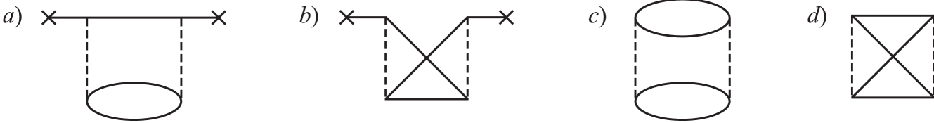
Figure 1: Second-order diagrams for the corrections to the temperature scattering matrix in the field representation.

We now calculate the second-order correction term to the temperature scattering matrix which, according to (83), determines a correction to the thermodynamic potential. Each of the first and second terms in (89) corresponds to two nonequivalent diagrams in Fig. 1. The second-order contribution to the temperature scattering matrix is determined by the formula

$$\begin{array}[]{ll}\displaystyle{\langle\sigma_{2}(\beta)\rangle_{0c}=\frac{g^{2}}{2!}\Bigg{\{}\frac{(-1)}{2^{2}}\int\!\!d1^{\prime}d2^{\prime}d1^{\prime\prime}d2^{\prime\prime}\times\vspace{2mm}}\\ \displaystyle{\hskip 5.69054pt\times\,\tilde{U}(1^{\prime},2^{\prime})\,\tilde{U}(1^{\prime\prime},2^{\prime\prime})\,\chi(1^{\prime})\,\chi(1^{\prime\prime})\,\times\vspace{2mm}}\\ \displaystyle{\hskip 5.69054pt\times\Big{[}2\,G^{(0)}\!(2^{\prime},2^{\prime\prime})\,G^{(0)}\!(\bar{2}^{\prime},\bar{2}^{\prime\prime})\,G^{(0)}\!(\bar{1}^{\prime},\bar{1}^{\prime\prime})+\vspace{2mm}}\\ \displaystyle{\hskip 11.38109pt+4\,G^{(0)}\!(2^{\prime},2^{\prime\prime})\,G^{(0)}\!(\bar{2}^{\prime},\bar{1}^{\prime\prime})\,G^{(0)}\!(\bar{1}^{\prime},\bar{2}^{\prime\prime})\Big{]}+\vspace{2mm}}\\ \displaystyle{\hskip 5.69054pt+\frac{1}{8^{2}}\int\!\!d1^{\prime}d2^{\prime}d1^{\prime\prime}d2^{\prime\prime}\,\tilde{U}(1^{\prime},2^{\prime})\,\tilde{U}(1^{\prime\prime},2^{\prime\prime})\,\times\vspace{2mm}}\\ \displaystyle{\hskip 5.69054pt\times\Big{[}8\,G^{(0)}\!(1^{\prime},1^{\prime\prime})\,G^{(0)}\!(2^{\prime},2^{\prime\prime})\,G^{(0)}\!(\bar{2}^{\prime},\bar{2}^{\prime\prime})\,G^{(0)}\!(\bar{1}^{\prime},\bar{1}^{\prime\prime})+\vspace{2mm}}\\ \displaystyle{\hskip 5.69054pt+16\,G^{(0)}\!(1^{\prime},1^{\prime\prime})\,G^{(0)}\!(2^{\prime},2^{\prime\prime})\,G^{(0)}\!(\bar{2}^{\prime},\bar{1}^{\prime\prime})\,G^{(0)}\!(\bar{1}^{\prime},\bar{2}^{\prime\prime})\Big{]}\Bigg{\}}.}\end{array}$$ (92)

We now turn to the consideration of the corrections to GFs. First, we consider the first order of perturbation theory. In this order, the corrections to the one- and two-point GFs are equal to zero. The corrections to the three- and four-point GFs are described by the diagrams $(a)$ and $(b)$, respectively, in Fig. 2. In these diagrams, the indices of the outer lines should be arranged by all nonequivalent means; in our case, the number of such configurations turns out to be three per each diagram. Analytically, the correction term to the three-point GF has the form

$$\begin{array}[]{ll}\displaystyle{G^{(1)}\!(1,2,3)=-gi^{3}\!\int\!\!d1^{\prime}d2^{\prime}\,\tilde{U}(1^{\prime},2^{\prime})\,\chi(1^{\prime})\,\times\vspace{2mm}}\\ \displaystyle{\hskip 8.53581pt\times\Big{[}G^{(0)}\!(1,2^{\prime})\,G^{(0)}\!(2,\bar{2}^{\prime})\,G^{(0)}\!(3,\bar{1}^{\prime})+\vspace{2mm}}\\ \displaystyle{\hskip 14.22636pt+G^{(0)}\!(1,2^{\prime})\,G^{(0)}\!(2,\bar{1}^{\prime})\,G^{(0)}\!(3,\bar{2}^{\prime})+\vspace{2mm}}\\ \displaystyle{\hskip 14.22636pt+G^{(0)}\!(1,\bar{1}^{\prime})\,G^{(0)}\!(2,2^{\prime})\,G^{(0)}\!(3,\bar{2}^{\prime})\Big{]},}\end{array}$$ (93)

whereas that to the four-point one reads

$$\begin{array}[]{ll}\displaystyle{G^{(1)}\!(1,2,3,4)=-gi^{4}\!\int\!\!d1^{\prime}d2^{\prime}\,\tilde{U}(1^{\prime},2^{\prime})\,\times\vspace{2mm}}\\ \displaystyle{\hskip 8.53581pt\times\Big{[}G^{(0)}\!(1,1^{\prime})\,G^{(0)}\!(2,2^{\prime})\,G^{(0)}\!(3,\bar{2}^{\prime})\,G^{(0)}\!(4,\bar{1}^{\prime})+\vspace{2mm}}\\ \displaystyle{\hskip 14.22636pt+G^{(0)}\!(1,1^{\prime})\,G^{(0)}\!(2,2^{\prime})\,G^{(0)}\!(4,\bar{2}^{\prime})\,G^{(0)}\!(3,\bar{1}^{\prime})+\vspace{2mm}}\\ \displaystyle{\hskip 14.22636pt+G^{(0)}\!(1,1^{\prime})\,G^{(0)}\!(2,\bar{1}^{\prime})\,G^{(0)}\!(3,2^{\prime})\,G^{(0)}\!(4,\bar{2}^{\prime})\Big{]}.}\end{array}$$ (94)

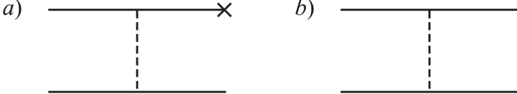
Figure 2: First-order diagrams for the corrections to the three-point (a) and four-point (b) GFs in the field representation.

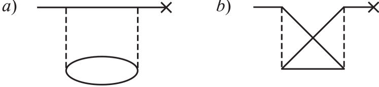
Figure 3: First-order diagrams for the corrections to the three-point (a) and four-point (b) GFs in the field representation.

Consider the second order corrections. The corrections to the one-point GF are described by the two diagrams in Fig. 3 and have the forms

$$\begin{array}[]{ll}\displaystyle{G^{(2)}\!(1)=ig^{2}\!\int\!\!d1^{\prime}d2^{\prime}d1^{\prime\prime}d2^{\prime\prime}\,\tilde{U}(1^{\prime},2^{\prime})\,\tilde{U}(1^{\prime\prime},2^{\prime\prime})\,\chi(1^{\prime})\,\times\vspace{2mm}}\\ \displaystyle{\hskip 8.53581pt\times\bigg{[}\frac{1}{2}\,G^{(0)}\!(1,1^{\prime\prime})\,G^{(0)}\!(2^{\prime},2^{\prime\prime})\,G^{(0)}\!(\bar{2}^{\prime},\bar{2}^{\prime\prime})\,G^{(0)}\!(\bar{1}^{\prime},\bar{1}^{\prime\prime})+\vspace{2mm}}\\ \displaystyle{\hskip 22.76219pt+G^{(0)}\!(1,1^{\prime\prime})\,G^{(0)}\!(2^{\prime},2^{\prime\prime})\,G^{(0)}\!(\bar{2}^{\prime},\bar{1}^{\prime\prime})\,G^{(0)}\!(\bar{1}^{\prime},\bar{2}^{\prime\prime})\bigg{]}.}\end{array}$$ (95)

The second-order corrections to the higher order GFs can be constructed in a similar manner.

The analysis of the formulae obtained shows that the diagram, which describes the $n$-order contribution to the $L$-point GF, contains:

(a) $2n$ vertices connected in pairs by dashed lines (interaction lines), each of which corresponds to the multiplier $\tilde{U}\!(1^{\prime},2^{\prime})$;

(b) the internal solid lines (of the Green type), which correspond to the multiplier $G^{(0)}\!(1^{\prime},1^{\prime\prime})$ and connect the vertices of different dashed lines. We note that the Green’s line cannot connect the vertices of the same dashed line. In particular, its beginning and end cannot belong to the same vertex;

(c) $L$ outer Green’s lines, for which only one end is connected with the interaction line vertex;

(d) the Bose condensate lines (with the sign “$\times$”) which are connected only with one vertex of a dashed line (the other end of the interaction line cannot be connected with one more Bose condensate line). The diagrams with the even number of outer Greens’s lines ($L=2S$) contain the even number of Bose condensate lines. The diagrams with the odd number of outer Greens’s lines ($L=2S+1$) contain the odd number of Bose condensate lines.

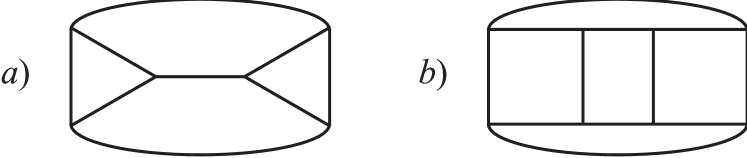
Figure 4: Second-order diagrams for the corrections to the temperature scattering matrix in the quasiparticle representation.

Thus, to calculate the $n$-order contribution to the $L$-point GF, it is necessary:

(a) to depict all the topologically nonequivalent $n$-order diagrams, i.e. those ones which don’t turn into one another under the permutations of the vertex indices of interaction lines;

(b) to associate the lines with their analytical expressions;

(c) to integrate over all the indices corresponding to the vertices of interactions lines (the integration also includes the summation over all the discrete indices);

(d) to perform such procedures: the index of the vertex of the interaction line, which is included either in two GFs (when two Green’s lines converge into a vertex) or in the GF and the Bose condensate function (when the GF and the Bose condensate line converge into a vertex), has to be written once without the overbar, and for the second time with the overbar;

(e) to put the multiplier $(-1)^{n}/2^{k}$ before the expression obtained, where $n$ is the diagram order and $k$ is the number of closed Green’s lines in the diagram.

For the practical utilization of the diagram technique, the frequency representation turns out to be more suitable. The Fourier component of the $L$-point GF is handy to define as

$$\begin{array}[]{ll}\displaystyle{G(1,2,\ldots L;\omega_{1},\omega_{2},\ldots\omega_{L})=\vspace{2mm}}\\ \displaystyle{=\!\beta\Delta(\omega_{1}+\omega_{2}+\ldots+\omega_{L})G(1,2,\ldots L;\omega_{1},\omega_{2},\ldots\omega_{L-1}),}\end{array}$$ (96)

where

$$\begin{array}[]{ll}\displaystyle{G(1,2,\ldots L;\omega_{1},\omega_{2},\ldots\omega_{L-1})=\vspace{2mm}}\\ \displaystyle{\hskip 8.53581pt=\frac{1}{2^{L-1}}\int_{-\beta}^{\beta}\!d(\tau_{1}-\tau_{2})\ldots\int_{-\beta}^{\beta}\!d(\tau_{L-1}-\tau_{L})\times\vspace{2mm}}\\ \displaystyle{\hskip 8.53581pt\times\,G(1,2,\ldots L;\tau_{1}-\tau_{2},\ldots\tau_{L-1}-\tau_{L})\times\vspace{2mm}}\\ \displaystyle{\hskip 8.53581pt\times\,e^{i\omega_{1}(\tau_{1}-\tau_{2})+\ldots+i\omega_{L-1}(\tau_{L-1}-\tau_{L})}.}\end{array}$$ (97)

In this case, in order to calculate the $L$-point GF, the rules of the diagram technique have to undergo the following modifications:

(a) every Green’s line is associated with the Fourier component $G^{(0)}\!(1,2;\omega_{n})$;

(b) every dashed line is associated with the potential $\underline{\tilde{U}}(1,2)=U(x_{1},x_{2})(\delta_{\alpha_{1}\alpha_{2}}+\delta_{\alpha_{1}\bar{\alpha}_{2}})$;

(c) every dashed interaction line is associated with the multiplier $\Delta(\omega_{1}^{\prime}+\omega_{2}^{\prime}+\omega_{3}^{\prime}+\omega_{4}^{\prime})$ or $\Delta(\omega_{1}^{\prime}+\omega_{2}^{\prime}+\omega_{3}^{\prime})$ (in the case where one of the lines converging into a vertex is a Bose condensate line). Here, $\omega_{k}^{\prime}$ are the frequencies which correspond to the Green’s lines converging at the vertices of a given dashed line. In this case, for all such GFs, the vertex indices for the interaction lines have to be put either all at the first place or all at the second place. If the order of indices is changed for a GF line, a sign is to be changed in the above multipliers $\Delta$;

(d) the additional multiplier $T^{n}\beta\Delta(\omega_{1}+\omega_{2}+\ldots+\omega_{L})$, where $n$ is the order of the diagram, emerges before the expression.

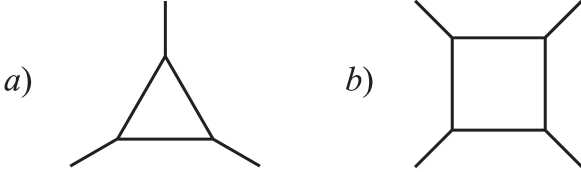
Figure 5: Second-order diagrams for the corrections to the temperature scattering matrix in the quasiparticle representation.

Finally, we formulate the rules of the diagram technique in the quasiparticle representation. We associate the matrix elements (74) with a square and a triangle,

$$\begin{array}[]{ll}\displaystyle{\tilde{U}_{\bar{1}\bar{2}\bar{3}\bar{4}}\hskip 5.69054pt\textrm{---}\hskip 5.69054pt\scalebox{0.65}[0.65]{\includegraphics[bb=28 490 85 510]{IV1.eps}},\quad\tilde{U}_{\bar{1}\bar{2}\bar{3}}\hskip 5.69054pt\textrm{---}\hskip 5.69054pt\scalebox{0.65}[0.65]{\includegraphics[bb=30 489 193 515]{IV2.eps}},\vspace{2.5mm}}\end{array}$$

and the solid Green’s line with $G^{(0)}\!(i\tau,i^{\prime}\tau^{\prime})$. All the indices of the square or the triangle correspond to the same time parameter $\tau$. We recall that the wave function of the Bose condensate is contained in the matrix element with three indices (in the triangle). The $n$-order diagrams consist of $n$ squares and triangles, whose vertices are connected by Green’s lines by all possible nonequivalent means. To calculate the $n$-order contribution, we have to depict all topologically nonequivalent diagrams, relate their elements to analytic expressions, and integrate over the indices of the square and triangle vertices, as well as the corresponding time parameters.

For the sake of illustration, we note that the second-order contribution to the temperature scattering matrix is determined by two diagrams in Fig. 4, and the first-order contribution to the three-point $(a)$ and four-point $(b)$ GFs – by the diagrams shown in Fig. 5. In the quasiparticle representation, the diagrams are simpler but the matrix elements of the interaction are much more complex. As in the usual diagram technique, the block summation of diagrams is allowable.

8. For the approach we developed, the self-energy and vertex functions can be introduced, and the Dyson equations connecting these functions can be written. The system of equations for the one-point and two-point has the form

$$\begin{array}[]{ll}\displaystyle{\int\!\!d2\Big{[}\Omega(1,\bar{2})+g\,\Theta(1,\bar{2})\Big{]}G(2)\,+\vspace{2mm}}\\ \displaystyle{\hskip 8.53581pt+\,g\int\!\!d2d3\Big{[}V^{(0)}(1,2,\bar{3})+\Lambda(1,2,\bar{3})\Big{]}G(3,2)=\vspace{2mm}}\\ \displaystyle{\hskip 8.53581pt=g\int\!\!d2d3\,V^{(0)}\!(1,2,\bar{3})\,G^{(0)}\!(3,2),}\end{array}$$ (98)

$$\begin{array}[]{ll}\displaystyle{\frac{\partial G(1,2)}{\partial\tau_{1}}+\sigma_{\bar{\alpha}_{1}}\int\!\!d3\Big{[}\Omega(1,\bar{3})+g\,\Theta(1,\bar{3})\,+\vspace{2mm}}\\ \displaystyle{\hskip 8.53581pt+\,g\Sigma(1,\bar{3})\Big{]}G(3,2)+g\sigma_{\bar{\alpha}_{1}}Z(1)\,G(2)=-\sigma_{\bar{\alpha}_{1}}\delta(1-\bar{2}),}\end{array}$$ (99)

where $1=(x_{1},\tau_{1},\alpha_{1})$ and $\bar{1}=(x_{1},\tau_{1},\bar{\alpha}_{1})$. In Eqs. (98) and (99), the designations

$$\begin{array}[]{ll}\displaystyle{\Theta(1,2)=\tilde{U}(1,2)\Big{[}G^{(0)}\!(1,2)-G(1,2)\Big{]}+\vspace{2mm}}\\ \displaystyle{\hskip 8.53581pt+\frac{1}{2}\,\delta(1-\bar{2})\int\!\!d3\,\tilde{U}(1,3)\Big{[}G^{(0)}\!(3,\bar{3})-G(3,\bar{3})\Big{]},}\end{array}$$ (100)

$$\begin{array}[]{ll}\displaystyle{\Lambda(1,2,3)=\vspace{2mm}}\\ \displaystyle{\hskip 8.53581pt=-\frac{1}{2}\,\tilde{U}(1,2)\int\!\!d1^{\prime}d2^{\prime}\,\Gamma(1^{\prime},2^{\prime},3)\,G(\bar{1}^{\prime},1)\,G(\bar{2}^{\prime},2),}\end{array}$$ (101)

$$\begin{array}[]{ll}\displaystyle{Z(1)=\int\!\!d3d4\,V^{(0)}\!(1,3,\bar{4})\Big{[}G(\bar{3},4)-G^{(0)}\!(\bar{3},4)\Big{]},}\end{array}$$ (102)

$$\begin{array}[]{ll}\displaystyle{\Sigma(1,3)=\int\!\!d4\Big{[}V^{(0)}\!(1,3,\bar{4})+V^{(0)}\!(1,4,\bar{3})\Big{]}G(4)+\vspace{2mm}}\\ \displaystyle{+\!\int\!\!d1^{\prime}d2^{\prime}d3^{\prime}d4\,V^{(0)}\!(1,3^{\prime},\bar{4})\,\Gamma(1^{\prime},2^{\prime},\bar{3})\,G(\bar{1}^{\prime},3^{\prime})\,G(\bar{2}^{\prime},4)-\vspace{2mm}}\\ \displaystyle{-\frac{1}{2}\!\int\!\!d1^{\prime}d2^{\prime}d3^{\prime}d4\,\tilde{U}(1,4)\,\Gamma(1^{\prime},2^{\prime},3^{\prime},\bar{3})\times\vspace{2mm}}\\ \displaystyle{\hskip 128.0374pt\times G(\bar{1}^{\prime},1)\,G(\bar{2}^{\prime},\bar{4})\,G(\bar{3}^{\prime},4),}\end{array}$$ (103)

$$\begin{array}[]{ll}\displaystyle{V^{(0)}\!(1,2,3)=\vspace{2mm}}\\ \displaystyle{\hskip 8.53581pt=-\frac{i}{2}\,\tilde{U}(1,2)\big{[}2\chi(2)\,\delta(1-3)+\chi(1)\,\delta(\bar{2}-3)\big{]}}\end{array}$$ (104)

are used. The three-point and four-point vertex functions read

$$\begin{array}[]{ll}\displaystyle{G(1,2,3)=G(1,2)\,G(3)+G(1,3)\,G(2)+G(2,3)\,G(1)+\vspace{2mm}}\\ \displaystyle{\hskip 8.53581pt+\int\!\!d1^{\prime}d2^{\prime}d3^{\prime}\,\Gamma(1,2^{\prime},3^{\prime})\,G(\bar{1}^{\prime},1)\,G(\bar{2}^{\prime},2)\,G(\bar{3}^{\prime},3),}\end{array}$$

$$\begin{array}[]{ll}\displaystyle{G(1,2,3,4)=\vspace{2mm}}\\ \displaystyle{\hskip 8.53581pt=G(1,2)\,G(3,4)+G(1,3)\,G(2,4)+G(1,4)\,G(2,3)+\vspace{2mm}}\\ \displaystyle{\hskip 8.53581pt+\int\!\!d1^{\prime}d2^{\prime}d3^{\prime}d4^{\prime}\,\Gamma(1,2^{\prime},3^{\prime},4^{\prime})\times\vspace{2mm}}\\ \displaystyle{\hskip 88.20354pt\times\,G(\bar{1}^{\prime},1)\,G(\bar{2}^{\prime},2)\,G(\bar{3}^{\prime},3)\,G(\bar{4}^{\prime},4).}\end{array}$$ (105)

The one-point GF is associated with the self-energy functions by the relation

$$\begin{array}[]{ll}\displaystyle{G(1,2)=G^{(0)}\!(1,2)+g\!\int\!\!d3d4\,G^{(0)}\!(1,\bar{3})\,\tilde{\Sigma}(3,\bar{4})\,G(4,2)+\vspace{2mm}}\\ \displaystyle{\hskip 8.53581pt+g\!\int\!\!d3\,G^{(0)}\!(1,\bar{3})\,Z(3)\,G(2),}\end{array}$$ (106)

where $\tilde{\Sigma}(1,2)=\Theta(1,2)+\Sigma(1,2).$ Expressions (101) and (103) describe the relation of the self-energy functions $\Lambda(1,2,3)$ and $\Sigma(1,3)$, on the one hand, to the vertex functions $\Gamma(1,2,3)$ and $\Gamma(1,2,3,4)$, on the other hand. These expressions are the analogs of the Dyson equations for the many-particle Bose systems. As is seen, in the Bose systems with the single-particle Bose condensate, the additional vertex function $V^{(0)}\!(1,2,3)$, which originates from both the interaction potential and the wave function of the Bose condensate, emerges. We pay attention to the fact that the system of equations (98) and (99), as well as the subsequent relations, essentially differ from the Dyson equations obtained in the Belyaev’s approach Belyaev . Contrary to the case described in Belyaev , this systems contains both the two-point and one-point (condensate) GFs. The different structure of the Dyson equations turns out to be very important. In particular, it is on investigation of the Dyson equations that some general statements about the character of the spectrum of excitations in the Bose systems are based Bogolyubov3 .

It is known AGD that the poles of a vertex function determine the dispersion law for the collective excitations in a many-particle system. This spectrum cannot be obtained as a result of the calculation of the vertex function in any finite order of perturbation theory. The four-point vertex function can be represented as the sum of two functions, $\Gamma=\Gamma_{1}+\Gamma_{2}$. One of these functions, $\Gamma_{1}$ is the sum of infinite “stepwise” series, whose terms are compact quadrilaterals $\Gamma_{k}$ connected by the pairs of Green’s lines which correspond to exact GFs. The second function, $\Gamma_{2}$, contains all diagrams which did not enter into $\Gamma_{1}$. Just the function $\Gamma_{1}$ gives rise to the appearance of the pole which corresponds to collective excitations. It satisfies the relation

$$\begin{array}[]{ll}\displaystyle{\Gamma^{(1)}\!(1,2,3,4)=\Gamma_{k}(1,2,3,4)\,+\vspace{2mm}}\\ \displaystyle{\hskip 5.69054pt+\!\int\!\!d5d6d7d8\,\Gamma_{k}(1,2,5,6)\,G(5,7)\,G(6,8)\,\Gamma^{(1)}\!(7,8,3,4).}\end{array}$$ (107)

We note that the method of calculation of the dispersion law for zero-sound collective excitations with the help of summation of the infinite series of “stepwise” diagrams is well known in the theory of Fermi systems AGD . An analogous situation occurs also in Bose systems. The assumption that the interparticle interaction is weak makes it possible to substitute the exact GFs in (107) by their values in the zero approximation. This allows us to write the equation which determines the dispersion law for the collective excitations:

$$\begin{array}[]{ll}\displaystyle{1=\frac{U_{0}}{V}\,\sum_{{\bf p}}\frac{f(\varepsilon_{{\bf p}})-f(\varepsilon_{{\bf p}+{\bf k}})}{\omega-\varepsilon_{{\bf p}+{\bf k}}+\varepsilon_{{\bf p}}}.}\end{array}$$ (108)

Here, $U_{0}$ is the interaction constant, $V$ is the volume, $\varepsilon_{{\bf k}}$ is the dispersion law for a single-particle excitation, and $f(\varepsilon_{{\bf k}})$ is the Bose distribution function. Relation (108) yields the sound dispersion law for the collective excitations, whose velocity $c_{0}=\big{(}U_{0}n/m\big{)}^{1/2}$ ($m$ is the particle mass) doesn’t depend on temperature and is determined by both the particle number density $n$ and interaction constant and is the same in the normal and superfluid phases. It is the collective excitations that form the linear part of the spectrum in many-particle Bose systems. The independence of the linear part of the spectrum from temperature (outside the hydrodynamic area) is confirmed in the experiments on the inelastic scattering of slow neutrons in liquid ⁴He BKKP ; Kozlov .

In this work, we have proposed a quantum-field method for the theoretical description of many-particle Bose systems which are in the states with broken symmetry. This approach is based on the choice of the generalized model of self-consistent field as the initial approximation. Such a choice of the basic approximation, which is more realistic in comparison with the case of the model of ideal Bose gas, makes it possible to avoid the difficulties emerging in the available theory PS ; N and provides the opportunity to investigate the spatially inhomogeneous states and, in particular, the states with superfluid flows. In the basic approximation, the spectrum of single-particle excitations of a Bose system is calculated in the SCF model, whereas the spectrum of collective excitations is determined by the poles of three- and four-point GFs or vertex functions. The approach proposed does not contain any assumptions, is based only on the general principles of quantum mechanics and statistical physics, and is equally applicable for the description of Fermi Poluektov3 ; Poluektov4 and Bose systems.

References

(1)
A.A. Abrikosov, L.P. Gor’kov, I.E. Dzyaloshinskii, Methods of
quantum field theory in statistical physics. – New York: Dover,
1963.
(16)
M.Yu. Kovalevskii and S.V. Peletminskii, Statistical mechanics of
quantum fluids and crystals. – Moscow: Fizmatlit, 2006 (in
Russian).
(17)
N.N. Bogolyubov, Uspekhi Fiz. Nauk 67, 549 (1959).
(18)
P.G. de Gennes, Superconductivity of metals and alloys. – Reading,
MA: Addison-Wesley, 1999.
(19)
J. Bardeen, L. Cooper, J. Schrieffer, Phys. Rev. 108,
1175 (1957).
(20)
N.N. Bogolyubov, V.V. Tolmachev, D.V. Shirkov, A new method in
the theory of superconductivity. – New York: Consultants Bureau,
1959 (Izdat. AN SSSR, Moscow, 1958, in Russian).
(21)
M. Girardeau and R. Arnowitt, Phys. Rev. 113, 755 (1959).