Nambu–Goldstone mesons in strong magnetic field

Abstract

We study the $q\bar{q}$ structure embedded in chiral mesons in response to external magnetic fields (m.f.), using the chiral Lagrangian with $q\bar{q}$ degrees of freedom derived earlier. We show that GMOR relations hold true for neutral chiral mesons, while they are violated for the charged ones for $eB>\sigma=0.2$ GeV². The standard chiral perturbation theory also fails in this region. Masses of $\pi^{+}$ and $\pi^{0}$ mesons are calculated and compared to lattice data.

1 Introduction

Chiral Lagrangians introduced to clarify the dynamics of Nambu–Goldstone mesons have created a new selfconsistent formalism [1] prior to the emergence of QCD.

One of the basic conceptual relations in QCD is the relation of the purely chiral particles – the Nambu–Goldstone (NG) mesons – to all other QCD states, which are mostly nonchiral. It other words one can define this as a connection of Nambu–Goldstone to ordinary states, which can be called pure confinement or the flux-tube states. The models treating most states in the phenomenological chiral-like Lagrangians are now numerous, but unfortunately they do not clarify this chiral – confinement connection.

In [2, 3, 4, 5] one of the authors suggested a way of derivation the chiral Nambu–Goldstone spectrum from the QCD Lagrangian, where the basic chiral relations: chiral condensate, GMOR relation and expressions for $m^{2}_{\pi},f^{2}_{\pi}$ are derived in terms of confinement (flux-tube) spectrum in the PS isovector channel. The latter is calculated from the Relativistic Hamiltonian in the framework of Field-Correlator Method (FCM) [6] in terms of the basic input: current quark masses $m_{i}$, string tension $\sigma$ and $\alpha_{s}$, and the FCM provides a good description of the QCD spectrum in all channels and for all masses $m_{i}$, except for NG mesons: $\pi,K,\eta$.

The connection of NG and flux-tube mesons [2, 3, 4, 5] described above, which may be called the chiral-confinement relations (CCR), allows to express NG meson masses, wave functions and quark decay constants in terms of the same basic input and in this way completes the theory. One should note, that in the CCR one calculates not only ground states, but also excited NG states [4, 5] and, moreover, one can study how chiral properties fade away with growing quark current masses $m_{i}$ [7].

Recently a wide interest has occurred in the literature in the effects, which can be produced in hadron dynamics due to strong external magnetic fields (m.f.) [8]. In particular, strong m.f. are expected in neutron stars [9], early universe [10], heavy ion collisions [11] and possibly m.f. can produce strong reconstruction of the vacuum [12].

From the theoretical point of view, strong m.f. play the role of crucial test of the dynamics used in the model. For the QCD as a strong interaction theory one must use the relativistic dynamical formalism, incorporating confinement and perturbative gluon exchanges, producing all effects of strong decays. This is naturally imbedded in the FCM formalism, based on the QCD path integral, where one derives the relativistic Hamiltonian (RH) for the $q\bar{q},3q$ etc. states.

The inclusion of m.f. is done automatically in the RH, and the first results for the masses were already obtained in [13], while the important role of color Coulomb interaction in strong m.f. was studied in [14], and magnetic moments of mesons in [15].

Of special interest is the influence of m.f. on chiral dynamics, and in this way one can check that the CCR sustain their reliability in the presence of m.f. [16]. On the lattice several analysis were done [17, 18, 19] on chiral dynamics in m.f., e.g. the dependence of $\pi^{+}$ mass and chiral condensate on m.f. was done in unquenched QCD with physical pion mass [20]. These results were compared with the CCR prediction for the $\langle\bar{u}u\rangle$ and $\langle\bar{d}d\rangle$ dependence on m.f. and a good agreement was found in [16].

On thee other hand, this dependence found on the lattice was compared in [20] with the what one expects from the chiral theory, and a strong disagreement was found for $eB>0.2$ GeV². This implied that the standard chiral theory [4], which lacks quark degrees of freedom, is unable to be a good working tool for distances less than 0.5 fm.

In this paper we study the m.f. dependence of the NG spectrum, which follows from CCR. The latter expresses the NG masses through nonchiral PS isovector states, and we approximate several lowest states, which give the dominant contribution to CCR, in their m.f. dependence and obtain NG masses.

One of the most important result of this paper is the violation of GMOR relations and of the standard chiral formalism in the m.f. There appear additional terms in the NG Lagrangian, proportional to m.f., which disclose the internal quark-antiquark structure of NG mesons, not accounted for in the standard chiral formalism of [1]. As a result the dependence of NG meson mass on m.f. contains new terms, which do not vanish in the chiral limit $m_{q}=0$. This behavior is supported by lattice data [20] for the behavior of the $\pi^{+}$ mass in m.f.

In what follows we introduce first in section 2 RH for neutral and charged $q\bar{q}$ states in m.f., in section 3 we write down the basic equations of CCR and generalize them to the case of nonzero m.f. Section 4 is devoted to the calculation of NG states and in section 5 results are compared with chiral perturbation theory and lattice data.

2 Relativistic Hamiltonian for mesons in strong magnetic field

The RH for the $q\bar{q}$ system in m.f. was derived recently in [13, 21] from the path integral in QCD and we follow these notations and definitions.

$$H=H_{0}+H_{\sigma}+W,$$ (1)

where

$$H_{0}=\sum^{2}_{i=1}\frac{\left(\mbox{\boldmath${\rm p}$}^{(i)}-\frac{e_{i}}{2}(\mbox{\boldmath${\rm B}$}\times\mbox{\boldmath${\rm z}$}^{(i)})\right)^{2}+m^{2}_{i}+\omega^{2}_{i}}{2\omega_{i}},$$ (2)

$$H_{\sigma}=-\frac{e_{1}\mbox{\boldmath${\rm\sigma}$}_{1}\mbox{\boldmath${\rm B}$}}{2\omega_{1}}-\frac{e_{2}\mbox{\boldmath${\rm\sigma}$}_{2}\mbox{\boldmath${\rm B}$}}{2\omega_{2}},$$ (3)

$$W=V_{\rm conf}+V_{\rm Coul}+V_{SD}+\Delta M_{ss}.$$ (4)

One defines $\omega_{i}\to\omega_{i}^{(0)}$ from the extremum values of eigenvalues of the operator $\bar{H}$

$$H_{0}+H_{\sigma}+V_{conf}=\bar{H};~{}~{}\bar{H}\Psi=M_{n}^{(0)}\Psi,$$ (5)

$$\left.\frac{\partial M_{n}^{(0)}(\omega_{1}\omega_{2})}{\partial\omega_{1}}\right|_{\omega_{i}=\omega_{i}^{(0)}}=0,~{}~{}i=1,2.$$ (6)

We now treat $H_{0}$ and try to separate c.m. and relative motion

$$\mbox{\boldmath${\rm R}$}=\frac{\omega_{1}\mbox{\boldmath${\rm z}$}^{(1)}+\omega_{2}\mbox{\boldmath${\rm z}$}^{(2)}}{\omega_{1}+\omega_{2}},~{}~{}\mbox{\boldmath${\rm\eta}$}=\mbox{\boldmath${\rm z}$}^{(1)}-\mbox{\boldmath${\rm z}$}^{(2)},$$ (7)

For two-body systems $q\bar{q}$ the c.m. and relative motion can be separated in two cases:

a)$e_{1}+e_{2}=0,$ neutral case:

b) $e_{1}=e_{2},~{}m_{1}=m_{2},~{}\omega_{1}=\omega_{2}$.

We shall consider both cases below.

In case a) one introduces the so-called “phase factor”,

$$\Psi(\mbox{\boldmath${\rm\eta}$},\mbox{\boldmath${\rm R}$})=\exp(i\Gamma)\varphi(\mbox{\boldmath${\rm\eta}$},\mbox{\boldmath${\rm R}$}),$$ (8)

$$\Gamma=\mathbf{P}\mathbf{R}-\frac{\bar{e}}{2}(\mbox{\boldmath${\rm B}$}\times\mbox{\boldmath${\rm\eta}$})\mbox{\boldmath${\rm R}$},~{}~{}\bar{e}=\frac{e_{1}-e_{2}}{2},$$ (9)

and defines a new operator $H^{\prime}_{0}$ from the relation

$$H_{0}\Psi=\exp(i\Gamma)H^{\prime}_{0}\varphi,$$ (10)

$$H^{\prime}_{0}=\frac{1}{2\tilde{\omega}}\left(-\frac{\partial^{2}}{\partial\mbox{\boldmath${\rm\eta}$}^{2}}+\frac{e^{2}}{4}(\mbox{\boldmath${\rm B}$}\times\mbox{\boldmath${\rm\eta}$})^{2}\right)+\sum^{2}_{i=1}\frac{m^{2}_{i}+\omega^{2}_{i}}{2\omega_{i}},$$ (11)

At this point it is convenient to replace linear confinement by the quadratic one, with adjustable coefficient $\gamma$, which yields a deviation $\mathrel{\mathchoice{\lower 3.6pt\vbox{\halign{$\mathsurround=0pt\displaystyle\hfil#\hfil$\cr<\crcr\sim\crcr}}}{\lower 3.6pt\vbox{\halign{$\mathsurround=0pt\textstyle\hfil#\hfil$\cr<\crcr\sim\crcr}}}{\lower 3.6pt\vbox{\halign{$\mathsurround=0pt\scriptstyle\hfil#\hfil$\cr<\crcr\sim\crcr}}}{\lower 3.6pt\vbox{\halign{$\mathsurround=0pt\scriptscriptstyle\hfil#\hfil$\cr<\crcr\sim\crcr}}}}5\%$ in resulting masses,

$$V_{\rm conf}=\sigma\eta\to\tilde{V}_{\rm conf}=\frac{\sigma}{2}\left(\frac{\eta^{2}}{\gamma}+\gamma\right)$$ (12)

and now the average mass $M_{n}$ is the eigenvalue of the operator $\bar{H}^{\prime}$

$$\bar{H}^{\prime}=H^{\prime}_{0}+H_{\sigma}+\tilde{V}_{\rm conf};~{}~{}\bar{H}^{\prime}\varphi=\bar{M}_{n}\varphi,$$ (13)

defines the extremal values of $(\omega_{1},\omega_{2},\gamma)$

$$\left.\frac{\partial\bar{M}_{n}(\omega_{1},\omega_{2},\gamma)}{\partial\omega_{1}}\right|_{\omega_{1}=\omega_{1}^{(0)}}=\left.\frac{\partial\bar{M}_{n}}{\partial\omega_{2}}\right|_{(\omega_{2}=\omega_{2}^{(0)}}=\left.\frac{\partial\bar{M}_{n}}{\partial\gamma}\right|_{\gamma=\gamma_{0}}=0.$$ (14)

The resulting form of $\bar{M}_{n}^{(0)}=M_{n}(\omega_{1}^{(0)},\omega_{2}^{(0)},\gamma_{0})$ defines the total mass of the meson,

$$M_{n}=\bar{M}_{n}^{(0)}+\Delta M_{\rm coul}+\Delta M_{SE}+\Delta M_{ss}.$$ (15)

The form of $\bar{M}_{n}$ (prior to stationary point insertions) is

$$\bar{M}_{n}=\varepsilon_{n_{\bot},n_{z}}+\frac{m_{1}^{2}+\omega^{2}_{1}-e\mbox{\boldmath${\rm B}$}\mbox{\boldmath${\rm\sigma}$}_{1}}{2\omega_{1}}+\frac{m_{2}^{2}+\omega^{2}_{2}+e\mbox{\boldmath${\rm B}$}\mbox{\boldmath${\rm\sigma}$}_{2}}{2\omega_{2}},$$ (16)

where

$$\varepsilon_{n_{\bot},n_{z}}=\frac{1}{2\tilde{\omega}}\left[\sqrt{e^{2}B^{2}+\frac{4\sigma\tilde{\omega}}{\gamma}}(2n_{\bot}+1)+\sqrt{\frac{4\sigma\tilde{\omega}}{\gamma}}\left(n_{z}+\frac{1}{2}\right)\right]+\frac{\gamma\sigma}{2}.$$ (17)

The retaining three terms in (15) are defined as follows:

1) $\Delta M_{\rm Coul}=\langle V_{\rm Coul}\rangle$, where averaging is done with wave functions $\varphi_{n}$ defined in (13), and $V_{\rm Coul}$ is the OGE interaction $V_{\rm Coul}(\mbox{\boldmath${\rm q}$})=\frac{-16\pi\alpha_{s}}{3\mbox{\boldmath${\rm q}$}^{2}}$, and at large m.f. $\mbox{\boldmath${\rm q}$}^{2}$ is augmented by the $(q\bar{q})$ loop contribution, see details in [14].

2), 3) $\Delta M_{SE}$ and $\Delta M_{ss}$ are given in [13] and we rewrite those in the Appendix.

We now turn to the case b), and consider two-body system with equal charges and masses. It is clear, that relativistic charged pions and kaons contain charges $e_{1}=\frac{2}{3}e,e_{2}=\frac{1}{3}e$, in contrast to the case b), however the main new feature in the case b) is the contribution of the c.m. motion in m.f. to the total mass and this is pertinent also to the realistic case, the difference between the case b) and the realistic case can possibly be treated in a perturbative manner. As it is clear from (8), (9), the phase factor $\Gamma$ is not necessary in the case b), and one obtains the Hamiltonian as in Eq.(34), we also put below $\omega_{1}=\omega_{2}=\omega,e_{1}=e_{2}=e.$

$$H=\frac{P^{2}}{4\omega}-\frac{e(\mbox{\boldmath${\rm P}$}(\mbox{\boldmath${\rm B}$}\times\mbox{\boldmath${\rm R}$}))}{2\omega}+\frac{e^{2}}{4\omega}(\mbox{\boldmath${\rm B}$}\times\mbox{\boldmath${\rm R}$})^{2}+\frac{\pi^{2}}{\omega}+\frac{e^{2}}{16\omega}(\mbox{\boldmath${\rm B}$}\times\mbox{\boldmath${\rm\eta}$})^{2}+$$

$$+\frac{2m^{2}+2\omega^{2}-e(\mbox{\boldmath${\rm\sigma}$}_{1}+\mbox{\boldmath${\rm\sigma}$}_{2})\mbox{\boldmath${\rm B}$}}{2\omega}+\frac{\sigma}{2}\left(\frac{\eta^{2}}{\gamma}+\gamma\right)+V_{\rm coul}+\Delta W.$$ (18)

Solution of (18), treating $V_{\rm Coul}$ and $\Delta W$ as a perturbation, immediately yields

$$M=\frac{m^{2}+\omega^{2}}{\omega}+\langle V_{\rm coul}\rangle+\langle V_{ss}\rangle+\langle\Delta M_{SE}\rangle+$$

$$+\frac{eB}{2\omega}(2N_{\bot}+1)+\sqrt{\left(\frac{eB}{2\omega}\right)^{2}+\frac{2\sigma}{\gamma_{0}\omega}}(2n_{\bot}+1)+(n_{\parallel}+\frac{1}{2})\sqrt{\frac{2\sigma}{\gamma_{0}\omega}}-\frac{e(\mbox{\boldmath${\rm\sigma}$}_{1}+\mbox{\boldmath${\rm\sigma}$}_{2})\mbox{\boldmath${\rm B}$}}{2\omega}+\frac{\gamma_{0}\sigma}{2},$$ (19)

where

$$\gamma_{0}=\beta_{0}(B,\omega)\left(\frac{\sigma\omega}{2}\right)^{-1/3}$$

$$\beta_{0}^{3/2}(B,\omega)=\frac{1}{2}+\frac{1}{\sqrt{1+\beta(eB)^{2}{(4\sigma\omega)^{4/3}}}}$$ (20)

Finally, $\left.\frac{\partial M(\omega)}{\partial\omega}\right|_{\omega=\omega_{0}}=0,~{}~{}\omega_{0}(B)=a(B)\sqrt{\sigma}$.

For the lowest states and $eB\gg\sigma$

$$M^{ee}_{0}=\omega+\frac{eB+\sqrt{(eB)^{2}+\bar{c}^{2}\sigma^{2}}-(\mbox{\boldmath${\rm\sigma}$}_{1}+\mbox{\boldmath${\rm\sigma}$}_{2})eB}{2\omega}+\textrm{const}\geq 0.$$ (21)

To be compared with the neutral case (Eq. (16) of our work)

$$M_{0}^{e,-e}=\omega+\frac{1}{\omega}\sqrt{e^{2}B^{2}+\bar{c}^{2}\sigma^{2}}-\frac{e\mbox{\boldmath${\rm B}$}(\mbox{\boldmath${\rm\sigma}$}_{1}-\mbox{\boldmath${\rm\sigma}$}_{2})}{2\omega}+...\geq 0$$ (22)

In both cases no collapse due to spins.

One can see in (21), that for the charged PS meson $\sigma_{1z}+\sigma_{2z}=0$ and $M_{0}(eB\to\infty)\approx 2\sqrt{eB}$, while for the neutral case, Eq. (22) for $\sigma_{2z}=-\sigma_{1z}=-1$ yields $M_{0}(eB\to\infty)\to{\rm const}$.

However, for $\sigma_{1z}\neq\sigma_{2z}$ the stationary values of $\omega_{1}$ and $\omega_{2}$ can be different for large $eB$, and having our results in (20), (21) as a first approximation, we now turn to the case $e_{1}=\frac{2}{3}e,e_{2}=\frac{1}{3}e,e>0$, and introducing the “phase factor” as in (9), with $\bar{e}=\frac{e_{1}-e_{2}}{2}=\frac{e}{6}$, one obtains the Hamiltonian

$$H^{\prime}_{0}=\frac{\mbox{\boldmath${\rm P}$}^{2}}{2(\omega_{1}+\omega_{2})}+\frac{(\omega_{1}+\omega_{2})\Omega^{2}_{R}\mbox{\boldmath${\rm R}$}^{2}_{\bot}}{2}+\frac{\mbox{\boldmath${\rm\pi}$}^{2}}{2\tilde{\omega}}+\frac{\tilde{\omega}\Omega^{2}_{\eta}\mbox{\boldmath${\rm\eta}$}^{2}_{\bot}}{2}+X_{LP}\mbox{\boldmath${\rm B}$}\mbox{\boldmath${\rm L}$}_{P}+$$

$$+X_{L_{\eta}}\mbox{\boldmath${\rm B}$}\mbox{\boldmath${\rm L}$}_{\eta}+X_{1}\mbox{\boldmath${\rm P}$}(\mbox{\boldmath${\rm B}$}\times\mbox{\boldmath${\rm\eta}$})+X_{2}(\mbox{\boldmath${\rm B}$}\times\mbox{\boldmath${\rm R}$})\cdot(\mbox{\boldmath${\rm B}$}\times\mbox{\boldmath${\rm\eta}$})+$$

$$+X_{3}\mbox{\boldmath${\rm\pi}$}(\mbox{\boldmath${\rm B}$}\times\mbox{\boldmath${\rm R}$})+\frac{m^{2}_{1}+\omega^{2}_{1}}{2\omega_{1}}+\frac{m^{2}_{2}+\omega^{2}_{2}}{2\omega_{2}}.$$ (23)

Here $\Omega_{R},\Omega_{\eta}$ are

$$\Omega^{2}_{R}=B^{2}\frac{(e_{1}+e_{2})^{2}}{16\omega_{1}\omega_{2}}$$ (24)

$$\Omega^{2}_{\eta}=\frac{B^{2}}{2\tilde{\omega}(\omega_{1}+\omega_{2})^{2}}\left[\frac{(e_{1}\omega_{2}+\bar{e}\omega_{1})^{2}}{2\omega_{1}}+\frac{(e_{2}\omega_{1}-\bar{e}\omega_{2})^{2}}{2\omega_{2}}\right].$$ (25)

All coefficients $X_{i}(i=1,2,3)$ are given in the Appendix 1 of [15].

One can see in (23) that the c.m. and relative coordinates can be separated, provided the terms $X_{1},X_{2},X_{3}$ vanish, or else one can treat them as a perturbative correction

$$\Delta M_{X}=\langle X_{1}\mbox{\boldmath${\rm P}$}(\mbox{\boldmath${\rm B}$}\times\mbox{\boldmath${\rm\eta}$})+X_{2}(\mbox{\boldmath${\rm B}$}\times\mbox{\boldmath${\rm R}$})(\mbox{\boldmath${\rm B}$}\times\mbox{\boldmath${\rm\eta}$})+X_{3}\mbox{\boldmath${\rm\pi}$}(\mbox{\boldmath${\rm B}$}\times\mbox{\boldmath${\rm R}$})\rangle.$$ (26)

Then one can write the total eigenvalue $M_{n}^{(0)}$ of the Hamiltonian $\bar{H}^{\prime}$ in (13) as

$$M_{n}^{(0)}=M^{(0)}(\mbox{\boldmath${\rm P}$})+M^{(0)}(\mbox{\boldmath${\rm\pi}$})+\Delta M_{X}+H_{\sigma}$$ (27)

where

$$M^{(0)}(\mbox{\boldmath${\rm P}$})=\frac{P^{2}_{z}}{2(\omega_{1}+\omega_{2})}+\Omega_{R}(2n_{R_{\bot}}+1)+X_{LP}\mbox{\boldmath${\rm L}$}_{P}\mbox{\boldmath${\rm B}$},$$ (28)

$M^{(0)}(\mbox{\boldmath${\rm\pi}$})$ is the eigenvalue of the operator $H_{\pi}$,

$$h_{\pi}=\frac{\mbox{\boldmath${\rm\pi}$}^{2}}{2\tilde{\omega}}+\frac{\tilde{\omega}\Omega^{\Omega}_{\eta}\mbox{\boldmath${\rm\eta}$}^{2}_{\bot}}{2}+X_{L_{\eta}}\mbox{\boldmath${\rm B}$}\mbox{\boldmath${\rm L}$}_{\eta}+V_{conf}+V_{OGE}.$$ (29)

Note, that we take in the zeroth approximation the $q\bar{q}$ state with $\mbox{\boldmath${\rm L}$}_{p}=\mbox{\boldmath${\rm L}$}_{\eta}=0$, in which case $\Delta M_{X}$ vanishes in the first approximation, and one has the following result for the lowest mass, as in (15), (16), but with additional c.m. contribution $\Omega_{R}$.

$$M_{n}=\bar{M}_{n}^{(0)}+\Delta M_{\rm Coul}+\Delta M_{SE}+\Delta M_{ss}$$ (30)

$$\bar{M}_{n}=\Omega_{R}+\varepsilon^{(+)}_{n_{\bot},n_{z}}+\frac{m_{1}^{2}+\omega_{1}^{2}-\frac{2}{3}e\mbox{\boldmath${\rm B}$}\mbox{\boldmath${\rm\sigma}$}_{1}}{2\omega_{1}}+\frac{m_{2}^{2}+\omega_{2}^{2}-\frac{1}{3}e\mbox{\boldmath${\rm B}$}\mbox{\boldmath${\rm\sigma}$}_{2}}{2\omega_{2}}$$ (31)

where

$$\varepsilon^{(+)}_{n_{\bot},n_{z}}=\sqrt{\Omega^{2}_{\eta}+\frac{\sigma}{\gamma\tilde{\omega}}}(2n_{\bot}+1)+\sqrt{\frac{\sigma}{\gamma\tilde{\omega}}}(n_{z}+\frac{1}{2})+\frac{\gamma\sigma}{2}$$ (32)

and one can see, that at large $eB\gg\sigma,~{}~{}\bar{M}_{n}$ has the form (for $n_{\bot}=n_{z}=0)$

$$\bar{M}_{n}(eB\to\infty)=\Omega_{R}+\Omega_{\eta}+\frac{\omega_{1}+\omega_{2}}{2}-\frac{2}{3}\frac{e\mbox{\boldmath${\rm B}$}\mbox{\boldmath${\rm\sigma}$}_{1}}{2\omega_{1}}-\frac{1}{3}\frac{e\mbox{\boldmath${\rm B}$}\mbox{\boldmath${\rm\sigma}$}_{2}}{2\omega_{2}}$$ (33)

provided $\Delta M_{SE}$ and $\Delta M_{ss}$ grow slower than $eB$.

3 Derivation of the effective chiral lagrangian in m.f.

We follow here [3, 4] to write first the effective lagrangian of the light quark in the confining field of the antiquark in m.f., starting with the standard QCD partition function in Euclidean space-time

$$Z=\int DAD\psi D\psi^{+}\exp[L_{0}+L_{1}+L_{int}]$$ (34)

where

$$L_{0}=-\frac{1}{4}\int d^{4}x(F^{a}_{\mu\nu})^{2},$$ (35)

$$L_{1}=-i\int~{}^{f}\psi^{+}(x)(\hat{D}+m_{f})^{f}\psi(x)d^{4}x$$ (36)

$$L_{int}=\int~{}^{f}\psi^{+}(x)g\hat{A}(x)^{f}\psi(x)d^{4}x$$ (37)

and

$$\hat{D}=\gamma_{\mu}(\partial_{\mu}-ie_{f}A_{\mu}^{(e)}(x)),~{}~{}A_{\mu}^{(e)}(x)=\frac{1}{2}[\mbox{\boldmath${\rm x}$}\times\mbox{\boldmath${\rm B}$}].$$ (38)

Note, that in m.f. $\hat{D}$ can be considered as a diagonal $2\times 2$ matrix in the flavor space, with $e_{f}=e_{u}$ or $e_{d}$.

Averaging $Z$ over vacuum gluonic field and keeping only lowest (bilocal) correlators of color fields $D_{\mu\nu,\lambda\sigma}(x,y)=\frac{1}{N_{c}}tr\langle F_{\mu\nu}(x)\Phi(x,y)F_{\lambda\sigma}(y)\Phi(y,x)\rangle$, one finds as in [2, 3, 4, 5],

$$\langle Z\rangle_{A}=\int D\psi D\psi^{+}\exp(L_{1}+L_{eff}^{(4)}),$$ (39)

where

$$L_{eff}^{(4)}=\frac{1}{2N_{c}}\int d^{4}xd^{4}y~{}^{f}\psi^{+}_{a\alpha}(x)^{f}\psi_{b\beta}(x)^{g}\psi_{b\gamma}(y)^{g}\psi_{a\delta}(y)J_{\alpha\beta,\gamma\delta}(x,y)$$ (40)

and

$$J_{\alpha\beta,\gamma\delta}(x,y)=(\gamma_{\mu})_{\alpha\beta}(\gamma_{\nu})_{\gamma\delta}J_{\mu\nu}(x,y)$$ (41)

$$J_{\mu\nu}(x,y)=g^{2}\int^{x}_{C}du_{\alpha}\int^{y}_{C}dv_{\beta}D_{\alpha\mu,\beta\nu}(u,v)$$ (42)

Here indices $f,g$ refer to flavor, $a,b$ to color and $\alpha,\beta,\mu,\nu$ to Lorentz indices. Eq. (42) implies that some contour gauge is used for simplicity, but the final result is gauge invariant and the most important property of $J_{\mu\nu}(x,y)$ is that it is proportional to the distance of the average point $\left(\frac{x+y}{2}\right)$ to the contour $C$ (linear confinement), and the effective distance between $x$ and $y$ (nonlocality) is of the order of the vacuum correlation length $\lambda\approx 0.1$ fm.

In the large $N_{c}$ limit the four-quark expression in $L^{(4)}_{eff}$ can be replaced by the quadratic one, using the limit

$${}^{f}\psi_{b\beta}(x)^{g}\psi_{b\gamma}(y)\to\delta_{fg}N_{c}~{}^{f}S_{\beta\gamma}(x,y),$$ (43)

where ${}^{f}S_{\beta\gamma}(x,y)$ is the quark propagator.

As a result one obtains the form

$$L_{eff}^{(4)}\to-i\int d^{4}xd^{4}y~{}^{f}\psi^{+}_{a\alpha}(x)^{(fg)}M_{\alpha\beta}(x,y)~{}^{g}\psi_{a\beta}(y),$$ (44)

$${}^{fg}M_{\alpha\delta}(x,y)=-iJ_{\mu\nu}(x,y)(\gamma_{\mu}~{}^{fg}S(x,y)\gamma_{\nu})_{\alpha\delta},$$ (45)

and the quark propagator satisfies the equation

$$(-i\hat{D}-im_{f})~{}^{f}S(x,y)-i\int~{}^{(fg)}M(x,z)~{}^{g}S(z,y)=\delta^{(4)}(x,y).$$ (46)

It is convenient to use the following parametrization of ${}^{f}M(x,y)$ in terms of scalar functions, flavor singlet $M_{s}(x,y)$ and flavor triplet $\phi_{a}(x,y),a=1,2,3$,

$$M_{\alpha\beta}^{(fg)}x,y)=M_{s}(x,y)\exp(i\gamma_{5}t^{a}\phi_{a}(x,y))^{(fg)}_{\alpha\beta}\equiv M_{s}(x,y)\hat{U}_{\alpha\beta}^{(fg)}(x,y)$$ (47)

As a result the effective Lagrangian assumes the form

$$L_{\phi}=\int d^{4}xd^{4}y\left\{{}^{f}\psi^{+}_{a\alpha}(x)[(i\hat{D}+im_{f})_{\alpha\beta}\delta^{(4)}(x-y)\delta_{fg}+iM_{s}\hat{U}_{\alpha\beta}^{(fg)}(x,y)]~{}^{g}\psi_{a\beta}(y)\right\},$$ (48)

and the partition function can be written as

$$\langle Z\rangle_{A}=\int D\psi D\psi^{+}DM_{s}D\phi_{a}\exp L_{\phi}.$$ (49)

Integrating over $D\psi D\psi^{+}$ one obtains the effective chiral Lagrangian (ECL) $L_{ECL},$

$$\langle Z\rangle_{A}=\int DM_{s}D\phi_{a}\exp L_{ECL},$$ (50)

where

$$L_{ECL}=N_{c}\textrm{tr}log[(i\hat{D}+im_{f})\hat{1}+iM_{s}\hat{U}].$$ (51)

Finally,the ECL at the stationary point in the integral (50) is defined by conditions $\frac{\delta L_{ECL}}{\delta M_{S}}=\frac{\delta L_{ECL}}{\delta\phi_{a}}=0,$which yields

$$iM_{s}^{(0)}(x,y)=(\gamma_{\mu}S^{(0)}\gamma_{\nu})J_{\mu\nu}(x,y),~{}~{}\phi_{a}^{(0)}=0,$$ (52)

and

$$S^{(0)}=S_{\phi}(\phi_{a}=0),~{}~{}S_{\phi}=-[(i\hat{D}+im_{f})\hat{1}+iM_{s}^{(0)}\hat{U}]^{-1}.$$

Insertion of (52) in (51) yields the effective action for pseudoscalar fields $\phi_{a}$

$$L_{ECL}\to-W(\phi)=N_{c}\textrm{tr}\log[(i\hat{D}+im_{f})\hat{1}+iM_{s}^{(0)}\hat{U}].$$ (53)

Our final step here is the local limit of $J_{\mu\nu}(x,y)$ and $M_{s}^{(0)}(x,y)$ proved in [2, 3, 4, 5], which yields

$$\phi_{a}(x,y)\to\phi_{a}(x),~{}~{}M_{s}^{(0)}(x,y)\to M_{s}^{(0}(x)\delta^{(4)}(x-y)$$ (54)

Expanding $W(\phi)$ in powers of $\phi_{a}$ and keeping quadratic terms, one has

$$W^{(2)}(\phi)=\frac{1}{2}\int\frac{d^{4}kd^{4}k^{\prime}}{(2\pi)^{4}(2\pi)^{4}}\phi_{a}^{+}(k)N(k,k^{\prime})\phi_{a}(k^{\prime}),$$ (55)

where

$$\hat{N}(k,k^{\prime})=\frac{N_{c}}{2}\int dxe^{i(k+k^{\prime})x}tr(t_{a}\Lambda M_{s}t_{a})_{xx}+$$

$$\frac{N_{c}}{2}\int d^{4}(x-y)d^{4}\left(\frac{x+y}{2}\right)\exp\left[i\frac{(k+k^{\prime})}{2}(x+y)+\frac{i}{2}(k-k^{\prime})(y-x)\right]\times$$

$$\times\textrm{tr}[\Lambda(x,y)t_{a}M_{s}(y)\bar{\Lambda}(y,x)t_{a}M_{s}(x)],$$ (56)

with the definitions $M_{s}\equiv M_{s}^{(0)},$

$$\Lambda=(\hat{D}+m+M_{s})^{-1},~{}~{}\bar{\Lambda}=(\hat{D}-m-M_{s})^{-1}.$$ (57)

It is important at this point to make explicit the dependence of $\Lambda$ and $\bar{\Lambda}$ on charges. We shall consider below the cases of neutral and charged NG mesons and their treatment will be different, since charged NG mesons contain additional c.m. term in m.f. We start with the neutral case and define in (55), (56) $a=3$ and $\Lambda_{+}=(\hat{D}_{+}+m+M_{s})^{-1},\bar{\Lambda}_{+}=(\hat{D}_{+}-m-M_{s})^{-1},\hat{D}_{+/-}=\hat{\partial}\mp ie_{q}\hat{A}^{(e)},$ and the same for $\Lambda_{-},\bar{\Lambda}_{-}$.

Using translation invariance of traces in (55) one can rewrite it for neutral NG mesons as

$$W^{(2)}(\phi)=\frac{N_{c}}{2}\int\phi_{3}(k)\phi_{3}(-k)\bar{N}_{33}(k)\frac{d^{4}k}{(2\pi)^{4}},$$ (58)

where

$$\bar{N}_{33}(k)=\frac{1}{2}\textrm{tr}\{(\frac{\Lambda_{+}+\Lambda_{-}}{2}M_{s})_{0}+\frac{1}{2}\int d^{4}ze^{ikz}\Lambda_{+}(0,z)M_{s}(0)\bar{\Lambda}_{-}(z,0)M_{s}(0)+$$ (59)

$$+\frac{1}{2}\int d^{4}ze^{ikz}\Lambda_{-}(0,z)M_{s}(0)\bar{\Lambda}_{+}(z,0)M_{s}(0)\}.$$

At this point it is important to make clear, how the GMOR relations occur from the effective Lagrangian (55) from the expression for $\bar{N}(0)$ in the case, when m.f. is absent, and how they are violated by m.f.

In the case of no m.f. one can write

$$\bar{N}(0)=\frac{1}{2}\textrm{tr}\left\{\Lambda M_{s}+\Lambda M_{s}\bar{\Lambda}M_{s}\right\}=\frac{1}{2}\textrm{tr}\left\{\Lambda M_{s}\bar{\Lambda}(\hat{\partial}-m)\right\}=$$ (60)

$$=\frac{m}{4}\textrm{tr}(\Lambda-\bar{\Lambda})=\frac{1}{2}m\textrm{tr}\Lambda+O(m^{2}),$$

where we have used identity $\bar{\Lambda}(\hat{\partial}-m-M_{s})=1$ in the first step, vanishing of the vector part of the expression in the second step, and another identity $M_{s}=\Lambda^{-1}-\bar{\Lambda}^{-1}-m$ in the last step.

Since $\bar{N}(0)=\frac{m^{2}_{\pi}f^{2}_{\pi}}{4N_{c}}$, one obtains in (60) the GMOR relation, as shown in [3, 4].

Another situation occurs in the case of m.f. Indeed, Eq. (60) in this case acquires the form

$$\bar{N}_{33}(0)=\frac{1}{4}\textrm{tr}\{(\Lambda_{+}+\Lambda_{-})M_{s}+\Lambda_{+}M_{s}\bar{\Lambda}_{-}M_{s}+\Lambda_{-}M_{s}\bar{\Lambda}_{+}M_{s}\},$$ (61)

and one can rewrite this expression as

$$\bar{N}_{33}(0)=\frac{1}{2}\textrm{tr}\left\{-\frac{m}{2}(\Lambda_{+}M_{s}\bar{\Lambda}_{-}+\Lambda_{-}M_{s}\bar{\Lambda}_{+})+\Delta\bar{N}_{33}(0)\right\}$$ (62)

where the new term is

$$\Delta\bar{N}_{33}(0)=\frac{M_{s}(m+M_{s})}{2}\textrm{tr}[G_{-}\hat{D}_{-}\hat{D}_{+}G_{+}-G_{-}\hat{D}_{-}G_{+}\hat{D}_{-}+$$ (63)

$$+\hat{D}_{-}G_{-}G_{+}\hat{D}_{+}-G_{-}\hat{D}_{+}G_{+}\hat{D}_{+}],$$

and we have introduced quadratic Green’s functions

$$G_{+}\equiv\frac{1}{(m+M_{s})^{2}-\hat{D}^{2}_{+}},~{}~{}G_{-}=\frac{1}{(m+M_{s})^{2}-\hat{D}^{2}_{-}}$$ (64)

In (63) $\hat{D}_{-},\hat{D}_{+}$ are acting at the vertices as follows e.g. for the second term inside the tr sign,

$$\int\hat{D}_{-}(x)G_{+}(x,y)\hat{D}_{-}(y)G_{-}(y,x)d^{4}(x-y)\Rightarrow$$

$$\Rightarrow\int\hat{D}_{-}(x)\langle x|e^{-\hat{H}_{+-}T}|y\rangle\hat{D}_{-}(y)d^{4}(x-y)=$$ (65)

$$\int\langle x|[m-i(\hat{p}_{-}+2e\hat{A}^{(e)}(x))]e^{-M_{+}T}(m-i\hat{p}_{-})|y\rangle d^{4}(x-y).$$

However $A^{e}(\mbox{\boldmath${\rm x}$}=0)=0$, and therefore magnetic field ${\rm B}$ cannot act on charges at the vertices $x,y$ but only can act via the magnetic moment terms, which are the same in the denominators of all four terms in (63), but these terms also appear in the products $\hat{D}_{-}\hat{D}_{+}$ and $\hat{D}_{+}\hat{D}_{-}$ in the first and third term under the tr sign, namely

$$\hat{D}^{2}_{+}=(D^{+}_{\mu})^{2}+e\mbox{\boldmath${\rm\sigma}$}\mbox{\boldmath${\rm B}$},~{}~{}\hat{D}_{+}\hat{D}_{-}=D_{\mu}^{+}D^{-}_{\mu}-e\mbox{\boldmath${\rm\sigma}$}\mbox{\boldmath${\rm B}$},$$ (66)

$$\hat{D}^{2}_{-}=(D^{-}_{\mu})^{2}-e\mbox{\boldmath${\rm\sigma}$}\mbox{\boldmath${\rm B}$},~{}~{}\hat{D}_{-}\hat{D}_{+}=D_{\mu}^{-}D^{+}_{\mu}+e\mbox{\boldmath${\rm\sigma}$}\mbox{\boldmath${\rm B}$}.$$

Therefore in the sum of these terms, $\hat{D}_{-}\hat{D}_{+}G_{+}G_{-}+\hat{D}_{+}\hat{D}_{-}G_{-}G_{+}$ one can take into account, that $G_{+}$ and $G_{-}$ commute in the constant m.f. and therefore the sum due to (66) vanishes. Thus we come to the conclusion, that $\Delta\bar{N}_{33}(0)$ for neutral mesons vanishes, and the GMOR relation survives with $\bar{N}_{33}(0)=\frac{m^{2}_{\pi}f^{2}_{\pi}}{4N_{c}}$ and $\bar{N}_{33}(0)$ is given in (62) with $\Delta\bar{N}_{33}(0)=0$.

The calculation of the quark condensate in this case was done in [16].

4 Masses of NG mesons in magnetic field

We start with the mass of the neutral NG meson and as shown in the previous section, one can use the GMOR relation with m.f. induced quark condensate and $f_{\pi}$.

The GMOR relation with additional $O(m^{2})$ correction, found in [7], is

$$m^{2}_{\pi}f^{2}_{\pi}=\frac{\bar{m}M(0)}{M(0)+\bar{m}}|\langle\bar{u}u\rangle+\langle\bar{d}d\rangle|,~{}~{}\bar{m}=\frac{m_{u}+m_{d}}{2},$$ (67)

and the quark condensate in m.f. was defined in [16],

$$|\langle\bar{q}q\rangle_{i}|=N_{c}(M(0)+m_{i})\sum^{\infty}_{n=0}\left(\frac{\frac{1}{2}|\psi_{n,i}^{(+-)}(0)|^{2}}{m_{n,i}^{(+-)}}+\frac{\frac{1}{2}|\psi_{n,i}^{(-+)}(0)|^{2}}{m_{n,i}^{(-+)}}\right),$$ (68)

where $i=u,d,s$ and the superscripts$(+-)$ and $(-+)$ refer to the quark antiquark spin projections on m.f. ${\rm B}$. In a similar way one can use the derivation of $f^{2}_{\pi}$, given in [3, 4] to generalize it to $(+-)$ and $(-+)$ projections of the Green’s function, namely

$$f^{2}_{\pi}=N_{c}M^{2}(0)\sum^{\infty}_{n=0}\left(\frac{\frac{1}{2}|\psi_{n,i}^{(+-)}(0)|^{2}}{(m_{n,i}^{(+-)})^{3}}+\frac{\frac{1}{2}|\psi_{n,i}^{(-+)}(0)|^{2}}{(m_{n,i}^{(-+)})^{3}}\right).$$ (69)

Actually in (68), (69) the summation is over $n\equiv(n_{3},n_{\bot})$ and while masses $m_{n_{3},n_{\bot}}$ strongly grow with $n_{\bot}$ in m.f., the sum over $n_{3}$ cut off due to factors $\exp(-m_{n}\lambda)$ in (68) and $\exp(-m_{n}\lambda)(1+m_{n}\lambda)$ in (69), see [3, 4] for details. As a result only few first terms contribute in (68), (69), and as was argued in [16] one can replace $|\psi_{n,i}(0)|^{2}$ by

$$|\psi^{(+-)}_{n_{\bot}=0,n_{3}}(0)|^{2}\cong\frac{\sqrt{\sigma}\sqrt{e^{2}_{q}B^{2}+\sigma}}{(2\pi)^{3/2}},$$ (70)

$$|\psi^{(-+)}_{n_{\bot}=0,n_{3}}(0)|^{2}\cong(\sigma^{2}c_{-+})^{3/4}\sqrt{1+\left(\frac{e_{q}B}{\sigma}\right)^{2}\frac{1}{c_{-+}}},$$ (71)

and $c_{-+}(B)=\left(1+\frac{8e_{q}B}{\sigma}\right)^{2/3}$

As it is seen in (16), (17), (22), the mass of the $(+-)$ state does not grow with $|e_{q}B|$, $m^{(+-)}_{n_{\bot}=0,n_{3}}=O(\sqrt{\sigma})$, while the mass of the $(-+)$ state grows as $2\sqrt{2|e_{q}B|+\frac{\sigma}{4}},$ therefore we can neglect the sum over $(-+)$ states in (69), and write for $eB\gg\sigma$

$$f^{2}_{\pi}(B)=\frac{N_{c}M^{2}(0)}{(\bar{m}^{(+-)})^{2}}\sum\frac{\frac{1}{2}|\psi_{n,i}^{(+-)}(0)|^{2}}{(m_{n,i}^{(+-)})}.$$ (72)

On the other hand, $|\langle\bar{q}q\rangle_{i}|$ was estimated, using (68), in [16] as

$$|\langle\bar{q}q\rangle_{i}(B)|=|\langle\bar{q}q\rangle_{i}(0)|\frac{1}{2}\left\{\sqrt{1+\left(\frac{e_{q}B}{\sigma}\right)^{2}}+\sqrt{1+\left(\frac{e_{q}B}{\sigma}\right)^{2}\frac{1}{c_{-+}}}\right\}$$ (73)

and finally the mass of $\pi^{0}$ at large m.f. $|eB|\gg\sigma$ can be written as

$$m^{2}_{\pi}=\frac{\bar{m}}{M(0)}(\bar{m}^{(+-)})^{2}\left\{1+A\right\},~{}~{}~{}A=\left[\frac{1+\left(\frac{e_{q}B}{\sigma}\right)^{2}\frac{1}{c_{-+}}}{1+\left(\frac{e_{q}B}{\sigma}\right)^{2}}\right]^{1/2}$$ (74)

where $\bar{m}^{(+-)}$ is close to the lowest $(+-)$ mass with $n_{\bot}=n_{3}=0$.

Figure 1: The normalized mass of $\pi^{0}$ meson as a function of magnetic field strength (solid line) in comparison with prediction of ChPT (85) (broken line).

We can find the $\pi^{0}$ mass numerically, keeping for $|\langle\bar{q}q\rangle|$ and $f_{\pi}^{2}$ the first few terms in sums over $n$ (68) and (69). The masses $m_{n,i}^{(+-)}$ and $m_{n,i}^{(-+)}$ are taken as eigenvalues (16), (17) with appropriate spin directions, while for the values of wave function we have the following expression:

$$|\psi_{n_{1},n_{2},n_{3}}(0)|^{2}=\frac{n_{1}!n_{2}!n_{3}!}{2^{n_{1}}(\frac{n_{1}}{2})!^{2}2^{n_{2}}(\frac{n_{2}}{2})!^{2}2^{n_{3}}(\frac{n_{3}}{2})!^{2}\pi^{3/2}r_{\perp}^{2}r_{0}},$$ (75)

if all $n_{1},n_{2},n_{3}$ are even, for odd $n_{1},n_{2}$ or $n_{3}$ $|\psi_{n_{1},n_{2},n_{3}}(0)|^{2}=0$. The transverse and longitudinal scale parameters $r_{\bot}=\sqrt{\frac{2}{eB}}\left(1+\frac{4\sigma\tilde{\omega}}{\gamma e^{2}B^{2}}\right)^{-1/4},~{}r_{0}=\left(\frac{\gamma}{\sigma\tilde{\omega}}\right)^{1/4}$. The cut-off parameter $\lambda$ is taken to be about $1$ GeV^-1. The resulting normalized mass $\frac{m^{2}_{\pi^{0}}(eB)}{m^{2}_{\pi^{0}}(0)}$ is given in Fig. 1 in comparison with prediction of chiral perturbation theory (ChPT) (85). This behavior is in agreement with lattice data for $\pi^{0}$ in [22].

We now turn to the case of charged mesons, e.g. $\pi^{+}$, and one can expect, that, neglecting the internal structure of $\pi^{+}$ the energy in m.f. will be

$$E_{\pi}(eB)=\sqrt{|eB|+\bar{m}^{2}},$$ (76)

where $\bar{m}^{2}$ can depend on m.f. more slowly than $|eB|$.

This kind of behavior was found on the lattice [20], and we shall find below whether it appears in our formalism and what $\bar{m}^{2}$ is.

Actually, the behavior $m_{\pi^{+}}(eB)$ in (76), found on the lattice, shows that $\bar{m}^{2}\cong m^{2}_{\pi}(0)$ and $\pi^{+}$ at $eB>m^{2}_{\pi}(0)$ can be considered to some extent as an elementary pseudoscalar meson seemingly without internal $q\bar{q}$ structure. However, the derivation of the GMOR relation for $\pi^{+}$ meson similarly to the $\pi^{0}$ case does not work for two reasons. First of all,the cancellation in the $\Delta\bar{N}_{33}(0)$ term which we observed for $\pi^{0}$, in the case of $\pi^{+}$ is absent. Secondly, the total charge motion of $\pi^{+}$ in m.f. creates its own quantum energy $\Delta E\sim eB$ which adds to $m^{2}_{\pi}$, as it is seen e.g. in (76). Hence, the GMOR relations do not apply to $\pi^{+}$ at $eB\mathrel{\mathchoice{\lower 3.6pt\vbox{\halign{$\mathsurround=0pt\displaystyle\hfil#\hfil$\cr>\crcr\sim\crcr}}}{\lower 3.6pt\vbox{\halign{$\mathsurround=0pt\textstyle\hfil#\hfil$\cr>\crcr\sim\crcr}}}{\lower 3.6pt\vbox{\halign{$\mathsurround=0pt\scriptstyle\hfil#\hfil$\cr>\crcr\sim\crcr}}}{\lower 3.6pt\vbox{\halign{$\mathsurround=0pt\scriptscriptstyle\hfil#\hfil$\cr>\crcr\sim\crcr}}}}m^{2}_{\pi}$ and $\pi^{+}$ mass $m_{\pi^{+}}(eB)$ does not vanish in the limit $m_{q},m_{\bar{q}}\to 0$. We shall show below, however, that the behavior $m_{\pi^{+}}(eB)$ at $eB\mathrel{\mathchoice{\lower 3.6pt\vbox{\halign{$\mathsurround=0pt\displaystyle\hfil#\hfil$\cr>\crcr\sim\crcr}}}{\lower 3.6pt\vbox{\halign{$\mathsurround=0pt\textstyle\hfil#\hfil$\cr>\crcr\sim\crcr}}}{\lower 3.6pt\vbox{\halign{$\mathsurround=0pt\scriptstyle\hfil#\hfil$\cr>\crcr\sim\crcr}}}{\lower 3.6pt\vbox{\halign{$\mathsurround=0pt\scriptscriptstyle\hfil#\hfil$\cr>\crcr\sim\crcr}}}}\sigma$ can display the $q\bar{q}$ structure and, moreover, the lattice data [20] possibly show the beginning of the new pattern.

We start with the expressions (30), (31) for $\rho^{+}(S_{z}=0)$ and $\pi^{+}$ states, which can be expressed as combinations $\frac{1}{\sqrt{2}}(|+->\pm|-+>)$ of $(u\bar{d})$ spin projected states. These two states can be considered first in the approximation $eB\gg\sigma$, when $u$ and $\bar{d}$ quarks are independent, then

$$M_{+-}(B)=\left(\sqrt{m^{2}_{u}+p^{2}_{z}}+\sqrt{m^{2}_{d}+p^{2}_{z}+2|e_{d}|B}\right)_{P_{z}=0}\approx\sqrt{\frac{2}{3}eB}$$ (77)

$$M_{-+}(B)=\left(\sqrt{m^{2}_{u}+p^{2}_{z}+2e_{u}B}+\sqrt{m^{2}_{d}+p^{2}_{z}}\right)_{P_{z}=0}\approx\sqrt{\frac{4}{3}eB}.$$ (78)

These two curves $M_{+-}(B)$ and $M_{-+}(B)$ are below and above the “elementary” behavior $\sqrt{m^{2}_{\pi}+eB},$ Eq. (76), see Fig. 2.

However, we have not taken into account the $hf$ interaction, which mixes these two states, and therefore one should diagonalize the spin-dependent part of interaction

$$M\cong\frac{eB}{3\omega_{1}}+\frac{eB}{6\omega_{2}}+\frac{\omega_{1}+\omega_{2}}{2}+V_{SD}$$ (79)

(see a similar treatment of the neutral meson in [14])

$$V_{SD}=a\mbox{\boldmath${\rm\sigma}$}_{1}\mbox{\boldmath${\rm\sigma}$}_{2}+\frac{eB\sigma_{1z}}{3\omega_{1}}-\frac{eB\sigma_{2z}}{6\omega_{2}}$$ (80)

As it is seen from (79),(80) the stationary values of $\omega_{1},\omega_{2}$ denoted as $\omega_{1}^{(0)},\omega_{2}^{(0)}$ depend on the state, and at $eB\gg\sigma$

$$\omega_{1}^{(0)}(+-)\cong\bar{m},~{}~{}\omega_{2}^{(0)}(+-)\cong\sqrt{\frac{2}{3}eB},~{}~{}\omega_{1}^{(0)}(-+)\cong\sqrt{\frac{4}{3}eB},~{}~{}\omega_{2}^{(0)}(-+)\cong\bar{m},~{}~{}\bar{m}\approx\sqrt{\sigma}.$$ (81)

From [23]

$$a=\frac{c}{\pi^{3/2}\sqrt{\lambda^{2}+r^{2}_{0}}(\lambda^{2}+r^{2}_{\bot})},~{}~{}c=\frac{8\pi\alpha_{s}}{9\omega_{1}\omega_{2}}$$ (82)

and $\lambda\sim 1$ GeV^-1, while $r_{0}\approx O(1/\sqrt{\sigma}),~{}~{}r^{2}_{\bot}\sim\frac{2}{eB}.$

Hence the magnetic moment part of $V_{SD}$ (the last two terms on the r.h.s. of (80)) is always dominating for $eB\mathrel{\mathchoice{\lower 3.6pt\vbox{\halign{$\mathsurround=0pt\displaystyle\hfil#\hfil$\cr>\crcr\sim\crcr}}}{\lower 3.6pt\vbox{\halign{$\mathsurround=0pt\textstyle\hfil#\hfil$\cr>\crcr\sim\crcr}}}{\lower 3.6pt\vbox{\halign{$\mathsurround=0pt\scriptstyle\hfil#\hfil$\cr>\crcr\sim\crcr}}}{\lower 3.6pt\vbox{\halign{$\mathsurround=0pt\scriptscriptstyle\hfil#\hfil$\cr>\crcr\sim\crcr}}}}\sigma$ and one expects in this region that the asymptotic result for $\rho^{+}$ and $\pi^{+}$ are

$$m_{as}(\rho^{+}(S_{z}=0))=M_{-+}(B)\approx\sqrt{\frac{4}{3}eB}$$ (83)

$$m_{as}(\pi^{+})=M_{+-}(B)\approx\sqrt{\frac{2}{3}eB}.$$ (84)

At smaller m.f., when $eB<\bar{m}^{2}\approx\sigma$, one can diagonalize $V_{SD}$, and this procedure is given in Appendix.

The results of numerical calculations of asymptotic behavior for the $\pi^{+}$ and $\rho^{+}$ masses with the account of Coulomb and self-energy corrections are given in Fig. 2 (left graph). The contribution of spin-spin interaction can be neglected in this region. We extrapolate these asymptotic to small fields and compare them with the lattice data [24] (right graph). One can see, that at large $eB>0.2$ GeV² the lattice data for $\pi^{+}$ possibly prefer the lower asymptotic (84), rather than the “elementary $\pi^{+}$ pion curve” of Eq. (76).

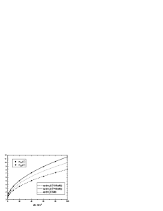
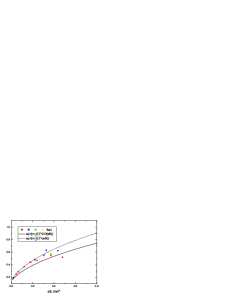
Figure 2: The masses of charged $\pi^{+}$ and $\rho^{+}$ mesons (in GeV) as a function of magnetic field strength at asymptotically large fields (left) and in the region $eB<1$ GeV² in comparison with lattice data of [24] (right).

5 Discussion of results and comparison to lattice data and chiral perturbation theory

As was discussed above, our two examples, $\pi^{0}$ and $\pi^{+}(\pi^{-})$ mesons behave quite differently at strong m.f. and while the first obeys GMOR relations, the charged meson looses all chiral properties at $eB>0.1$ GeV². These facts are in agreement with the results of chiral perturbation theory [25]-[30]. In particular, it was shown in [27, 28] that GMOR relations hold for the $\pi^{0}$ meson, while they are violated for the $\pi^{+}$, and $\pi^{0}$ retains its NG properties in chiral perturbation theory.

However, as shown in [16] and above, both $\langle\bar{q}q\rangle$ and $f^{2}_{\pi}$ are not any more objects of ChPT in strong m.f. and at $eB>m^{2}_{\pi}$ the $q\bar{q}$ degrees of freedom define the values of $\langle\bar{q}q\rangle$ and $f^{2}_{\pi}$.

This in particular is present in the m.f. dependence of $m^{2}_{\pi^{0}}$, which according to ChPT is [27, 28]

$$\frac{m^{2}_{\pi^{0}}(eB)}{m^{2}_{\pi^{0}}(0)}=1-\frac{eB}{16\pi^{2}}\ln 2,$$ (85)

and $e$ is the meson charge in ChPT, while in the $(q\bar{q})$ system two components $(\bar{u}u)$ and $(\bar{d}d)$ enter in an admixture, with $e_{q}=\frac{2}{3}e$ or $\frac{1}{3}e$. We compare the dependence (85) with our result (74) in Fig. 1.

For $\pi^{+}$ meson the ChPT is not applicable for $eB>m^{2}_{\pi}$, while the $q\bar{q}$ structure is clearly seen for $eB>\sigma$, as it is clear from Fig.2, where the curve $m^{2}_{\pi^{+}}(eB)$ deflects from $m^{2}_{\rho^{+}}(eB)$, as discussed in the previous section.

As it is, one can distinguish three regions: 1) $eB\mathrel{\mathchoice{\lower 3.6pt\vbox{\halign{$\mathsurround=0pt\displaystyle\hfil#\hfil$\cr<\crcr\sim\crcr}}}{\lower 3.6pt\vbox{\halign{$\mathsurround=0pt\textstyle\hfil#\hfil$\cr<\crcr\sim\crcr}}}{\lower 3.6pt\vbox{\halign{$\mathsurround=0pt\scriptstyle\hfil#\hfil$\cr<\crcr\sim\crcr}}}{\lower 3.6pt\vbox{\halign{$\mathsurround=0pt\scriptscriptstyle\hfil#\hfil$\cr<\crcr\sim\crcr}}}}m^{2}_{\pi}(0)$, 2) $m^{2}_{\pi}(0)\ll eB\mathrel{\mathchoice{\lower 3.6pt\vbox{\halign{$\mathsurround=0pt\displaystyle\hfil#\hfil$\cr<\crcr\sim\crcr}}}{\lower 3.6pt\vbox{\halign{$\mathsurround=0pt\textstyle\hfil#\hfil$\cr<\crcr\sim\crcr}}}{\lower 3.6pt\vbox{\halign{$\mathsurround=0pt\scriptstyle\hfil#\hfil$\cr<\crcr\sim\crcr}}}{\lower 3.6pt\vbox{\halign{$\mathsurround=0pt\scriptscriptstyle\hfil#\hfil$\cr<\crcr\sim\crcr}}}}\sigma$, 3) $eB\gg\sigma$, where different dominant mechanisms of meson mass formation are present. In the region 1) the ChPT is active for NG mesons, while in the region 2) the $q\bar{q}$ structure is evident and both m.f. effects and strong $q\bar{q}$ interaction (confinement and gluon exchange) are important. Finally in the region 3) one can consider $q$ and $\bar{q}$ in $\pi^{+}$ as independent in the strong m.f. with asymptotic calculated in section 4, while for $\pi^{0}$ the situation is more complicated and the mass is defined by GMOR relations with $\langle q\bar{q}\rangle$ and $f^{2}_{\pi}$ computed in the nonchiral theory.

The authors are grateful to N. O. Agasian, M. A. Andreichikov and B. O. Kerbikov for useful discussions.

Appendix

$$m(\rho^{+}(S_{z}=0),B)=\frac{1}{2}(M_{11}+M_{22})+\sqrt{\left(\frac{M_{11}-M_{22}}{2}\right)^{2}+4a_{12}a_{21}},$$ (A. 1)

$$m(\pi^{+},B)=\frac{1}{2}(M_{11}+M_{22})-\sqrt{\left(\frac{M_{11}-M_{22}}{2}\right)^{2}+4a_{12}a_{21}},$$ (A. 2)

where

$$M_{11}=\bar{M}-\frac{eB}{3\omega_{1}(+-)}+\frac{eB}{6\omega_{1}(+-)}-a_{11}(+-)$$ (A. 3)

$$M_{22}=\bar{M}+\frac{eB}{3\omega_{1}(-+)}-\frac{eB}{6\omega_{1}(-+)}-a_{22}(-+)$$ (A. 4)

and $a_{ik}$ is given in (82), with $c_{ik}$ defined as

$$c_{11}=\frac{8\pi\alpha_{s}}{9\omega_{1}(+-)\omega_{2}(+-)},~{}~{}c_{22}=\frac{8\pi\alpha_{s}}{9\omega_{1}(-+)\omega_{2}(-+)},$$ (A. 5)

and

$$c_{12}c_{21}=\left(\frac{8\pi\alpha_{s}}{9}\right)^{2}\frac{1}{\omega_{1}(+-)\omega_{1}(-+)\omega_{2}(+-)\omega_{2}(-+)}.$$ (A. 6)

The values of $\bar{M}$ can be calculated from (30) or (32), or else for $eB\gg\sigma$ they can be estimated as $\bar{M}\approx\omega_{1}+\omega_{2}=\sqrt{e_{1}B}+\sqrt{e_{2}B}$.

References

[1]
S. L. Glashow and S.Weinberg, Phys. Rev. Lett. 20, 224 (1968);
S. Weinberg, Physica, 96 , A 327 (1979);
M. Gell-Mann and M. Lévy, Nuovo Cimento 16, 53 (1960);
M. Gell-Mann, R.L Oakes, and B. Renner, Phys. Rev. 175, 2195 (1968);
J. Gasser and H. Leutwyler, Phys. Rept. C 87, 77 (1982); Ann. Phys.
(N.Y.) 158, 142 (1984); Nucl. Phys. B 250, 465 (1985);
J. Gasser and H. Leutwyler, Nucl. Phys. B 250, 465 (1985);
C. W. Bernard and M. F. L. Golterman, Phys. Rev. D 46, 853 (1992);
S. R. Sharpe, Phys. Rev. D 46, 3146 (1992).
[2] Yu. A. Simonov,
Phys. Rev. D 65, 094018 (2002); hep-ph/0201170.
[4]Yu. A. Simonov, Phys. Atom. Nucl. 67, 1027 (2004);
hep-ph/0305281.
[5] S. M. Fedorov and
Yu. A. Simonov, JETP Lett. 78, 57 (2003); hep-ph/0306216.
[6]
A. Yu. Dubin, A. B. Kaidalov, and Yu. A. Simonov, Phys. Atom. Nucl. 56,
1745 (1993); Phys. Lett. B 323, 41 (1994);
Yu. S. Kalashnikova, A. V. Nefediev, and Yu. A. Simonov, Phys. Rev. D 64,
014037 (2001).
[8] D.E.Kharzeev, K.Landsteiner, A.Schmitt, H.-U.Yee, “Strongly interacting matter in
magnetic fields”,Lect Notes in Phys. (Springer); arXiv:1211.6245.
[9]
J.M.Lattimer and M.Prakash, Phys. Rept. 442, 109 (2007).
[10] D. Grasso and H. Rubinstein, Phys. Rept. 348, 163 (2001).
[11]
D.E.Kharzeev, L.D.McLerran and H.J.Warringa, Nucl. Phys. A803, 227
(2008);
V.Skokov, A.Illarionov and V.Toneev, Int. J. Mod. Phys. A24,
5925 (2009).
[12]
B.M.Karnakov and V.S.Popov, J. Exp. Theor. Phys. 97, 890
(2003); ZhETF 141, 5 (2012).
[13] M. A. Andreichikov, B. O. Kerbikov and Yu.A.Simonov, arXiv:
1210.0227.
[14] M. A. Andreichikov, V. D. Orlovsky and Yu.A.Simonov, arXiv:
1211.6568; M. A. Andreichikov, B. O. Kerbikov, V. D. Orlovsky and
Yu. A. Simonov, arXiv:1304.2533; Phys. Rev. D.
[15]
A. M. Badalian and Yu. A. Simonov, (Phys. Rev. D. 87, 074012 (2013) ), arXiv:1211.4349.
[16] Yu. A. Simonov, arXiv:
1212.3118.
[17] M.D’Elia, S.Mukherjiee and F.Sanfilippo, Phys. Rev. D 82,
051501 (2010); arXiv:1005.5365;
M.D’Elia and F.Negro, Phys. Rev. D 83, 114028 (2011); arXiv:1103.2080;
M.D’Elia, arXiv:1209.0374.
[18] P.Buividovich, M.Chernodub, E.Luschevskaya and M.Polikarpov,
Phys. Lett. B 682, 484 (1010); arXiv:0812.1740;
V.Braguta, P.Buividovich, T.Kalaydzhyan, S.Kusnetsov and
M.Polikarpov, PoS Lattice 2010, 190 (2010); arXiv:1011.3795.
[19] E.-M.Ilgenfritz et al., arXiv:1203.3360.
[20] G.S.Bali, F.Bruckmann, G.Enrödi, Z.Fodor, S.D.Katz and
A.Schäfer, Phys. Rev. D 86,071502 (2012); arXiv:1206.4205.
[21] Yu.A.Simonov, arXiv:1303.4952.
[22] Y.Hidaka and A.Yamamoto, arXiv: 1209.0007 [hep-lat].
[23] Yu. A. Simonov, arXiv: 1304.0365.
[24] G.S.Bali, F.Bruckmann, G.Endrodi et al., JHEP 1202, 044 (2012).
[25] S. Weinberg, Physica A 96, 327 (1979).
[26] J. Gasser and H. Leutwyler, Ann. Phys. 158, 142 (1984);
Nucl. Phys. B250, 465 (1985).
[27] I. A. Shushpanov and A. V. Smilga, Phys. Lett. B402, 351 (1997).
[28] N. O. Agasian and I. A. Shushpanov, JETP Lett. 70, 717 (1999);
Phys. Lett. B472, 143 (2000); JHEP 0110, 006 (2001).
[29] N. O. Agasian, Phys. Lett. B488, 39 (2000); Phys. Atom. Nucl. 64, 554 (2001).
[30] J. O. Andersen, JHEP, 1210, 005 (2012); Phys. Rev. D86, 025020 (2012).