Quantum-critical pairing in electron-doped cuprates

Abstract

We revisit the problem of spin-mediated superconducting pairing at the antiferromagnetic quantum-critical point with the ordering momentum $(\pi,\pi)=2{\bf k}_{F}$. The problem has been previously considered by one of the authors [P. Krotkov and A. V. Chubukov, Phys. Rev. Lett. 96, 107002 (2006); Phys. Rev. B 74, 014509 (2006)]. However, it was later pointed out [D. Bergeron et al., Phys. Rev. B 86, 155123 (2012)] that that analysis neglected umklapp processes for the spin polarization operator. We incorporate umklapp terms and re-evaluate the normal state self-energy and the critical temperature of the pairing instability. We show that the self-energy has a Fermi-liquid form and obtain the renormalization of the quasiparticle residue $Z$, the Fermi velocity, and the curvature of the Fermi surface. We argue that the pairing is a BCS-type problem, but go one step beyond the BCS theory and calculate the critical temperature $T_{c}$ with the prefactor. We apply the results to electron-doped cuprates near optimal doping and obtain $T_{c}\geq 10\rm K$, which matches the experimental results quite well.

I Introduction

Superconductivity near a quantum-critical point (QCP) in a metal is one of the most studied and debated topics in the physics of strongly correlated electron systems subir_book ; piers_andy ; acs ; tremblay . When a metal is brought, by doping, external field, or pressure, to a near vicinity of a phase transition into a state with either spin or charge density-wave order, corresponding collective bosonic excitations become soft and fermion-fermion interaction, mediated by collective bosons, gets enhanced. Quite often, this interaction turns out to be attractive in one or the other pairing channel, and gives rise to enhanced superconducting $T_{c}$ near a QCP. Examples of the pairing mediated by soft bosonic fluctuations include the pairing in double-layer composite fermion metals nick , pairing due to singular momentum-dependent interaction extra , color superconductivity of quarks mediated by gluon exchange color , pairing by singular gauge fluctuations gauge ; aim_el ; ms_1 , pairing by near-critical ferromagnetic and antiferromagnetic spin fluctuations fm_qcp ; afm_qcp ; acf ; lonz-pines ; ms_2 ; efetov ; am_qcp ; moon_sa , and phonon-mediated pairing at vanishing Debye frequency phonons .

The pairing at a QCP in dimensions $D\leq 3$ is generally a non-trivial problem because near a QCP fermions do not display a conventional Fermi-liquid (FL) behavior down to the smallest frequencies, at least in some (hot) regions on the Fermi Surface (FS). To obtain the pairing instability in this situation one has to go beyond the leading logarithmical approximation as the summation of the leading logarithms does not lead to an instability acf ; wang , except for a special case of a color superconductivity color .

Pairing near the ${\bf Q}=(\pi,\pi)$ antiferromagnetic QCP attracted most of the attention in recent years, particularly in $D=2$, because of its relation to $d$-wave superconductivity in the cuprates. acs ; lonz-pines ; ms_2 ; efetov ; scal_1 ; scal ; moria ; manske ; ramisak ; FLEX ; X ; mar_fit . The FS in hole-doped cuprates around optimal doping is an open electron FS (closed hole FS) which contains four pairs of hot spots (points for which ${\bf k}_{F}$ and ${\bf k}_{F}+{\bf Q}$ are both on the FS). The hot spots are located near $(0,\pi)$ and other symmetry-related points. At each hot spot, fermionic self-energy at a QCP has a non-FL form $\Sigma(\omega)\propto\omega^{a}$ with $a\approx 1/2$, down to the lowest frequencies millis_1/2 ; acs ; ms_2 ; senthil . The pairing of these hot fermions, the relative role of quasiparticles with non-FL and FL forms of the self-energy, and the interplay between the pairing and the bond-order instabilities near a QCP are intriguing phenomena which are not fully understood yet, but for which a strong progress has been made theoretically in the last few years ms_2 ; efetov ; wang .

The present work is devoted to the analysis of superconductivity at the antiferromagnetic QCP, but in the special case when ${\bf Q}$ coincides with $2{\bf k}_{F}$ along the diagonals in the Brillouin zone (see FIG. 2) aim_el . In this situation, there are only two pairs of hot spots, located along the two diagonals of the Brillouin zone, and for each pair Fermi velocities at ${\bf k}_{F}$ and ${\bf k}_{F}+{\bf Q}$ are strictly antiparallel. This case is applicable to electron-doped cuprates ${\rm Nd}_{2-x}{\rm Ce}_{x}{\rm Cu}_{3}{\rm O}_{7}$ and ${\rm Pr}_{2-x}{\rm Ce}_{x}{\rm Cu}_{3}{\rm O}_{7}$ el_rmp . The FS of these materials near the onset of spin density wave (SDW) order has four pairs of hot spots located close enough to zone diagonals. This makes our model a good starting point. As $T_{c}$ only increases as hot spots move apart (see below), our result places the lower boundary on $T_{c}$ in these materials.

The phase diagram of electron doped cuprates is somewhat better understood than that of hole-doped materials in the sense that the pseudogap physics of these materials is most likely due to magnetic precursors  tremblay_1 ; el_rmp ; zimmers ; koitzsch03 ; Aiff03 ; greven . This in turn implies that magnetic fluctuations are strong and well may be relevant to superconductivity. An earlier RPA study has found onufr that the electron doping, at which magnetic order emerges, is close to the one at which hot spots merge along zone diagonals. At larger electron doping, there are no hot spots and no magnetism. At smaller dopings, magnetic order emerges and, simultaneously, each pair of diagonal hot spots splits into two pairs which move away from diagonals in two different directions.

The quantum-critical pairing near a $2{\bf k}_{F}$ QCP has been earlier considered by one of us in Refs. krotkov ; dan . It was found that there is a sizable attraction in the $d_{x^{2}-y^{2}}$ channel, despite that at $2{\bf k}_{F}$ QCP the strongest interaction connects the points where $d_{x^{2}-y^{2}}$ gap vanishes. This result stands. However, the value of $T_{c}$ has to be reconsidered because the analysis in krotkov ; dan used for the normal state self-energy at the hot spots the non-FL form $\Sigma(\omega)=\omega^{3/4}$, which was obtained in krotkov and in earlier work aim_el by neglecting umklapp processes. Recent study subir_el has found that umklapp processes severely reduce the self-energy, such that quasiparticles remain coherent even at a QCP. The imaginary part of the self-energy at the QCP scales as $\omega^{3/2}\log\omega$, i.e., the Fermi liquid is non-canonical in the notations of  maslov , but, still, ${\rm Im}\Sigma\ll\omega$ at small frequency, and the Fermi liquid criteria of long-lived quasiparticles near the FS remains valid. Whether the $\omega^{3/2}$ self-energy is responsible for the observed $T^{1.6}$ behavior of resistivity in overdoped La_2-xCe_xCuO₄ (Ref. [rick, ]) remains to be seen.

In this paper, we reconsider the problem of the pairing at the $2{\bf k}_{F}$ QCP using the correct form of the self-energy. We show that the pairing is a FL phenomenon, i.e., it is fully determined by the coherent component of the quasiparticle Green’s function and depends on the quasiparticle $Z$ factor and the effective mass. Moreover, when spin-fermion coupling is small compared to the Fermi energy, the pairing can be analyzed within the weak coupling, BCS-type analysis. Our goal is to go one step beyond the BCS theory and compute $T_{c}$ exactly, with the numerical prefactor.

The calculation we present here is similar in spirit to the one done in early days of BCS superconductivity for a model of fermions with a constant attractive interaction gorkov-melik , but is more involved, as in our case the pairing interaction contains the propagator of low-energy collective bosons which strongly depends on the transferred momentum and the transferred frequency. We show that these two dependencies make calculations somewhat tricky, but still doable.

We consider the low-energy model of fermions located near Brillouin zone diagonals and assume that fermions interact by exchanging near-critical soft collective fluctuations in the spin channel (the spin-fermion model). The model contains two parameters: the overall energy scale ${\bar{g}}$, which is the effective fermion-fermion interaction mediated by spin fluctuations, and the dimensionless coupling $\lambda$, which determines mass renormalization and the renormalization of the quasiparticle $Z$ factor acs ; ms_2 . In our case, the coupling $\lambda$ is one-third power of the ratio of ${\bar{g}}$ and the effective Fermi energy of quasiparticles near Brillouin zone diagonal:

$$\lambda=\left(\frac{{\bar{g}}}{4\pi E_{F}}\right)^{1/3},$$ (1)

We approximate the fermionic dispersion near Brillouin zone diagonals by $\epsilon_{k}=v_{F}(k_{x}+\kappa k^{2}_{y}/2)$, where $k_{x}$ and $k_{y}$ are the directions along and transverse to zone diagonals, measured relative to a hot spot, $v_{F}$ is the Fermi velocity along zone diagonal and $\kappa$ is the curvature of the FS. In terms of these parameters $E_{F}=v_{F}/(2\kappa)$.

In the normal state we found that the quasiparticle residue $Z$, the Fermi velocity $v_{F}$, and the curvature $\kappa$ differ from free-fermion values by corrections of order $\lambda$:

$$Z=1-0.7\lambda,~{}~{}v^{*}_{F}=v_{F}(1+0.05\lambda),~{}~{}\kappa^{*}=\kappa(1-1.45\lambda),$$ (2)

Observe that the renormalizations of $Z$ and $v^{*}_{F}$ do not satisfy $Zv_{F}/v^{*}_{F}=1$, which holds in Eliashberg-type theories (ET’s) of electron-phonon phonons and electron-electon acs ; acf interactions. A similar result was obtained in the calculation of self-energy in the AFM state das2 . ramisek The reason for the discrepancy with ET’s is quite fundamental: in ET’s the self-energy $\Sigma({\bf k},\omega_{m})\approx i\lambda\omega_{m}$ depends only on frequency and comes from intermediate fermions with energies comparable to $\omega_{m}$, other corrections are relatively small in Eliashberg parameter ($(\omega_{D}/E_{F})^{1/2}$ for electron-phonon interaction). In our case, Eliashberg parameter is of order one, and there are two contributions to $\Sigma({\bf k},\omega_{m})$ of comparable strength. One comes from intermediate fermions with energies comparable to $\omega_{m}$ and scales as $\omega_{m}$, i.e., depends only on frequency. The other comes from intermediate fermions with energies much larger than $\omega_{m}$, and scales as $i\omega_{m}+v_{F}(k-k_{F})$. Because the two contributions are of the same order, $\partial\Sigma/\partial(i\omega_{m})$ and $(1/v_{F})\partial\Sigma/\partial k$ are comparable. As a result, the renormalizations of $Z$ and of Fermi velocity are comparable in strength (both are of order $\lambda$), but the prefactors are different.

We used normal state results as an input for the pairing problem and computed superconducting $T_{c}$ at the QCP. We found

$$T_{c}=0.0013~{}\frac{\bar{g}}{\lambda}~{}e^{-\frac{C}{\lambda}},~{}~{}C=0.6874$$ (3)

The exponential dependence on $\lambda$ and the overall factor ${\bar{g}}/\lambda$ can be obtained within logarithmical BCS-type treatment. However, to obtain the overall numerical factor in (3), we had to go beyond the logarithmical approximation and use the fact that theramisek boson-mediated interaction is dynamical and decays at large frequencies. This part of our analysis is similar to the calculation of $T_{c}$ in ETs phonons ; acf . However, as we said, the similarity is only partial because the renormalized Green’s function in our case is different from the one in ET. In another distinction from ET, in our case we need to include into consideration non-ladder diagrams which account for Kohn-Luttinger-type renormalization of the pairing interaction kl . These diagrams do not affect the exponent but contribute $O(1)$ to the numerical prefactor in $T_{c}$. In ET theories, the contribution from Kohn-Luttinger renormalizations is small in Eliashberg parameter.

We plot $T_{c}/{\bar{g}}$ as a function of $\lambda$ in FIG. 1. We see that $T_{c}$ increases with $\lambda$ at small $\lambda$, passes through a broad maximum at $\lambda\sim 0.5$ and slowly decreases at larger $\lambda$. The actual value of $\lambda$ can be extracted from the data. The energy ${\bar{g}}$ can be deduced from optical measurements in the magnetically ordered Mott-Heisenberg state at half-filling optics_el where ${\bar{g}}$ coincides with the optical gap. The data yield ${\bar{g}}\sim 1.6-1.7\rm eV$, which is essentially the same as in hole-doped cuprates (this scale is close to the charge-transfer energy $U$ in the effective Hubbard model). The Fermi velocity $v_{F}$ and the curvature $\kappa$ can be extracted from the ARPES measurements of optimally doped ${\rm Nd}_{2-x}{\rm Ce}_{x}{\rm Cu}_{3}{\rm O}_{7}$ exp_el . The fit yields $v_{F}=0.87\rm eV$, $\kappa=0.31$, and the effective Fermi energy $E_{F}=v_{F}/(2\kappa)\sim 1.4\rm eV$. Substituting into (2) we obtain $\lambda\sim 0.46$. For such $\lambda$, $Z\approx 0.7$, i.e., weak coupling approximation is reasonably well justified. Using $\lambda=0.46$ and ${\bar{g}}=1.7\rm eV$, we obtained $T_{c}=0.0006{\bar{g}}\sim 12\rm K$. This value is actually the lower theoretical boundary on $T_{c}$ by two reasons. One is theoretical – we found that $T_{c}$ get enhanced if we keep the fermionic bandwidth (the upper limit of the low-energy theory) finite. The second is practical – in optimally doped ${\rm Nd}_{2-x}{\rm Ce}_{x}{\rm Cu}_{3}{\rm O}_{4}$ and ${\rm Pr}_{2-x}{\rm Ce}_{x}{\rm Cu}_{3}{\rm O}_{4}$ hot spots are located close to, but still at some distance from zone diagonals el_rmp . When they are far apart, $T_{c}$ is much higher wang ; norman_1 , and it is natural to expect that $T_{c}$ gets higher when hot spots split.ramisek Another feature of real materials, which may affect $T_{c}$ a bit, is the observation greven that SDW antiferromagnetism and superconductivity in ${\rm Nd}_{2-x}{\rm Ce}_{x}{\rm Cu}_{3}{\rm O}_{4+\delta}$ may be actually separated by weak first-order transition rather than co-exist dagan04 , in which case the magnetic correlation length remains large but finite at optimal doping. Still, the value which we found theoretically is in quite reasonable agreement with the experimental $T_{c}\sim 10-25\rm K$ in ${\rm Nd}_{2-x}{\rm Ce}_{x}{\rm Cu}_{3}{\rm O}_{4}$ and in ${\rm Pr}_{2-x}{\rm Ce}_{x}{\rm Cu}_{3}{\rm O}_{4}$ (Refs. takagi ; TC2 ). Also, our $\lambda=0.46$ is close to the position of the broad maximum of $T_{c}(\lambda)$ in FIG. 1, hence $T_{c}$ only slightly increases or decreases if the actual $\lambda$ differs somewhat from our estimate.

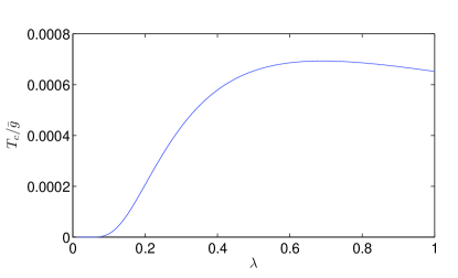
Figure 1: The critical temperature $T_{c}/\bar{g}$ as a function of the coupling $\lambda$.

The paper is organized as follows. In the next section we introduce the spin-fermion model as the minimal model to describe interacting fermions near the $2{\bf k}_{F}$ spin-density-wave instability. In Sec. III we present one-loop normal state calculations, which include umklapp scattering. We obtain the spin polarization operator, which accounts for the dynamics of collective excitations, and use it to obtain fermionic self-energy to first order in $\lambda$. In Sec. IV we solve for $T_{c}$ in one-loop (ladder) approximation. We show that $T_{c}$ is exponentially small in $\lambda$ and find the prefactor to one-loop order. In Sec. V we analyze two-loop corrections to $T_{c}$ and show that they change the numerical prefactor for $T_{c}$ by a finite amount. We argue that higher-loop corrections are irrelevant as they only change $T_{c}$ by a factor $1+O(\lambda)$. Combining one-loop and two-loop results, we obtain the full expression for $T_{c}$ at weak coupling, Eq. (63). We also discuss in Sec. V the effect on $T_{c}$ from lowering the upper energy cutoff $\Lambda$ of the theory. When $\Lambda$ is of order bandwidth, $W$, $T_{c}$ is essentially independent on $\Lambda$ as long as $T_{c}\ll W$. However, if, by some reasons, $\Lambda$ is smaller that $W$, $T_{c}$ gets larger, and its increase becomes substantial when $\Lambda<{\bar{g}}^{1/3}W^{2/3}$. We compare our results with the experiments in Sec. VI and summarize our results in Sec. VII.

II The model

We consider fermions on a square lattice at a density larger than one electron per cite (electron doping) and use tight-binding form of electron dispersion with hopping to first and second neighbors. We choose doping at which free-fermion FS touches the magnetic Brillouin zone along the diagonals, as shown in FIG. 2. We assume, following earlier works onufr , that at around this doping the system develops a spin-density-wave (SDW) order with momentum ${\bf Q}=(\pi,\pi)$. For convenience, throughout the paper we will use a rotated reference frame with $(k_{x},k_{y})$ shown in FIG. 2. In this frame, the SDW ordering momentum is $(0,\sqrt{2}\pi)$ or $(\sqrt{2}\pi,0)$.

We analyze the physics near the ${\bf Q}=2{\bf k}_{F}$ antiferromagnetic QCP within the semi-phenomenological spin-fermion model acs ; acf ; ms_2 ; efetov ; aim_el ; krotkov ; subir_el . The model assumes that antiferromagnetic correlations develop already at high energies, comparable to bandwidth, and mediate interactions between low-energy fermions. In the context of superconductivity, spin-mediated interaction then plays the same role of a pairing glue as phonons do in conventional superconductors. The static part of the spin-fluctuation propagator comes from high-energies and should be treated as an input for low-energy theory. However, the dynamical part of the propagator should be self-consistently obtained within the model as it comes entirely from low-energy fermions.

The Lagrangian of the model is given by acs ; ms_2 ; efetov

$${\mathcal{S}}= -\int_{k}^{\Lambda}G_{0}^{-1}\left(k\right)\psi_{k,\alpha}^{\dagger}\psi_{k,\alpha}+\frac{1}{2}\int_{q}^{\Lambda}\chi_{0}^{-1}\left(q\right)\ {\bf{S}}_{q}\cdot{\bf{S}}_{-q}$$

$$+g\int_{k,q}^{\Lambda}\psi_{k+q,\alpha}^{\dagger}\sigma_{\alpha\beta}\psi_{k,\beta}\cdot{\bf{S}}_{-q}.\$$ (4)

where $\int_{k}^{\Lambda}$ stands for the integral over $d-$dimensional ${\bf{k}}$ (up to some upper cutoff $\Lambda$) and the sum runs over fermionic and bosonic Matsubara frequencies. The $G_{0}\left(k\right)=G_{0}({\bf k},\omega_{m})=1/(i\omega_{m}-\epsilon_{\bf k})$ is the bare fermion propagator and $\chi_{0}\left({\bf q}+{\bf Q}\right)=\chi_{0}/({\bf q}^{2}+\xi^{-2})$ is the static propagator of collective bosons, in which $\xi^{-1}$ measures the distance to the QCP, and ${\bf q}$ is measured with respect to ${\bf Q}$. At the QCP, $\xi^{-1}=0$. The fermion-boson coupling $g$ and $\chi_{0}$ appear in theory only in combination ${\bar{g}}=g^{2}\chi_{0}$, which has the dimension of energy.

The interaction between fermions and collective spin bosons gives rise to fermionic self-energy $\Sigma({\bf k},\omega_{m})$, which modifies fermionic propagator to $G^{-1}({\bf k},\omega_{m})=G^{-1}_{0}({\bf k},\omega_{m})+\Sigma({\bf k},\omega_{m})$, and bosonic self-energy which modifies bosonic propagator to $\chi^{-1}\left({\bf q}+{\bf Q},\Omega_{m})\right)=\left({\bf q}^{2}+\xi^{-2}+\Pi\left({\bf q}+{\bf Q},\Omega_{m}\right)\right)/\chi_{0}$. We focus on the hot regions on the FS, which are most relevant to the pairing when ${\bar{g}}$ is smaller than the cutoff $\Lambda$. In our case, there are four hot regions around Brillouin zone diagonals, which we labeled $1$ to $4$ in FIG. 2. The physics in one hot region is determined by the interaction with another hot region, separated by ${\bf Q}$. This creates two “pairs” – (1, 4), and (2, 3). However, the pairs cannot be fully separated because ${\bf Q}$ and $-{\bf Q}$ differ by inverse lattice vector, hence umklapp processes arramiseke allowed subir_el . As a result, the interaction between fermions in regions $1$ and $4$ is mediated by $\chi({\bf q}+{\bf Q},\Omega_{m})$ whose polarization operator $\Pi({\bf q}+{\bf Q},\Omega_{m})$ has contribution from fermions in the same regions 1 and 4, but also from fermions in the regions 2 and 3.

We define fermion momenta relative to their corresponding hot spots. The dispersion of a fermion is linear in transverse momentum (the one along the Brillouin zone diagonal) and quadratic in the momentum transverse to the diagonal. Specifically, the dispersion relation in region 1 is

$$\epsilon_{k}=-v_{F}\left(k_{x}+\kappa\frac{k_{y}^{2}}{2}\right),$$ (5)

where $\kappa$ is the curvature of the FS.

Figure 2: Fermi surface at a particular electron doping when the Fermi surface touches the magnetic Brillouin zone along the zone diagonals. The four diagonal Fermi surface points (hot spots) are labeled by numbers. We assume that this doping is close to the one at which antiferromagnetic instability emerges at momentum ${\bf Q}=(\pi,\pi)$.

III Normal State Analysis

The spin polarization operator $\Pi({\bf q}+{\bf Q},\Omega_{m})$ is the dynamical part of the particle-hole bubble with external momentum near ${\bf Q}$. The dressed dynamical spin fluctuations give rise to fermionic self-energy $\Sigma({\bf k},\omega_{m})$, which in turn affects the form of $\Pi({\bf q}+{\bf Q},\Omega_{m})$. This mutual dependence generally implies that $\Sigma({\bf k},\omega_{m})$ and $\Pi({\bf q}+{\bf Q},\Omega_{m})$ form a set of two coupled equations. When hot spots are far from zone diagonals and Fermi velocities at ${\bf k}_{F}$ and ${\bf k}_{F}+{\bf Q}$ are not antiparallel (like in hole-doped cuprates), the two equations decouple because the bosonic polarization operator has the Landau damping form $\Pi({\bf q}+{\bf Q},\Omega_{m})=\gamma|\Omega_{m}|$, and the prefactor $\gamma$ does not depend on fermionic self-energy as long as the latter predominantly depends on frequency. Evaluating fermionic $\Sigma$ with the Landau overdamped $\chi({\bf q}+{\bf Q},\Omega_{m})$ one can in turn verify acs ; ms_2 that $\Sigma$ predominantly depends on frequency near a QCP, i.e., equations for $\Sigma({\bf k},\omega_{m})\approx\Sigma(\omega_{m})$ and $\Pi({\bf q}+{\bf Q},\Omega_{m})$ do indeed decouple. This decoupling allows one to compute the Landau damping using free-fermion propagator, even when $\Sigma(\omega_{m})$ is not small, and use the dynamical $\chi({\bf q}+{\bf Q},\Omega)$ with Landau damping term in the calculations of the fermionic self-energy comm_a In our case, the dynamical part of $\chi$ is not Landau damping because Fermi velocities at ${\bf k}_{F}$ and ${\bf k}_{F}+{\bf Q}$ are strictly antiparallel, and $\Pi({\bf q}+{\bf Q},\Omega_{m})$ does depend on fermionic self-energy dan . This generally requires full self-consistent analysis of the coupled set of non-linear equations for $\Sigma({\bf k},\omega_{m})$ and $\Pi({\bf q}+{\bf Q},\Omega_{m})$. Fortunately, in our case the system preserves a FL behavior even at the QCP, and for ${\bar{g}}<W$, which we assume to hold, calculations can be done perturbatively rather than self-consistently. Below we will obtain lowest-order (one-loop) expressions for the polarization bubble and fermionic self-energy and use them to compute $T_{c}$ in the ladder approximation. We then discuss how these expressions are affected by two-loop diagrams.

III.1 One-loop bosonic and fermionic self-energies

The one-loop Feynman diagram for the polarization operator is shown in FIG. 3.

Figure 3: The one-loop polarization bubble. Labels $i$ and $j$ denotes fermions at different hot spots. The full expression is the sum of direct and umklapp processes, $(1,4),(4,1)$, $(2,3),(3,2)$.

The polarization operator contains contributions from direct and umklapp scattering between hot spots separated by either ${\bf Q}$ or $-{\bf Q}$ (the combinations of $(i,j)$ of internal fermions can be $(1,4),(4,1),(2,3),$ and $(3,2)$. For external momenta near ${\bf Q}=(\pi,\pi)$, the processes $(1,4)$ and $(4,1)$ are direct and $(2,3)$ and $(3,2)$ are umklapp. Only direct processes have been considered in Ref. [aim_el, ; krotkov, ], but, as was pointed out in subir_el , all four processes should be included into $\Pi$. The authors of Ref. [subir_el, ] obtained

$$\Pi({\bf q}+{\bf Q},\Omega)= \Pi^{(0)}(q_{x},q_{y},\Omega)+\Pi^{(0)}(-q_{x},q_{y},\Omega)$$

$$+ \Pi^{(0)}(q_{y},q_{x},\Omega)+\Pi^{(0)}(-q_{y},q_{x},\Omega),$$ (6)

where aim_el ; krotkov

$$\Pi^{(0)}(q_{x},q_{y},\Omega)=\frac{{\bar{g}}}{\pi\sqrt{2v_{F}^{3}\kappa}}\sqrt{\sqrt{\Omega^{2}+E_{q}^{2}}+E_{q}},$$ (7)

and

$$E_{q}=v_{F}\left(q_{x}-\kappa\frac{q_{y}^{2}}{4}\right).$$ (8)

The full dynamical spin susceptibility is

$$\chi({\bf q}+{\bf Q},\Omega)=\frac{\chi_{0}}{{\bf q}^{2}+\Pi({\bf q}+{\bf Q},\Omega)}.$$ (9)

We now use $\chi({\bf q},\Omega)$ from (9) and calculate one-loop self-energy of an electron. We will see that relevant ${\bf q}^{2}$ and $\Pi({\bf q}+{\bf Q},\Omega)$ are of the same order, i.e., the spin-plolarization operator evaluated at one-loop order is not a small perturbation of the bare static $\chi_{0}({\bf q}+{\bf Q})$. Higher-loop terms in $\Pi({\bf q}+{\bf Q},\Omega)$ are, however, small in $\lambda$ and can be treated perturbatively.

The one loop self-energy is presented diagrammatically in FIG. 4.

Figure 4: One-loop electron self-energy.

Specifically, close to the hot spot, labeled by 1, the analytical expression is,

$$\Sigma({\bf k},\omega_{m})=$$

$$-\frac{3\bar{g}}{8\pi^{3}}\int\frac{d{\bf q}~{}d\Omega_{m}}{i(\omega_{m}+\Omega_{m})-\epsilon_{{\bf k}+{\bf q}+{\bf Q}}}\frac{1}{{\bf q}^{2}+\Pi({\bf q}+{\bf Q},\Omega_{m})},$$ (10)

where, as before, the momenta ${\bf k}$ and ${\bf k+q}$ are taken close to hot spots 1 at $(-k_{F},0)$, and 4 at $(k_{F},0)$, and the dispersion $\epsilon_{{\bf k}+{\bf Q}}$ is

$$\epsilon_{{\bf k}+{\bf Q}}=-v_{F}\left(-k_{x}+\kappa\frac{k_{y}^{2}}{2}\right)=\epsilon_{-{\bf k}}.$$ (11)

The coefficient 3 comes from summation over the $x,y$, and $z$ components of the spin susceptibility.

For definiteness, we consider the self-energy right at the QCP, when $\xi^{-1}=0$. We assume and then verify that FL behavior is preserved at the QCP, i.e. at small $\omega_{m}$, $\Sigma(0,\omega_{m})=i\lambda\omega_{m}$ and $\Sigma(k_{x},0)\propto v_{F}k_{x}$, $\Sigma(k_{y},0)\propto k^{2}_{y}$, We will need both frequency and momentum-dependent components of the self-energy for the calculation of $T_{c}$.

To compute $\Sigma$, it is convenient to subtract from $\Sigma({\bf k},\omega_{m})$ its expression at ${\bf k}=0$ and $\omega_{m}=0$ as the latter vanishes by symmetry for our approximate form of the dispersion $\epsilon_{k}$. This subtraction can actually be done even if one does not approximate $\epsilon_{k}$, as, in the most general case, $\Sigma(0,0)$ accounts only for the renormalization of the chemical potential by fermions with energies above $\Lambda$, which we have to neglect anyway to avoid double counting as such renormalization is already included into $\epsilon_{k}$. After the subtraction, the self-energy becomes

$$\Sigma({\bf k},\omega_{m})= \frac{3\bar{g}}{8\pi^{3}}\int d{\bf q}~{}d\Omega_{m}\frac{1}{{\bf q}^{2}+\Pi({\bf q}+{\bf Q},\Omega_{m})}$$

$$\times \frac{i\omega_{m}-\left[\epsilon_{-(q+k)}-\epsilon_{-q}\right]}{(i\Omega_{m}-\epsilon_{-q})\left[i(\omega_{m}+\Omega_{m})-\epsilon_{-(q+k)}\right]},$$ (12)

It is tempting to set $\omega_{m}$ and $k$ to zero in the denominator of (12) but this would lead to an incorrect result as the integrand in (12) contains two close poles, and the contribution from the region between the poles is generally of order one acs . To obtain the correct self-energy one has to explicitly integrate over internal frequency and momenta without setting $\omega_{m}$ and $k$ to zero. The order of integration doesn’t matter because the integral is convergent in the ultra-violet limit. We choose to integrate over $q_{x}$ first as this will allow us to make a comparison with hole-doped cuprates.

The integral in (12) above can be simplified if we introduce the dimensionless small parameter

$$\lambda\equiv\left(\frac{{\bar{g}\kappa}}{2\pi v_{F}}\right)^{1/3}=\left(\frac{{\bar{g}}}{4\pi E_{F}}\right)^{1/3}$$ (13)

and rescale

$$\Sigma\rightarrow\frac{{\bar{g}}{\tilde{\Sigma}}}{\pi\lambda},~{}~{}q\rightarrow\frac{\bar{g}\tilde{q}}{v_{F}\pi\lambda},~{}~{}k\rightarrow\frac{\bar{g}\tilde{k}}{v_{F}\pi\lambda}$$

$$\Omega_{m}\rightarrow\frac{\bar{g}{\tilde{\Omega}}_{m}}{\pi\lambda},~{}~{}\omega_{m}\rightarrow\frac{\bar{g}{\tilde{\omega}}_{m}}{\pi\lambda},$$ (14)

In the new variables,

$$~{}~{}~{}~{}~{}~{}~{}~{}~{}~{}~{}~{}\epsilon_{q,k}=\frac{\bar{g}}{\pi\lambda}{\tilde{\epsilon}}_{{\tilde{q}}.{\tilde{k}}},~{}~{}~{}~{}{\bf q}^{2}=\left(\frac{\bar{g}}{\pi v_{F}\lambda}\right)^{2}{\tilde{\bf q}}^{2},$$

$$\Pi\left({\bf q}+{\bf Q},\Omega_{m}\right)=\left(\frac{\bar{g}}{\pi v_{F}\lambda}\right)^{2} \left[\tilde{\Pi}^{(0)}\left({\tilde{q}_{x}},{\tilde{q}}_{y},{\tilde{\Omega}}_{m}\right)+\tilde{\Pi}^{(0)}\left(-{\tilde{q}_{x}},{\tilde{q}}_{y},{\tilde{\Omega}}_{m}\right)+\tilde{\Pi}^{(0)}\left({\tilde{q}_{y}},{\tilde{q}}_{x},{\tilde{\Omega}}_{m}\right)+\tilde{\Pi}^{(0)}\left(-{\tilde{q}_{y}},{\tilde{q}}_{x},{\tilde{\Omega}}_{m}\right)\right]$$ (15)

where

$${\tilde{\epsilon}}_{{\tilde{q}}}= -{\tilde{q}}_{x}-\lambda^{2}{\tilde{q}}^{2}_{y},$$

$${\tilde{\Pi}}^{(0)}\left({\tilde{q}_{x}},{\tilde{q}}_{y},{\tilde{\Omega}}_{m}\right)= \frac{1}{2}\sqrt{\sqrt{{\tilde{\Omega}}^{2}_{m}+{\tilde{E}}^{2}_{\tilde{q}}}+{\tilde{E}}_{\tilde{q}}},$$

$${\tilde{E}}_{\tilde{q}}= {\tilde{q}}_{x}-\frac{\lambda^{2}{\tilde{q}}^{2}_{y}}{2}.$$ (16)

Substituting these expressions into (12) we find that the rescaled self-energy is the function of a single parameter $\lambda$:

$${\tilde{\Sigma}}({\bf{\tilde{k}}},\omega_{m})=\frac{3\lambda}{8\pi^{2}}\int\frac{d{\tilde{q}}_{x}~{}d{\tilde{q}}_{y}~{}d{\tilde{\Omega}}_{m}}{{\bf\tilde{q}}^{2}+\sum_{a=\pm 1}{\tilde{\Pi}}_{a}^{(0)}({\bf\tilde{q}},{\tilde{\Omega}}_{m})}\times$$

$$\frac{i{\tilde{\omega}}_{m}-{\tilde{k}}_{x}+\lambda^{2}({\tilde{k}}^{2}_{y}+2{\tilde{k}}_{y}{\tilde{q}}_{y})}{(i{\tilde{\Omega}}_{m}-{\tilde{q}}_{x})\left[i({\tilde{\Omega}}_{m}+{\tilde{\omega}}_{m})-{\tilde{q}}_{x}-{\tilde{k}}_{x}+\lambda^{2}({\tilde{k}}^{2}_{y}+2{\tilde{k}}_{y}{\tilde{q}}_{y})\right]},$$ (17)

where ${\tilde{\Pi}}_{a}^{(0)}({\bf{\tilde{q}}},{\tilde{\Omega}}_{m})=\frac{1}{2}\sqrt{\left({\tilde{\Omega}}^{2}_{m}+{\tilde{q}}_{x}^{2}\right)^{1/2}+a{\tilde{q}}_{x}}+\frac{1}{2}\sqrt{\left({\tilde{\Omega}}^{2}_{m}+{\tilde{q}}_{y}^{2}\right)^{1/2}+a{\tilde{q}}_{y}}$. In (17) we shifted ${\tilde{q}}_{x}$ by $\lambda^{2}{\tilde{q}}^{2}_{y}$ and dropped all irrelevant $\lambda^{2}$ terms. We, however, keep ${\tilde{k}}^{2}_{y}$ term as it accounts for the renormalization of the FS curvature.

The integrand in (17), viewed as a function of ${\tilde{q}}_{x}$, contains two closely located poles coming from fermionic Green’s functions, and the poles and branch cuts coming from spin susceptibility. The two contributions can be separated as the first one comes from small ${\tilde{q}}_{x}$ of order ${\tilde{\omega}}_{m}$ (and ${\tilde{\Omega}}_{m}\sim{\tilde{\omega}}_{m}$), while the one from poles and branch cuts in $\chi({\bf q},\Omega_{m})$ comes from ${\tilde{q}}_{x}$ of order one. We label first contribution as ${\tilde{\Sigma}}_{1}$ and the second as ${\tilde{\Sigma}}_{2}$.

To separate the two contributions it is convenient to divide the magnetic susceptibility into two parts as

$$\frac{1}{{\bf\tilde{q}}^{2}+\sum_{a=\pm 1}{\tilde{\Pi}}_{a}^{(0)}({\bf\tilde{q}},{\tilde{\Omega}}_{m})}=\frac{1}{{\tilde{q}}_{y}^{2}+\sum_{a=\pm 1}{\tilde{\Pi}}_{a}^{(0)}({\tilde{q}}_{x}=0,{\tilde{q}}_{y},{\tilde{\Omega}}_{m})}$$

$$+\left[\frac{1}{{\bf\tilde{q}}^{2}+\sum_{a=\pm 1}{\tilde{\Pi}}_{a}^{(0)}({\bf\tilde{q}},{\tilde{\Omega}}_{m})}-\frac{1}{{\tilde{q}}^{2}_{y}+\sum_{a=\pm 1}{\tilde{\Pi}}_{a}^{(0)}({q_{x}=0,q_{y},{\tilde{\Omega}}_{m}})}\right]$$ (18)

The pole contribution ${\tilde{\Sigma}}_{1}$ comes from the first term in the r.h.s. of (18), the branch cut contribution ${\tilde{\Sigma}}_{2}$ comes from the second term.

The expression for ${\tilde{\Sigma}}_{1}$ is

$$\Sigma_{1}({\bf k},\omega_{m}) =\frac{3{\lambda}}{8\pi^{2}}\int d{\tilde{q}}_{y}\int d\tilde{\Omega}_{m}\int d{\tilde{q}}_{x}\frac{i{\tilde{\omega}}_{m}-{\tilde{k}}_{x}+\lambda^{2}({\tilde{k}}^{2}_{y}+2{\tilde{k}}_{y}{\tilde{q}}_{y})}{(i{\tilde{\Omega}}_{m}-{\tilde{q}}_{x})\left[i({\tilde{\Omega}}_{m}+{\tilde{\omega}}_{m})-{\tilde{q}}_{x}-{\tilde{k}}_{x}+\lambda^{2}({\tilde{k}}^{2}_{y}+2{\tilde{k}}_{y}{\tilde{q}}_{y})\right]}$$

$$\times\frac{1}{{\tilde{q}}^{2}_{y}+\sum_{a=\pm 1}{\tilde{\Pi}}_{a}^{(0)}({{\tilde{q}}_{x}=0,{\tilde{q}}_{y},{\tilde{\Omega}}_{m}})}.$$ (19)

The evaluation of ${\tilde{\Sigma}}_{1}$ is straightforward – the integral over $d{\tilde{q}}_{x}$ comes from the region where the two poles are in different half-planes of complex ${\tilde{q}}_{x}$. This happens when ${\tilde{\Omega}}_{m}$ is sandwiched between $-{\tilde{\omega}}_{m}$ and zero. Then both ${\tilde{q}}_{x}$ and ${\tilde{\Omega}}_{m}$ are small, and one can safely set ${\tilde{\Omega}}_{m}=0$ in the polarization operator. The remaining integration is straightforward, and restoring to original variables we obtain

$$\Sigma_{1}=ic_{1}\lambda\omega_{m}$$ (20)

where

$$c_{1}=\frac{3}{2\pi}\int_{0}^{\infty}d\tilde{q}_{y}\frac{1}{\tilde{q}_{y}^{2}+\sqrt{\tilde{q}_{y}/2}}=\frac{2^{4/3}}{3^{1/2}}=1.45$$ (21)

We call this part a “non-perturbative” contribution, because it comes from internal ${\tilde{\Omega}}_{m}$ and ${\tilde{q}}_{x}$ comparable to external ${\tilde{\omega}}_{m}$, i.e., one cannot obtain this term by expanding in ${\tilde{\omega}}_{m}$. Observe that the non-perturbative contribution only depends on ${\tilde{\omega}}_{m}$, but not on ${\bf k}$. If this would be the full self-energy, then the effective mass $m^{*}$ and quasiparticle residue $Z$ would be simply related as $Zm^{*}/m=1$ as in ET.

We see from (17) that the non-perturbative contribution to the self-energy remains finite at the QCP and, moreover, is small as long as $\lambda$ is small. The non-divergence of $d\Sigma_{1}/d\omega_{m}$ at the QCP is the consequence of including umklapp processes into $\Pi$, along with direct processes. Out of four terms in $\Pi^{(0)}_{a}$ the ones with $a{\tilde{q}}_{x}$ under the square-root are direct processes and the ones with $a{\tilde{q}}_{y}$ are umklapp processes. When ${\tilde{q}}_{x}={\tilde{\Omega}}_{m}=0$, the direct component of $\tilde{\Pi}_{a}^{(0)}$ vanishes, and if we would keep only this term, we would obtain that the integral over $q_{y}$ in (21) diverges as $\int d{\tilde{q}}_{y}/{\tilde{q}}^{2}_{y}$ and has to be cut by external $\omega_{m}$. In this situation, the non-perturbative self-energy would scale as $\omega^{3/4}_{m}$ (Refs.aim_el ; krotkov ). Umklapp processes add another contribution to $\tilde{\Pi}_{a}^{(0)}$, which behaves as $\sqrt{2|{\tilde{q}}_{y}|}$, and the presence of such term makes the integral in (21) infra-red convergent subir_el .

The second contribution to self-energy, ${\tilde{\Sigma}}_{2}$, comes from poles and branch cuts in the bosonic propagator. We dub the contribution as “perturbative” because typical internal ${\tilde{q}}_{x}$ and ${\tilde{\Omega}}_{m}$ for this term are much larger than external ${\tilde{\omega}}_{m}$ and ${\tilde{\bf k}}$, hence one can safely expand in external momentum and frequency. We have

$${\tilde{\Sigma}}_{2}({\bf{\tilde{k}}},{\tilde{\omega}}_{m})= \frac{3{\lambda}}{8\pi^{2}}\int d{\tilde{q}}_{y}~{}\int d{\tilde{\Omega}}_{m}\int d{\tilde{q}}_{x}\frac{i{\tilde{\omega}}_{m}-{\tilde{k}}_{x}+\lambda^{2}({\tilde{k}}^{2}_{y}+2{\tilde{k}}_{y}{\tilde{q}}_{y})}{(i{\tilde{\Omega}}_{m}-{\tilde{q}}_{x})\left[i({\tilde{\Omega}}_{m}+{\tilde{\omega}}_{m})-{\tilde{q}}_{x}-{\tilde{k}}_{x}+\lambda^{2}({\tilde{k}}^{2}_{y}+2{\tilde{k}}_{y}{\tilde{q}}_{y})\right]}$$

$$\times \left[\frac{1}{{\bf\tilde{q}}^{2}+\sum_{a=\pm 1}{\tilde{\Pi}}_{a}^{(0)}({\bf\tilde{q}},{\tilde{\Omega}}_{m})}-\frac{1}{{\tilde{q}}^{2}_{y}+\sum_{a=\pm 1}{\tilde{\Pi}}_{a}^{(0)}({q_{x}=0,q_{y},{\tilde{\Omega}}_{m}})}\right],$$ (22)

Expanding in $\tilde{\omega}_{m}$, $\tilde{k}_{x}$ and $\tilde{k}_{y}$ we obtain

$${\tilde{\Sigma}}_{2}({\bf{\tilde{k}}},{\tilde{\omega}}_{m})= \frac{3{\lambda}}{8\pi^{2}}\int d{\tilde{q}}_{y}~{}\int d{\tilde{\Omega}}_{m}\int d{\tilde{q}}_{x}\left[\frac{i{\tilde{\omega}}_{m}-{\tilde{k}}_{x}+\lambda^{2}{\tilde{k}}^{2}_{y}}{(i{\tilde{\Omega}}_{m}+{\tilde{q}}_{x})^{2}}-\frac{4\lambda^{4}{\tilde{q}}^{2}_{y}{\tilde{k}}^{2}_{y}}{(i{\tilde{\Omega}}_{m}+{\tilde{q}}_{x})^{3}}\right]$$

$$\times \left[\frac{1}{{\bf\tilde{q}}^{2}+\sum_{a=\pm 1}{\tilde{\Pi}}_{a}^{(0)}({\bf\tilde{q}},{\tilde{\Omega}}_{m})}-\frac{1}{{\tilde{q}}^{2}_{y}+\sum_{a=\pm 1}{\tilde{\Pi}}_{a}^{(0)}({q_{x}=0,q_{y},{\tilde{\Omega}}_{m}})}\right],$$ (23)

One can easily make sure that the 3D integral converges in the infra-red and ultra-violet limits, hence all three integrals can be taken from minus to plus infinity. The term with $1/(i{\tilde{\Omega}}_{m}+{\tilde{q}}_{x})^{3}$ vanishes after integration over ${\tilde{q}}_{x}$ and ${\tilde{\Omega}}_{m}$ because it is odd in these variables, but the term with $1/(i{\tilde{\Omega}}_{m}+{\tilde{q}}_{x})^{2}$ yields a finite contribution. Restoring to original variables, we obtain

$$\Sigma_{2}=c_{2}\lambda\left[i\omega_{m}-v_{F}\left(k_{x}-\kappa\frac{k^{2}_{y}}{2}\right)\right],$$ (24)

where

$$c_{2}=\frac{3}{8\pi^{2}}\int d{\tilde{q}}_{y}~{}d{\tilde{\Omega}}_{m}\int\frac{d{\tilde{q}}_{x}}{(i{\tilde{\Omega}}_{m}+{\tilde{q}}_{x})^{2}}\times$$

$$\left[\frac{1}{{\bf\tilde{q}}^{2}+\sum_{a=\pm 1}{\tilde{\Pi}}_{a}^{(0)}({\bf\tilde{q}},{\tilde{\Omega}}_{m})}-\frac{1}{\tilde{q}^{2}_{y}+\sum_{a=\pm 1}{\tilde{\Pi}}_{a}^{(0)}({\tilde{q}}_{y},{\tilde{\Omega}}_{m})}\right]$$ (25)

The numerical evaluation of the integral yields

$$c_{2}=-0.75$$ (26)

Combining $\Sigma_{1}$ and $\Sigma_{2}$, we finally obtain that in hot region 1,

$$\Sigma({\bf k},\omega_{m})=0.7\lambda i\omega_{m}+0.75\lambda v_{F}\left(k_{x}-\kappa\frac{k^{2}_{y}}{2}\right)$$ (27)

Obviously, $\partial\Sigma/\partial\omega$, $(1/v_{F})\partial\Sigma/\partial k_{x}$ and $(1/v_{F})\partial\Sigma/\partial k^{2}_{y}$ are of the same order, and all three components of the self-energy have to be kept.

Substituting $\Sigma({\bf k},\omega_{m})$ into the Green’s function $G^{-1}({\bf k},\omega_{m})=i\omega_{m}-\epsilon_{k}+\Sigma(k_{x},\omega_{m})$ we find that at hot region 1,

$$G({\bf k},\omega_{m})=\frac{Z}{i\omega_{m}+v^{*}_{F}(k_{x}+\kappa^{*}\frac{k^{2}_{y}}{2})}$$ (28)

where, to first order in $\lambda$,

$$Z=1-0.7\lambda,~{}~{}v^{*}_{F}=v_{F}\frac{m}{m^{*}}=1+0.05\lambda,~{}~{}\kappa^{*}=\kappa(1-1.45\lambda)$$ (29)

We see that the dominant effect of the self-energy is the renormalization of the quasiparticle residue $Z$ and the renormalization of the curvature $\kappa$. The renormalization of the Fermi velocity is much smaller.

The imaginary part of the self-energy has been calculated in Ref. [subir_el, ]. At low frequencies it scales as $\omega^{3/2}\log\omega$. The frequency dependence is stronger than in a “conventional” FL, but still, ${\rm Im}\Sigma(k,\omega)\ll\omega/Z$ at small enough frequencies, hence quasiparticles near the FS remain well defined.

IV The pairing problem

The straightforward way to analyze whether a fermionic system becomes superconducting below some $T_{c}$ is to introduce an infinitesimally small pairing vertex $\Phi^{(0)}_{\alpha\beta}(k)\psi_{\alpha}(k)\psi_{\beta}(-k)$, where $k$ stands for a three-component vector $({\bf k},\omega_{m})$, renormalize it by the pairing interaction, and verify whether the pairing susceptibility diverges at some $T$. The divergence of susceptibility at some $T=T_{c}$ implies that, below this temperature, the system is unstable against a spontaneous generation of a non-zero $\Phi_{\alpha\beta}(k)$, even if we set $\Phi^{(0)}_{\alpha\beta}(k)=0$. For spin-singlet superconductivity, the spin dependence of the pairing vertex is $\Phi_{\alpha\beta}(k)=i\sigma^{y}_{\alpha\beta}\Phi(k)$.

To obtain $T_{c}$ with logarithmic accuracy at weak coupling (small $\lambda$), one can restrict with only ladder diagrams for $\Phi(k)$. Each additional ladder insertion contains $a\lambda\log\Lambda/T$, where $a=O(1)$. Ladder series are geometrical, and summing them up one obtains $T_{c}\sim\Lambda e^{-a/\lambda}$. More efforts are required, however, to get the prefactor. Which diagrams have to be included depends on what theory is applicable. In Eliashberg-type theories, all non-ladder diagram have additional smallness (in $\omega_{D}/E_{F}$ for electron-phonon interaction) and can be neglected. In this situation, one still can restrict with ladder diagrams, but has to solve for the full dynamical $\Phi(k)$ beyond logarithmical accuracy, and also include fermionic self-energy to order $\lambda$.

As an example, consider momentary Eliashberg theory for the pairing by a single Einstein phonon. The attractive electron-phonon interaction depends on transferred frequency $\Omega$ as $\lambda/[1+(\Omega/\omega_{D})^{2}]$. At small $\lambda$, the normal state self-energy is $\Sigma=i\lambda\omega_{m}$, and the frequency dependence of the pairing vertex can be approximated as $\Phi(k)=\Phi({\bf k},\omega)=\Phi_{0}/[1+(\omega/\omega_{D})^{2}]$ (see Appendix A). Summing up ladder series, one then obtains phonons_1 ; phonons_3 , up to corrections $O(\lambda)$

$$T_{c}=1.13e^{-1/2}\omega_{D}e^{-\frac{1+\lambda}{\lambda}}=0.25\omega_{D}e^{-\frac{1}{\lambda}}$$ (30)

This result, rather than frequently cited BCS expression $T_{c}=1.13\omega_{D}e^{-\frac{1}{\lambda}}$, is the correct $T_{c}$ for weak electron-phonon interaction.

In our case Eliashberg parameter is of order one, and we have to include on equal footing (a) ladder diagrams, which have to be taken beyond logarithmic accuracy by including the frequency dependence of the interaction, (b) the renormalization of quasiparticle $Z$, $v_{F}$ and $\kappa$, (c) vertex correction to the spin polarization bubble $\Pi({\bf q+Q},\Omega_{m})$, and (d) Kohn-Luttinger-type exchange renormalization of the pairing interaction, which in our case include vertex corrections to spin-mediated pairing interaction and exchange diagram with two crossed spin-fluctuation propagators. To order $O(\lambda)$, which we will need to get the prefactor in $T_{c}$, these four contributions add up and can be evaluated independently. On the other hand we do not need to substract from the gap equation the contribution with $k_{F}=0$, as it was done in Ref. [gorkov-melik, ], and add the substracted part to the renormalization of the coupling ${\bar{g}}$ into the scattering amplitude. Such contributions come from energies above the upper cutoff of our low-energy theory, $\Lambda$, and are already incorporated into the spin-fermion coupling ${\bar{g}}$, which, by construction, incorporates all renormalizations from fermions with energies larger than $\Lambda$. In momentum space, the scale $\Lambda$ roughly corresponds to $|k-k_{F}|\sim k_{F}$, but can be smaller.

IV.1 Ladder diagrams

We begin with ladder diagrams. We consider spin-singlet pairing between fermions with $k$ and $-k$, located in opposite hot regions along the same diagonal (see FIG. 5).

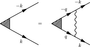
Figure 5: Ladder diagrams for the pairing vertex. The wavy line denotes the interaction mediated by spin fluctuations.

Because the pairing vertex is a spin singlet, $\Phi_{\alpha\beta}(k)=i\sigma_{\alpha\beta}^{y}\Phi(k)$. We denote by $\Phi_{0}(k)$ and $\Phi_{Q}(k)$ the pairing vertices with momenta near ${\bf k}$ and ${\bf k}+{\bf Q}$, respectively, and treat $k$ as a small deviation from the corresponding hot spot. Each ladder diagram renormalizes the pairing vertex by $\int_{q}G(q)G(-q)\chi(k-q+Q)$, where $\sum_{q}=T\sum_{\omega^{\prime}_{m}}\int d^{2}q/(2\pi)^{2}$ and $Q=({\bf Q},0)$ in 3D notations. The ladder diagrams are readily summed up and at $T=T_{c}$ give rise to the integral equation for $\Phi(k)$ in the form

$$\Phi_{0}(k)=-3g^{2}\sum_{q}\Phi_{\bf Q}(q)G(q)G(-q)\chi(k-q+Q).$$ (31)

where $\chi$ is given by Eq. (9). The overall factor $3$ comes from the convolutions of Pauli matrices at each vertex $\sigma_{\alpha^{\prime}\beta^{\prime}}^{y}\sigma_{\alpha\alpha^{\prime}}^{i}\sigma_{\beta\beta^{\prime}}^{i}=-3\sigma_{\alpha\beta}^{y}$, and the overall minus sign reflects the repulsive nature of the interaction. Superconducting instability is then possible only when $\Phi_{0}(k)=-\Phi_{\bf Q}(k)$. The spin singlet nature of pairing requires $\Phi(k)$ to be even function of the actual 2D momentum, which in our notations implies that $\Phi_{0}({\bf k},{\omega_{m}})=\Phi_{\bf Q}(-{\bf k},{\omega_{m}})$. Combined with $\Phi_{0}({\bf k},{\omega_{m}})=-\Phi_{\bf Q}({\bf k},{\omega_{m}})$, this requires $\Phi_{0}({-\bf k},{\omega_{m}})=-\Phi_{0}({\bf k},{\omega_{m}})$ and the same for $\Phi_{Q}$. Obviously then, the pairing amplitude passes through zero along the diagonals, i.e., the pairing symmetry is $d$-wave. For simplicity, below we replace $\Phi_{0}(k)$ by $\Phi(k)$ and $\Phi_{\bf Q}(k)$ by $-\Phi(k)$ and treat $\Phi(k)$ as an odd function of momentum (which, we remind, is counted from the corresponding hit spot along the diagonal). With this substitution, there will be no minus sign in the r.h.s. of the gap equation.

To simplify the calculation, we introduce the same set of rescaled dimensionless momenta and frequencies as before [Eq. (14)], and also rescale the temperature:

$$q\rightarrow\frac{\bar{g}\tilde{q}}{v_{F}\pi\lambda},~{}~{}~{}{\omega_{m}}\rightarrow\frac{\bar{g}\tilde{\omega}_{m}}{\pi\lambda},~{}~{}~{}\tilde{T}=\frac{\pi T\lambda}{\bar{g}}$$ (32)

In the new variables we have, instead of (31),

$$\Phi({\bf\tilde{k}},\tilde{\omega}_{m})=$$

$$\frac{3\lambda}{4\pi}\tilde{T}\sum_{\tilde{\omega}_{m}^{\prime}}\int\frac{d{\bf\tilde{q}}}{\tilde{\omega}_{m}^{\prime 2}+\tilde{q}_{x}^{2}}\chi^{(0)}({\bf\tilde{k}}-{\bf\tilde{q}},\tilde{\omega}_{m}-\tilde{\omega}_{m}^{\prime})\Phi({\bf\tilde{q}},\tilde{\omega}_{m}^{\prime})$$ (33)

where

$$\chi^{(0)}({\bf\tilde{k}}-{\bf\tilde{q}},\tilde{\omega}_{m}-\tilde{\omega}_{m}^{\prime})=$$

$$\frac{1}{({\bf\tilde{k}-\tilde{q}})^{2}+\sum_{a=\pm 1}\tilde{\Pi}^{(0)}_{a}({\bf\tilde{k}-\tilde{q}},{\tilde{\omega}_{m}}-{\tilde{\omega}_{m}}^{\prime})}.$$ (34)

As we did before, we have shifted ${\tilde{q}}_{x}$ by $\lambda^{2}{\tilde{q}}^{2}_{y}$ in (33) and dropped $\lambda^{2}$ terms in the spin susceptibility $\chi^{(0)}$. To simplify the presentation, below we will drop the tilde from the intermediate momentum and frequencies.

We focus our attention on the pairing between fermions in regions 1 and 4. The corresponding pairing vertex is an odd function of $k_{y}$ (the momentum component along the FS at a hot spot). For small $k_{y}$, we approximate the pairing vertex by $\Phi({\bf k},{\omega^{\prime}_{m}})=k_{y}\Phi(k_{x},{\omega^{\prime}_{m}})$. The only other place in (33) where the dependence on $k_{y}$ is present is the spin susceptibility. However, it depends only on the relative momentum transfer ${\bf k}-{\bf q}$ and is even function of the latter. In this situation, the integration over $q_{y}$ gives the result proportional to $k_{y}$, consistent with our approximation that $\Phi({\bf k},{\omega_{m}})=k_{y}\Phi(k_{x},{\omega_{m}})$. In explicit form, we have

$$\Phi(k_{x},{\omega_{m}})=$$

$$\frac{3\lambda}{4\pi}\tilde{T}\sum_{\omega_{m}^{\prime}}\int\frac{dq_{x}~{}\chi^{(0)}(k_{x}-q_{x},\omega_{m}-\omega_{m}^{\prime})}{\omega_{m}^{\prime 2}+q_{x}^{2}}\Phi(q_{x},\omega_{m}^{\prime})$$ (35)

where

$$\chi^{(0)}(k_{x}-q_{x},{\omega_{m}}-\omega_{m}^{\prime})=$$

$$\int\frac{dk_{y}}{k_{y}^{2}+(k_{x}-q_{x})^{2}+\sum_{a=\pm 1}\tilde{\Pi}^{(0)}_{a}(k_{x}-q_{x},k_{y},{\omega_{m}}-\omega_{m}^{\prime})}.$$ (36)

The function $\chi^{(0)}(k_{x}-q_{x},\omega_{m}-\omega_{m}^{\prime})$ plays the role of the pairing kernel. Like for electron-phonon systems, it tends to a finite value when $k_{x}-q_{x}$ and $\omega_{m}-\omega^{\prime}_{m}$ vanish:

$$\chi^{(0)}\equiv\int_{-\infty}^{\infty}\frac{dk_{y}}{k_{y}^{2}+\sqrt{|k_{y}|/2}}=\frac{2^{10/3}\pi}{3^{3/2}}=6.09.$$ (37)

To obtain the exponential term in $T_{c}$, we can just pull this constant out of $\tilde{T}\sum_{\omega_{m}^{\prime}}\int dq_{x}$ and evaluate the rest to logarithmical accuracy. We obtain

$$T_{c}\propto e^{-\frac{4\pi}{3\lambda\chi^{(0)}}}=e^{-\frac{0.6874}{\lambda}}.$$ (38)

To find the contribution from the ladder diagram to the prefactor, we use the same strategy as for electron-phonon case (see Appendix A) and write

$$\chi^{(0)}(k_{x}-q_{x} ,\omega_{m}-\omega_{m}^{\prime})=$$

$$\chi^{(0)}(k_{x},{\omega_{m}})+\delta\chi^{(0)}(k_{x},q_{x};\omega_{m},\omega_{m}^{\prime}),$$ (39)

where $\delta\chi^{(0)}(k_{x},0;\omega_{m},0)=0$. Substituting into Eq. (35), we obtain

$$\Phi(k_{x},{\omega_{m}})=\frac{3\lambda}{4\pi}\tilde{T}\sum_{\omega_{m}^{\prime}}\int dq_{x}\frac{1}{\omega_{m}^{\prime 2}+q_{x}^{2}}\times$$

$${\left[\chi^{(0)}(k_{x},{\omega_{m}})+\delta\chi^{(0)}(k_{x},q_{x};\omega_{m},\omega_{m}^{\prime})\right]}\Phi(\omega_{m}^{\prime},q_{x})$$ (40)

Of the two terms in the last line, the first one contains ${\lambda}\log\tilde{T}\sim O(1)$, while the second one (with $\delta\chi^{(0)}(k_{x},q_{x};\omega_{m},\omega_{m}^{\prime})$) is convergent in the infra-red limit and is of order of $\lambda$. The structure on the r.h.s. is reproduced on the l.h.s. if we take the pairing vertex in the form

$$\Phi(k_{x},{\omega_{m}})=\Phi^{0}\left[\chi^{(0)}(k_{x},{\omega_{m}})+\lambda\delta\Phi(k_{x},{\omega_{m}})\right]$$ (41)

Substituting this form back into the Eq. (35) for $\Phi$, we obtain

$$\chi^{(0)}(k_{x},{\omega_{m}})+\lambda\delta\Phi(k_{x},{\omega_{m}})$$

$$=\frac{3\lambda}{4\pi}\tilde{T}\sum_{\omega_{m}^{\prime}}\int dq_{x}~{}\frac{\chi^{(0)}(k_{x},\omega_{m})+\delta\chi^{(0)}(k_{x},q_{x};\omega_{m},\omega_{m}^{\prime})}{q^{2}_{x}+\omega_{m}^{\prime 2}}~{}\left[\chi^{(0)}(q_{x},\omega_{m}^{\prime})+\lambda\delta\Phi(q_{x},{\omega^{\prime}_{m}})\right]$$

$$=\frac{3\lambda^{2}}{4\pi}\tilde{T}\sum_{\omega_{m}^{\prime}}\int dq_{x}\frac{\chi^{(0)}(k_{x},\omega_{m})}{q^{2}_{x}+\omega_{m}^{\prime 2}}\delta\Phi(q_{x},{\omega^{\prime}_{m}})+\frac{3\lambda}{4\pi}\tilde{T}\sum_{\omega_{m}^{\prime}}\int dq_{x}\frac{\chi^{(0)}(q_{x},\omega_{m}^{\prime})\chi^{(0)}(k_{x}-q_{x},\omega_{m}-\omega_{m}^{\prime})}{q^{2}_{x}+\omega_{m}^{\prime 2}}+O(\lambda^{2})$$ (42)

To order $\lambda$ we then have

$$\delta\Phi(k_{x},\omega_{m})=\chi^{(0)}(k_{x},\omega_{m})\left[P+R(k_{x},\omega_{m})\right],$$ (43)

where

$$P =\frac{3\lambda}{4\pi}\tilde{T}\sum_{\omega_{m}^{\prime}}\int dq_{x}\frac{\delta\Phi(q_{x},{\omega_{m}^{\prime}})}{q^{2}_{x}+\omega_{m}^{{}^{\prime}2}},$$ (44)

$$R(k_{x},\omega_{m}) =\frac{3}{4\pi}\tilde{T}\sum_{\omega_{m}^{\prime}}\int dq_{x}\frac{\chi^{(0)}(q_{x},\omega_{m}^{\prime})\chi^{(0)}(k_{x}-q_{x},\omega_{m}-\omega_{m}^{\prime})}{\chi^{(0)}(k_{x},\omega_{m})\left(q^{2}_{x}+\omega_{m}^{\prime 2}\right)}-\frac{1}{\lambda}$$ (45)

Substituting Eq. (43) into the r.h.s. of Eq. (44) we obtain

$$\left[1-\frac{3\lambda}{4\pi}\tilde{T}\sum_{\omega^{\prime}_{m}}\int dq_{x}\frac{\chi^{(0)}(q_{x},\omega_{m}^{\prime})}{q^{2}_{x}+\omega_{m}^{\prime 2}}\right]P=\frac{3\lambda}{4\pi}\tilde{T}\sum_{\omega_{m}^{\prime}}\int dq_{x}\frac{\chi^{(0)}(q_{x},{\omega_{m}^{\prime}})}{q^{2}_{x}+\omega_{m}^{{}^{\prime}2}}R(q_{x},{\omega_{m}^{\prime}})$$ (46)

We now use the fact that $P=O(1)$, while the expression in the bracket of l.h.s. is of order $O(\lambda)$. The l.h.s. of (46) is then of $O(\lambda)$. The r.h.s. is $R(0,0)(1+O(\lambda))$. Obviously then $R(0,0)=O(\lambda)$, i.e.,

$$\frac{3\lambda\chi^{(0)}}{4\pi}\tilde{T}\sum_{\omega_{m}^{\prime}}\int dq_{x}\frac{\left[\chi^{(0)}(q_{x},\omega_{m}^{\prime})/\chi^{(0)}\right]^{2}}{\left(q^{2}_{x}+\omega_{m}^{\prime 2}\right)}$$

$$=1+O(\lambda^{2})$$ (47)

Evaluating the integral over $q_{x}$ and the sum over Matsubara frequencies, we obtain

$$\frac{4\pi}{3\chi^{(0)}}=\lambda\log\frac{0.00874}{\tilde{T}_{c}}+O(\lambda^{2})$$ (48)

or, in original notations, $T_{c}=T_{c1}$ from ladder diagrams is

$$T_{c1}=0.00249~{}\frac{\bar{g}}{\lambda}~{}e^{-\frac{0.6874}{\lambda}}$$ (49)

IV.2 The effect of fermionic self-energy

The self-energy corrections to ladder diagrams can be easily incorporated because in the FL regime their only role is to renormalize the quasiparticle $Z$, the Fermi velocity $v_{F}$, and the FS curvature $\kappa$. All three renormalizations can be absorbed into the renormalization of $\lambda$

$$\lambda=\left(\frac{\bar{g}\kappa}{2\pi v_{F}}\right)^{1/3}\rightarrow\left(\frac{\bar{g}Z^{2}\kappa^{*}}{2\pi v^{*}_{F}}\right)^{1/3}=\lambda(1-0.95\lambda).$$ (50)

Substituting this renormalization into Eq. (49) we obtain

$$T_{c2}=0.00130~{}\frac{\bar{g}}{\lambda}~{}e^{-\frac{0.6874}{\lambda}}$$ (51)

If Eliashberg theory was applicable to our problem, this would be the full result for $T_{c}$. However, as we already discussed, in our case Eliashberg parameter is of order one, and other renormalizations also play a role. Specifically, there are two extra contributions: from vertex corrections to the polarization operator and from Kohn-Luttinger renormalization of the irreducible pairing interaction. The two contributions add up and we consider them separately.

IV.3 Correction to $T_{c}$ due to the renormalization of the polarization operator

The exponential factor in the expressions for $T_{c1}$ and $T_{c2}$ is proportional to the integral

$$\chi^{(0)} =\int dq_{y}\chi(q_{x}=0,q_{y},\omega_{m}=0)$$

$$=\int dq_{y}\frac{1}{q^{2}_{y}+\sum_{a=\pm 1}\tilde{\Pi}^{(0)}_{a}(0,q_{y},0)}$$ (52)

In evaluating this integral, we used the free-fermion form of the polarization operator, in which case $\sum_{a=\pm 1}\tilde{\Pi}^{(0)}_{a}(0,q_{y},0)=\sqrt{|q_{y}|/2}$ and $\chi^{(0)}=6.09$. However, to get the prefactor in $T_{c}$, we need to know the exponential factor with accuracy $O(\lambda)$. Self-energy contributions to $\tilde{\Pi}^{(0)}_{a}(0,q_{y},0)$ are incorporated into the renormalization of $\lambda$ in (50) and are accounted for in Eq. (51). However, the vertex correction to $\tilde{\Pi}^{(0)}_{a}(0,q_{y},0)$ also contributes the term of order $\lambda$, and this term has to be included.

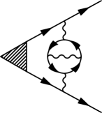
Figure 6: Ladder diagrams with the effective interaction which includes vertex correction to the polarization bubble.

The effective pairing interaction with vertex correction to the polarization bubble included is shown in FIG. 6. For a generic ${\bf q}$ and $\Omega_{m}$, the computation of the vertex renormalization is rather messy dan . For our purposes, however, we will only need vertex correction for a static polarization bubble at ${\bf q}=(0,q_{y})$, and only for umklapp process (i.e., in our case, the contribution to $\Pi$ from virtual fermions in hot region 3 and 2,

We present the computation of the vertex correction to $\Pi$ in Appendix B and here state the result – this renormalization changes $\chi^{(0)}$ by an $O(\lambda)$ term:

$$\chi^{(0)}\rightarrow\chi^{(0)}(1-0.042\lambda).$$ (53)

Including this renormalization into the expression for $T_{c}$, Eq. (49), we find

$$T_{c3}=0.00126~{}\frac{\bar{g}}{\lambda}~{}e^{-\frac{0.6874}{\lambda}}$$ (54)

IV.4 Kohn-Luttinger type corrections to effective interaction

Finally, we consider the effect on $T_{c}$ from Kohn-Luttinger type second-order corrections to the effective pairing interaction. We show the corresponding diagrams in FIG. 7. Compared to the original Kohn-Luttinger work kl , we have dropped one diagram since in our case it is already included into $\chi^{(0)}(k)$.

Figure 7: Kohn-Luttinger diagrams for the irreducible pairing interaction. The diagram with internal particle-hole bubble is already included into $\chi^{(0)}(k)$ and has to be dropped to avoid double counting. Each of the remaining three Kohn-Luttinger diagrams gives contribution of order $\lambda$.

Similar to what we did before with the dynamical part of the interaction in ladder series, we analyze the equation for the pairing vertex using the full $\chi$ which we split into the original and the Kohn-Luttinger terms. We have

$$\Phi({\bf k},\omega_{m})=\frac{3\lambda}{4\pi}\tilde{T}\sum_{\omega_{m}^{\prime}}\int\frac{d{\bf q}}{\omega_{m}^{\prime 2}+q_{x}^{2}}\chi({\bf k},\omega_{m};{\bf q},\omega_{m}^{\prime})\Phi({\bf q},\omega_{m}^{\prime})$$ (55)

where

$$\chi({\bf k},\omega_{m};{\bf q},\omega_{m}^{\prime})= \chi^{(0)}(k_{x}-q_{x},k_{y}-q_{y},\omega_{m}-\omega_{m}^{\prime})$$

$$+ {\lambda}\chi^{(1)}(k_{x},k_{y},\omega_{m};q_{x},q_{y},\omega_{m}^{\prime});$$ (56)

$\chi^{(0)}(k-q)$, defined in Eq. (34), accounts for the first graph in FIG. 7, and ${\lambda}\chi^{(1)}(k,q)$ accounts for the other three terms.

The first term in $\chi(k,q)$ depends on the momentum transfer $k_{y}-q_{y}$. For this reason we could shift, in the r.h.s. of (50), the integration over $q_{y}$ by the integral over $q_{y}-k_{y}$ and obtain the pairing vertex as a linear function of $k_{y}$. This simple scaling with $k_{y}$ does not extend to Kohn-Luttinger terms because $\chi^{(1)}(k,q)$ depends separately on $k$ and on $q$. Accordingly, we write

$$\Phi(k_{x},k_{y},{\omega_{m}})=\Phi^{0}[k_{y}\chi^{(0)}(k_{x},{\omega_{m}})+\lambda\delta\Phi(k_{x},k_{y},{\omega_{m}})].$$ (57)

Because we are interested in $O(\lambda)$ terms, we can safely neglect the difference between continuous and discrete Matsubara frequencies and treat $\omega_{m}$ as continuous variable.

Plugging (57) back to the pairing equation and formally setting $k_{x}={\omega_{m}}=0$, we obtain

$$k_{y}\chi^{(0)}+\lambda\delta\Phi(0,k_{y},0) =\frac{3\lambda}{4\pi}\tilde{T}\sum\int\frac{dq_{x}}{({\omega^{\prime}_{m}})^{2}+q_{x}^{2}}k_{y}\left(\chi^{(0)}(q_{x},\omega_{m}^{\prime})\right)^{2}$$

$$+\frac{3\lambda^{2}}{4\pi}\tilde{T}\sum\int\frac{dq_{x}}{({\omega^{\prime}_{m}})^{2}+q_{x}^{2}}\int dq_{y}\chi^{(1)}(0,k_{y},0;q_{x},q_{y},\omega_{m}^{\prime})q_{y}\chi^{(0)}(q_{x},\omega_{m}^{\prime})$$

$$+\frac{3\lambda^{2}}{4\pi}\tilde{T}\sum\int\frac{dq_{x}}{({\omega^{\prime}_{m}})^{2}+q_{x}^{2}}\int dq_{y}\chi^{(0)}(q_{x},k_{y}-q_{y},\omega_{m}^{\prime})\delta\Phi(q_{x},q_{y},\omega_{m}^{\prime})$$

Evaluating the integrals, we obtain

$$k_{y}\chi^{(0)}+\lambda\delta\Phi(0,k_{y},0) =k_{y}\frac{3\lambda}{4\pi}\chi^{(0)2}\log{\frac{0.00874}{{\tilde{T}}}}+\frac{3\lambda^{2}}{4\pi}\chi^{(0)}\log\frac{a}{\tilde{T}}\int dq_{y}\chi^{(1)}(0,k_{y},0;0,q_{y},0)q_{y}$$

$$+\frac{3\lambda^{2}}{4\pi}\log\frac{{b}}{\tilde{T}}\int dq_{y}\chi^{(0)}(0,k_{y}-q_{y},0)\delta\Phi(0,q_{y},0)+O(\lambda^{2}).$$ (59)

where $a$ and $b$ are constants of order one.

Simplifying the notations and rearranging, we re-express (59) as

$$\frac{4\pi}{3\lambda\chi^{(0)}}=\log{\frac{0.00874}{\tilde{T}}}+\frac{A(k_{y})+C(k_{y})}{k_{y}(\chi^{(0)})^{2}}+O(\lambda^{2}).$$ (60)

where we defined

$$A(k_{y}) =\int dq_{y}\left[\frac{\chi^{(0)}(k_{y}-q_{y})}{\chi^{(0)}}\delta\Phi(0,q_{y},0)\right]-\delta\Phi(0,k_{y},0)$$

$$C(k_{y}) =\int dq_{y}q_{y}\chi^{(1)}(0,k_{y},0;0,q_{y},0)$$ (61)

and $\chi^{(0)}(k_{y}-q_{y})=1/[(k_{y}-q_{y})^{2}+\sqrt{|k_{y}-q_{y}|/2}]$. One can easily make sure that $A(0)=C(0)=0$, hence $[A(k_{y})+\xi^{(1)}(k_{y})]/k_{y}$ is not singular when $k_{y}$ vanishes. However, Eq. (59) sets a more stringent requirement: $A(k_{y})+C(k_{y})$ must be equal to $Bk_{y}(\chi^{(0)})^{2}$, where $B$ is a constant. Then $T_{c}=T_{c3}e^{B}$, where $T_{c3}$ is given by Eq. (54).

The $A(k_{y})$ in Eq. (61) contains $\delta\Phi(0,k_{y},0)$ and the integral over $q_{y}$ of $\delta\Phi(0,y_{y},0)$, weighted with a kernel. The condition

$$A(k_{y})+C(k_{y})=Bk_{y}(\chi^{(0)})^{2}$$ (62)

then sets the integral equation on $\delta\Phi(0,k_{y},0)$. We solve this equation in Appendix C and obtain $B$ in the form $B=C(-\Lambda)/(\chi^{(0)})^{2}$, where $\Lambda$ is the dimensionless momentum cutoff along the FS.

The value of $B$ depends on the interplay between $\lambda$ and $1/\Lambda$. For a generic FS, the momentum cutoff $\Lambda$ is of order $k_{F}$, in which case $\lambda\Lambda\sim(W/{\bar{g}})^{1/3}\gg 1$, where $W$ is fermionic bandwidth. In this situation, the pairing interaction dies off at momenta $k_{y}$, which are parametrically smaller than the cutoff, and and $C(-\Lambda)$ is small in $1/(\lambda\Lambda)$. Then $B$ is also small in $1/(\lambda\Lambda)$, hence $e^{B}\approx 1$, i.e., the correction to $T_{c}$ from Kohn-Luttinger diagrams can be neglected. In this situation, the fully renormalized $T_{c}$ coincides with $T_{c3}$ and is given by

$$T_{c}=0.00126~{}\frac{\bar{g}}{\lambda}~{}e^{-\frac{0.6874}{\lambda}}$$ (63)

Equation (63) is the main result of this paper.

If, by some reasons, $\Lambda$ is numerically much smaller than $k_{F}$, such that $\lambda\Lambda$ is actually a small number, the renormalization of $T_{c}$ due to Kohn-Luttinger diagrams becomes relevant. We present the calculation of $B$ for this case in Appendix C. We find that, at small $\lambda\Lambda$, $B$ is logarithmically singular: $B=(10/3)\log{1/(\lambda\Lambda)}+...$ where the ellipsis stand for terms $O(1)$. As a result, $T_{c}$ is enhanced by the factor $(1/\lambda\Lambda)^{10/3}$ compared to Eq. (63). The outcome is that Eq. (63) provides the lower boundary for $T_{c}$ – the actual $T_{c}$ gets enhanced by Kohn-Luttinger contributions. How strong the enhancement is depends on the actual band structure, which set the value of $\Lambda$.

IV.5 Comparison with the experiments on electron-doped cuprates

We now compare our theoretical $T_{c}$, Eq. (63), with the data for near-optimally doped ${\rm Nd}_{2-x}{\rm Ce}_{x}{\rm Cu}_{3}{\rm O}_{4}$  and ${\rm Pr}_{2-x}{\rm Ce}_{x}{\rm Cu}_{3}{\rm O}_{4}$, in which doping creates extra electrons. The parameters of the quasiparticle dispersion, $v_{F}$ and $\kappa$, can be extracted from the ARPES measurements on ${\rm Nd}_{2-x}{\rm Ce}_{x}{\rm Cu}_{3}{\rm O}_{4}$ exp_el . We found $v_{F}=0.87\rm eV$ and $\kappa=0.31$ (in units where the lattice constant $a=1$). Similar parameters have been obtained in  mar_fit . The only other input parameter for the theory is the strength of spin-fermion coupling ${\bar{g}}$. For hole-doped cuprates, the fits to ARPES and NMR data in the normal state yielded ${\bar{g}}\leq 2\rm eV$ (Ref. [acs, ]). This ${\bar{g}}$ is consistent with the value of the charge-transfer gap in the effective Hubbard model in the Mott-Heisenberg regime at half-filling opt_1/2_hole as calculations in the ordered state of the spin-fermion model morr place the gap to be exactly ${\bar{g}}$ – quantum corrections cancel out. This consistency is not an anticipated result as ${\bar{g}}$ extracted from the optics is the coupling at high-energies, comparable to $E_{F}$, while the one used in the comparison with ARPES and NMR is the coupling at low-energies (below our $\Lambda$), where, strictly speaking, spin-fermion model is only valid. The (rough) agreement between the two likely implies that renormalizations between $E_{F}$ and $\Lambda$ do reduce ${\bar{g}}$, but only by a small fraction. For electron-doped cuprates, the detailed fits of $\Sigma(k,\omega)$ in the spin-fermion model to the self-energy, extracted from ARPES data, have not been done yet, but optical measurements optics_el show that the charge-transfer gap is about $1.7\rm eV$. Assuming that the situation in electron-doped cuprates is the same as in hole-doped cuprates, i.e., that spin-fermion couplings, extracted from ARPES and optics, are not far each other, we just take ${\bar{g}}$ to be equal to this $1.7\rm eV$.

Using the numbers for ${\bar{g}}$, $v_{F}$, and $\kappa$, we obtain $\lambda\sim 0.46$, which implies that weak coupling analysis should be applicable. Substituting $\lambda=0.46$ and ${\bar{g}}\approx 20000\rm K$, we find $T_{c}\sim 0.0006{\bar{g}}\sim 12\rm K$. This is reasonably close to the experimental $T_{c}=20-24\rm K$ in optimally doped ${\rm Nd}_{2-x}{\rm Ce}_{x}{\rm Cu}_{3}{\rm O}_{4}$  takagi ; TC2 particularly given that our theoretical $T_{c}$, Eq. (63) is the lower boundary for the actual $T_{c}$ because (i) as we found above, $T_{c}$ goes up once we include corrections due to a finite upper cutoff of the theory, and (ii) in real situation, hot spots at optimal doping are still located at some distance from each other, in which case the value of $T_{c}$ should move a bit towards the one when hot spots are well separated, and the latter is much higher: when hot spots are near $(0,\pi)$ and symmetry-related points, $T_{c}\sim 0.04{\bar{g}}$  wang ; norman_1 .

The transition temperature in the similar range of $10-20\rm K$ has been found in FLEX calculations FLEX , and the agreement between our and FLEX results in an encouraging sign. The authors of  mar_fit ; bansil considered the model with a static interaction $V$, extracted $V$ by fitting the value of the magnetization in the antiferromagnetically ordered state, and used BCS formula for $T_{c}$. Amazingly, their $T_{c}$ is quite similar to the one we obtained. The two-particle-self-consistent approach, applied to the Hubbard model with nearest-neighbor hopping only and values of the interaction $U$ typical of electron-doped systems, yields a much higher optimal $T_{c}\sim 200\rm K$ [Refs. tremblay, ; X, ]. However, given the sensitivity of $T_{c}$ to the specifics of the FS XX , the value of $T_{c}$ in this approach has to be reanalyzed using the model for the hopping consistent with the measured FS.

V Summary

In this work, we re-visited the issue of normal state renormalizations and superconducting $T_{c}$ in electron-doped cuprates near optimal doping. We used spin-fermion model to model electronic interactions and assumed that the doping at which magnetic order with ${\bf Q}=(\pi,\pi)$ sets in is close to the one at which the Fermi surface touches the magnetic Brillouin zone boundary along the zone diagonals (this case is often labeled as ${\bf Q}=2{\bf k}_{F}$).

Quantum-critical fluctuations and the pairing instability in the ${\bf Q}=2{\bf k}_{F}$ case have been studied before aim_el ; krotkov . However, recent work subir_el has shown that earlier analysis did not include umklapp processes and, as a result, severely overestimated the strength of quantum-critical fluctuations. Once umklapp process are properly accounted for, the real part of the self-energy at a QCP scales as $\omega$ and the imaginary part behaves as $\omega^{3/2}\log{\omega}$, i.e., fermionic coherence is preserved at the lowest energies.

The goal of this work was to re-visit the calculation of $T_{c}$. We found that the argument krotkov that the $d_{x^{2}-y^{2}}$ superconductivity survives when hot spots merge along Brillouin zone diagonals, holds. However, the value of $T_{c}$ has to be re-considered. The calculation of $T_{c}$ requires one to know the renormalization of the quasiparticle propagator in the normal state, and in the first part of the paper we computed the real part of the fermionic self-energy (which was not considered in Ref. subir_el ). We found that Eliashberg approximation is not valid because the Eliashberg parameter is of order one, and the only way to proceed with calculations is to perform a direct perturbative loop expansion. We found that Re $\Sigma(k,\omega)$ is a regular function of momentum and frequency, and the renormalizations of the quasiparticle residue $Z$, Fermi velocity $v_{F}$, and the FS curvature $\kappa$ hold on powers of the single dimensionless parameter $\lambda$. We treated $\lambda$ as small parameter and obtained $Z$, $v_{F}$, and $\kappa$ to order $O(\lambda)$.

We then used normal state results as an input and computed superconducting $T_{c}$ by solving the (2+1)-dimensional gap equation in momentum and frequency. To logarithmical accuracy, the solution of the linearized gap equation is similar to that in BCS theory, and $T_{c}\propto e^{-a/\lambda}$, where in our case $a=0.6874$. We, however, computed $T_{c}$ with the prefactor, which required us to go one step beyond BCS approximation and include the frequency dependence of the interaction, the renormalizations of $Z$, $v_{F}$, and $\kappa$, vertex corrections to particle-hole polarization bubble, and Kohn-Luttinger (non-ladder) corrections to the irreducible pairing interaction. Using the parameters extracted from the data on optimally electron-doped cuprates, we found $T_{c}\geq 10\rm K$, which is in a reasonably good agreement with the experimental values. The agreement is particularly striking because our result is the lower boundary of the actual $T_{c}$.

One issue brought about by our work in comparison with earlier works on the Hubbard model tremblay ; tremblay_1 ; X ; XX is the origin of the difference between hole and electron-doped cuprates. The reasoning displayed in tremblay ; tremblay_1 ; X ; XX ; gabi is that the interaction $U$ is somewhat smaller in electron-doped cuprates than in hole-doped cuprates such that in electron-doped materials correlations are relevant, but Mott physics does not develop. This is certainly a valid point as, e.g., the magnetic $T_{N}$ is smaller in half-filled ${\rm Pr}_{2-x}{\rm Ce}_{x}{\rm Cu}_{3}{\rm O}_{4}$,and ${\rm Pr}_{2-x}{\rm Ce}_{x}{\rm Cu}_{3}{\rm O}_{4}$ than in undoped La and Y based materials). Our results, however, point on a complementary reason for the difference between near-optimally hole and electron-doped cuprates. Namely, even if interaction (our ${\bar{g}}$) is the same, there is still a substantial difference between the magnitude of fermionic self-energy and of superconducting $T_{c}$ due to the difference in the geometry of the electronic FS.

Appendix A $T_{c}$ at weak coupling in a phonon superconductor

A portion of our calculation of $T_{c}$ is similar to the calculation of $T_{c}$ in the weak-coupling limit of Eliashberg theory for a phonon superconductor for the case when a phonon propagator can be approximated by a single Einstein mode:

$$\chi_{ph}(\Omega_{m})=\frac{\chi_{0}}{\Omega^{2}_{m}+\omega^{2}_{D}}$$ (64)

In Eliashberg theory, $T_{c}$ is the temperature at which the linearized equation for the pairing vertex $\Phi(\Omega_{m})$ has a non-zero solution. The equation for $\Phi(\Omega_{m})$ is well-known phonons ; phonons_1 ; phonons_2 ; phonons_3 and in rescaled variables ${\bar{T}}=T/\omega_{D}$, ${\bar{\omega}}_{m}=\omega_{m}/\omega_{D}=\pi{\bar{T}}(2m+1)$ reads

$$\Phi({\bar{\Omega}}_{m})=\pi{\bar{T}}\lambda^{*}\sum_{m}\frac{\Phi({\bar{\omega}}_{m})}{|{\bar{\omega}}_{m}|}\chi(\bar{\omega}_{m},\bar{\Omega}_{m})$$ (65)

where $\chi(\bar{\omega}_{m},\bar{\Omega}_{m})\equiv\frac{1}{1+\left({\bar{\omega}}_{m}-{\bar{\Omega}}_{m}\right)^{2}}$ and $\lambda^{*}=\lambda/(1+\lambda)$ [$\lambda$ is dimensionless effective electron-phonon coupling and the factor $(1+\lambda)$ comes from mass renormalization] The formula for $T_{c}$ in Eliashberg theory at weak coupling has been discussed several times in the past phonons_1 ; phonons_2 ; phonons_3 . However, until now, there is some confusion about the interplay between the weak coupling limit of the Eliashberg theory and the BCS theory phonons . Within BCS theory (extended to include $1+\lambda$ mass renormalization), the pairing vertex is approximated by a constant and the dependence on the external ${\bar{\Omega}}_{m}$ in the bosonic propagator is neglected. The equation for $T_{c}$ then reduces to

$$1=\lambda^{*}\sum_{m}\frac{1}{|2m+1|}\frac{1}{1+\pi^{2}{\bar{T}}^{2}(2m+1)^{2}}$$ (66)

The sum in the r.h.s. converges at the largest $m$ and is expressed in terms of di-Gamma functions. At small ${\bar{T}}$ it reduces to $\log{1.13/{\bar{T}}}$. From (67) we then obtain, in original notations,

$$T^{BCS}_{c}=1.13\omega_{D}e^{-\frac{1+\lambda}{\lambda}}$$ (67)

The point made in Refs.phonons_1 ; phonons_2 ; phonons_3 is that this expression is not the correct $T_{c}$ in the small $\lambda$ limit of the Eliashberg theory. The correct formula, obtained first in Ref. phonons_1 (see also phonons_2 ; phonons_3 ), is

$$T_{c}=1.13e^{-1/2}\omega_{D}e^{-\frac{1+\lambda}{\lambda}}=0.69\omega_{D}e^{-\frac{1+\lambda}{\lambda}}$$ (68)

The reason for the discrepancy between Eqs. (67) and (68) is that in Eliashberg theory the numerical prefactor in $T_{c}$ comes from fermions with energies of order $\omega_{D}$ (${\tilde{\omega}}_{m}=O(1)$), and for such fermions the dependence of the pairing vertex $\Phi({\bar{\omega}}_{m})$ on ${\bar{\omega}}_{m}$ cannot be neglected.

The computational procedure presented in Ref. phonons_1 and in subsequent work phonons_3 uses iteration method and is somewhat involved. Below we present an alternative computation procedure to obtain Eq. (68). We use the same procedure in the calculations of $T_{c}$ for our case of electron-doped cuprates. We re-express $\chi(\bar{\omega}_{m},\bar{\Omega}_{m})\equiv\frac{1}{1+\left({\bar{\omega}}_{m}-{\bar{\Omega}}_{m}\right)^{2}}$ in Eq. (65) as

$$\chi(\bar{\omega}_{m},\bar{\Omega}_{m}) \equiv\chi(\bar{\Omega}_{m})+\delta\chi(\bar{\omega}_{m},\bar{\Omega}_{m})$$

$$\chi(\bar{\Omega}_{m}) =\frac{1}{1+{\bar{\Omega}}^{2}_{m}}$$

$$\delta\chi(\bar{\omega}_{m},\bar{\Omega}_{m}) =\frac{\bar{\omega}_{m}}{1+{\bar{\Omega}}^{2}_{m}}\frac{2{\bar{\Omega}}_{m}-{\bar{\omega}}_{m}}{1+\left({\bar{\omega}}_{m}-{\bar{\Omega}}_{m}\right)^{2}}.$$ (69)

Plugging this expression back to Eq. (65) we find that the first term in Eq. (69) gives $\lambda^{*}\log\bar{T}\sim 1$, while the second term is free of logarithm and is of order $\lambda^{*}$. We then search for the solution of Eq. (65) in the form

$$\Phi({\bar{\Omega}}_{m})={\Phi_{0}}\left[\chi(\bar{\Omega}_{m})+\lambda^{*}\delta\Phi(\bar{\Omega}_{m})\right]+O(\lambda^{*2}),$$ (70)

where $\delta\Phi({\bar{\Omega}}_{m})$ is assumed to be independent of $\lambda^{*}$ up to corrections of order $\lambda^{*}$. Substituting Eq. (70) into Eq. (65) and neglecting non-logarithmical terms of order $(\lambda^{*})^{2}$, we obtain

$$\delta\Phi({\bar{\Omega}}_{m})=\chi({\bar{\Omega}}_{m})\left[P+R({\bar{\Omega}}_{m})\right],$$ (71)

where

$$P =\lambda^{*}\pi T_{c}\sum\frac{\delta\Phi({\bar{\omega}}_{m})}{|{\bar{\omega}}_{m}|}$$ (72)

$$R({\bar{\Omega}}_{m}) =\frac{\pi T_{c}}{\chi(\bar{\Omega}_{m})}\sum\frac{1}{|{\bar{\omega}}_{m}|}\chi(\bar{\omega}_{m})\chi(\bar{\omega}_{m},\bar{\Omega}_{m})-\frac{1}{\lambda^{*}}$$ (73)

Observe that Eq. (71) is not an integral equation on $\delta\Phi({\bar{\Omega}}_{m})$ because the integral term $P$ does not depend on ${\bar{\Omega}}_{m}$.

Constructing $P$ in the r.h.s. of Eq. (71), we obtain

$$\left[1-\lambda^{*}\pi\bar{T}_{c}\sum\frac{\chi(\bar{\omega}_{m})}{|\bar{\omega}_{m}|}\right]P=\lambda^{*}\pi\bar{T}_{c}\sum\frac{\chi(\bar{\omega}_{m})}{|\bar{\omega}_{m}|}R(\bar{\omega}_{m})$$ (74)

Because $1-\lambda^{*}\pi\bar{T}_{c}\sum\frac{1}{|\bar{\omega}_{m}|}\chi(\bar{\omega}_{m})=O(\lambda^{*})$ and $P$ is at most of order $O(1)$, the l.h.s. of Eq. (74) is $O(\lambda^{*})$. On the other hand, the r.h.s of Eq. (74) becomes

$$\lambda^{*}\pi\bar{T}_{c}\sum\frac{1}{|\bar{\omega}_{m}|}\chi(\bar{\omega}_{m})R(\bar{\omega}_{m})=R(0)\left(1+O(\lambda^{*})\right).$$ (75)

Matching both sides, we find that

$$R(0)=O(\lambda^{*}),$$ (76)

hence

$$\lambda^{*}\pi T_{c}\sum\frac{1}{|{\bar{\omega}}_{m}|}\frac{1}{\left(1+{\bar{\omega}}^{2}_{m}\right)^{2}}=1+O(\lambda^{*2})$$ (77)

Evaluating the sum (it is expressed in terms of di-Gamma functions) and taking the limit ${\bar{T}}\ll 1$, we reproduce Eq. (68).

Another way to obtain this result is to formally set $\bar{\Omega}_{m}=0$ in Eq. (71), which gives $\delta\Phi(0)=P+R(0)$. At the same time, from Eq. (72) we have $P=\delta\Phi(0)+O(\lambda^{*})$. Matching the two expressions, we reproduce $R(0)=O(\lambda^{*})$.

Appendix B Evaluation of the contribution to $T_{c}$ from vertex corrections to the polarization bubble

Figure 8: Vertex correction to polarization bubble. Labels $i$ and $j$ denotes fermions at different hot spots. The full expression is the sum of direct and umklapp processes, $(1,4),(4,1)$, $(2,3),(3,2)$.

In this Appendix we present the evaluation of the contribution to $T_{c}$ from vertex correction to the polarization bubble $\Pi^{(1)}({\bf q+Q},\Omega_{m})$.

The diagram for $\Pi^{(1)}({\bf q+Q},\Omega_{m})$ is shown in FIG. 8. As we discussed, vertex correction to the polarization bubble contributes to $T_{c}$ by renormalizing $\chi^{(0)}$. For our purposes, one can easily make sure that we only need to include the renormalization of the spin susceptibility and at transferred momentum ${\bf q}=(0,q_{y})$. For momentum along $y$ axis, the contribution from umklapp process dominates, because in direct process $q_{y}$ dependence is suppressed by $\lambda$. We denote the contribution from umklapp process at $\left(q_{x}=0,q_{y},\Omega_{m}=0\right)$ as $\Pi_{um}^{(1)}(0,q_{y},0)$. We have,

$$\Pi_{um}^{(1)} (0,q_{y},0)=-2\bar{g}^{2}\int\frac{d{\bf k}_{1}~{}d\omega_{m1}}{(2\pi)^{3}}\int\frac{d{\bf k}_{2}~{}d\omega_{m2}}{(2\pi)^{3}}\frac{1}{\left({\bf k}_{1}-{\bf k}_{2}\right)^{2}+\Pi\left({\bf k}_{1}-{\bf k}_{2},\omega_{m1}-\omega_{m2}\right)}$$

$$\times\frac{1}{i\omega_{m1}-\bar{\epsilon}_{k_{1}}}\frac{1}{i\omega_{m1}-\bar{\epsilon}_{-k_{1}+q}}\frac{1}{i\omega_{m2}-\bar{\epsilon}_{k_{2}}}\frac{1}{i\omega_{m2}-\bar{\epsilon}_{-k_{2}+q}}+\left({\bf q}\rightarrow-{\bf q}\right),$$ (78)

where

$$\bar{\epsilon}_{k}=v_{F}\left(k_{y}-\kappa\frac{k_{x}^{2}}{2}\right),$$ (79)

where the coefficient $(-2)$ comes from Pauli matrix algebra. Using a set of rescaling variables similar to the one introduced in Eq. (14) in the main text, we obtain

$$\Pi_{um}^{(1)}(0,q_{y},0)=\lambda\left(\frac{\bar{g}}{\pi v_{F}\lambda}\right)^{2}\tilde{\Pi}_{um}^{(1)}(0,\tilde{q}_{y},0),$$ (80)

where

$$\tilde{\Pi}_{um}^{(1)}(0,\tilde{q}_{y},0)= -4\pi^{2}\int\frac{du~{}dx~{}dy}{(2\pi)^{3}}\int\frac{dU~{}dX~{}dY}{(2\pi)^{3}}\frac{1}{X^{2}+Y^{2}+\sum_{a}\tilde{\Pi}_{a}^{(0)}(X,Y,U)}$$

$$\times \frac{1}{-i\left(u-\frac{U}{2}\right)+\left(y-\frac{Y}{2}+\frac{\tilde{q}_{y}}{2}\right)-x^{2}}\frac{1}{i\left(u-\frac{U}{2}\right)+\left(y-\frac{Y}{2}-\frac{\tilde{q}_{y}}{2}\right)+x^{2}}$$

$$\times \frac{1}{i\left(u+\frac{U}{2}\right)+\left(y+\frac{Y}{2}+\frac{\tilde{q}_{y}}{2}\right)+x^{2}}\frac{1}{-i\left(u+\frac{U}{2}\right)+\left(y+\frac{Y}{2}-\frac{\tilde{q}_{y}}{2}\right)-x^{2}}$$ (81)

Eq. (81) is a 6$D$ integral, for which numerical schemes designed to evaluate multidimensional integrals, such as Monte-Carlo, do not yield satisfactory results. Fortunately, the integration over $u,x$ and $y$, which are rescaled frequency and two momentum components in the fermionic loop, can be done analytically. The remaining integration over $U,X,Y$, can be done numerically to a good precision.

To perform the integration, we first write down

$$\tilde{\Pi}_{um}^{(1)}(0,\tilde{q}_{y},0)=-4\pi^{2}I(\tilde{q}_{y}),$$ (82)

where

$$I(\tilde{q}_{y})= \int\frac{dU~{}dX~{}dY}{(2\pi)^{3}}\int\frac{du~{}dx~{}dy}{(2\pi)^{3}}\frac{1}{X^{2}+Y^{2}+\sum_{a}\tilde{\Pi}_{a}^{(0)}(X,Y,U)}$$

$$\times \underbrace{\frac{1}{-i\left(u-\frac{U}{2}\right)+\left(y-\frac{Y}{2}+\frac{\tilde{q}_{y}}{2}\right)-x^{2}}}_{(1)}\underbrace{\frac{1}{i\left(u-\frac{U}{2}\right)+\left(y-\frac{Y}{2}-\frac{\tilde{q}_{y}}{2}\right)+x^{2}}}_{(2)}$$

$$\times \underbrace{\frac{1}{i\left(u+\frac{U}{2}\right)+\left(y+\frac{Y}{2}+\frac{\tilde{q}_{y}}{2}\right)+x^{2}}}_{(3)}\underbrace{\frac{1}{-i\left(u+\frac{U}{2}\right)+\left(y+\frac{Y}{2}-\frac{\tilde{q}_{y}}{2}\right)-x^{2}}}_{(4)}$$ (83)

We use the residue theorem for the integration over $dy$. There are four poles, from terms labeled (1) (2) (3) and (4). We split $I$ into two parts, $I(\tilde{q}_{y})=I_{1}(\tilde{q}_{y})+I_{2}(\tilde{q}_{y})$. $I_{1}$ comes from the range where the poles in (1) and (4) are in the same half plane, while $I_{2}$ comes from the range where the poles in (2) and (4) are in the same half plane.

For $I_{1}$ we obtain

$$I_{1}(\tilde{q}_{y}) =2\pi i\int\frac{dU~{}dX~{}dY}{(2\pi)^{3}}\int_{|u|>\frac{|U|}{2}}du~{}{\rm sgn}{(u)}\int\frac{dx}{(2\pi)^{3}}\frac{1}{X^{2}+Y^{2}+\sum_{a}\tilde{\Pi}_{a}^{(0)}(X,Y,U)}$$

$$\times\frac{1}{2x^{2}+Y+2iu}~{}\frac{1}{2x^{2}-{\tilde{q}_{y}}+2i\left(u-\frac{U}{2}\right)}~{}\frac{1}{-iU+Y-{\tilde{q}_{y}}}+\left({\tilde{q}_{y}}\rightarrow-{\tilde{q}_{y}}\right)$$ (84)

rearranging the second line and combining the integrals over positive and negative $u$, we obtain

$$I_{1}(\tilde{q}_{y}) =\int\frac{dU~{}dX~{}dY}{16\pi^{5}}\frac{1}{X^{2}+Y^{2}+\sum_{a}\tilde{\Pi}_{a}^{(0)}(X,Y,U)}\int_{\frac{|U|}{2}}^{\infty}du\int_{-\infty}^{\infty}dx$$

$$\times{\rm Im}\left\{\left[\frac{1}{2x^{2}+Y+2iu}-\frac{1}{2x^{2}-{\tilde{q}_{y}}+2i\left(u-\frac{U}{2}\right)}\right]\frac{1}{Y^{2}-({\tilde{q}_{y}}+iU)^{2}}\right\}+\left({\tilde{q}_{y}}\rightarrow-{\tilde{q}_{y}}\right)$$ (85)

We next perform the integration over $x$ and over $u$ using the same steps as we did in the calculation of the one-loop polarization bubble in the main text. Carrying out the integrations, we obtain

$$I_{1}(\tilde{q}_{y}) =-\int\frac{dU~{}dX~{}dY}{16\pi^{4}\sqrt{2}}\frac{1}{X^{2}+Y^{2}+\sum_{a}\tilde{\Pi}_{a}^{(0)}(X,Y,U)}$$

$$\times{\rm Re}\left[\left(\sqrt{Y+i|U|}-\sqrt{-{\tilde{q}_{y}}-iU+i|U|}\right)\frac{1}{Y^{2}-({\tilde{q}_{y}}+iU)^{2}}\right]+\left({\tilde{q}_{y}}\rightarrow-{\tilde{q}_{y}}\right)$$ (86)

Folding the integration over $U$ to positive $U$, we re-write (86) as

$$I_{1}(\tilde{q}_{y}) =\int_{0}^{\infty}dU\int\frac{dX~{}dY}{16\pi^{4}\sqrt{2}}\frac{1}{X^{2}+Y^{2}+\sum_{a}\tilde{\Pi}_{a}^{(0)}(X,Y,U)}$$

$$\times{\rm Re}\left[\left(-2\sqrt{Y+iU}+\sqrt{{-\tilde{q}_{y}}}+\sqrt{{\tilde{q}_{y}+2iU}}\right)\frac{1}{Y^{2}-({\tilde{q}_{y}}+iU)^{2}}\right]+\left({\tilde{q}_{y}}\rightarrow-{\tilde{q}_{y}}\right)$$ (87)

Similarly, for $I_{2}$ we obtain

$$I_{2}(\tilde{q}_{y}) =2\pi i\int_{-\infty}^{\infty}dU~{}{\rm sgn}{(U)}\int\frac{dX~{}dY}{(2\pi)^{3}}\int_{-\frac{|U|}{2}}^{\frac{|U|}{2}}du\int\frac{dx}{(2\pi)^{3}}\frac{1}{X^{2}+Y^{2}+\sum_{a}\tilde{\Pi}_{a}^{(0)}(X,Y,U)}$$

$$\times\frac{1}{2x^{2}-Y+2iu}~{}\frac{1}{2x^{2}-{\tilde{q}_{y}}+2i\left(u-\frac{U}{2}\right)}~{}\frac{1}{iU+Y+{\tilde{q}_{y}}}+\left({\tilde{q}_{y}}\rightarrow-{\tilde{q}_{y}}\right)$$ (88)

rearranging the second line, folding the integration over $U$ to positive $U$, and integrating over $x$ and $u$ we obtain

$$I_{2}(\tilde{q}_{y}) =\int_{0}^{\infty}dU\int\frac{dX~{}dY}{16\pi^{4}\sqrt{2}}\frac{1}{X^{2}+Y^{2}+\sum_{a}\tilde{\Pi}_{a}^{(0)}(X,Y,U)}$$

$$\times{\rm Re}\left[\left(\sqrt{Y+iU}-\sqrt{Y-iU}-\sqrt{-{\tilde{q}_{y}}}+\sqrt{{-\tilde{q}_{y}-2iU}}\right)\frac{1}{Y^{2}-({\tilde{q}_{y}}+iU)^{2}}\right]+\left({\tilde{q}_{y}}\rightarrow-{\tilde{q}_{y}}\right)$$ (89)

Combining $I_{1}$ and $I_{2}$ and substituting into (82), we obtain

$$\tilde{\Pi}_{um}^{(1)}(0,\tilde{q}_{y},0) =-\int_{0}^{\infty}dU\int\frac{dX~{}dY}{4\pi^{2}\sqrt{2}}\frac{1}{X^{2}+Y^{2}+\sum_{a}\tilde{\Pi}_{a}^{(0)}(X,Y,U)}$$

$$\times{\rm Re}\left[\left(-\sqrt{Y-iU}-\sqrt{Y+iU}+\sqrt{{-\tilde{q}_{y}-2iU}}+\sqrt{{\tilde{q}_{y}+2iU}}\right)\frac{1}{Y^{2}-({\tilde{q}_{y}}+iU)^{2}}\right]+\left({\tilde{q}_{y}}\rightarrow-{\tilde{q}_{y}}\right)$$ (90)

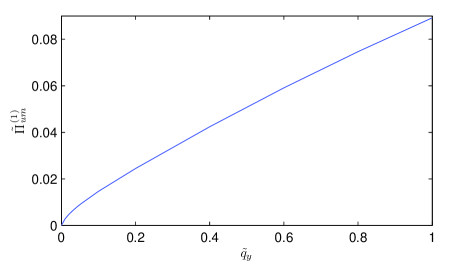
Figure 9: The dependence of $\tilde{\Pi}_{um}^{(1)}(0,\tilde{q}_{y},0)-\tilde{\Pi}_{um}^{(1)}(0,0,0)$ on $\tilde{q}_{y}$.

The integration over $U,X,Y$ has been done numerically. Just as we did in the calculation of the one-loop polarization operator, we subtract from $\tilde{\Pi}_{um}^{(1)}(0,\tilde{q}_{y},0)$ its value at zero momentum $\tilde{\Pi}_{um}^{(1)}(0,0,0)$ to make the integral infra-red convergent. The term we subtract only shift the position of the QCP and is not of interest to us. After the subtraction, the integration in (90) can be extended to an infinite range.

We plot $\tilde{\Pi}_{um}^{(1)}(0,\tilde{q}_{y},0)-\tilde{\Pi}_{um}^{(1)}(0,0,0)$ in FIG. 9. We see that numerically $\tilde{\Pi}_{um}^{(1)}(0,\tilde{q}_{y},0)-\tilde{\Pi}_{um}^{(1)}(0,0,0)$ is small even when ${\tilde{q}}_{y}=1$.

The $O(\lambda)$ correction to $\chi^{(0)}$, which we need for the calculation of the right prefactor for $T_{c}$, is related to $\tilde{\Pi}_{um}^{(1)}(0,\tilde{q}_{y},0)-\tilde{\Pi}_{um}^{(1)}(0,0,0)$ as

$$\chi^{(0)}\rightarrow\chi^{(0)}-\lambda\int_{-\infty}^{\infty}dz\frac{\tilde{\Pi}_{um}^{(1)}(0,z,0)-\tilde{\Pi}_{um}^{(1)}(0,0,0)}{\left(z^{2}+\sqrt{|z|/2}\right)^{2}},$$ (91)

Using the numerical results for $\tilde{\Pi}_{um}^{(1)}(0,\tilde{q}_{y},0)-\tilde{\Pi}_{um}^{(1)}(0,0,0)$, we found that the renormalization of $\chi^{(0)}$ by the vertex correction in the polarization operator is

$$\chi^{(0)}\rightarrow\chi^{(0)}(1-0.042\lambda),$$ (92)

We cited this result in Eq. (53) in the main text.

Appendix C Contribution to $T_{c}$ from Kohn-Luttinger diagrams at finite momentum cutoff

We found in the main text that Kohn-Luttinger diagrams renormalize the transition temperature $T_{c}$ to

$$T_{c}=T_{c3}\exp{B},$$ (93)

where $T_{c3}$, given by Eq. (54), is the transition temperature without Kohn-Luttinger contributions, and $B$ is the prefactor for $k_{y}$ term term in the integral equation

$$A(k_{y})+C(k_{y})=Bk_{y}(\chi^{(0)})^{2}.$$ (94)

where $A$ and $C$ are given by

$$A(k_{y}) =\int_{-\Lambda}^{\Lambda}dq_{y}\left[\frac{\chi^{(0)}(q_{y})}{\chi^{(0)}}\delta\Phi(k_{y}+q_{y})\right]-\delta\Phi(k_{y})$$

$$C(k_{y}) =\int_{-\Lambda}^{\Lambda}dq_{y}q_{y}\chi^{(1)}(k_{y},q_{y}),$$ (95)

and we remind that $\chi^{(0)}(q_{y})=1/(q^{2}_{y}+\sqrt{|q_{y}|/2})$, $\chi^{(0)}$ is the number ($=6.09$), and $\chi^{(1)}(k_{y},q_{y})$ accounts for the contributions from Kohn-Luttinger diagrams. We also used shorthand notations $\delta\Phi(k_{y})\equiv\delta\Phi(k_{x}=0,k_{y},\omega_{m}=0)$ and $\chi^{(1)}(k_{y},q_{y})\equiv\chi^{(1)}(k_{x}=0,k_{y},\omega_{m}=0;q_{x}=0,q_{y},\omega_{m}^{\prime}=0)$ and we explicitly restricted the momentum integration to $|q_{y}|<\Lambda$, where $\Lambda$ is the upper momentum cutoff for the low-energy theory.

To obtain $B$, we take the first and second derivatives of Eq. (94):

$$A^{\prime}(k_{y})+C^{\prime}(k_{y}) =B(\chi^{(0)})^{2},$$ (96)

$$A^{\prime\prime}(k_{y})+C^{\prime\prime}(k_{y}) =0.$$ (97)

Integrating Eq. (97) from its lower limit $-\Lambda$ to $k_{y}$, we find

$$A^{\prime}(k_{y})+C^{\prime}(k_{y}) =A^{\prime}(-\Lambda)+C^{\prime}(-\Lambda).$$ (98)

Hence

$$B(\chi^{(0)})^{2}=A^{\prime}(-\Lambda)+C^{\prime}(-\Lambda).$$ (99)

Now, let’s explicitly write down

$$A^{\prime}(-\Lambda)=\int_{-\Lambda}^{\Lambda}dq_{y}\frac{\chi^{(0)}(q_{y})}{\chi^{(0)}}\left[\delta\Phi^{\prime}(q_{y}-\Lambda)-\delta\Phi^{\prime}(-\Lambda)\right]$$ (100)

Typical values of $q_{y}$ are set by $\chi^{(0)}(q_{y})$ and are order $O(1)$. Because $\Lambda\gg 1$ by construction, $\delta\Phi^{\prime}(q_{y}-\Lambda)-\delta\Phi^{\prime}(-\Lambda)=O(1/\Lambda)$, i.e., $A^{\prime}(-\Lambda)$ is small and can be neglected. Then

$$B(\chi^{(0)})^{2}=C^{\prime}(-\Lambda)=\int_{-\Lambda}^{\Lambda}dq_{y}q_{y}\left.\frac{\partial\chi^{(1)}(k_{y},q_{y})}{\partial k_{y}}\right|_{k_{y}=-\Lambda}.$$ (101)

We now need the explicit expression for $\chi^{(1)}(k_{y},q_{y})$. Evaluating explicitly the three Kohn-Luttnerg contributions in FIG. 7, we obtain, for zero external frequency and $x$-component of momenta $\chi^{(1)}(k_{y},q_{y})=2\chi_{a}^{(1)}(k_{y},q_{y})+\chi_{b}^{(1)}(k_{y},q_{y})$, where

$$\chi_{a}^{(1)}(k_{y},q_{y};\lambda)$$

$$=-\frac{1}{8\pi^{2}}\int\frac{du~{}dx~{}dy}{iu-x-\lambda^{2}(k_{y}-y)^{2}}\frac{1}{iu+x-\lambda^{2}(q_{y}-y)^{2}}$$

$$\times\frac{1}{x^{2}+y^{2}+\sum_{a=\pm 1}\tilde{\Pi}_{a}^{(0)}(x,y,u)}\frac{1}{(k_{y}-q_{y})^{2}+\sqrt{|k_{y}-q_{y}|/2}}$$ (102)

and

$$\chi_{b}^{(1)}(k_{y},q_{y};\lambda)$$

$$=-\frac{3}{8\pi^{2}}\int\frac{du~{}dx~{}dy}{iu-x-\lambda^{2}(k_{y}+y)^{2}}\frac{1}{iu+x-\lambda^{2}(q_{y}-y)^{2}}$$

$$\times\frac{1}{x^{2}+y^{2}+\sum_{a=\pm 1}\tilde{\Pi}_{a}^{(0)}(x,y,u)}\frac{1}{x^{2}+(y+k_{y}-q_{y})^{2}+\sum_{a=\pm 1}\tilde{\Pi}_{a}^{(0)}(x,y+k_{y}-q_{y},u)}.$$ (103)

The difference in prefactors comes from different structures in Pauli matrices convolution and is trivial to verify. In these two integrals the ${\lambda^{2}}$ terms in the denominator, together with external momenta $k_{y}$ and $q_{y}$, serves as an infra-red cutoff.

One can easily make sure that the magnitude of $C^{\prime}(-\Lambda)$ depends on the value ${\lambda}^{2}\Lambda^{2}$. One can show that, if the momentum cutoff along the FS is of order $k_{F}$, ${\lambda^{2}}\Lambda^{2}\sim(W/\bar{g})^{2/3}\gg 1$, where $W$ is the fermionic bandwidth. In this case we find that $B(\chi^{(0)})^{2}=C^{\prime}(-\Lambda)\ll 1$. Then $B\ll 1$, and the renormalization due to Kohn-Luttinger-type diagrams are small.

If, however, the momentum cutoff $\Lambda$ is much smaller such that $\lambda\Lambda$ is actually a small number, the integral for $C^{\prime}(-\Lambda)$ in (101) contains $\log\frac{1}{\lambda\Lambda}$. Collecting the contributions from (102) and (103), we obtain at $\lambda\Lambda\ll 1$

$$C^{\prime}(-\Lambda) =\frac{10}{3}\left(\chi^{(0)}\right)^{2}\log\frac{1}{\lambda\Lambda}+O(1)$$ (104)

Using Eqs. (101) and (93), we find that $T_{c}$ in this case will be enhanced by a factor of $\exp B\sim\left({\lambda\Lambda}\right)^{-10/3}$.

References

• (1) S. Sachdev, “Quantum Phase Transitions”, Cambridge University Press (2011).
• (2) P. Coleman, A. J. Schofield Nature vol 433, 226-229 (2005).
• (3) Ar. Abanov, A.V. Chubukov, and J. Schmalian, Adv. Phys. 52, 119 (2003).
• (4) A.-M.S. Tremblay, a chapter in “Theoretical methods for Strongly Correlated Systems”, Edited by A. Avella and F. Mancini, Springer Verlag, (2011).
• (5) N.E. Bonesteel, I.A. McDonald, and C. Nayak, Phys. Rev. Lett. 77, 3009 (1996).
• (6) D. V. Khveshchenko and W. F. Shively, Phys. Rev. B 73, 115104 (2006); A. V. Chubukov and A. M. Tsvelik, Phys. Rev. B 76, 100509 (2007).
• (7) D. T. Son, Phys. Rev. D. 59, 094019 (1999); A. V. Chubukov, and J. Schmalian, Phys. Rev. B. 72, 174520 (2005); Eun-Gook Moon, A. V. Chubukov, J. Low. Temp. Phys. 161, 263 (2010).
• (8) P. A. Lee, Phys. Rev. Lett. 63, 680 (1989); J. Polchinski, Nucl. Phys. B 422, 617 (1994); C.J. Halboth and W. Metzner, Phys. Rev. Lett. 85, 5162 (2000); B. L. Altshuler, L. B. Ioffe, and A. J. Millis, Phys. Rev. B 50, 14048 (1994).
• (9) M. A. Metlitski and S Sachdev, Phys. Rev. B 82, 075127 (2010).
• (10) Y.-B. Kim, A. Furusaki, X.-G. Wen, and P. A. Lee, Phys. Rev. B 50, 17917 (1994); H.-Y. Kee and Y.-B. Kim, Phys. Rev. B 71, 184402 (2005); Z. Wang, W. Mao, and K. Bedell, Phys. Rev. Lett., 87, 257001 (2001). R. Roussev and A.J. Millis, Phys. Rev. B 63, 140504 (2001); A. V. Chubukov, A. M. Finkelstein, R. Haslinger, and D. K. Morr, Phys. Rev. Lett. 90, 077002 (2003).
• (11) A. J. Millis, S. Sachdev, and C. M. Varma, Phys. Rev. B 37, 4975 (1988)
• (12) Ar. Abanov, A. V. Chubukov, and A.M. Finkelstein, Europhys. Lett. 54, 488 (2001).
• (13) P. Monthoux, D. Pines, and G. G. Lonzarich, Nature 450, 1177, (2007); Shinya Nishiyama, K. Miyake, and C.M. Varma, arXiv:1302.2160.
• (14) M. A. Metlitski and S Sachdev, Phys. Rev. B 82, 075128 (2010).
• (15) K. B. Efetov, H. Meier, and C. Pépin, Nat. Phys. 9, 442 (2013).
• (16) E. Gull, A. J. Millis, Phys. Rev. B 86, 241106(R) (2012).
• (17) E. G. Moon, and S. Sachdev, Phys. Rev. B 80, 035117 (2009).
• (18) see e.g., G. M. Eliashberg, JETP 12, 1000 (1961); W. L. McMillan, Phys. Rev., 167, 331 (1968); J . Appel, Phys. Rev. Lett., 21, 1164 (1968); D. J. Scalapino, Superconductivity, 1, ed. R. D, Parks New York, 1969,p. 449; G Bergman and D. Rainer, Zs. Phys., 263, 59 (1973); P.B. Allen and R.C. Dynes, Phys. Rev. B 12, 905 (1975); R. Combescot, Phys. Rev. B 51, 11625 (1995) and references theren; F. Marsiglio and J.P. Carbotte, “Electron- Phonon Superconductivity”, in “The Physics of Conventional and Unconventional Superconductors”, edited by K.H. Bennemann and J.B. Ketterson, Springer-Verlag, 2006.
• (19) Y. Wang and A. V. Chubukov, Phys. Rev. Lett. 110, 127001 (2013).
• (20) D. J. Scalapino, E. Loh, Jr., and J. E. Hirsch, Phys. Rev. B 34, 8190 (1986); M. T. Beal-Monod, C. Bourbonnais, and V. J. Emery, Phys. Rev. B 34, 7716 (1986).
• (21) D. J. Scalapino, Rev. Mod. Phys. 84, 1383 (2012).
• (22) T. Moriya and K. Ueda, Rep. Prog. Phys. 66, 1299 (2003).
• (23) D. Manske, Theory of Unconventional Superconductors, Springer, Berlin (2004); M. Eschrig, Adv. in Physics 55, 47, (2006); T. Dahm et al., Nature Physics 5, 217 (2009). M.V.Sadovskii, Proc. I.E. Tamm seminar, pp 357-441, Scientific World, Moscow 2007; N. M. Plakida, “High-Temperature Cuprate Superconduc- tors”, Springer Series in Solid-State Sciences, Vol. 166, Springer-Verlag, Berlin, 2010.
• (24) P. Prelov¡sek and A. Ramisak, Phys. Rev. B, 72, 012510 (2005).
• (25) T. Das, R. S. Markiewicz and A. Bansil, Phys. Rev. B 74, 020506 (2006)
• (26) D. Manske, I. Eremin, and K. H. Bennemann, Phys. Rev. B 62, 13922 (2000).
• (27) B. Kyung, J.S. Landry, and A.-M.S. Tremblay, Phys. Rev. B 68, 174502 (2003).
• (28) T. Das, R. S. Markiewicz, and A. Bansil , Phys. Rev. B 81, 184515 (2010)
• (29) A.J. Millis, Phys. Rev. B 45, 13047 (1992).
• (30) D. F. Mross, J. McGreevy, H. Liu, and T. Senthil, Phys. Rev. B 82, 045121 (2010).
• (31) B.L. Altshuler, L.B. Ioffe, A.J. Millis, Phys. Rev. B 52, 5563 (1995).
• (32) B. Kyung, V. Hankevych, A.-M. Daré, and A.-M. S. Tremblay, Phys. Rev. Lett. 93, 147004 (2004).
• (33) A. Damascelli, Z. Hussain, and Z.X. Shen, Rev. Mod. Phys. 75, 473 (2003); N.P. Armitage, P. Fourier, and R.L. Greene, Rev. Mod. Phys., 82, 2421 (2010) and references therein.
• (34) A. J. Millis, A. Zimmers, R. P. S. M. Lobo, N. Bontemps, and C. C. Homes, Phys. Rev. B 72, 224517 (2005); A. Zimmers, J. M. Tomczak, R. P. S. M. Lobo, N. Bontemps, C. P. Hill, M. C. Barr, Y. Dagan, R. L. Greene, A. J. Millis and C. C. Homes, Europhys. Lett. 70, 225 (2005).
• (35) A. Koitzsch, G. Blumberg, A. Gozar, B. S. Dennis, P. Fournier, and R. L. Greene, Phys. Rev. B67, 184522 (2003).
• (36) L. Alff, Y. Krockenberger, B. Welter, M. Schonecke, R. Gross, D. Manske, M. Naito, Nature 422, 698 (2003).
• (37) E.M. Motoyama, G. Yu, I.M. Vishik, O.P. Vajk, P.K. Mang, and M. Greven, Nature 445, 186 (2007).
• (38) F. Onufrieva and P. Pfeuty, Phys. Rev. Lett. 92, 247003 (2004). See also R.S. Markiewicz, “Intrinsic Multiscale Structureand Dynamics in Complex Electronic Oxides”, World Scientific, Singapore (2003); Y. J. Wang, B. Barbiellini, H. Lin, T. Das, S. Basak, P. E. Mijnarends, S. Kaprzyk, R. S. Markiewicz, and A. Bansil, Phys. Rev. B 85, 224529 (2012).
• (39) P. Krotkov, A. V. Chubukov Phys. Rev. Lett. 96, 107002 (2006); Phys. Rev. B 74, 014509 (2006).
• (40) D. Dhokarh and A. V. Chubukov, Phys. Rev. B 83, 064518 (2011).
• (41) D. Bergeron, D. Chowdhury, M. Punk, S. Sachdev, and A.-M. S. Tremblay, Phys. Rev. B 86, 155123 (2012).
• (42) A. V. Chubukov and D. L. Maslov, Phys. Rev. B 86, 155136 (2012).
• (43) K. Jin, N. P. Butch, K. Kirshenbaum, J. Paglione, R. L. Greene, Nature, 476, 73 (2011); N. P. Butch, K. Jin, K. Kirshenbaum, R. L. Greene, J. Paglione, Proc. Natl. Acad. Sci. 109, 8440-8444 (2012). For similar studies of hole-doped cuprates see R. A. Cooper, Y. Wang, B. Vignolle, O. J. Lipscombe, S. M. Hayden, Y. Tanabe, T. Adachi, Y. Koike, M. Nohara, H. Takagi, Cyril Proust, and N. E. Hussey, Science 323, 603-607 (2009); L. Taillefer, Annu. Rev. Condens. Matter Phys. 1, 51-70 (2010).
• (44) L.P. Gorkov and T.K. Melik-Barkhudarov, Sov. Phys. JETP, 13, 1018 (1961). For more recent works see W.E. Brown, J.T. Liu, and H.-C. Ren, Phys. Rev. D 61, 114012 (2000); 62, 054013 (2000); 62, 054016 (2000); Q. Wang and D.H. Rischke, Phys. Rev. D 65, 054005 (2002); A.V. Chubukov and A. Sokol, Phys. Rev. B 49, 678 (1994); D. Efremov, M.S. Marienko, M.A. Baranov, and M. Yu. Kagan, JETP 90, 861 (2000).
• (45) W. Kohn, J.M. Luttinger, Phys. Rev. Lett. 15, 524 (1965); J.M. Luttinger, Phys. Rev.150, 202 (1966).
• (46) Y Onose, T. Taguchi, K. Ishizaka, and Y. Tokura, Phys. Rev. B 69, 024504 (2004).
• (47) N. P. Armitage et. al, Phys. Rev. B, 68, 064517 (2003).
• (48) Y. Dagan, M. M. Qazilbash, C. P. Hill, V. N. Kulkarni, and R. L. Greene, Phys. Rev. Lett. 92, 167001 (2004).
• (49) Ar. Abanov, A.V. Chubukov, and M. Norman, Phys. Rev. B 78, 220507 (2008).
• (50) H. Takagi, S. Uchida, and Y. Tokura, Phys. Rev. Lett. 62, 1197 (1989); Y. Tokura, H. Takagi, and S. Uchida, Nature (London) 337, 345 (1989).
• (51) M. M. Qazilbash, and A. Koitzsch, and B. S. Dennis, A. Gozar, Hamza Balci, C. A. Kendziora, and R. L. Greene, and G. Blumberg, Phys. Rev. B 72, 214510 (2005).
• (52) A. E. Karakozov, E.G. Maksimov, and S. A. Mashkov, Sov. Phys. JETP 41, 971 (1976).
• (53) W. Kessel, Z. fur Naturforschung A 29, 445 (1974); P Hertel, Z. fur Phys., 248, 272 (1971); B. T. Geilikman and N. F. Masharov, J. Low Temp. Phys., 6, 131 (1972);
• (54) O.V. Dolgov, I. I. Mazin, A. A. Golubov, S.Y. Savrasov, and E. G. Maksimov, Phys. Rev. Lett., 95, 257003 (2005); I.I. Mazin, Bull. Amer. Phys. Soc. 2006.
• (55) Strictly speaking, this decoupling is fully justified only when the theory is extended to $N\gg 1$ fermionic flavors because the fermionic self-energy, evaluated using $\chi(q,\Omega_{m})$ with Landau damping, does contain, along with the frequency depedence, also the dependence on the momenta along the FS, $k_{\parallel}$ The latter does affect the prefactor in $\Pi(Q,\Omega)=\gamma\Omega_{m}$. The relative change in $\gamma$ compated with the case when $\Sigma({\bf k},\omega_{m})=\Sigma(\omega_{m})$ is of order $1/N^{2}$ and is small at large $N$.
• (56) see e.g., Y. Tokura, S. Koshihara, T. Arima, H. Takagi, S. Ishibashi, T. Ido, and S. Uchida, Phys. Rev. B 41, 11657 (1990).
• (57) A. V. Chubukov and D. K. Morr, Phys. Rep. 288, 355 (1997); T. Sedrakyan and A.V. Chubukov, Phys. Rev. B 81, 174536 (2010).
• (58) T. Das, R. S. Markiewicz and A. Bansil, Phys. Rev. Lett. 98, 197004 (2007).
• (59) S. R. Hassan, B. Davoudi, B. Kyung, and A.-M.S. Tremblay Phys. Rev. B 77, 094501 (2008).
• (60) C. Weber, K. Haule, and G. Kotliar, Nature Phys. 6, 574-578 (2010); E. Gull, O. Parcollet, and A. J. Millis Phys. Rev. Lett. 110, 216405 (2013)