Cyclic motions in Dekel-Scotchmer Game Experiments

Abstract

TASP (Time Average Shapley Polygon, Benaīm, Hofbauer and Hopkins, Journal of Economic Theory, 2009), as a novel evolutionary dynamics model, predicts that a game could converge to cycles instead of fix points (Nash equilibria). To verify TASP theory, using the four strategy Dekel-Scotchmer games (Dekel and Scotchmer, Journal of Economic Theory, 1992), four experiments were conducted (Cason, Friedman and Hopkins, Journal of Economic Theory, 2010), in which, however, reported no evidence of cycles (Cason, Friedman and Hopkins, The Review of Economic Studies, 2013). We reanalysis the four experiment data by testing the stochastic averaging of angular momentum in period-by-period transitions of the social state. We find, the existence of persistent cycles in Dekel-Scotchmer game can be confirmed. On the cycles, the predictions from evolutionary models had been supported by the four experiments.
JEL classification: C72; C73; C92; D83

1 Introduction

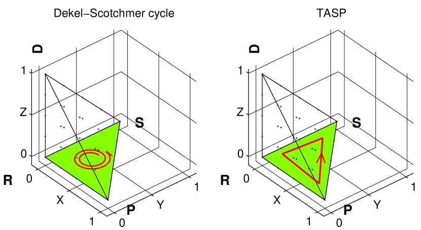
Figure 1: Cyclic trajectory and its angular momentum. (a) Ideal Dekel-Scotchmer cycle (refer to the Figure 1 in p396 in [1]) and (b) Time Average Shapley Polygon (TASP) (refer to the Figure 1 in p2313 in [2]) for unstable RPSD game. The frequencies of strategies $P$ and $S$ are on the horizontal axes and of strategy $D$ on the vertical axis. The red arrows indicate the accumulated angular momentum (vector) respects to the cycles.

While facing a game, the first step is to look for Nash equilibra (fixed points) [3], but in some condition, instead of fix points, a game could converge to cycles. As an example in evolutionary game theory catalog, recently, a dynamic theory — Time Average Shapley Polygon (TASP) theory [4] — is built giving a precise prediction about non-equilibrium play in games. To test TASP theory, four exemplified experiments of the Dekel-Scotchmer game [1], called also as Rock-Paper-Scissors-Dumb (RPSD) games [2], were conducted by Cason et al. [2]. The four experiments game were multi round repeated, set as discrete time (instead of continuous time as [5]), at the same time the matching protocol are randomly pair-wised which called as evolutionary protocol [6, 7]. In the four experiments, some evidences supporting TASP are found. But no cycle is reported in [2], which is emphasized by the authors in their recent literature [5]. In fact, this is the second time for the cycles in the Dekel-Scotchmer game was declined in experiments. This game had firstly been tested in experiments, no cycles was found which was also emphasised by the authors [6] (We go back this point in discussion, section 4). All these seems to suggest that there is no cycle in the four Dekel-Scotchmer game experiment.

As illustrated in Fig. 1, cycle should along $R$, $P$, $S$, $R$, $P$ … in the $RPS$ plane in the tetrahedronthe state space of the Dekel and Scotchmer game. Since the game was designed [1], not only TASP, variants evolutionary models has expected the cycle [4, 1, 8, 9, 10]. Empirically, as in biology system [11, 12], in experimental economics, evolutionary models have been supported extensively [13, 7, 14, 15, 16, 17]. Recently, in the discrete time protocol, the cycles have been constantly tested out [18, 19, 20, 21, 22, 23, 24, 25, 26, 27]. So, it is enigma that using the similar protocol in the four experiments, why does the RPS cycle not exist. The objective of this paper was to study whether or not cycle exists the four Dekel-Scotchmer game experiments.

The four experiments have a 2 $\times$ 2 design [2] shown in Table 1. The first design is the two game matrix. Both settings are Dekel-Scotchmer game constructed from the Rock-Paper-Scissors (RPS) game with the addition of a fourth strategy called Dumb ($D$). The payoff matrix can be presented as

$\begin{array}[]{lrrrr}&~{}~{}~{}~{}R&P&S&D\\ \end{array}$

$\begin{array}[]{l}R\\ P\\ S\\ D\\ \end{array}$ $\left[\begin{array}[]{rrrr}a&0&b&c\\ b&a&0&c\\ 0&b&a&c\\ d&d&d&0\end{array}\right]$.

For Unstable and Stable games, $[a~{}b~{}c~{}d]$ equals to [90 120 20 90] and [60 150 20 90], respectively. Both games have the same unique Nash-Dumb (the probability to choose Dumb is 1/2, shown as the redline in Fig. 2). The second design is two conversion rates of Experimental Francs (the entries in the game matrix) to US Dollars. In the High-pay (Low-pay) treatment, 100 EF = $5 ($2). In High-pay games, the monetary incentive for optimal strategy is stronger and less noise is expected. Mainly, the settings of the four game are summarized as shown in Table 1. While these games are identical in their equilibrium predictions, they differ quite substantially in terms of predicted learning behavior The stable games (game-2,3) would converge to the Nash equilibrium. At the same time, in the unstable game (game-0, 1), play will approach to a cycle (in RPS-plane, see green triangle in Fig. 3) in which there would be no weight placed on the strategy Dumb ($D$). So, the correction of TASP can be evaluated [2] by the average play of $D$ ($P_{D}$). The main result [2], as illustrated in $y$-axis in Fig 2, $P_{D}$ in game-1 leaves Nash Dumb the farthest and game-2 the closest. These meet TASP theory well.

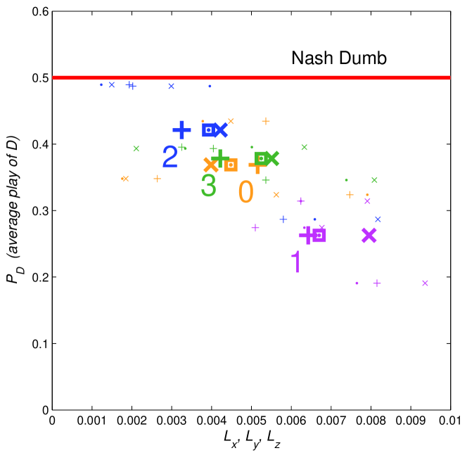
Figure 2: The relation between observed average angular momentum ($\bar{L}_{x},\bar{L}_{y},\bar{L}_{z}$) and observed average play of $D$ ($P_{D}$, see also the Table 1 in [2]). Observed ($\bar{L}_{x},\bar{L}_{y},\bar{L}_{z}$) can be obtained from $k$=1 rows in Table 5. Red line is Nash equilibrium Dumb ($D$-play). Color [yellow, purple, blue, green] presents game-[0,1,2,3], respectively. Symbol $(\square,\times,+)$ represents $(\bar{L}_{x},\bar{L}_{y},\bar{L}_{z})$ respectively. Enlarged symbols are the averages by games and smaller by sessions.

Cycles are also expected by TASP theory (Fig.1) in these four games. The theoretical arguments of the fictitious learning model have been well analyzed [2] —— For the game treatment, as the basic argument (p.2312 in [2]), in the stable game there would be convergence to the Nash equilibrium. In the unstable game, however, there will be divergence from equilibrium and play will approach a cycle in which no weight is placed on the strategy Dumb (D). For the payoff treatment, high-pay has the same effect as an increase in the noise parameter (p.2317 in [2]) —— Accordingly, the quantitative expectation is that the more deviation from equilibrium, the more cyclic motion will be, which forms the second testable point following presented by Table 1. For the objective of this paper, the expectation on cycle could be decomposed into three testable hypothesis:

(1) Cycles exist only along $R,P,S,R$,… direction shown in Fig. 3 and Table 5. Explanation for this testable points see section 2.4. The results, see section 3.1, support this point.

(2) Cycles’ strength depends on games, shown in Table 1, in which game-1 is the largest. Results, see section 3.2, support this point.

(3) Cycles’ persistence depends on games, in which game-1 performs the best. Results, see section 3.3, support this point.

These three hypothesis are tested in this paper. Using angular momentum (an observation of rotation in classical physics), in the period-by-period transitions (PPT) of social state in the four experiments [2], we test the cycles and find that all the three theoretical arguments are supported in significant. we hope our observation can provides an exemplified evidence of the existence of Dekel-Scotchmer cycles.

Table 1: The four games (treatments)

game i.d.	Low pay		High pay
Unstable	0	$\leftarrow$	1
	$\downarrow$		$\downarrow$
Stable	2	$\leftarrow$	3

Each game has 3 repeated sessions with 12 subjects in each session. Game in each session is about 80 times repeated. Matching protocol is randomly pairwise. On cycle expected by RPS-CH, $a\rightarrow b$ presents the strength in game-$a$ larger than that in game-$b$ ($\bar{L}_{a}>\bar{L}_{b}$). The related empirical results are shown in Table 5.

2 Methods

2.1 State space settings

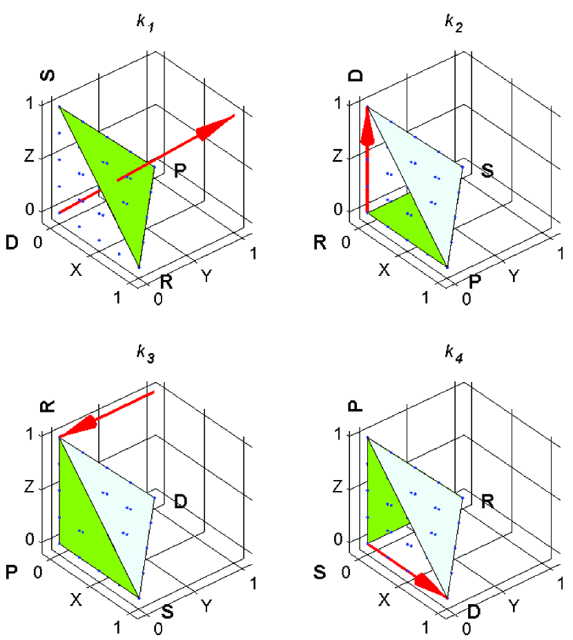
Figure 3: Social state space of the RPSD game in 3D representation. Each social state is represented by a (blue) dot. Each $k_{1},k_{2},k_{3},k_{4}$ setting, see the $x-y-z;O$-column in Table 5, is illustrate as a sub-figure. The green triangle is the RPS-plane. The red arrow indicating $L$-direction if the net notations are along $R\!\rightarrow\!P\!\rightarrow\!S\!\rightarrow\!R$ (expected by TASP theory see the ($L_{x},L_{y},L_{z}$)-columns in Table 5). For example, in $k_{2}$ setting, the red arrow is (0,0,1) which means ($L_{x}=0,L_{y}=0,L_{z}>0$) are expected.

There are four pure strategies in the game, therefore we use a four dimensional (4D) vector $(x,y,z,u)$ to denote a generic social state of the population, where $x$, $y$, $z$ and $u$ are the fractions of players using strategy $R$, $P$ $S$ and $D$, respectively [19, 16]. The fraction must be one element in ($0,1/N,2/N...,1$) set in an $N$-players game. There are 4 pure social states which can be denoted as $W_{i}$ ($i\!\in\!\{R,P,S,D\}$). At the same time, the sum of the fractions is 1 ($x+y+z+u$=1), the 4D space is constrained. Hence, it can be projected into a 3D space.

By the permuting $D,R,P,S$ at $O$=(0,0,0) and other three at $x,y,z$-axis respectively, there could have four ways (denoted as $k_{1},k_{2},k_{3},k_{4}$) to realize the projections. See column-($x,y,z;O$) in Table 5 for the assignments. The four 3D spaces can be presented graphically as a trirectangular tetrahedron lattice as illustrated in Fig. 3.

2.2 Period-by-period transition (PPT)

In such lattice space, generically speaking, the observed social state depends on time. From one period ($t$) to its next period ($t+1$), one social state transition from $x(t)$ to $x(t+1)$ , called as one period-by-period transition (PPT), can be observed. Each PPT is a 3D vector in the lattice space. Successive PPT vectors form an evolutionary trajectory in 3D. For example, in a 80 rounds experimental sessions, an evolutionary trajectory of 80 nodes in which there are 79 PPT can be obtained.

2.3 Angular momentum in PPT

For simplicity we consider first a particle (with mass $m$=1) moving with respect to a specific reference point (denoted as $o$). Consider one PPT, from $x(t)$ to $x(t+1)$, the instantaneous angular momentum vector $L(t)$ can be expressed as [21]

$$L(t) = \left[x(t)-o\right]\times\left[x(t\!+\!1)-o\right],$$ (1)

in which symbol $\times$ means cross product of the two vectors. So, $L(t)$ has a magnitude equal to the area of the parallelogram with edges $\left[x(t)-o\right]$ and $\left[x(t\!+\!1)-o\right]$, has the attitude of the plane spanned by $\left[x(t)-o\right]$ and $\left[x(t\!+\!1)-o\right]$, and has orientation being the sense of the rotation that would align $\left[x(t)-o\right]$ with $\left[x(t\!+\!1)-o\right]$. It does not have a definite location or position [28]. No lose of the generality, the random mixed (1,1,1,1)/4 is used as the reference point to report the following results.

This measurement can be interpreted as following. In equilibrium, in long run, the time average of $L$ (denoted as $\bar{L}$) is 0, because of the detailed balance in PPT [18, 29]. In non-equilibrium, $\bar{L}$ should be significantly different from zero which provides combinative cycles’ information (strength and direction of rotation) of the ”tumbling cycles”. This way is to proceed from the microscopic level motions to the macro level observation by stochastic averaging [30, 31, 32, 33] over PPT.

In our studies case, there are three components ($L_{x},L_{y},L_{z}$) of an $L$. Each component describes the rotation along its own directions respectively. So, each PPT can provide one sample in each of the three directions respectively. In sufficient samples, if a component $\bar{L}_{w}$ ($w\in\{x,y,z\}$) deviates from 0 with the statistic significance, cycles exist in the direction.

As mentioned above, to our study case, we have four coordination settings ($k_{1},k_{2},k_{3},k_{4}$). For different settings, the observable $\bar{L}_{w}$ ($w\in\{x,y,z\}$) of a experimental trajectory should be different.

2.4 Construct the testable points table

The testable points tables are Table 5 and Table 5. Lets see an example for constructing the testable points tables.

If the $R$, $P$ and $S$ are at (0,0,0), (1,0,0) and (0,1,0) respectively (setting $k_{2}$, see Table 5), in long run, the only $\bar{L}$ components deviating from 0 with the statistic significance should be $L_{z}$. Because, TASP predicts that cycles exist only in the X-Y plane along R,P,S,R…. According to $L$ definition in Eq 1, observed $L$ should have only the component on the $Z$ direction upwards. This can be shown in $k_{2}$ setting in Fig. 3 and $k$=2 condition in Table 5. In same way, for each of the ($k_{1},k_{2},k_{3},k_{4}$) setting, expected observation of $L$ can be represented as red arrows in Fig. 3. At the same time, in matrix form, testable expectations on these four settings are shown in Table 5 too.

In summary, for the four games and four coordination setting, RPS-CH falls into 48 (3 $L$-components $\times$ 4 coordination settings $\times$ 4 games) testable points listed in the right-most three columns in Table 5. Respectively, present the evolutionary trajectory in four coordination settings, then we measure the $L$ using Eq. 1 for the four games in in the experiments. Then, we can compare the actual motion with the three hypothesis above.

Table 2: Testable TASP hypothesis on $\bar{L}_{x},\bar{L}_{y},\bar{L}_{z}$

Setting ($k$)	$x$-$y$-$z$; $O$	$\bar{L}_{x}$	$\bar{L}_{y}$	$\bar{L}_{z}$
1	$R$-$P$-$S$; $D$	+	+	+
2	$P$-$S$-$D$; $R$	$\bigcirc$	$\bigcirc$	+
3	$S$-$D$-$R$; $P$	$\bigcirc$	–	$\bigcirc$
4	$D$-$R$-$P$; $S$	+	$\bigcirc$	$\bigcirc$

Setting three of the four pure strategies along column $x$-$y$-$z$ [$e_{x}=(1,0,0)$, $e_{y}=(0,0,1)$, $e_{z}=(0,0,1)$], meanwhile, $O$ state assigned at (0,0,0). Testable hypotheses (PRS-CH) are in last 3 columns in which ’+’ (’–’) or $\bigcirc$ means the $L_{w}$ should along (oppose to) $w$-axis direction or not deviating from 0.

Table 3: Experimental ($\bar{L}_{x},\bar{L}_{y},\bar{L}_{z}$)$\times 10^{-3}$ in four setting

$k$	game	$\bar{L}_{x}$	$\bar{L}_{y}$	$\bar{L}_{z}$	$p_{x}$	$p_{y}$	$p_{z}$
1	0	4.5	4.0	5.2	+∗∗∗	+∗∗∗	+∗∗∗
1	1	6.7	8.0	6.4	+∗∗∗	+∗∗∗	+∗∗∗
1	2	3.9	4.2	3.3	+∗∗∗	+∗∗∗	+∗∗
1	3	5.2	5.5	4.2	+∗∗∗	+∗∗∗	+∗∗∗
2	0	0.5	-0.7	4.5	$\bigcirc$	$\bigcirc$	+∗∗∗
2	1	-1.3	0.3	6.7	$\bigcirc$	$\bigcirc$	+∗∗∗
2	2	-0.3	0.7	3.9	$\bigcirc$	$\bigcirc$	+∗∗∗
2	3	-0.3	1.0	5.2	$\bigcirc$	$\bigcirc$	+∗∗∗
3	0	1.2	-4.0	0.5	$\bigcirc$	–∗∗∗	$\bigcirc$
3	1	-1.5	-8.0	-1.3	$\bigcirc$	–∗∗∗	$\bigcirc$
3	2	-1.0	-4.2	-0.3	$\bigcirc$	–∗∗∗	$\bigcirc$
3	3	-1.3	-5.5	-0.3	$\bigcirc$	–∗∗∗	$\bigcirc$
4	0	5.2	0.7	1.2	+∗∗∗	$\bigcirc$	$\bigcirc$
4	1	6.4	-0.3	-1.5	+∗∗∗	$\bigcirc$	$\bigcirc$
4	2	3.3	-0.7	-1.0	+∗∗	$\bigcirc$	$\bigcirc$
4	3	4.2	-1.0	-1.3	+∗∗∗	$\bigcirc$	$\bigcirc$

Superscript [^(.), ^(∗), ^(∗∗), ^(∗∗∗)] represents $p$ less than [0.2, 0.1, 0.05, 0.01]. $p_{w}$-values coming from one-sample ttest with null hypothesis that the population mean $\bar{L}_{w}$ is equal to 0. The sample sizes for each test point are the total number of PPT and are [237, 217, 237, 237] for game-[0,1,2,3], respectively.

Table 4: $|L|$ and cross game comparison for $(L_{x},L_{y},L_{z})$ $\times 10^{-3}$

game	$|L|$	1	2	3
0	7.9	–${}^{\circ},$–${}^{**},$–∗	–,+,–	–,–,+
1	12.2		+∘,+∗∗,+∗∗	+,+,+∗
2	6.6			–,–,–
3	8.7

Compare (Wilcoxon rank sum) cycle strength of the game in row to the game in column. For example, the symbol (–^∘) in 3rd column means $L_{x}$ in game-0 is smaller than game-1 (at $p<0.2$). Definition of the superscript is as Table 5.

Table 5: Time dependence of $\bar{L}^{(1,1,1)}$ $\times 10^{-3}$

game	$\bar{L}_{1,40}^{(1,1,1)}$	$\bar{L}_{41,80}^{(1,1,1)}$	$\Delta\bar{L}^{(1,1,1)}$	Samples
0	7.5	1.7	-5.8∗∗∗	(351, 351)
1	7.1	6.9	-0.2	(351, 321)
2	4.9	2.7	-2.2	(351, 351)
3	5.1	4.3	-0.8	(351, 351)

$(a,b)$ in Samples column indicates the samples from (1st,2nd)-half periods in the game sessions. Statistic uses ttest with $\Delta\bar{L}$=0

3 Results

3.1 Cycle existence and direction

Result: Cycles exist and only exist paralleling RPS-plane in all of the 4 game experiments. Cyclic evolutions are along $RPSR$… in all of the 4 game experiments.
Support material: Statistics results of ($L_{x},L_{y},L_{z}$), from 4 settings and games respectively, are shown in Table 5. In $k_{1}$ setting, the full D strategy is settle at (0,0,0). All the three components ($L_{x},L_{y},L_{z}$) $>$ 0 significant ($p<0.05$) for all of the 4 games. In $k_{2}$ setting, only $L_{z}>0$ is statistically significant $(p<0.05)$. A straightforward interpretation is that cycle exists and only exist in RPS-plane too. This result is supported by $k_{3}$ setting and $k_{4}$ setting. Comparing the theoretical expectations (Table 5) and empirical results (5), RPS-CH is supported at all of the 48 testable points.

The direction of existed cycles can be distinguished by taking the signal of ($L_{x},L_{y},L_{z}$) into account. Empirical signal (+ or – in Table 5) of ($L_{x},L_{y},L_{z}$), comparing with RPS-CH signal (+ or – in Table 5) by the $k$-settings and games respectively, one can find that RPS-CH is supported excellently at all of the 48 testable points too.

3.2 Cycle strength

Result: Strength of cyclic motion in game-1 (unstable and High-pay) is the largest. Strength of cycles is negatively dependent on $P_{D}$ (average play of Dumb).
Support material: The rotation strength of cycles can be quantified by the vector mode $|\bar{L}|$ $\!\equiv$ $\!(\bar{L}_{x}^{2}+\bar{L}_{y}^{2}+\bar{L}_{z}^{2})^{1/2}$. The game-1 has the largest rotation strength $|L|$ shown in the 2nd-column of Table 5. This result is also supported by the statistical test (Wilcoxon rank sum) by pair games comparison. In Table 5, over the 4 game, the strength orders can be compared with the arrows in Table 1. All the results meet RPS-CH [2] well.

Strength of cycles is negatively dependent on $P_{D}$ (average play of Dumb). At the same time, the result in Fig. 2 has to be explained —— Strength of cycles is negatively dependent on $P_{D}$ (average play of Dumb). This finding is statistically significant.

3.3 Cycle persistence

Result: Persistence of cycle in game-1 performs best. Except game-0, persistence of cycle can not be rejected by data.
Support material: One way to test the persistence of cycles is to compare $L$ samples in early and latter periods. In session level, the hypothesis ($L_{1,40}=L_{41,80}$) can not be rejected in general.

At game level to test the persistence, we can project $(L_{x},L_{y},L_{z})$ into (1,1,1)-vector in $k_{1}$ setting to build a combinative scale $L^{(1,1,1)}$. For $L^{(1,1,1)}_{1,40}$ and $L^{(1,1,1)}_{41,80}$ comparison, both have 351 samples, and results are shown in Table 5. One unexpected result is: in two low-pay treatment, $L^{(1,1,1)}$ in game-0 declines significantly and more strongly than that in game-2. Nevertheless, in the four treatments, cycle persistence in game-1 has the best performance, which meets TASP theory again.

4 Discussion

In the four exemplified experiments [2], firstly in this paper, the Dekel-Scotchmer cycles are reported. We looked and we see behavior with many of the properties the theorists [4, 1, 8, 9] told us that we would see. To the best of our knowledge, no only in Dekel-Scotchmer game, no cycle has been reported in any four strategy games before. These observed cycles, together with the cycles obtained in recent experiments [18, 19, 5], we wish, could provide a novel way to merger the expected and the actual motions.

In experiments, cycle, as the typical non-equilibrium phenomena, have been long sought but the necessary condition for its existence is unclear [16, 5, 18]. In this view, current paper could server as the third exemplified evidence between the two condition (the continuous time and full information environments [5] and the discrete time and only local information environments [18]). In the experiment investigated here, the time is discrete but the information is full. Nevertheless, the necessary conditions for cycle existence is still an open question.

In closed related literatures, as mentioned [5, 16], experimental work is surprisingly sparse. But one result, which is straightly contrasty to our results reported here, has to be reminded. Before [2], a series of RPSD games had been tested experimentally in 1999 by Von Huyck $et.al.$ [6]. One remarkable result is that: The subjects don’t exhibit the kind of correlated behavior predicted by the dynamic (p139 in [6]). Then, a conclusion was emphasized: A lesson from the experiment is that one should discount models that predict deterministic cycles (p148 in [6]). On the contrary, referring to the cycles observed from [5] data, we suggest that their results on the cycle in their data [6] are worth of being rechecked. Using cycle in Dekel-Scotchmer game as the exemplified calibration, we suggest, there has many cycles has been existed in existed experiment data.

For further investigations on the cycles of social motion, between laboratory experiments and evolutionary game theory, one central question is still: Whether the actual motions coincide with the expected motions and vise versa? As illustrated in [18, 5] the evolutionary trajectory can be calculated analytically or numerically based on a evolutionary model, so cyclic behaviors can be predicted theoretically. Together with stationary observations of a game (e.g., mean observations [36] and distribution in strategy space [19, 16]), observations of cycles (e.g. $L$ in this paper, frequency of cycle [18] and CRI [5]) can server as a set of calibrations to constraint game models.

References

- [1] E. Dekel, S. Scotchmer, On the evolution of optimizing behavior, Journal of Economic Theory 57 (2) (1992) 392–406.
- [2] T. N. Cason, D. Friedman, E. Hopkins, Testing the tasp: An experimental investigation of learning in games with unstable equilibria, Journal of Economic Theory 145 (6) (2010) 2309–2331.
- [3] J. F. Nash, Equilibrium points in n-person games, Proceedings of the national academy of sciences 36 (1) (1950) 48–49.
- [4] M. Benaīm, J. Hofbauer, E. Hopkins, Learning in games with unstable equilibria, Journal of Economic Theory 144 (4) (2009) 1694–1709.
- [5] T. N. Cason, D. Friedman, E. Hopkins, Cycles and instability in a rock-paper-scissors population game: a continuous time experiment, Review of Economic Studies 81 (2014) Forthcoming.
- [6] J. Van Huyck, F. Rankin, R. Battalio, What does it take to eliminate the use of a strategy strictly dominated by a mixture?, Experimental economics 2 (2) (1999) 129–150.
- [7] L. Samuelson, Evolution and game theory, The Journal of Economic Perspectives 16 (2) (2002) 47–66.
- [8] J. Weibull, Evolutionary game theory, The MIT Press, 1997.
- [9] W. Sandholm, Population games and evolutionary dynamics, The MIT Press, 2011.
- [10] C. Hauert, S. De Monte, J. Hofbauer, K. Sigmund, Volunteering as red queen mechanism for cooperation in public goods games, Science 296 (5570) (2002) 1129–1132.
- [11] B. Sinervo, C. Lively, The rock-paper-scissors game and the evolution of alternative male strategies, Nature 380 (6571) (1996) 240–243.
- [12] B. Kirkup, M. Riley, Antibiotic-mediated antagonism leads to a bacterial game of rock-paper-scissors in vivo, Nature 428 (6981) (2004) 412–414.
- [13] C. Plott, V. Smith, Handbook of experimental economics results, North-Holland, 2008.
- [14] D. Friedman, Equilibrium in evolutionary games: Some experimental results, The Economic Journal 106 (434) (1996) 1–25.
- [15] J. Van Huyck, Emergent conventions in evolutionary games, Handbook of Experimental Economics Results 1 (2008) 520–530.
- [16] M. Hoffman, S. Suetens, M. Nowak, U. Gneezy, An experimental test of nash equilibrium versus evolutionary stability (2012)., Nature Comm., submit.
- [17] S. K. Berninghaus, K.-M. Ehrhart, The power of ess: An experimental study, Journal of Evolutionary Economics 13 (2) (2003) 161–181.
- [18] B. Xu, H.-J. Zhou, Z. Wang, Cycle frequency in standard rock cpaper cscissors games: Evidence from experimental economics, Physica A: Statistical Mechanics and its Applications (0).
- [19] B. Xu, Z. Wang, Evolutionary Dynamical Pattern of ”Coyness and Philandering”: Evidence from Experimental Economics, Vol. VIII, p1313-1326, NECSI Knowledge Press, ISBN 978-0-9656328-4-3., 2011.
- [20] B. Xu, Z. Wang, Bertrand-edgeworth-shapley cycle in a game, SSRN eLibrary, 2010 International Workshop on Experimental Economics and Finance Program, Xiamen, December 15-16.
- [21] Z. Wang, B. Xu, Evolutionary rotation in switching incentive zero-sum games, arXiv preprint arXiv:1203.2591.
- [22] B. Xu, Cycles of strategies and changes of distribution in laboratory public goods games: An experimental investigation, ESA International Conference, 2013 ESA World Meetings in Zurich Accepted.
- [23] B. Xu, H. Zhou, Z. Wang, Asymmetry spectrum of cycle amplitude in rock-paper-scissor game of experimental economics, ESA International conference 2013, http://dx.doi.org/10.2139/ssrn.2085459.
- [24] B. Xu, Z. Wang, Social transition spectrum in constant sum 2x2 games with human subjects, SSRN eLibrary, Social Transition Spectrum in Constant Sum 2x2 Games with Human Subjects, http://dx.doi.org/10.2139/ssrn.1910045.
- [25] Z. Wang, B. Xu, Spontaneous time symmetry breaking in system with mixed strategy nash equilibrium: Evidences in experimental economics data, Bulletin of the American Physical Society 56 (2011).
- [26] B. Xu, Z. Wang, Test maxent in social strategy transitions with experimental two-person constant sum games, Results in Physics 2 (0) (2012) 127–134.
- [27] B. Xu, S. Wang, Z. Wang, Periodic frequencies of the cycles in 22 games, arXiv preprint arXiv:1208.6469.
- [28] D. Hestenes, New foundations for classical mechanics, Springer, 1999.
- [29] H. Young, Stochastic Adaptive Dynamics, New Palgrave Dictionary of Economics, revised edition, L. Blume and S. Durlauf, eds. Zanella, G.(2007), Discrete Choice with Social Interactions and Endogenous Membership, Journal of the European Economic Association 5 (2008) 122–153.
- [30] M. L. Deng, W. Q. Zhu, Stationary motion of active brownian particles, Physical Review E 69 (4) (2004) 046105.
- [31] W. Q. Zhu, M. L. Deng, Stationary swarming motion of active brownian particles in parabolic external potential, Physica A: Statistical Mechanics and its Applications 354 (2005) 127–142.
- [32] M. Deng, W. Zhu, Some applications of stochastic averaging method for quasi hamiltonian systems in physics, Science in China Series G: Physics, Mechanics and Astronomy 52 (8) (2009) 1213–1222.
- [33] G. Cai, Y. Lin, Stochastic analysis of time-delayed ecosystems, Physical Review E 76 (4) (2007) 041913.
- [34] J. Hofbauer, K. Sigmund, Evolutionary game dynamics, Bulletin of the American Mathematical Society 40 (4) (2003) 479.
- [35] C. Camerer, R. S. Foundation, Behavioral game theory: Experiments in strategic interaction, Vol. 9, Princeton University Press Princeton, NJ, 2003.
- [36] R. Selten, T. Chmura, Stationary concepts for experimental 2x2-games, The American Economic Review 98 (2008) 938–966.