Probing Vector Mesons in Deuteron Break-up Reactions

Abstract

We study vector meson photoproduction from the deuteron at high momentum transfer, accompanied by break-up of the deuteron into a proton and neutron. The large $-t$ involved allows one of the nucleons to be identified as struck, and the other as a spectator to the $\gamma N\rightarrow VN$ subprocess. Corrections to the plane wave impulse approximation involve final state interactions (FSIs) between the struck nucleon or the vector meson, either of which is energetic, with the slow spectator nucleon. In this regime, the eikonal approximation is valid, so is employed to calculate the cross-section for the reaction. Due to the high-energy nature of the FSIs, the maxima of the rescatterings are located at nearly transverse directions of the fast hadrons. This results in two peaks in the angular distribution of the spectator nucleon, each corresponding to either the $V$-$N$ or the $p$-$n$ rescattering. The $V$-$N$ peak provides a new means of probing the $V$-$N$ interaction. This is checked for near-threshold $\phi$ and $J/\Psi$ photoproduction reactions which demonstrate that the $V$-$N$ peak can be used to extract the largely unknown amplitudes of $\phi$-$N$ and $J/\Psi$-$N$ interactions.

Two additional phenomena are observed when extending the calculation of $J/\Psi$ photoproduction to the sub-threshold and high-energy domains. In the first case we observe overall suppression of FSI effects due to a restricted phase space for sub-threshold production in the rescattering amplitude. In the second, we observe cancellation of the $V$-$N$ rescattering amplitudes for vector mesons produced off of different nucleons in the deuteron.

I Introduction

Photoduction of vector mesons from nuclei with subsequent rescattering is the main approach in extracting the cross-sections of $V$-$N$ interactions that does not require the assumption of vector meson dominanceBauer et al. . To enhance the measured cross-sections, experiments have been carried out on medium to heavy nuclei, where the extraction of the $V$-$N$ scattering amplitude is based on the Glauber theory of multiple hadronic interactionsGlauber and Matthiae (1970). In several instances a deuteron target has been used, as it provides higher theoretical accuracy in the extraction of the $VN\rightarrow VN$ amplitudeBauer et al. . In the case of the deuteron target, one method is to study the coherent photoproduction at large $-t\geq 0.8~{}\mathrm{GeV}^{2}$Anderson et al. (1971); Frankfurt et al. (1997a); Rogers et al. (2006); Mibe et al. (2007), for which the $\gamma d\rightarrow Vd^{\prime}$ cross-section is primarily due to rescattering of the vector meson (first produced on a struck nucleon) off the spectator nucleon. This property has been used for probing both $\rho$-$N$Anderson et al. (1971); Frankfurt et al. (1997a) and $\phi$-$N$Mibe et al. (2007); Rogers et al. (2006) cross-sections. In these studies, calculations involving the elastic $V$-$N$ scattering amplitude are fit to experimental data to extract the total $V$-$N$ cross-section, the slope factor $B_{VN}$, and the ratio of the real and imaginary parts of the amplitude, $\alpha_{VN}$. However, this procedure has had limited success, since these parameters cannot be unambiguously disentangled by just the measurement of cross-sections. This situation can be improved by considering polarization observables of the coherent reactionFrankfurt et al. (1997a), but the experimental realization of polarization processes is more difficult.

In this work we suggest a new approach for measuring $V$-$N$ scattering cross section by considering vector meson photoproduction from the deuteron with subsequent break-up of the deuteron into a proton and neutron. We focus on kinematics with a large momentum transfer, for which the fast, “struck” nucleon can be unambiguously identified apart from the slow, “recoil” nucleon which is a spectator to the $\gamma N\rightarrow VN$ subprocess in the plane wave impulse approximation (PWIA). In this case, the final state interactions are characterized by a rescattering of either of the fast outgoing hadrons—the vector meson or the struck nucleon—with the spectator nucleon. By selecting the momentum and the direction of the spectator nucleon, one can increase the sensitivity of the reaction to small angle $V$-$N$ scattering, thereby probing the parameters of the $VN\rightarrow VN$ amplitude.

In addition to allowing identification of the struck and spectator nucleons, the large $-t$ establishes the applicability of the eikonal approximation to the hadronic rescatterings. In particular, we use the generalized eikonal approximation (GEA)Frankfurt et al. (1995a, 1997b); Sargsian (2001); Ciofi degli Atti and Kaptari (2005), which was developed to account for the finite target and recoil nucleon momenta neglected in the conventional Glauber approximation. GEA has been successfully applied to high energy electrodisintegration of the deuteronSargsian (2010), semi-inclusive deep inelastic scatteringCosyn and Sargsian (2011), and coherent photoproduction of $\rho$Frankfurt et al. (1997a) and $\phi$Rogers et al. (2006) mesons from the deuteron.

The most relevant of these to this paper is deuteron electrodisintegration, i.e. $ed\rightarrow e^{\prime}pn$, in which one of the nucleons is struck and the other is a spectator in PWIA. In this case the eikonal approximation predicts a clear $p$-$n$ rescattering peak when the differential cross-section is plotted against the spectator angle for spectator momenta larger than $400~{}\mathrm{GeV/c}$. This feature was experimentally confirmed in high momentum transfer deuteron break-up reactionsEgiyan et al. (2007); Boeglin et al. (2011).

In the reaction considered in this work, we see a new phenomenon, in which the presence of two energetic hadrons to rescatter from the slow spectator nucleon gives the possibility of observing two peaks, one associated with the $V$-$N$ and the other with the $p$-$n$ rescattering. One of our goals is to investigate whether the $V$-$N$ peak can be used to study the properties of the $V$-$N$ interaction amplitudes.

The article is organized as follows: In section II we consider the kinematics of the reaction and justify the application of the generalized eikonal approximation. In section III we calculate the amplitude for the reaction within the virtual nucleon approximation, in which the rescatterings are calculated based on GEA. In section IV we present numerical estimates for the break-up reaction, with photoproduction of $\phi(1020)$ and of $J/\Psi$. The appendix provides details of the calculation of the double rescattering amplitude.

II Reaction, kinematics and validity of eikonal approximation

We study large momentum transfer ($-t\geq 1~{}\mathrm{GeV}^{2}$) photoproduction from the deuteron accompanied by deuteron break-up:

$$\gamma+d\rightarrow V+p+n.$$ (1)

Our main goal is to investigate the feasibility of using this reaction to study the amplitude of $V$-$N$ scattering. This goal can be achieved only if it is possible to unambiguously isolate and reliably calculate the contribution of $V$-$N$ rescattering to the total cross-section to this reaction.

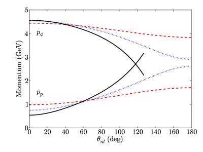
Figure 1: (Color online) Dependence of the momenta of struck nucleon and $\phi$ meson on the momentum and direction of the recoil nucleon, at $q_{0}=5~{}\mathrm{GeV}$ and $t=-1.2~{}\mathrm{GeV}^{2}$, for the reaction (1). The dashed (red), dotted (blue), and solid (black) curves correspond respectively to recoil momenta of $200$, $400$, and $600~{}\mathrm{MeV}$. The angle is defined with respect to the momentum transfer $\mathbf{l}$ defined in Eq. (2).

The experience of recent yearsSargsian (2010); Frankfurt et al. (1997a); Jeschonnek and Van Orden (2008); Ciofi degli Atti and Kaptari (2005); Ciofi degli Atti et al. (2001); Laget (2005); Mibe et al. (2007); Egiyan et al. (2007); Boeglin et al. (2011) demonstrates that such an isolation can be achieved in the eikonal regime, where the momenta of the rescattered fast hadrons are on the order of a GeV/c and above. The main advantage of the eikonal approximation is that the part of the $\gamma d\rightarrow Vpn$ amplitude corresponding to the pole values of the intermediate hadronic propagators is expressed through the on-shell hadronic rescattering amplitudes, which can be related to the experimental values of the total $V$-$N$ and $p$-$n$ cross-sections. The contribution from the principal value parts is expressed through half-off-shell hadronic amplitudes. In situations where the latter contributions are small, the eikonal regime provides the possibility of extracting on-mass-shell amplitudes of $V$-$N$ and $p$-$n$ elastic scattering in kinematics dominated by final state interactions.

To establish the eikonal regime for the reaction (1), we concentrate on kinematics where the subprocess $\gamma N\rightarrow VN$ has a large momentum transfer, and where just one of the nucleons emerges with a momentum $\gtrsim 1~{}\mathrm{GeV/c}$. For definiteness we consider this to be the proton, so that the final state of the reaction consists of two energetic hadrons (the vector meson and the proton) and a slow recoil neutron. In such a situation, the final state interactions can be calculated within the eikonal approximation.

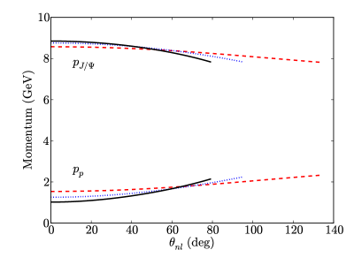
Figure 2: (Color online) Dependence of the momenta of struck nucleon and $J/\Psi$ meson on the momentum and direction of the recoil nucleon, given $q_{0}=10~{}\mathrm{GeV}$ and $t=-2.23~{}\mathrm{GeV}^{2}$, for the reaction (1). The curves have the same meaning as in Fig. 1.

For light vector mesons, such a regime can be established if one considers kinematics where the momentum transfer at the $\gamma N\rightarrow VN$ vertex is sufficiently large, namely $-t\geq 1~{}\mathrm{GeV}^{2}$. As Fig. 1 demonstrates, for $t=-1.2~{}\mathrm{GeV}^{2}$ both the $\phi$ meson and the proton are sufficiently energetic for different values of the neutron momentum. The photon energy in this figure is $5~{}\mathrm{GeV}$ and the value of $t$ is chosen on the proven feasibility of probing $\phi$ photoproduction at this $t$ value in coherent processes at Jefferson LabMibe et al. (2007). Hereafter, we represent the neutron direction using the angle it makes with respect to the direction of the momentum transfer.

For heavier mesons such as $J/\Psi$, the eikonal regime is established naturally near threshold kinematics due to the large value of $-t_{\mathrm{thr.}}$ (as calculated for a stationary proton target). This can be seen in Fig. 2, where the momenta of the proton and $J/\Psi$ meson are presented for different values of the neutron momentum, given a near-threshold photon energy of $10~{}\mathrm{GeV}$ (the threshold being $8.2~{}\mathrm{GeV}$), and $t=t_{\mathrm{thr.}}$.

Provided the eikonal regime is established, we can use a diagrammatic approach to calculate the reaction amplitude, which is expanded in the number of rescatterings (see e.g. Sargsian (2001)). In such an expansion, we will have only three categories of scattering amplitudes: a 0th order term corresponding to the plane wave impulse approximation, and 1st and 2nd order terms corresponding to terms with one or two hadronic rescatterings.

III Calculation of the scattering amplitude and cross section

We denote the four-momenta of the deuteron, photon, vector meson, proton, and neutron as $p_{d}=(E_{d},\mathbf{p}_{d})$, $q=(q_{0},\mathbf{q})$, $p_{V}=(E_{V},\mathbf{p}_{V})$ $p_{p}=(E_{p},\mathbf{p}_{p})$ and $p_{n}=(E_{n},\mathbf{p}_{n})$, respectively. We also denote the “initial” momenta of the proton and neutron within the deuteron (prior to vector meson photoproduction) as $p^{\prime}_{p}$ and $p^{\prime}_{n}$, respectively. The four-momentum transfer to the deuteron is defined as

$$l^{\mu}=(l_{0},\mathbf{l})\equiv(q_{0}-E_{V},\mathbf{q}-\mathbf{p}_{V})$$ (2)

with $t=l^{2}$. As was mentioned above, the direction of the outgoing neutron is defined by the angle it makes with the momentum transfer $\mathbf{l}$, and is denoted $\theta_{nl}$.

The general expression for the differential cross-section of the reaction (1) is:

$$d\sigma=\frac{1}{4(q\cdot p_{d})}\overline{\mid\mathcal{M}\mid^{2}}(2\pi)^{4}\delta^{4}(q+p_{d}-p_{V}-p_{p}-p_{n})\frac{d^{3}\mathbf{p}_{V}}{(2\pi)^{3}2E_{V}}\frac{d^{3}\mathbf{p}_{p}}{(2\pi)^{3}2E_{p}}\frac{d^{3}\mathbf{p}_{n}}{(2\pi)^{3}2E_{n}},$$ (3)

where we sum over the final and average over the initial particle polarizations. In our approach, the Feynman amplitude $\mathcal{M}$ is expanded in terms of the number of hadronic rescatterings (see e.g. Sargsian (2001))

$$\mathcal{M}=\mathcal{M}_{0}+\mathcal{M}_{1}+\mathcal{M}_{2},$$ (4)

where, $\mathcal{M}_{0}$, $\mathcal{M}_{1}$ and $\mathcal{M}_{2}$ correspond respectively to PWIA and the single and double rescattering amplitudes. These amplitudes will be calculated within the virtual nucleon approximation (VNA), in which only the $pn$ component of the deuteron wave-function and only the positive-energy pole of each nucleon’s propagator is considered. This allows us to relate the covariant $d\rightarrow pn$ transition amplitude to the deuteron wave-function with a virtual struck and an on-shell spectator nucleon (see e.g. Buck and Gross (1979)). Because the non-nucleonic components of the deuteron and the negative-energy poles of the nucleon propagators are neglected, the deuteron wave-fuction does not saturate the momentum sum rule. However, the relativistic normalization of the wave-function is fixed by baryon number conservation (see e.g. Frankfurt and Strikman (1976)). Previous estimatesSargsian (2010) demonstrate that this approximation works reasonably well for deuteron internal momenta $\lesssim 700~{}\mathrm{MeV/c}$, which will be considered as a kinematical limit for the present calculations.

III.1 Plane Wave Impulse Approximation

In plane wave impulse approximation (PWIA), we neglect the final state interactions between outgoing hadrons, treating them as plane waves (Fig. 3). The covariant scattering amplitude $\mathcal{M}_{0}$ within PWIA can be calculated based on effective Feynman diagram rules (see e.g. Sargsian (2001)) which give:

$$\mathcal{M}^{(\lambda_{V}\lambda_{p}\lambda_{n};\lambda_{\gamma}\lambda_{d})}_{0} =-\bar{u}^{(\lambda_{p})}(\mathbf{p}_{p})\bar{u}^{(\lambda_{n})}(\mathbf{p}_{n}){\phi^{\dagger}}^{(\lambda_{V})}_{\nu}(\mathbf{p}_{V})\Gamma^{\mu\nu}_{\gamma N\rightarrow VN}\epsilon_{\mu}^{(\lambda_{\gamma})}(q)$$

$$\times\frac{\not{p}^{\prime}_{p}+m_{N}}{p^{\prime 2}_{p}-m_{N}^{2}+i\epsilon}\Gamma_{dpn}\chi_{d}^{(\lambda_{d})}(\mathbf{p}_{d}).$$ (5)

Here, $\Gamma_{dpn}$ and $\Gamma^{\mu\nu}_{\gamma N\rightarrow VN}$ are the covariant vertices for the transitions $d\rightarrow pn$ and $\gamma N\rightarrow VN$. The spin wave-functions of the deuteron, nucleons, photon and vector meson are denoted $\chi_{d}$, $u$, $\epsilon_{\mu}$, and $\phi_{\nu}$, respectively. The spin degree of freedom of each particle is identified by a superscript in parentheses.

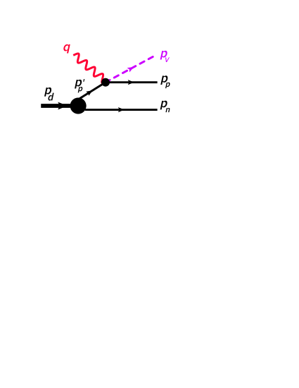
Figure 3: (Color online) Feynman diagram for PWIA scattering.

As was discussed above, we evaluate Eq. (5) by considering only the positive-energy pole in the bound nucleon propagator. Then, in accordance with VNA we use the approximate completeness relation $\not{p}^{\prime}_{p}+m_{N}\approx\sum_{\lambda^{\prime}_{p}}u^{(\lambda^{\prime}_{p})}(\mathbf{p}^{\prime}_{p})\bar{u}^{(\lambda^{\prime}_{p})}(\mathbf{p}^{\prime}_{p})$ in which the four-momentum of the struck nucleon is defined through the off-shell kinematic condition $p^{\prime}_{p}=p_{d}-p_{n}$, meaning that $p^{\prime 2}_{p}\neq m_{N}^{2}$ (see e.g. Sargsian (2010)). This allows us to introduce the deuteron-wave-function within VNASargsian (2010) as

$$\Psi_{d}^{(\lambda_{d};\lambda_{1}\lambda_{2})}(\mathbf{p})=-\frac{\bar{u}^{(\lambda_{1})}(\mathbf{p}_{1})\bar{u}^{(\lambda_{2})}(\mathbf{p}_{2})}{p_{1}^{2}-m_{N}^{2}}\frac{\Gamma_{dpn}\chi_{d}^{(\lambda_{d})}(\mathbf{p}_{d})}{\sqrt{2(2\pi)^{3}2E_{2}}}$$ (6)

where $\mathbf{p}=\frac{1}{2}(\mathbf{p}_{1}-\mathbf{p}_{2})$ and $\mathbf{p}_{d}=\mathbf{p}_{1}+\mathbf{p}_{2}$. Further calculations we perform in the lab frame (i.e. the deuteron rest frame), for which $\mathbf{p}=\mathbf{p}_{1}=-\mathbf{p}_{2}$.

Using Eq. (6) and introducing the invariant Feynman amplitude for vector meson photoproduction from the struck nucleon, i.e.

$$\mathcal{M}^{(\lambda_{V}\lambda_{p};\lambda_{\gamma}\lambda^{\prime}_{p})}_{\gamma N\rightarrow VN}(s_{\gamma N^{*}},t_{\gamma N^{*}})=\bar{u}^{(\lambda_{p})}(\mathbf{p}_{p}){\phi^{\dagger}}^{(\lambda_{V})}_{\nu}(\mathbf{p}_{V})\Gamma^{\mu\nu}_{\gamma N\rightarrow VN}\epsilon_{\mu}(q)u^{(\lambda^{\prime}_{p})}(\mathbf{p}^{\prime}_{p})$$ (7)

into Eq. (5), we find the PWIA amplitude to be

$$\mathcal{M}^{(\lambda_{V}\lambda_{p}\lambda_{n};\lambda_{\gamma}\lambda_{d})}_{0}=\sqrt{2(2\pi)^{3}2E_{p}}\sum_{\lambda^{\prime}_{p}}\mathcal{M}^{(\lambda_{V}\lambda_{p};\lambda_{\gamma}\lambda^{\prime}_{p})}_{\gamma N\rightarrow VN}(s_{\gamma N^{*}},t_{\gamma N^{*}})\Psi_{d}^{(\lambda_{d};\lambda^{\prime}_{p}\lambda_{n})}(\mathbf{p}_{n})$$ (8)

where $s_{\gamma N^{*}}$ and $t_{\gamma N^{*}}$ are the Mandelstam variables at the $\gamma N\rightarrow VN$ vertex. Note that the vector meson photoproduction amplitude that enters above is half-off-shell since the struck nucleon is initially in a virtual state. In these calculations, however, we use on-shell spinors for the bound nucleon and account for off-shell effects only kinematically by identifying the four-momentum of the bound nucleon as $p^{\prime}_{p}=p_{d}-p_{n}$. Earlier estimatesSargsian (2010) demonstrated this approximation to be reasonable when $\frac{|\mathbf{p}^{\prime}_{p}|}{\sqrt{-t}},\frac{|\mathbf{p}^{\prime}_{p}|}{\sqrt{s}}\ll 1$, both of which are satisfied here.

III.2 Single Rescattering Contribution

Within GEA, there are four single rescattering processes to consider (Fig. 4). The processes can be separated into two groups. In the first group (Fig. 4(a,b)), the proton receives its large momentum due to a hard photoproduction vertex, while in the second (Fig. 4(c,d)) its large momentum comes from a hard rescattering vertex.

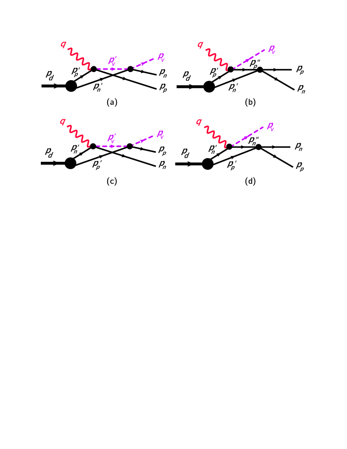
Figure 4: (Color online) Feynman diagrams for single rescattering contribution.

While the first three diagrams in Fig. 4 can be identified as having one hard and one soft rescattering vertex, the fourth one requires two hard vertices in order to provide a large momentum to both the vector meson and proton. In principle, a possible “one-hard”and “one-soft” scenario can be realized for the fourth diagram if the high momentum of the intermediate neutron is transferred to the final proton by means of a small angle charge interchange reaction. However, this contribution is negligible due to the pion exchange nature of charge interchange scattering at the considered energies, which results in an overall contribution that decreases with $s_{pn}$ and contributes at most a few percent in the forward direction.

It is worth noting that due to antisymmetry of the nuclear wave function, the amplitude of Fig. 4(c) enters with the opposite sign relative to the amplitude of Fig. 4(a). However its contribution will be suppressed for near-threshold production of heavy vector mesons (such as $J/\Psi$), since the high $-t_{\mathrm{thr.}}$ of the photoproduction reaction will make the first vertex hard. Thus we expect appreciable contribution from Fig. 4(c) only for higher photon energies, or when the produced vector meson is light.

We will calculate only the contributions of diagrams Fig. 4(a,b,c), for which we use effective Feynman rules (see Ref. Sargsian (2001)). Denoting the invariant amplitudes of the processes as $\mathcal{M}_{1a}$, $\mathcal{M}_{1b}$ and $\mathcal{M}_{1c}$, we obtain

$$\mathcal{M}_{1a}^{(\lambda_{V},\lambda_{p},\lambda_{n};\lambda_{\gamma},\lambda_{d})} =-\bar{u}^{(\lambda_{p})}(\mathbf{p}_{p})\bar{u}^{(\lambda_{n})}(\mathbf{p}_{n})\phi_{\pi}^{(\lambda_{V})}(\mathbf{p}_{V})\int\frac{d^{4}p_{n}^{\prime}}{(2\pi)^{4}i}\bigg{[}\Gamma^{\rho\pi}_{VN\rightarrow VN}\frac{G_{\nu\rho}(p_{V}^{\prime})}{(p_{V}^{\prime})^{2}-m_{V}^{2}+i\epsilon}\Gamma^{\mu\nu}_{\gamma N\rightarrow VN}\epsilon_{\mu}^{(\lambda_{\gamma})}$$

$$\times\frac{\not{p}_{p}^{\prime}+m_{N}}{(p_{p}^{\prime})^{2}-m_{N}^{2}+i\epsilon}\frac{\not{p}_{n}^{\prime}+m_{N}}{(p_{n}^{\prime})^{2}-m_{N}^{2}+i\epsilon}\Gamma_{dpn}\chi_{d}^{(\lambda_{d})}\bigg{]}$$ (9)

$$\mathcal{M}_{1b}^{(\lambda_{V},\lambda_{p},\lambda_{n};\lambda_{\gamma},\lambda_{d})} =-\bar{u}^{(\lambda_{p})}(\mathbf{p}_{p})\bar{u}^{(\lambda_{n})}(\mathbf{p}_{n})\phi_{\nu}^{(\lambda_{V})}(\mathbf{p}_{V})\int\frac{d^{4}p_{p}^{\prime}}{(2\pi)^{4}i}\bigg{[}\Gamma_{pn\rightarrow pn}\frac{\not{p}_{p}^{\prime\prime}+m_{N}}{(p_{p}^{\prime\prime})^{2}-m_{N}^{2}+i\epsilon}\frac{\not{p}_{n}^{\prime}+m_{N}}{(p_{n}^{\prime})^{2}-m_{N}^{2}+i\epsilon}$$

$$\times\Gamma^{\mu\nu}_{\gamma N\rightarrow VN}\epsilon_{\mu}^{(\lambda_{\gamma})}\frac{\not{p}_{p}^{\prime}+m_{N}}{(p_{p}^{\prime})^{2}-m_{N}^{2}+i\epsilon}\Gamma_{dpn}\chi_{d}^{(\lambda_{d})}\bigg{]}$$ (10)

$$\mathcal{M}_{1c}^{(\lambda_{V},\lambda_{p},\lambda_{n};\lambda_{\gamma},\lambda_{d})} =-\bar{u}^{(\lambda_{p})}(\mathbf{p}_{p})\bar{u}^{(\lambda_{n})}(\mathbf{p}_{n})\phi_{\pi}^{(\lambda_{V})}(\mathbf{p}_{V})\int\frac{d^{4}p_{p}^{\prime}}{(2\pi)^{4}i}\bigg{[}\Gamma^{\rho\pi}_{VN\rightarrow VN}\frac{G_{\nu\rho}(p_{V}^{\prime})}{(p_{V}^{\prime})^{2}-m_{V}^{2}+i\epsilon}\Gamma^{\mu\nu}_{\gamma N\rightarrow VN}\epsilon_{\mu}^{(\lambda_{\gamma})}$$

$$\times\frac{\not{p}_{p}^{\prime}+m_{N}}{(p_{p}^{\prime})^{2}-m_{N}^{2}+i\epsilon}\frac{\not{p}_{n}^{\prime}+m_{N}}{(p_{n}^{\prime})^{2}-m_{N}^{2}+i\epsilon}\Gamma_{dpn}\chi_{d}^{(\lambda_{d})}\bigg{]}$$ (11)

where $G_{\mu\nu}(p_{V})=g_{\mu\nu}-(p_{V})_{\mu}(p_{V})_{\nu}/m_{V}^{2}$ is the propagator of the intermediate vector meson. The momentum notations of intermediate particles are given in Fig. 4.

Our derivations follow the prescription of virtual nucleon approximation (cf. Sec. III.1 and Ref. Sargsian (2010)), in which the spectator to the photoproduction sub-reaction is placed on its mass shell by considering only the positive-energy pole in the spectator energy integration, i.e. we take

$$\int\frac{dp^{\prime 0}_{p/n}}{p^{\prime 2}_{p/n}-m_{N}^{2}+i\epsilon}=-i\frac{2\pi}{2E^{\prime}_{p/n}}$$ (12)

where $E^{\prime}_{p/n}=+\sqrt{m_{N}^{2}+\mathbf{p}^{\prime 2}_{p/n}}$. Since this integration places the spectator on its mass shell, the completeness relation $\not{p}^{\prime}_{p/n}+m_{N}=\sum_{\lambda^{\prime}_{p/n}}u^{(\lambda^{\prime}_{p/n})}(\mathbf{p}^{\prime}_{p/n})\bar{u}^{(\lambda^{\prime}_{p/n})}(\mathbf{p}^{\prime}_{p/n})$ is exact. This, together with the approximate completeness relation used for the off-shell nucleon propagator allows us to introduce the deuteron wave-function of Eq. (6) into the rescattering amplitudes as follows:

$$\mathcal{M}_{1a}^{(\lambda_{V},\lambda_{p},\lambda_{n};\lambda_{\gamma},\lambda_{d})} =-\bar{u}^{(\lambda_{p})}(\mathbf{p}_{p})\bar{u}^{(\lambda_{n})}(\mathbf{p}_{n})\phi_{\pi}^{(\lambda_{V})}(\mathbf{p}_{V})\sum_{\lambda_{p}^{\prime},\lambda_{n}^{\prime}}\int\frac{d^{3}\mathbf{p}_{n}^{\prime}}{(2\pi)^{3}}\bigg{[}\sqrt{\frac{2(2\pi)^{3}}{2E_{n}^{\prime}}}\Gamma^{\rho\pi}_{VN\rightarrow VN}u^{(\lambda_{n}^{\prime})}(\mathbf{p}_{n}^{\prime})$$

$$\times\frac{G_{\nu\rho}(p_{V}^{\prime})}{(p_{V}^{\prime})^{2}-m_{V}^{2}+i\epsilon}\Gamma^{\mu\nu}_{\gamma N\rightarrow VN}\epsilon_{\mu}^{(\lambda_{\gamma})}u^{(\lambda_{p}^{\prime})}(\mathbf{p}_{p}^{\prime})\Psi_{d}^{(\lambda_{p}^{\prime},\lambda_{n}^{\prime};\lambda_{d})}(\mathbf{p}_{n}^{\prime})\bigg{]}$$ (13)

$$\mathcal{M}_{1b}^{(\lambda_{V},\lambda_{p},\lambda_{n};\lambda_{\gamma},\lambda_{d})} =-\bar{u}^{(\lambda_{p})}(\mathbf{p}_{p})\bar{u}^{(\lambda_{n})}(\mathbf{p}_{n})\phi_{\nu}^{(\lambda_{V})}(\mathbf{p}_{V})\int\frac{d^{3}\mathbf{p}_{n}^{\prime}}{(2\pi)^{3}}\bigg{[}\sqrt{\frac{2(2\pi)^{3}}{2E_{n}^{\prime}}}\Gamma_{pn\rightarrow pn}u^{(\lambda_{n}^{\prime})}(\mathbf{p}_{n}^{\prime})$$

$$\times\frac{\not{p}_{p}^{\prime\prime}+m_{N}}{(p_{p}^{\prime\prime})^{2}-m_{N}^{2}+i\epsilon}\Gamma^{\mu\nu}_{\gamma N\rightarrow VN}\epsilon_{\mu}^{(\lambda_{\gamma})}u^{(\lambda_{p}^{\prime})}(\mathbf{p}_{p}^{\prime})\Psi_{d}^{(\lambda_{p}^{\prime},\lambda_{n}^{\prime};\lambda_{d})}(\mathbf{p}_{n}^{\prime})\bigg{]}$$ (14)

$$\mathcal{M}_{1c}^{(\lambda_{V},\lambda_{p},\lambda_{n};\lambda_{\gamma},\lambda_{d})} =-\bar{u}^{(\lambda_{p})}(\mathbf{p}_{p})\bar{u}^{(\lambda_{n})}(\mathbf{p}_{n})\phi_{\pi}^{(\lambda_{V})}(\mathbf{p}_{V})\int\frac{d^{3}\mathbf{p}_{p}^{\prime}}{(2\pi)^{3}}\bigg{[}\sqrt{\frac{2(2\pi)^{3}}{2E_{p}^{\prime}}}\Gamma^{\rho\pi}_{VN\rightarrow VN}u^{(\lambda_{p}^{\prime})}(\mathbf{p}_{p}^{\prime})$$

$$\times\frac{G_{\nu\rho}(p_{V}^{\prime})}{(p_{V}^{\prime})^{2}-m_{V}^{2}+i\epsilon}\Gamma^{\mu\nu}_{\gamma N\rightarrow VN}\epsilon_{\mu}^{(\lambda_{\gamma})}u^{(\lambda_{n}^{\prime})}(\mathbf{p}_{n}^{\prime})\Psi_{d}^{(\lambda_{n}^{\prime},\lambda_{p}^{\prime};\lambda_{d})}(\mathbf{p}_{p}^{\prime})\bigg{]}.$$ (15)

Note that, due to the fact the deuteron wave-function is antisymmetric with respect to a $p$-$n$ permutation, the amplitude $\mathcal{M}_{1c}$ has a negative sign relative to $\mathcal{M}_{1a}$ and $\mathcal{M}_{1b}$.

We consider next the remaining “fast” propagator in each amplitude: the vector meson propagators for $\mathcal{M}_{1a}$ and $\mathcal{M}_{1c}$ and the proton propagator for $\mathcal{M}_{1b}$. In each case we introduce the momentum transfer at the rescattering vertex as $K=p_{n}-p_{n}^{\prime}$ and rewrite the propagators in terms of it.

For the propagator in $\mathcal{M}_{1a}$, we obtain

$$(p_{V}^{\prime})^{2}-m_{V}^{2}+i\epsilon =(p_{V}+p_{n}-p_{n}^{\prime})^{2}-m_{V}^{2}+i\epsilon=(p_{V}+K)^{2}-m_{V}^{2}+i\epsilon$$

$$=2p_{V,z}\left(\Delta_{1a}-K_{z}+i\epsilon\right),$$ (16)

where

$$\Delta_{1a}=\frac{K^{2}+2K_{0}E_{V}-2\mathbf{K}_{\perp}\cdot\mathbf{p}_{V}}{2p_{V,z}}.$$ (17)

To proceed with the integration, we use the fact that the rescattering amplitude is dominated by small angle scattering. This means that $K_{z}^{2}\ll\mathbf{K}_{\perp}^{2}$, so $K_{0}$ and $K^{2}$ are approximately equal to their $K_{z}=0$ values. Moreover, $\frac{\partial\Delta_{1a}}{\partial K_{z}}\sim\frac{K_{z}}{p_{V,z}}\ll 1$ so we may treat $\Delta_{1a}$ as independent of $K_{z}$, effectively linearizing the denominator of Eq. (16). With this in mind, and the fact that the integration over $\mathbf{p}_{n}^{\prime}$ in Eq. (13) can be rewritten as an integration over $\mathbf{K}$, the $dK_{z}$ integration can be performed using

$$\int\frac{f(z)dz}{\Delta-z+i\epsilon}=-i\pi f(\Delta)+\mathcal{P}\int\frac{f(z)dz}{\Delta-z},$$ (18)

where the symbol $\mathcal{P}$ indicates that the Cauchy principal value of the integral is to be taken.

In applying the decomposition (18) to $\mathcal{M}_{1a}$, we can separate $\mathcal{M}_{1a}$ into on-shell and off-shell parts, since the condition $\Delta_{1a}=K_{z}$ imposed by the delta function corresponds to the on-shell condition for the intermediate vector meson—i.e. it happens when $(p_{V}^{\prime})^{2}=m_{V}^{2}$. We shall henceforth refer to this part of $\mathcal{M}_{1a}$ as the pole term. Because, in this term, the internal vector meson line is on its mass shell, we can now use the completeness relation $G_{\nu\rho}(p_{V}^{\prime})=\sum_{\lambda_{V}^{\prime}}{\phi_{\nu}}^{(\lambda_{V}^{\prime})}(\mathbf{p}_{V}^{\prime}){\phi_{\rho}^{*}}^{(\lambda_{V}^{\prime})}(\mathbf{p}_{V}^{\prime})$ and gather terms together into the invariant amplitudes for the $\gamma N\rightarrow VN$ and $VN\rightarrow VN$ transitions:

$$\mathcal{M}_{1a,\mathrm{pole}}^{(\lambda_{V},\lambda_{p},\lambda_{n};\lambda_{\gamma},\lambda_{d})} =\frac{i}{4p_{V,z}}\sum_{\lambda_{V}^{\prime},\lambda_{p}^{\prime},\lambda_{n}^{\prime}}\int\frac{d^{2}\mathbf{K}_{\perp}}{(2\pi)^{2}}\bigg{[}\sqrt{\frac{2(2\pi)^{3}}{2E_{n}^{\prime}}}\mathcal{M}_{VN\rightarrow VN}^{(\lambda_{V},\lambda_{n};\lambda_{V}^{\prime},\lambda_{n}^{\prime})}(s_{VN},t_{VN})$$

$$\times\mathcal{M}_{\gamma N\rightarrow VN}^{(\lambda_{V}^{\prime},\lambda_{p};\lambda_{\gamma},\lambda_{p}^{\prime})}(s_{\gamma N^{*}},t_{\gamma N^{*}})\Psi_{d}^{(\lambda_{p}^{\prime},\lambda_{n}^{\prime};\lambda_{d})}(p_{n,z}-\Delta_{1a},\mathbf{p}_{n,\perp}-\mathbf{K}_{\perp})\bigg{]}.$$ (19)

Here, as in PWIA the invariant amplitudes appearing on the RHS are functions of the Mandelstam variables for their respective transitions.

For the other two rescattering amplitudes, similar decompositions of the fast propagators are possible. For $\mathcal{M}_{1b}$, we have

$$(p_{p}^{\prime})^{2}-m_{N}^{2}+i\epsilon =(p_{p}+p_{n}-p_{n}^{\prime})^{2}-m_{N}^{2}+i\epsilon=(p_{p}+K)^{2}-m_{N}^{2}+i\epsilon$$

$$=2p_{p,z}\left(\Delta_{1b}-K_{z}+i\epsilon\right),$$ (20)

where

$$\Delta_{1b}=\frac{K^{2}+2K_{0}E_{p}-2\mathbf{K}_{\perp}\cdot\mathbf{p}_{p}}{2p_{p,z}}.$$ (21)

This gives us a pole part of the amplitude equal to

$$\mathcal{M}_{1b,\mathrm{pole}}^{(\lambda_{V},\lambda_{p},\lambda_{n};\lambda_{\gamma},\lambda_{d})} =\frac{i}{4p_{p,z}}\sum_{\lambda_{p}^{\prime},\lambda_{p}^{\prime\prime},\lambda_{n}^{\prime}}\int\frac{d^{2}\mathbf{K}_{\perp}}{(2\pi)^{2}}\bigg{[}\sqrt{\frac{2(2\pi)^{3}}{2E_{n}^{\prime}}}\mathcal{M}_{pn\rightarrow pn}^{(\lambda_{p},\lambda_{n};\lambda_{p}^{\prime\prime},\lambda_{n}^{\prime})}(s_{pn},t_{pn})$$

$$\times\mathcal{M}_{\gamma N\rightarrow VN}^{(\lambda_{V},\lambda_{p}^{\prime\prime};\lambda_{\gamma},\lambda_{p}^{\prime})}(s_{\gamma N^{*}},t_{\gamma N^{*}})\Psi_{d}^{(\lambda_{p}^{\prime},\lambda_{n}^{\prime};\lambda_{d})}(p_{n,z}-\Delta_{1b},\mathbf{p}_{n,\perp}-\mathbf{K}_{\perp})\bigg{]}.$$ (22)

As for $\mathcal{M}_{1c}$, we have

$$(p_{V}^{\prime})^{2}-m_{V}^{2}+i\epsilon =(q+p_{n}^{\prime}-p_{n})^{2}-m_{V}^{2}+i\epsilon=(q-K)^{2}-m_{V}^{2}+i\epsilon$$

$$=2q_{0}\left(K_{z}-\Delta_{1c}+i\epsilon\right)$$ (23)

, where

$$\Delta_{1c}=\frac{m_{V}^{2}-K^{2}}{2q_{0}}+K_{0},$$ (24)

which gives us a pole part of the amplitude equal to

$$\mathcal{M}_{1c,\mathrm{pole}}^{(\lambda_{V},\lambda_{p},\lambda_{n};\lambda_{\gamma},\lambda_{d})} =\frac{i}{4q_{0}}\sum_{\lambda_{V}^{\prime},\lambda_{p}^{\prime},\lambda_{n}^{\prime}}\int\frac{d^{2}\mathbf{K}_{\perp}}{(2\pi)^{2}}\bigg{[}\sqrt{\frac{2(2\pi)^{3}}{2E_{p}^{\prime}}}\mathcal{M}_{VN\rightarrow VN}^{(\lambda_{V},\lambda_{p};\lambda_{V}^{\prime},\lambda_{p}^{\prime})}(s_{VN},t_{VN})$$

$$\times\mathcal{M}_{\gamma N\rightarrow VN}^{(\lambda_{V}^{\prime},\lambda_{n};\lambda_{\gamma},\lambda_{n}^{\prime})}(s_{\gamma N^{*}},t_{\gamma N^{*}})\Psi_{d}^{(\lambda_{n}^{\prime},\lambda_{p}^{\prime};\lambda_{d})}(-p_{n,z}+\Delta_{1c},-\mathbf{p}_{n,\perp}+\mathbf{K}_{\perp})\bigg{]}.$$ (25)

For the principal value (PV) parts of each amplitude, we simplify the notation by introducing half-off-shell $VN\rightarrow VN$ and $pn\rightarrow pn$ amplitudes that allow us to write the following:

$$\mathcal{M}_{1a,\mathrm{pv}}^{(\lambda_{V},\lambda_{p},\lambda_{n};\lambda_{\gamma},\lambda_{d})} =\frac{1}{2p_{V,z}}\sum_{\lambda_{V}^{\prime},\lambda_{p}^{\prime},\lambda_{n}^{\prime}}\int\frac{d^{2}\mathbf{K}_{\perp}}{(2\pi)^{2}}\mathcal{P}\int\frac{dK_{z}}{2\pi}\bigg{[}\sqrt{\frac{2(2\pi)^{3}}{2E_{n}^{\prime}}}\mathcal{M}_{V^{*}N\rightarrow VN}^{(\lambda_{V}\lambda_{n};\lambda_{V}^{\prime}\lambda_{n}^{\prime})}(s_{V^{*}N},t_{V^{*}N})$$

$$\times\mathcal{M}_{\gamma N^{*}\rightarrow VN}^{(\lambda_{V}^{\prime}\lambda_{p};\lambda_{\gamma}\lambda_{p}^{\prime})}(s_{\gamma N^{*}},t_{\gamma N^{*}})\frac{\Psi_{d}^{(\lambda_{p}^{\prime},\lambda_{n}^{\prime};\lambda_{d})}(p_{n,z}-\Delta_{1a},\mathbf{p}_{n,\perp}-\mathbf{K}_{\perp})}{K_{z}-\Delta_{1a}}\bigg{]}$$ (26)

$$\mathcal{M}_{1b,\mathrm{pv}}^{(\lambda_{V},\lambda_{p},\lambda_{n};\lambda_{\gamma},\lambda_{d})} =\frac{1}{2p_{p,z}}\sum_{\lambda_{V}^{\prime},\lambda_{p}^{\prime},\lambda_{n}^{\prime}}\int\frac{d^{2}\mathbf{K}_{\perp}}{(2\pi)^{2}}\mathcal{P}\int\frac{dK_{z}}{2\pi}\bigg{[}\sqrt{\frac{2(2\pi)^{3}}{2E_{n}^{\prime}}}\mathcal{M}_{p^{*}n\rightarrow pn}^{(\lambda_{p}\lambda_{n};\lambda_{p}^{\prime\prime}\lambda_{n}^{\prime})}(s_{p^{*}n},t_{p^{*}n})$$

$$\times\mathcal{M}_{\gamma N^{*}\rightarrow VN}^{(\lambda_{V}\lambda_{p^{\prime}\prime};\lambda_{\gamma}\lambda_{p}^{\prime})}(s_{\gamma N^{*}},t_{\gamma N^{*}})\frac{\Psi_{d}^{(\lambda_{p}^{\prime},\lambda_{n}^{\prime};\lambda_{d})}(p_{n,z}-\Delta_{1b},-\mathbf{p}_{n,\perp}+\mathbf{K}_{\perp})}{K_{z}-\Delta_{1b}}\bigg{]}$$ (27)

$$\mathcal{M}_{1c,\mathrm{pv}}^{(\lambda_{V},\lambda_{p},\lambda_{n};\lambda_{\gamma},\lambda_{d})} =-\frac{1}{2q_{0}}\sum_{\lambda_{V}^{\prime},\lambda_{p}^{\prime},\lambda_{n}^{\prime}}\int\frac{d^{2}\mathbf{K}_{\perp}}{(2\pi)^{2}}\mathcal{P}\int\frac{dK_{z}}{2\pi}\bigg{[}\sqrt{\frac{2(2\pi)^{3}}{2E_{p}^{\prime}}}\mathcal{M}_{V^{*}N\rightarrow VN}^{(\lambda_{V}\lambda_{p};\lambda_{V}^{\prime}\lambda_{p}^{\prime})}(s_{V^{*}N},t_{V^{*}N})$$

$$\times\mathcal{M}_{\gamma N^{*}\rightarrow VN}^{(\lambda_{V}^{\prime}\lambda_{n};\lambda_{\gamma}\lambda_{n}^{\prime})}(s_{\gamma N^{*}},t_{\gamma N^{*}})\frac{\Psi_{d}^{(\lambda_{n}^{\prime},\lambda_{p}^{\prime};\lambda_{d})}(-p_{n,z}+\Delta_{1c},\mathbf{p}_{n,\perp}-\mathbf{K}_{\perp})}{K_{z}-\Delta_{1c}}\bigg{]},$$ (28)

where we have written $V^{*}$ and $p^{*}$ to indicate that these particles are off-shell in their intermediate states. We will estimate these amplitudes numerically by substituting off-shell rescattering amplitudes with on-shell counterparts evaluated at off-shell kinematics. However, it is important to note that our approach can only be used to probe the $VN\rightarrow VN$ amplitude when the principal value parts are negligible.

III.3 Double Rescattering Contribution

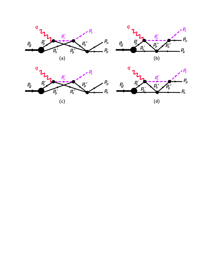
Figure 5: (Color online) Feynman diagrams for double rescattering contribution.

The last term in Eq. (4) corresponds to double rescattering contributions (Fig. 5). They, like the single rescattering processes, can be split into two groups. The first group (Fig. 5(a,b)) correspond to hard vector meson production from the proton, followed by two consecutive soft rescatterings from the slow neutron. The two remaining diagrams (Fig. 5(c,d)) correspond to vector meson production from the neutron, and provide the proton with a large final momentum by means of a hard rescattering vertex.

It is worth noting that, for heavy vector meson production near threshold, the last two diagrams are negligible due to the large $-t$ involved in both the photoproduction vertex and one of the proton rescatterings. However, the contribution of Fig. 5(c) becomes relevant for high energies. The contribution of Fig. 5(d) remains negligible at high energies due to the fact that it contains an intermediate state with a slow proton-neutron pair, the momentum of which is integrated over. This warrants the application of a closure condition as an approximation, which results in a cancelation of any correction this diagram would make to the contribution of Fig. 4(b).

In calculating the diagrams Fig. 5(a,b,c), we will concentrate only on the contributions from the pole terms of the fast hadron propagators that contain on-shell $p$-$n$ and $V$-$N$ scattering amplitudes. As discussed in the previous section, this is justified by focusing only on kinematics where the principal value contributions are a small correction. Since one would expect that $\mathcal{M}_{2}\ll\mathcal{M}_{1}$, the PV parts of $\mathcal{M}_{2}$ should be significantly smaller than the overall amplitude.

Applying the effective Feynman rules and performing the loop integrations in accordance with the same prescription used for the single rescattering amplitudes, we find the pole terms of the diagrams in Fig. 5(a,b,c) to be

$$\mathcal{M}_{2a}^{(\lambda_{V},\lambda_{p},\lambda_{n};\lambda_{\gamma},\lambda_{d})} =-\frac{1}{4p_{p,z}p_{V,z}}\sum_{\mathrm{spins}}\int\frac{d^{2}\mathbf{K}}{(2\pi)^{2}}\int\frac{d^{2}\mathbf{K}^{\prime}}{(2\pi)^{2}}\bigg{[}\sqrt{\frac{2(2\pi)^{3}}{2E_{n}^{\prime}}}\frac{1}{2E_{n}^{\prime\prime}}\mathcal{M}_{pn\rightarrow pn}^{(\lambda_{p},\lambda_{n};\lambda_{p}^{\prime\prime},\lambda_{n}^{\prime\prime})}(p_{p},p_{n};p_{p}^{\prime\prime},p_{n}^{\prime\prime})$$

$$\times\mathcal{M}_{VN\rightarrow VN}^{(\lambda_{V},\lambda_{n}^{\prime\prime};\lambda_{V}^{\prime},\lambda_{n}^{\prime})}(p_{V},p_{n}^{\prime\prime};p_{V}^{\prime},p_{n}^{\prime})\mathcal{M}_{\gamma N\rightarrow VN}^{(\lambda_{V}^{\prime},\lambda_{p}^{\prime\prime};\lambda_{\gamma},\lambda_{p}^{\prime})}(p_{V}^{\prime},p_{p}^{\prime\prime};p_{\gamma},p_{p}^{\prime})$$

$$\times\Psi_{d}^{(\lambda_{p}^{\prime},\lambda_{n}^{\prime};\lambda_{d})}(p_{n,z}-\Delta_{2a}-\Delta_{2a}^{\prime};\mathbf{p}_{n,\perp}-\mathbf{K}_{\perp}-\mathbf{K}^{\prime}_{\perp})\bigg{]}$$ (29)

$$\mathcal{M}_{2b}^{(\lambda_{V},\lambda_{p},\lambda_{n};\lambda_{\gamma},\lambda_{d})} =-\frac{1}{4p_{p,z}p_{V,z}}\sum_{\mathrm{spins}}\int\frac{d^{2}\mathbf{K}}{(2\pi)^{2}}\int\frac{d^{2}\mathbf{K}^{\prime}}{(2\pi)^{2}}\bigg{[}\sqrt{\frac{2(2\pi)^{3}}{2E_{n}^{\prime}}}\frac{1}{2E_{n}^{\prime\prime}}\mathcal{M}_{VN\rightarrow VN}^{(\lambda_{V},\lambda_{p};\lambda_{V}^{\prime},\lambda_{p}^{\prime\prime})}(p_{V},p_{p};p_{V}^{\prime},p_{p}^{\prime\prime})$$

$$\times\mathcal{M}_{pn\rightarrow pn}^{(\lambda_{p},\lambda_{n}^{\prime\prime};\lambda_{p}^{\prime\prime},\lambda_{n}^{\prime})}(p_{p},p_{n}^{\prime\prime};p_{p}^{\prime\prime},p_{n}^{\prime})\mathcal{M}_{\gamma N\rightarrow VN}^{(\lambda_{V}^{\prime},\lambda_{p}^{\prime\prime};\lambda_{\gamma},\lambda_{p}^{\prime})}(p_{V}^{\prime},p_{p}^{\prime\prime};p_{\gamma},p_{p}^{\prime})$$

$$\times\Psi_{d}^{(\lambda_{p}^{\prime},\lambda_{n}^{\prime};\lambda_{d})}(p_{n,z}-\Delta_{2b}-\Delta_{2b}^{\prime};\mathbf{p}_{n,\perp}-\mathbf{K}_{\perp}-\mathbf{K}^{\prime}_{\perp})\bigg{]}$$ (30)

$$\mathcal{M}_{2c}^{(\lambda_{V},\lambda_{p},\lambda_{n};\lambda_{\gamma},\lambda_{d})} =-\frac{1}{4q_{0}p_{p,z}}\sum_{\mathrm{spins}}\int\frac{d^{2}\mathbf{K}}{(2\pi)^{2}}\int\frac{d^{2}\mathbf{K}^{\prime}}{(2\pi)^{2}}\bigg{[}\sqrt{\frac{2(2\pi)^{3}}{2E_{p}^{\prime}}}\frac{1}{2E_{n}^{\prime\prime}}\mathcal{M}_{pn\rightarrow pn}^{(\lambda_{p},\lambda_{n};\lambda_{p}^{\prime\prime},\lambda_{n}^{\prime\prime})}(p_{p},p_{n};p_{p}^{\prime\prime},p_{n}^{\prime\prime})$$

$$\times\mathcal{M}_{VN\rightarrow VN}^{(\lambda_{V},\lambda_{p}^{\prime\prime};\lambda_{V}^{\prime},\lambda_{p}^{\prime})}(p_{V},p_{p}^{\prime\prime};p_{V}^{\prime},p_{p}^{\prime})\mathcal{M}_{\gamma N\rightarrow VN}^{(\lambda_{V}^{\prime},\lambda_{p}^{\prime\prime};\lambda_{\gamma},\lambda_{p}^{\prime})}(p_{V}^{\prime},p_{n}^{\prime\prime};p_{\gamma},p_{n}^{\prime})$$

$$\times\Psi_{d}^{(\lambda_{n}^{\prime},\lambda_{p}^{\prime};\lambda_{d})}(-p_{n,z}+\Delta_{2a}+\Delta_{2a}^{\prime};-\mathbf{p}_{n,\perp}+\mathbf{K}_{\perp}+\mathbf{K}^{\prime}_{\perp})\bigg{]}$$ (31)

where the delta factors are

$$\Delta_{2a} =\frac{K^{2}+2E_{p}K_{0}-2\mathbf{p}_{p}\cdot\mathbf{K}_{\perp}}{2p_{p,z}}$$ (32)

$$\Delta_{2a}^{\prime} =\frac{(K^{\prime})^{2}+2E_{V}K^{\prime}_{0}-2\mathbf{p}_{V}\cdot\mathbf{K}^{\prime}_{\perp}}{2p_{V,z}}$$ (33)

$$\Delta_{2b} =\frac{K^{2}+2E_{V}K_{0}-2\mathbf{p}_{V}\cdot\mathbf{K}_{\perp}}{2p_{V,z}}$$ (34)

$$\Delta_{2b}^{\prime} =\frac{(K^{\prime})^{2}+2E_{p}K^{\prime}_{0}-2\mathbf{p}_{p}\cdot\mathbf{K}^{\prime}_{\perp}}{2p_{p,z}}$$ (35)

$$\Delta_{2c} =\frac{K^{2}+2E_{p}K_{0}-2\mathbf{p}_{p}\cdot\mathbf{K}_{\perp}}{2p_{p,z}}$$ (36)

$$\Delta_{2c}^{\prime} =\frac{m_{V}^{2}-(K^{\prime})^{2}}{2q_{0}}+K^{\prime}_{0}$$ (37)

A derivation of these results can be found in the appendix.

III.4 Differential Cross Section

The differential cross section of reaction (1) is given by Eq. (3). We consider the particular case in which the vector meson and proton are detected, and the neutron is inferred from missing mass. In accordance with this, we integrate out the neutron momentum to obtain

$$d\sigma=\frac{\overline{|\mathcal{M}|^{2}}}{4\sqrt{s_{d}-M_{d}^{2}}}(2\pi)\delta((p_{d}+q-p_{V}-p_{p})^{2}-m_{N}^{2})\frac{d^{3}\mathbf{p}_{V}}{(2E_{V})(2\pi)^{3}}\frac{d^{3}\mathbf{p}_{p}}{(2E_{p})(2\pi)^{3}}.$$ (38)

We eliminate the remaining delta function by integrating over the magnitude of the proton momentum, which results in the following form of the differential cross-section:

$$\frac{d^{5}\sigma}{d^{3}\mathbf{p}_{V}d\Omega_{p}} = \frac{\overline{|\mathcal{M}|^{2}}}{4\sqrt{s_{d}-M_{d}^{2}}}\frac{1}{(2\pi)^{5}}\frac{1}{8E_{V}E_{1f}E_{n}}\frac{p_{p}^{3}}{|\mathbf{p}_{p}\cdot(\mathbf{v}_{p}-\mathbf{v}_{n})|}.$$ (39)

Here the outgoing nucleon velocities are $\mathbf{v}=\frac{\mathbf{p}}{E}$ and the total scattering amplitude is defined according to Eq. (4).

IV Numerical Estimates

For numerical estimates, it is convenient to express the invariant Feynman amplitude $\mathcal{M}_{AB\rightarrow CD}^{(\lambda_{C},\lambda_{D};\lambda_{A},\lambda_{B})}$ for the process $AB\rightarrow CD$ through the diffractive amplitude $f_{AB\rightarrow CD}^{(\lambda_{C},\lambda_{D};\lambda_{A},\lambda_{B})}$ in the following form:

$$\mathcal{M}_{AB\rightarrow X}^{(\lambda_{C},\lambda_{D};\lambda_{A},\lambda_{B})}(s,t)=\sqrt{(s-(m_{A}-m_{B})^{2})(s-(m_{A}+m_{B})^{2})}f_{AB\rightarrow CD}^{(\lambda_{C},\lambda_{D};\lambda_{A},\lambda_{B})}(s,t).$$ (40)

Furthermore, we will parameterize the diffractive amplitude in the form:

$$f_{AB\rightarrow CD}^{(\lambda_{C},\lambda_{D};\lambda_{A},\lambda_{B})}=A(s)(i+\alpha(s))e^{\frac{B(s)}{2}t}\delta^{\lambda_{A}\lambda_{C}}\delta^{\lambda_{B}\lambda_{D}},$$ (41)

which assumes helicity conservation, and which is most appropriate for the case of small angle scattering. In the case that the reaction is elastic, $f$ is normalized so that $\mathrm{Im}f(s,0)=\sigma_{\mathrm{tot}}(s)$, meaning in these cases $A(s)=\sigma_{\mathrm{tot}}(s)$. Since helicity is conserved, we will hereafter omit indices.

For the $pn\rightarrow pn$ amplitude, $\sigma_{\mathrm{tot}}$, $\alpha$, and $B$ are determined for low energies using SAID dataArndt et al. (2000) and for high energies using a parameterization based on particle dataBeringer et al. (2012).

For the $\gamma N\rightarrow VN$ amplitude, we use existing parameterizations both in the invariant Feynman amplitude form or in the form of Eq. (40).

Since the main goal of the present work is to investigate the feasibility of using reaction (1) to extract the amplitude of $VN\rightarrow VN$ scattering, our main focus in this section will be to study the sensitivity of the cross section to the parameters $\sigma_{\mathrm{tot}}^{VN}$ and $B_{VN}$.

IV.1 Geometry of the reaction

For simplicity, we consider the coplanar case, in which the three final state particles are all contained in the same plane. This fixes two of the five final-state degrees of freedom. The last three are the momentum transfer $t$, the final neutron momentum $p_{n}$, and the angle $\theta_{nl}$ between the neutron direction and the three-momentum transfer $\mathbf{l}$ (c.f. Fig. 6). When performing numerical estimates, we hold $t$ and $p_{n}$ fixed, and vary the value of $\theta_{nl}$ from zero to $180^{\circ}$, or at least to whatever limit is kinematically allowed.

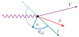
Figure 6: (Color online) Geometry of reaction (1).

It is worth noting that $\mathbf{l}$ and $\mathbf{p}_{p}$ are not fixed, but are themselves functions of $\theta_{nl}$. Both the direction and magnitude of $\mathbf{l}$ change, and since $\mathbf{l}=\mathbf{p}_{p}+\mathbf{p}_{n}$, as $\theta_{nl}$ gets larger, so does $\theta_{pl}$.

One expects rescattering peaks to occur where the fast scattered hadron is roughly transverse with the scatterer. As can be seen in Fig. 6, this will occur for fairly small $\theta_{nl}$ for the $V$-$n$ rescattering peak, but for larger $\theta_{nl}$ for the $p$-$n$ rescattering peak. Thus, we expect as a general rule, $\theta_{nl}^{pn}>\theta_{nl}^{VN}$, where the superscript indicates that this angle is where a rescattering peak occurs.

IV.2 Photoproduction of $\phi$ mesons

Recent studies of $\phi$ meson photoproduction from nuclei have generated much interest due to a large $\phi$-$N$ cross-section observed at near-threshold energiesIshikawa et al. (2005); Wood et al. (2010). The $\phi$-$N$ cross-sections are usually extracted by studying the $A$ dependence of the differential cross-section and employing a Glauber-like analysis. The extracted results vary from $20$ to $70~{}\mathrm{mb}$Qian et al. (2011), significantly exceeding the vector meson dominance prediction of $10~{}\mathrm{mb}$.

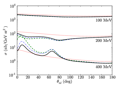
Figure 7: (Color online) Angular dependence of the $\phi$ photoproduction cross-section at different neutron momenta, assuming $\sigma_{\phi N}=30~{}\mathrm{mb}$ and $B=10~{}\mathrm{GeV}^{-2}$. The dotted (red) line indicates PWIA. Dashed (green) indicates PWIA and the first two single rescattering terms (off-neutron production is neglected). Dash-dotted (blue) indicates PWIA + all single rescattering. Solid (black) indicates PWIA, single, and double rescattering. $q_{0}=5~{}\mathrm{GeV}$ and $-t=1.2~{}\mathrm{GeV}^{2}$.

A deuteron target was used in several recent experimentsMibe et al. (2007); Qian et al. (2009, 2011). In Ref. Qian et al. (2009), the analysis of the $d(\gamma,pK^{+}K^{-})n$ exclusive reaction for photon energies in the range $1.65-3.59~{}\mathrm{GeV}$ yielded a $\phi$-$N$ cross-section above $20~{}\mathrm{mb}$. While measurements of the coherent reaction $d(\gamma,\phi)d$ clearly indicate the presence of $\phi$-$N$ rescattering, they could not distinguish between the vector meson dominance value of $\sigma_{\phi N}=10~{}\mathrm{mb}$ and the recently measured $\sigma_{\phi N}=30~{}\mathrm{mb}$, provided the slope factor is assumed to be around $10~{}\mathrm{GeV}^{-2}$Mibe et al. (2007).

To demonstrate the sensitivity of the break-up reaction to the $\phi$-$N$ scattering parameters, we performed numerical evaluations of the cross-section (39) at energies for which a coherent $\phi$ production experiment was performed at JLabMibe et al. (2007).

In Fig. 7, we present the angular distribution of the cross-section at different values of the recoil neutron momentum, calculated assuming $\sigma_{\phi N}=30~{}\mathrm{mb}$ and $B=10~{}\mathrm{GeV}^{-2}$. The cross-section value of $30~{}\mathrm{mb}$ is suggested by recent experiments (cf. Ishikawa et al. (2005); Wood et al. (2010)) and the value of the slope factor by an analysis in Ref. Mibe et al. (2007). Here we use the shorthand notation

$$\sigma\equiv\frac{d^{5}\sigma}{dp_{V}d\Omega_{V}d\Omega_{p}}.$$ (42)

The figure shows an angular distribution qualitatively similar to what is observed in $d(e,e^{\prime}p)n$ reactionsSargsian (2010); Egiyan et al. (2007); Boeglin et al. (2011): for neutron momenta $\leq 200~{}\mathrm{MeV}$ screening effects are dominant, as FSIs decrease the overall cross-section due to destructive interference between the PWIA amplitude $\mathcal{M}_{0}$ and the single rescattering amplitude $\mathcal{M}_{1}=\mathcal{M}_{1a}+\mathcal{M}_{1b}$. For $p_{n}\geq 400~{}\mathrm{MeV}$ the cross-section is dominated by the square of single rescattering amplitude, which results in an increase in the cross-section as compared to the PWIA value. The present case differs from the $d(e,e^{\prime}p)n$ reaction, however, in that two distinct screening minima are observed for $p_{n}=200~{}\mathrm{MeV}$, due to the presence of both a $\phi$-$N$ and a $p$-$n$ rescattering. Likewise, two distinct peaks can be seen for $p_{n}=400~{}\mathrm{MeV}$: a $\phi$-$N$ rescattering peak at $\theta_{nl}=8^{\circ}$ and a $p$-$n$ rescattering peak at $\theta_{nl}=65^{\circ}$, in agreement with the discussion of Sec. IV.1 (cf. as well Fig. 6).

One new feature of the angular distributions in Fig. 7 is the presence of a rescattering amplitude $\mathcal{M}_{1c}$ which corresponds to production of the $\phi$ meson from the neutron, which partially cancels the overall effect of the other FSIs since it enters with a negative sign relative to $\mathcal{M}_{1a}$ and $\mathcal{M}_{1b}$. This negative sign is due to antisymmetry of the deuteron wave-function under a $p\leftrightarrow n$ transposition.

The presence of either screening or peaks at different recoil neutron momenta suggests the ratio

$$R=\frac{\sigma(p_{n}=400~{}\mathrm{MeV})}{\sigma(p_{n}=200~{}\mathrm{MeV})}$$ (43)

as especially conducive to our study, as the valleys in the angular distribution for $p_{n}=200~{}\mathrm{MeV}$ entering into the denominator of $R$ will enhance the peaks entering into the numerator.

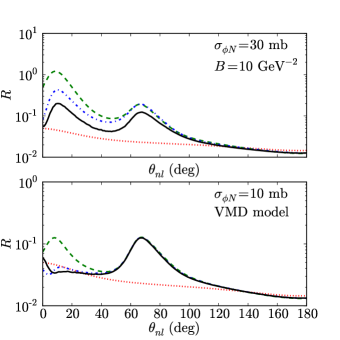
Figure 8: (Color online) Angular dependence of the ratio defined in Eq. (43), for two models of the $\phi$-$N$ interaction. Lines have the same meaning as in Fig. 7. $q_{0}=5~{}\mathrm{GeV}$ and $-t=1.2~{}\mathrm{GeV}^{2}$.

In Fig. 8 we present predictions for the ratio (43) for two models of $\phi$-$N$ scattering. In the upper panel, we use $\sigma_{\phi N}=30~{}\mathrm{mb}$ and $B_{\phi N}=10~{}\mathrm{GeV}^{-2}$ (the same parameterization as in Fig. 7), while in the lower panel we use $\sigma_{\phi N}=10~{}\mathrm{mb}$ and assume vector meson dominance, so $\phi$-$N$ scattering has the same $t$ dependence as photoproduction. In both cases we use $\alpha=-0.5$. As the figures show, the two models predict significantly different ratios for the $\phi$-$N$ cross-section. Qualitatively, no $\phi$-$N$ rescattering peak is seen for the $\sigma_{\phi N}=10~{}\mathrm{mb}$ model, as $\mathcal{M}_{1a}$ and $\mathcal{M}_{1c}$ almost completely cancel. Quantitatively, the magnitudes of $R$ for the two models differ by almost an order of magnitude at the $\phi$-$N$ rescattering peak. Thus these estimates indicate that the break-up reaction (1) is able to effectively discriminate between different models of $\phi$-$N$ scattering, and can complement other methods of studying the $\phi$-$N$ interaction.

IV.3 Photoproduction of $J/\Psi$ Mesons

In studying the photoproduction of $J/\Psi$ in reaction (1), we focus on several aspects of the eikonal dynamics of the FSIs. Namely, for the near-threshold kinematics we will concentrate on identifying the $J/\Psi$-$N$ rescattering peak in the angular distribution as we did in the case of $\phi$. For below-threshold production we will elaborate the kinematic requirements of photoproduction, which result in a strong suppression of FSI effects. Finally, for $J/\Psi$ production at collider energies, we demonstrate almost complete cancelation of the $J/\Psi$-$N$ rescattering due to destructive interference between single rescattering amplitudes.

IV.3.1 Near-threshold Photoproduction of $J/\Psi$ Mesons

The upcoming $12~{}\mathrm{GeV}$ upgrade at Jefferson LabDudek et al. (2012) will cross the $J/\Psi$ photoproduction threshold for a proton target. This will provide unprecedented opportunities for studies of $J/\Psi$ photoproduction at near-threshold kinematics, for which there are currently very limited data (see e.g. Refs. Gittelman et al. (1975); Camerini et al. (1975)).

This has renewed interest in theoretical studies of the $J/\Psi$-$N$ interaction at near-threshold kinematics through photo- and electroproduction from the deuteronHowell and Miller (2013); Wu and Lee (2013). The present analysis is focused on studying the sensitivity of the reaction (1) to the cross-section of the $J/\Psi$-$N$ interaction through ratios similar to that of Eq. (43).

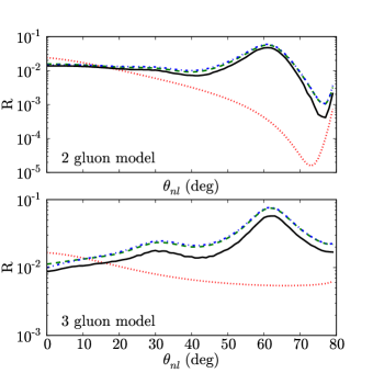
Figure 9: (Color online) Angular dependence of the ratio defined in Eq. (44), for the two- and three-gluon exchange models of $J/\Psi$ photoproduction. Assumes $\sigma_{\Psi N}=5~{}\mathrm{mb}$. Lines have the same meaning as in Fig. 7. $q_{0}=10~{}\mathrm{GeV}$ and $t=t_{\mathrm{thr.}}=-2.23~{}\mathrm{GeV}^{2}$.

The $J/\Psi$-nucleon interaction near threshold is not well understood. At high energies, vector meson dominance suggests a total cross-section of around $1~{}\mathrm{mb}$Knapp et al. (1975), while experimental data indicates a higher value of $3.5~{}\mathrm{mb}$Anderson et al. (1977). On the theoretical side, the two-gluon exchange models suggest a monotonically increasing total cross-section that approaches an asymptotic value at large energiesKharzeev and Satz (1994), and accordingly a smaller cross-section near threshold. While these models are based on a leading twist approximation, other models that attempt to account for nonperturbative effects suggest a significantly larger cross section, as large as $17~{}\mathrm{mb}$ near thresholdSibirtsev and Voloshin (2005).

To ascertain the sensitivity of the considered break-up reaction to the $J/\Psi$-$N$ cross-section, we consider the ratio

$$R=\frac{\sigma(p_{n}=600~{}\mathrm{MeV})}{\sigma(p_{n}=200~{}\mathrm{MeV})},$$ (44)

where for the numerator we choose the cross section at larger value of recoil nucleon momenta to maximize the rescattering effects, and thereby the sensitivity of the $R$ to the $J/\Psi$-$N$ scattering amplitude.

Since the $J/\Psi$ photoproduction amplitude is not factorized from the FSI amplitudes, care should be given to the treatment of the $\gamma N\rightarrow J/\Psi N$ amplitude, which can be strongly energy-dependent at near-threshold kinematics. For this reason we consider two alternative models for $J/\Psi$ photoproduction near the threshold. In the first model, the energy dependence of the photoproduction amplitude is estimated based on the leading-twist two-gluon exchange modelBrodsky et al. (2001), according to which the function $A(s)$ entering into Eq. (41) can be parameterized as

$$A_{2g}(s)=\frac{\mathcal{N}_{2g}}{\sqrt{1+\alpha^{2}}}\left(\frac{s-s_{\mathrm{thr.},N}}{s-m_{N}^{2}}\right),$$ (45)

with the constant $\mathcal{N}_{2g}=1.38~{}\mathrm{GeV}^{-2}$ found from a fit to photoproduction dataCamerini et al. (1975). The slope factor $B$ is estimated from the two-gluon form factor of the nucleon asFrankfurt and Strikman (2002)

$$B_{\mathrm{eff.}}=\frac{4}{1~{}\mathrm{GeV}^{2}-t}.$$ (46)

It is worth noting that at $t=-2.23~{}\mathrm{GeV}^{2}$, $B_{\mathrm{eff.}}\approx 1.24~{}\mathrm{GeV}^{-2}$, which is close to the low-energy $B$ value of $1.25~{}\mathrm{GeV}^{-2}$ measured at a Cornell experimentGittelman et al. (1975).

The observation that the very limited phase space near threshold may favor a coherent interaction of all three quarks in the nucleon suggests the possible dominance of a three-gluon exchange mechanism, which predicts much weaker energy dependence at the thresholdBrodsky et al. (2001):

$$A_{3g}(s)=\frac{\mathcal{N}_{3g}}{\sqrt{1+\alpha^{2}}},$$ (47)

with the constant $\mathcal{N}_{3g}=0.36~{}\mathrm{GeV}^{-2}$ fit to the results of Ref. Gittelman et al. (1975). For this model, we adopted a constant slope factor $B=1.25~{}GeV^{-2}$, consistent with experimental dataGittelman et al. (1975). In both cases, we use $\alpha=-0.2$.

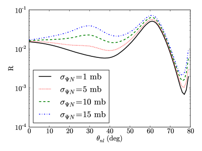
Figure 10: (Color online) Angular dependence of the ratio defined in Eq. (44) with different $J/\Psi$-$N$ cross-sections, using the two-gluon parameterization of Brodsky et al. (2001). Estimated at $p_{n}=400~{}\mathrm{MeV}$, $q_{0}=10~{}\mathrm{GeV}$ and $-t=2.23~{}\mathrm{GeV}^{2}$. Includes all diagrams.

In Fig. 9 we present the prediction of above models, where the diffractive part of the $J\Psi$-$N$ amplitude is parameterized with $\sigma_{\Psi N}=5~{}\mathrm{mb}$ and $B=1.25~{}\mathrm{GeV}^{-2}$. This figure indicates the presence of two rescattering peaks, with the peak at $\theta_{nl}=30^{\circ}$ corresponding to $J/\Psi$-$N$ rescattering. This pattern of two rescattering peaks, each corresponding to one of the rescattering diagrams, has also been observed in Ref. Howell and Miller (2013).

These estimates also demonstrate the sensitivity of the reaction (1) to the energy dependence of the photoproduction amplitude. For the two-gluon mechanism, a dip should be present near the kinematical limit of $\theta_{nl}$ due to the threshold factor of $s-s^{0}_{\mathrm{thr.},N}$. At this $\theta_{nl}$, the angle between the outgoing proton and the $J/\Psi$ meson becomes smaller, thus making $s_{\gamma p}=m_{N}^{2}+m_{\Psi}^{2}+2E_{p}E_{\Psi}-2\mathbf{p}_{p}\cdot\mathbf{p}_{\Psi}$ smaller as well. No such suppression factor exists for the three-gluon model. Besides this, Fig. 9 demonstrates that the effect of $\mathcal{M}_{1c}$ is negligible, owing to the large value of $-t_{\mathrm{thr.}}$.

We conclude our discussion of near-threshold $J/\Psi$ production from the deuteron by presenting, in Fig. 10, estimates of $R$ (see Eq. 44) for the two-gluon exchange model of Eq. (45) for several values of $\sigma_{\Psi N}$, thus demonstrating the sensitivity of reaction (1) to the total $J/\Psi$-$N$ cross-section.

IV.3.2 Sub-threshold Photoproduction of $J/\Psi$ Mesons

While the threshold for $J/\Psi$ photoproduction from a stationary proton is $E_{\mathrm{thr.},N}=8.2~{}\mathrm{GeV}$, the threshold for production from the deuteron is only $5.6~{}\mathrm{GeV}$, making it kinematically possible to produce $J/\Psi$ with $q_{0}<E_{\mathrm{thr.},N}$. This requires that the bound nucleon struck by the photon be sufficiently fast so that $s_{\gamma N}\geq s_{\mathrm{thr.},N}=(m_{n}+m_{\Psi})^{2}$. The kinematics of reaction (1) allow for this when the recoil neutron flies off in the forward direction. Within PWIA this will correspond to the $J/\Psi$ meson off a backward moving proton that satisfy the condition

$$(q+p_{p}^{\prime})^{2}>s_{\mathrm{thr.},N}.$$ (48)

This condition can only be satisfied for fast, backwards-going protons that satisfy the condition

$$|\mathbf{p}_{p}^{\prime}|\geq p_{\mathrm{thr.}}(q_{0},\theta_{p}^{\prime}),$$ (49)

where $\theta_{p}^{\prime}$ is the angle between the bound proton and the photon. This threshold momentum is shown as a function of $q_{0}$ in Fig. 11 for several values of $\theta_{p}^{\prime}$. The value of $p_{\mathrm{thr.}}$ can be very large for small photon energies, even above $700~{}\mathrm{MeV}$. At these photon energies, we expect the applicability of VNA to break down, so its predictions will be rather qualitative. However, key features such as the onset of the eikonal regime for rescattering will be relevant to other (e.g. light cone) approximations which are better suited to describing sub-threshold production.

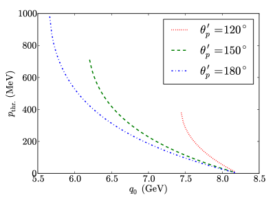
Figure 11: (Color online) The threshold value for $J/\Psi$ photoproduction of the bound proton momentum as a function of photon energy for various proton-photon angles.

As for FSIs, we may expect immediately that $\mathcal{M}_{1c}$ does not contribute, since $-t_{\mathrm{thr.}}$ is large and $q_{0}$ is small. As for $\mathcal{M}_{1a}$ and $\mathcal{M}_{1b}$, one of the analytic properties of their pole parts (Eqs. (19,22)) is that

$$p_{n,z}=p_{n,z}^{\prime}+\Delta_{1a/1b}$$ (50)

which, because of momentum conservation at the $d\rightarrow pn$ vertex, implies

$$p_{n,z}=-p_{p,z}^{\prime}+\Delta_{1a/ab/1c}=-|\mathbf{p}_{p}^{\prime}|\cos(\theta_{p}^{\prime})+\Delta_{1a/1b}.$$ (51)

As can be seen in Eqs. (17,21), the factors $\Delta_{1a}$ and $\Delta_{1b}$ are both positive. This means that $p_{n,z}>-|\mathbf{p}_{p}^{\prime}|\cos(\theta_{p}^{\prime})$, with the lesser quantity a positive number since the struck proton will be backwards-going. To be compatible with the inequality (49), this requires an especially large $p_{n,z}$. However, the $\Delta$ factors monotonically increase with $p_{n,z}$, making the condition (51) more difficult to fulfill. Thus, we expect a suppression of FSIs for sub-threshold kinematics. This is illustrated in Fig. 12, where we present numerical estimates for the $J/\Psi$ production cross-section at $q_{0}=7~{}\mathrm{GeV}$ using the two- and three-gluon exchange models of Ref. Brodsky et al. (2001). As the figure shows, the FSI effects are small and, contrary to above threshold kinematics, do not increase with increased $p_{n}$. Looking back at Fig. 11, we conclude that at sub-threshold kinematics the reaction (1) in the limit $q_{0}\rightarrow E_{\mathrm{thr.}}^{\mathrm{deut.}}$ will allow probing of the internal structure of the deuteron at large Fermi momenta with little distortion from FSIs.

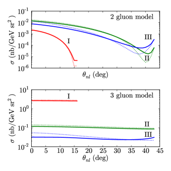
Figure 12: (Color online) Angular dependence of the $J/\Psi$ photoproduction cross-section at different neutron momenta below threshold. Assumes $\sigma_{\Psi N}=5~{}\mathrm{mb}$. The curves I, II, and III represent $p_{n}$ equal to $200$, $400$, and $600$ MeV, respectively. The dotted and solid lines are PWIA and full calculations, respectively. $q_{0}=7~{}\mathrm{GeV}$ and $t=t_{\mathrm{thr.},N}=-2.23~{}\mathrm{GeV}^{2}$.

IV.4 Photoproduction of $J/\Psi$ at Collider Energies

As was mentioned in Sec. III.2, due to antisymmetry of deuteron wave-function, the $J/\Psi$-$N$ rescatteirng amplitude of Fig. 4(c) enters with the opposite sign relative to the other $J/\Psi$-$N$ rescattering amplitude of Fig. 4(a). It was observed in Sec. IV.3 that the contribution of $\mathcal{M}_{1c}$ will be small for near-threshold kinematics, so there is little cancelation with the contribution of $\mathcal{M}_{1a}$. This was due to the large value of $t_{\mathrm{min.}}\sim t_{\mathrm{thr.}}$, which required both vertices in Fig. 4(c) to be hard.

However, for large photon energies, $t_{\mathrm{min.}}\rightarrow 0$ and thus we expect almost complete cancelation between $\mathcal{M}_{1a}$ and $\mathcal{M}_{1c}$. This represents a situation where the $J/\Psi$ meson will not participate in FSIs.

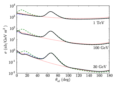
Figure 13: (Color online) Angular dependence of the $J/\Psi$ photoproduction cross-section at collider energies, given $t=-1.5~{}\mathrm{GeV}^{2}$ and $p_{n}=400~{}\mathrm{MeV}$. Assumes $\sigma_{\Psi N}=5~{}\mathrm{mb}$. Lines have the same meaning as in Fig. 7.

To estimate the cancelation effect numerically, we calculated the cross-section of the reaction (1) for collider energies. We parameterize the $s$ dependence of the $\gamma N\rightarrow J/\Psi N$ amplitude using a leading-order pQCD approximationRebyakova et al. (2012). In particular, for the function $A(s)$ entering into Eq. (41), we use

$$A(s)=\mathcal{N}\alpha_{s}(\mu^{2})xG_{T}(x,\mu^{2}),$$ (52)

where $G_{T}(x,\mu^{2})$ is the gluonic distribution of the target nucleon at factorization scale $\mu^{2}$. Here $x=\frac{m_{\Psi}^{2}}{s_{\gamma N^{*}}}$, and we choose $\mu^{2}=\frac{m_{\Psi}^{2}}{4}$ similar to Rebyakova et al. (2012). For these estimates we used the CJ12 next-to-leading order partonic distribution functionsOwens et al. (2012), and we modeled the $t$ dependence using a slope factor of $B=4.73~{}\mathrm{GeV}^{-2}$Adloff et al. (2000).

The results for three photon beam energies (with a recoil neutron momentum of $400~{}\mathrm{MeV}$) are given in Fig. 13. They demonstrate significant cancelation of the two $J/\Psi$-$N$ rescattering amplitudes, with the cancelation becoming predominant with increasing photon energy. Even for $q_{0}=30~{}\mathrm{GeV}$ the FSI effects at $\theta_{nl}\approx 30^{\circ}$ (where one expects maximal $J/\Psi$-$N$ rescattering) contribute less than a few percent of the total cross-section. The overall FSI effects are due only to $p$-$n$ reinteractions.

It is worth noting that the observed cancelation is also valid for other nuclei, since it is due to the antisymmetry of the nuclear wave-function. Thus the present result suggests that $J/\Psi$ mesons produced from nuclei in coincidence with a knock-out nucleon will not undergo first order $J/\Psi$-$N$ rescattering, which may significantly reduce their absorption.

V Conclusions

With the virtual nucleon approximation, we calculated the large $-t\geq 1~{}\mathrm{GeV}^{2}$ cross-section for vector meson photoproduction from the deuteron accompanied by deuteron break-up. We focused on kinematics where one of the nucleons could be identified as struck and the other as a spectator to the $\gamma N\rightarrow VN$ subprocess. The large $-t$ involved validates the generalized eikonal approximation in calculating the final state interactions.

Our results indicate that, similarly to the $\gamma^{*}d\rightarrow pn$ reaction, one can observe a minimum or peak in the recoil nucleon angular distribution associated with a $p$-$n$ reinteraction. However, a novelty of the photoproduction reaction is that a second mininum or peak appears due to $V$-$N$ rescattering. Using $\phi(1020)$ and $J/\Psi$ as examples, we showed that this second peak (or minimum) can be used to probe characteristics of the largely unknown $V$-$N$ interaction. In the case of $J/\Psi$ in particular, we extended our calculations into the sub-threshold and high-energy domains.

The sub-threshold calculations demonstrated and overall suppression of final state interactions due to restrictive kinematical limitations. This result indicates that sub-threshold production can be used to probe the deuteron at extremely large internal momenta with little distortion due to FSIs.

In the high-energy limit, we observe a significant cancelation between $J/\Psi$-$N$ rescattering amplitudes associated with production from different nucleons in the deuteron. In this limit, FSI effects are due entirely to $p$-$n$ rescattering. This result suggests experiments where the $J/\Psi$ meson is detected in coincidence with a knocked out nucleon as a means of probing the $J/\Psi$ photoproduction with little contribution from $J/\Psi$-$N$ rescattering, as the cancelation strongly suppresses this contribution.

VI Acknowledgements

We are thankful to Drs. Gerald Miller, Mark Strikman, and Xin Qian for helpful comments and discussions. This work is supported by the U.S. Department of Energy grant under contract DE-FG02-01ER41172.

*

Appendix A Double Rescattering Term

Here we give the details of the derivation of the double scattering amplitudes presented in Sec. III.3. The derivation follows these steps of GEA:

1. The full amplitude is written out using the effective Feynman rules.

2. Energy integration places the spectator to photoproduction and a low-momentum internal nucleon on its mass shell.

3. Terms are gathered into the VNA deuteron wave-function.

4. A decomposition into pole and principal value parts is performed for each remaining propagator.

5. Completeness relations are used and terms gathered into subprocess (photoproduction and reinteraction) amplitudes.

All of the steps shall be here carried out in full detail for $\mathcal{M}_{2a}$, whereas a more cursory description shall be given for $\mathcal{M}_{2b}$ and $\mathcal{M}_{2c}$.

To begin, the full amplitude for the process in Fig. $\ref{fig:resc2}(a)$ is

$$\mathcal{M}_{2a}^{(\lambda_{V},\lambda_{p},\lambda_{n};\lambda_{\gamma},\lambda_{d})} =-\bar{u}^{(\lambda_{p})}(\mathbf{p}_{p})\bar{u}^{(\lambda_{n})}(\mathbf{p}_{n}){\phi^{*}_{\pi}}^{(\lambda_{V})}(\mathbf{p}_{V})\int\frac{d^{4}p_{n}^{\prime}}{(2\pi)^{4}i}\int\frac{d^{4}p_{n}^{\prime\prime}}{(2\pi)^{4}i}\bigg{[}\Gamma_{pn\rightarrow pn}\frac{\not{p}_{p}^{\prime\prime}+m_{N}}{(p_{p}^{\prime\prime})^{2}-m_{N}^{2}+i\epsilon}$$

$$\times\frac{\not{p}_{n}^{\prime\prime}+m_{N}}{(p_{n}^{\prime\prime})^{2}-m_{N}^{2}+i\epsilon}\Gamma^{\rho\pi}_{VN\rightarrow VN}\frac{G_{\rho\nu}(p_{V}^{\prime})}{(p_{V}^{\prime})^{2}-m_{V}^{2}+i\epsilon}\Gamma^{\mu\nu}_{\gamma N\rightarrow VN}\epsilon^{(\lambda_{\gamma})}_{\mu}(q)\frac{\not{p}_{p}^{\prime}+m_{N}}{(p_{p}^{\prime})^{2}-m_{N}^{2}+i\epsilon}$$

$$\times\frac{\not{p}_{n}^{\prime}+m_{N}}{(p_{n}^{\prime})^{2}-m_{N}^{2}+i\epsilon}\Gamma_{dpn}\chi^{(\lambda_{d})}\bigg{]},$$ (53)

where we have chosen the integration variable in anticipation of the positive-energy, on-shell projections that shall be executed. Firstly, as prescribed by VNA, a slow nucleon with momentum $p_{n}^{\prime}$ shall be placed on its mass shell. Of the remaining internal lines, $p_{n}^{\prime\prime}$ has the smallest momentum, since the photoproduction vertex is hard, giving the proton a large momentum, whereas the $V$-$N$ rescattering is soft. Doing these energy integrations and keeping the positive-energy parts, as well as using the exact completeness relations entailed by placing the neutron on-shell, gives

$$\mathcal{M}_{2a}^{(\lambda_{V},\lambda_{p},\lambda_{n};\lambda_{\gamma},\lambda_{d})} =-\bar{u}^{(\lambda_{p})}(\mathbf{p}_{p})\bar{u}^{(\lambda_{n})}(\mathbf{p}_{n}){\phi^{*}_{\pi}}^{(\lambda_{V})}(\mathbf{p}_{V})\sum_{\lambda_{n}^{\prime}\lambda_{n}^{\prime\prime}}\int\frac{d^{3}\mathbf{p}_{n}^{\prime}}{(2\pi)^{3}}\int\frac{d^{3}\mathbf{p}_{n}^{\prime\prime}}{(2\pi)^{3}}\bigg{[}\frac{1}{2E_{n}^{\prime}}\frac{1}{2E_{n}^{\prime\prime}}$$

$$\times\Gamma_{pn\rightarrow pn}u^{(\lambda_{n}^{\prime\prime})}(\mathbf{p}_{n}^{\prime\prime})\bar{u}^{(\lambda_{n}^{\prime\prime})}(\mathbf{p}_{n}^{\prime\prime})\frac{\not{p}_{p}^{\prime\prime}+m_{N}}{(p_{p}^{\prime\prime})^{2}-m_{N}^{2}+i\epsilon}\Gamma^{\rho\pi}_{VN\rightarrow VN}\frac{G_{\rho\nu}(p_{V}^{\prime})}{(p_{V}^{\prime})^{2}-m_{V}^{2}+i\epsilon}$$

$$\times u^{(\lambda_{n}^{\prime})}(\mathbf{p}_{n}^{\prime})\Gamma^{\mu\nu}_{\gamma N\rightarrow VN}\epsilon^{(\lambda_{\gamma})}_{\mu}(q)\frac{\not{p}_{p}^{\prime}+m_{N}}{(p_{p}^{\prime})^{2}-m_{N}^{2}+i\epsilon}\bar{u}^{(\lambda_{n}^{\prime})}(\mathbf{p}_{n}^{\prime})\Gamma_{dpn}\chi^{(\lambda_{d})}\bigg{]}.$$ (54)

Next, we use the approximate completeness relation $\not{p}_{p}^{\prime}+m_{N}\approx\sum_{\lambda_{p}^{\prime}}u^{(\lambda_{p}^{\prime})}(\mathbf{p}_{p}^{\prime})\bar{u}^{(\lambda_{p}^{\prime})}(\mathbf{p}_{p}^{\prime})$ for the virtual, struck proton so that we may gather terms into the deuteron wave-function defined in Eq. (6), as follows:

$$\mathcal{M}_{2a}^{(\lambda_{V},\lambda_{p},\lambda_{n};\lambda_{\gamma},\lambda_{d})} =-\bar{u}^{(\lambda_{p})}(\mathbf{p}_{p})\bar{u}^{(\lambda_{n})}(\mathbf{p}_{n}){\phi^{*}_{\pi}}^{(\lambda_{V})}(\mathbf{p}_{V})\sum_{\lambda_{p}^{\prime}\lambda_{n}^{\prime}\lambda_{n}^{\prime\prime}}\int\frac{d^{3}\mathbf{p}_{n}^{\prime}}{(2\pi)^{3}}\int\frac{d^{3}\mathbf{p}_{n}^{\prime\prime}}{(2\pi)^{3}}\bigg{[}\sqrt{\frac{2(2\pi)^{3}}{2E_{n}^{\prime}}}\frac{1}{2E_{n}^{\prime\prime}}$$

$$\times\Gamma_{pn\rightarrow pn}u^{(\lambda_{n}^{\prime\prime})}(\mathbf{p}_{n}^{\prime\prime})\bar{u}^{(\lambda_{n}^{\prime\prime})}(\mathbf{p}_{n}^{\prime\prime})\frac{\not{p}_{p}^{\prime\prime}+m_{N}}{(p_{p}^{\prime\prime})^{2}-m_{N}^{2}+i\epsilon}\Gamma^{\rho\pi}_{VN\rightarrow VN}\frac{G_{\rho\nu}(p_{V}^{\prime})}{(p_{V}^{\prime})^{2}-m_{V}^{2}+i\epsilon}$$

$$\times u^{(\lambda_{n}^{\prime})}(\mathbf{p}_{n}^{\prime})\Gamma^{\mu\nu}_{\gamma N\rightarrow VN}\epsilon^{(\lambda_{\gamma})}_{\mu}(q)u^{(\lambda_{p}^{\prime})}(\mathbf{p}_{p}^{\prime})\Psi_{d}^{(\lambda_{p}^{\prime},\lambda_{n}^{\prime};\lambda_{d})}(\mathbf{p}_{n}^{\prime})\bigg{]}.$$ (55)

From here, we change the integration variables to the transferred momentum at each vertex, namely

$$K =p_{n}-p_{n}^{\prime\prime}$$ (56)

$$K^{\prime} =p_{n}^{\prime\prime}-p_{n}^{\prime}$$ (57)

and write the remaining propagators in terms of these momenta. For the proton propagator,

$$(p_{p}^{\prime\prime})^{2}-m_{N}^{2}+i\epsilon =(p_{p}+p_{n}-p_{n}^{\prime\prime})^{2}-m_{N}^{2}+i\epsilon=(p_{p}+K)^{2}-m_{N}^{2}+i\epsilon$$

$$=K^{2}+2E_{p}K_{0}-\mathbf{p}_{p}\cdot\mathbf{K}_{\perp}-p_{p,z}K_{z}+i\epsilon$$

$$=2p_{p,z}(\Delta_{2a}-K_{z}+i\epsilon),$$ (58)

where

$$\Delta_{2a}=\frac{K^{2}+2E_{p}K_{0}-2\mathbf{p}_{p}\cdot\mathbf{K}_{\perp}}{2p_{p,z}}$$ (59)

and for the vector meson propagator

$$(p_{V}^{\prime})^{2}-m_{V}^{2}+i\epsilon =(p_{V}+p_{n}^{\prime\prime}-p_{n}^{\prime})^{2}-m_{V}^{2}+i\epsilon=(p_{V}+K^{\prime})^{2}-m_{V}^{2}+i\epsilon$$

$$=(K^{\prime})^{2}+2E_{V}K^{\prime}_{0}-\mathbf{p}_{V}\cdot\mathbf{K}^{\prime}_{\perp}-p_{V,z}K^{\prime}_{z}+i\epsilon$$

$$=2p_{V,z}(\Delta^{\prime}_{2a}-K^{\prime}_{z}+i\epsilon),$$ (60)

where

$$\Delta^{\prime}_{2a}=\frac{(K^{\prime})^{2}+2E_{V}K^{\prime}_{0}-2\mathbf{p}_{V}\cdot\mathbf{K}^{\prime}_{\perp}}{2p_{V,z}}.$$ (61)

With the propagator denominators in this form, we can decompose the integrals over each of $K_{z}$ and $K^{\prime}_{z}$ into pole and principal value parts. Because the principal value part will be small compared to the pole part, and because double rescattering will itself be small compared to single rescattering, we consider only the pole parts of each integral, placing both the proton and vector meson on their mass shells. This allows us to use completeness relations for both, giving

$$\mathcal{M}_{2a}^{(\lambda_{V},\lambda_{p},\lambda_{n};\lambda_{\gamma},\lambda_{d})} =-\frac{1}{4p_{p,z}p_{V,z}}\sum_{\lambda_{p}^{\prime}\lambda_{n}^{\prime}\lambda_{p}^{\prime\prime}\lambda_{n}^{\prime\prime}\lambda_{V}^{\prime}}\int\frac{d^{2}\mathbf{K}_{\perp}}{(2\pi)^{2}}\int\frac{d^{2}\mathbf{K}^{\prime}_{\perp}}{(2\pi)^{2}}\bigg{[}\sqrt{\frac{2(2\pi)^{3}}{2E_{n}^{\prime}}}\frac{1}{2E_{n}^{\prime\prime}}$$

$$\times\bar{u}^{(\lambda_{p})}(\mathbf{p}_{p})\bar{u}^{(\lambda_{n})}(\mathbf{p}_{n})\Gamma_{pn\rightarrow pn}u^{(\lambda_{n}^{\prime\prime})}(\mathbf{p}_{n}^{\prime\prime})u^{(\lambda_{p}^{\prime\prime})}(\mathbf{p}_{p}^{\prime\prime})$$

$$\times\bar{u}^{(\lambda_{n}^{\prime\prime})}(\mathbf{p}_{n}^{\prime\prime}){\phi^{*}_{\pi}}^{(\lambda_{V})}(\mathbf{p}_{V})\Gamma^{\rho\pi}_{VN\rightarrow VN}{\phi^{*}_{\nu}}^{(\lambda_{V}^{\prime})}(\mathbf{p}_{V}^{\prime})u^{(\lambda_{n}^{\prime})}(\mathbf{p}_{n}^{\prime})$$

$$\times\bar{u}^{(\lambda_{p}^{\prime\prime})}(\mathbf{p}_{p}^{\prime\prime})\phi^{(\lambda_{V}^{\prime})}_{\rho}(\mathbf{p}_{V}^{\prime})\Gamma^{\mu\nu}_{\gamma N\rightarrow VN}\epsilon^{(\lambda_{\gamma})}_{\mu}(q)u^{(\lambda_{p}^{\prime})}(\mathbf{p}_{p}^{\prime})$$

$$\times\Psi_{d}^{(\lambda_{p}^{\prime},\lambda_{n}^{\prime};\lambda_{d})}(p_{n,z}-\Delta_{2a}-\Delta_{2a}^{\prime};\mathbf{p}_{n,\perp}-\mathbf{K}_{\perp}-\mathbf{K}^{\prime}_{\perp})\bigg{]}.$$ (62)

Terms are then gathered into subprocess (photoproduction and rescattering) amplitudes, giving

$$\mathcal{M}_{2a}^{(\lambda_{V},\lambda_{p},\lambda_{n};\lambda_{\gamma},\lambda_{d})} =-\frac{1}{4p_{p,z}p_{V,z}}\sum_{\mathrm{spins}}\int\frac{d^{2}\mathbf{K}}{(2\pi)^{2}}\int\frac{d^{2}\mathbf{K}^{\prime}}{(2\pi)^{2}}\bigg{[}\sqrt{\frac{2(2\pi)^{3}}{2E_{n}^{\prime}}}\frac{1}{2E_{n}^{\prime\prime}}\mathcal{M}_{pn\rightarrow pn}^{(\lambda_{p},\lambda_{n};\lambda_{p}^{\prime\prime},\lambda_{n}^{\prime\prime})}(p_{p},p_{n};p_{p}^{\prime\prime},p_{n}^{\prime\prime})$$

$$\times\mathcal{M}_{VN\rightarrow VN}^{(\lambda_{V},\lambda_{n}^{\prime\prime};\lambda_{V}^{\prime},\lambda_{n}^{\prime})}(p_{V},p_{n}^{\prime\prime};p_{V}^{\prime},p_{n}^{\prime})\mathcal{M}_{\gamma N\rightarrow VN}^{(\lambda_{V}^{\prime},\lambda_{p}^{\prime\prime};\lambda_{\gamma},\lambda_{p}^{\prime})}(p_{V}^{\prime},p_{p}^{\prime\prime};p_{\gamma},p_{p}^{\prime})$$

$$\times\Psi_{d}^{(\lambda_{p}^{\prime},\lambda_{n}^{\prime};\lambda_{d})}(p_{n,z}-\Delta_{2a}-\Delta_{2a}^{\prime};\mathbf{p}_{n,\perp}-\mathbf{K}_{\perp}-\mathbf{K}^{\prime}_{\perp})\bigg{]},$$ (63)

where the sum is over all internal spins. This is exactly Eq. (29).

The same process is followed for calculating $\mathcal{M}_{2b}$ and $\mathcal{M}_{2c}$, but with a few minor differences. First, regarding $\mathcal{M}_{2b}$. The momentum line $p_{n}^{\prime}$ corresponds to the spectator, so it is to be taken on-shell via energy integration. Of the remaining momentum lines, $p_{n}^{\prime\prime}$ is slow, so it too is placed on-shell by energy integration. The propagator for $p_{p}^{\prime}$ is absorbed into the deuteron wave-function, so the remaining propagators are for $p_{p}^{\prime\prime}$ and $p_{V}^{\prime}$. Momentum conservation, as before, can be used to rewrite the propagators in terms of the transferred momenta $K=p_{n}-p_{n}^{\prime\prime}$ and $K^{\prime}=p_{n}^{\prime\prime}-p_{n}^{\prime}$ and to find what the delta factors are. In particular,

$$(p_{V}^{\prime})^{2}-m_{V}^{2}+i\epsilon =(p_{V}+p_{n}-p_{n}^{\prime\prime})^{2}-m_{V}^{2}+i\epsilon=(p_{V}+K)^{2}-m_{V}^{2}+i\epsilon$$

$$=K^{2}+2E_{V}K_{0}-\mathbf{p}_{V}\cdot\mathbf{K}_{\perp}-p_{V,z}K_{z}+i\epsilon$$

$$=2p_{V,z}(\Delta_{2a}-K_{z}+i\epsilon)$$ (64)

$$(p_{p}^{\prime\prime})^{2}-m_{N}^{2}+i\epsilon =(p_{p}+p_{n}^{\prime\prime}-p_{n}^{\prime})^{2}-m_{N}^{2}+i\epsilon=(p_{p}+K^{\prime})^{2}-m_{N}^{2}+i\epsilon$$

$$=(K^{\prime})^{2}+2E_{p}K^{\prime}_{0}-\mathbf{p}_{p}\cdot\mathbf{K}^{\prime}_{\perp}-p_{p,z}K^{\prime}_{z}+i\epsilon$$

$$=2p_{p,z}(\Delta^{\prime}_{2b}-K^{\prime}_{z}+i\epsilon),$$ (65)

where

$$\Delta_{2b} =\frac{K^{2}+2E_{V}K_{0}-2\mathbf{p}_{V}\cdot\mathbf{K}_{\perp}}{2p_{V,z}}$$ (66)

$$\Delta^{\prime}_{2b} =\frac{(K^{\prime})^{2}+2E_{p}K^{\prime}_{0}-2\mathbf{p}_{p}\cdot\mathbf{K}^{\prime}_{\perp}}{2p_{p,z}}.$$ (67)

Next, regarding $\mathcal{M}_{2c}$. The momentum line $p_{p}^{\prime}$ is the spectator to photoproduction, so it is placed on-shell by energy integration. The $V$-$N$ rescattering vertex is hard, so $p_{p}^{\prime\prime}$ is fast, whereas the photoproduction vertex is soft, making $p_{n}^{\prime\prime}$ slow. Thus, it is $p_{n}^{\prime\prime}$ that will also be put on its mass shell. The propagator for $p_{n}^{\prime}$ is absorbed into the deuteron wave-function, so the remaining propgators are those for $p_{V}^{\prime}$ and $p_{p}^{\prime\prime}$. By momentum conservation, we rewrite them in the following forms and find the delta factors:

$$(p_{p}^{\prime\prime})^{2}-m_{N}^{2}+i\epsilon =(p_{p}+p_{n}-p_{n}^{\prime\prime})^{2}-m_{N}^{2}+i\epsilon=(p_{p}+K)^{2}-m_{N}^{2}+i\epsilon$$

$$=K^{2}+2E_{p}K_{0}-\mathbf{p}_{p}\cdot\mathbf{K}_{\perp}-p_{p,z}K_{z}+i\epsilon$$

$$=2p_{p,z}(\Delta_{2c}-K_{z}+i\epsilon)$$ (68)

$$(p_{V}^{\prime})^{2}-m_{V}^{2}+i\epsilon =(q+p_{n}^{\prime\prime}-p_{n}^{\prime})^{2}-m_{V}^{2}+i\epsilon=(q-K^{\prime})^{2}-m_{V}^{2}+i\epsilon$$

$$=(K^{\prime})^{2}-2q_{0}K^{\prime}_{0}-q_{0}K^{\prime}_{z}+i\epsilon$$

$$=2q_{0}(K^{\prime}_{z}-\Delta^{\prime}_{2c}+i\epsilon),$$ (69)

where

$$\Delta_{2c} =\frac{K^{2}+2E_{p}K_{0}-2\mathbf{p}_{p}\cdot\mathbf{K}_{\perp}}{2p_{p,z}}$$ (70)

$$\Delta^{\prime}_{2c} =\frac{(K^{\prime})^{2}-m_{V}^{2}}{2q_{0}}+K^{\prime}_{0}.$$ (71)

After this procedure is done for $\mathcal{M}_{2b}$ and $\mathcal{M}_{2c}$, the pole term in each integral is kept, completeness relations are used, and terms are gathered into subprocess amplitudes, resulting in Eqs. (30) and (31).

References

- (1) T. Bauer, R. Spital, D. Yennie, and F. Pipkin, Rev. Mod. Phys. 50, 261.
- Glauber and Matthiae (1970) R. Glauber and G. Matthiae, Nucl. Phys. B21, 135 (1970).
- Anderson et al. (1971) R. L. Anderson, D. Gustavson, J. Johnson, I. Overman, D. Ritson, et al., Phys. Rev. D4, 3245 (1971).
- Frankfurt et al. (1997a) L. Frankfurt, W. Koepf, J. Mutzbauer, G. Piller, M. Sargsian, et al., Nucl. Phys. A622, 511 (1997a), arXiv:hep-ph/9703399 [hep-ph] .
- Rogers et al. (2006) T. Rogers, M. Sargsian, and M. Strikman, Phys. Rev. C73, 045202 (2006), arXiv:hep-ph/0509101 [hep-ph] .
- Mibe et al. (2007) T. Mibe et al. (CLAS Collaboration), Phys. Rev. C76, 052202 (2007), arXiv:nucl-ex/0703013 [NUCL-EX] .
- Frankfurt et al. (1995a) L. Frankfurt, W. Greenberg, G. Miller, M. Sargsian, and M. Strikman, Z.Phys. A352, 97 (1995a), arXiv:nucl-th/9501009 [nucl-th] .
- Frankfurt et al. (1997b) L. Frankfurt, M. Sargsian, and M. Strikman, Phys. Rev. C56, 1124 (1997b), arXiv:nucl-th/9603018 [nucl-th] .
- Sargsian (2001) M. M. Sargsian, Int. J. Mod. Phys. E10, 405 (2001), arXiv:nucl-th/0110053 [nucl-th] .
- Ciofi degli Atti and Kaptari (2005) C. Ciofi degli Atti and L. Kaptari, Phys. Rev. C71, 024005 (2005), arXiv:nucl-th/0407024 [nucl-th] .
- Sargsian (2010) M. M. Sargsian, Phys. Rev. C82, 014612 (2010), arXiv:0910.2016 [nucl-th] .
- Cosyn and Sargsian (2011) W. Cosyn and M. Sargsian, Phys. Rev. C84, 014601 (2011), arXiv:1012.0293 [nucl-th] .
- Egiyan et al. (2007) K. Egiyan et al. (CLAS Collaboration), Phys. Rev. Lett. 98, 262502 (2007), arXiv:nucl-ex/0701013 [nucl-ex] .
- Boeglin et al. (2011) W. Boeglin et al. (Hall A Collaboration), Phys. Rev. Lett. 107, 262501 (2011), arXiv:1106.0275 [nucl-ex] .
- Jeschonnek and Van Orden (2008) S. Jeschonnek and J. Van Orden, Phys. Rev. C78, 014007 (2008), arXiv:0805.3115 [nucl-th] .
- Ciofi degli Atti et al. (2001) C. Ciofi degli Atti, L. Kaptari, and D. Treleani, Phys. Rev. C63, 044601 (2001), arXiv:nucl-th/0005027 [nucl-th] .
- Laget (2005) J. Laget, Phys. Lett. B609, 49 (2005), arXiv:nucl-th/0407072 [nucl-th] .
- Buck and Gross (1979) W. Buck and F. Gross, Phys. Rev. D20, 2361 (1979).
- Frankfurt and Strikman (1976) L. Frankfurt and M. Strikman, Phys. Lett. B64, 433 (1976).
- Frankfurt et al. (1995b) L. Frankfurt, E. Moniz, M. Sargsian, and M. Strikman, Phys. Rev. C51, 3435 (1995b), arXiv:nucl-th/9501019 [nucl-th] .
- Arndt et al. (2000) R. A. Arndt, I. I. Strakovsky, and R. L. Workman, Phys. Rev. C62, 034005 (2000), arXiv:nucl-th/0004039 [nucl-th] .
- Beringer et al. (2012) J. Beringer et al. (Particle Data Group), Phys. Rev. D86, 010001 (2012).
- Ishikawa et al. (2005) T. Ishikawa, D. Ahn, J. Ahn, H. Akimune, W. Chang, et al., Phys. Lett. B608, 215 (2005), arXiv:nucl-ex/0411016 [nucl-ex] .
- Wood et al. (2010) M. Wood et al. (CLAS Collaboration), Phys. Rev. Lett. 105, 112301 (2010), arXiv:1006.3361 [nucl-ex] .
- Qian et al. (2011) X. Qian, W. Chen, H. Gao, K. Hicks, K. Kramer, et al., Phys. Lett. B696, 338 (2011), arXiv:1011.1305 [nucl-ex] .
- Qian et al. (2009) X. Qian et al. (CLAS Collaboration), Phys. Lett. B680, 417 (2009), arXiv:0907.2668 [nucl-ex] .
- Dudek et al. (2012) J. Dudek, R. Ent, R. Essig, K. Kumar, C. Meyer, et al., Eur.Phys.J. A48, 187 (2012), arXiv:1208.1244 [hep-ex] .
- Gittelman et al. (1975) B. Gittelman, K. Hanson, D. Larson, E. Loh, A. Silverman, et al., Phys.Rev.Lett. 35, 1616 (1975).
- Camerini et al. (1975) U. Camerini, J. Learned, R. Prepost, C. M. Spencer, D. Wiser, et al., Phys. Rev. Lett. 35, 483 (1975).
- Howell and Miller (2013) G. T. Howell and G. A. Miller, (2013), arXiv:1303.2281 [nucl-th] .
- Wu and Lee (2013) J.-J. Wu and T. S. H. Lee, (2013), arXiv:1303.4967 [nucl-th] .
- Knapp et al. (1975) B. Knapp, W.-Y. Lee, P. Leung, S. Smith, A. Wijangco, et al., Phys. Rev. Lett. 34, 1040 (1975).
- Anderson et al. (1977) R. L. Anderson, W. Ash, D. Gustavson, T. Reichelt, D. Ritson, et al., Phys. Rev. Lett. 38, 263 (1977).
- Kharzeev and Satz (1994) D. Kharzeev and H. Satz, Phys. Lett. B334, 155 (1994), arXiv:hep-ph/9405414 [hep-ph] .
- Sibirtsev and Voloshin (2005) A. Sibirtsev and M. Voloshin, Phys. Rev. D71, 076005 (2005), arXiv:hep-ph/0502068 [hep-ph] .
- Brodsky et al. (2001) S. Brodsky, E. Chudakov, P. Hoyer, and J. Laget, Phys. Lett. B498, 23 (2001), arXiv:hep-ph/0010343 [hep-ph] .
- Frankfurt and Strikman (2002) L. Frankfurt and M. Strikman, Phys. Rev. D66, 031502 (2002), arXiv:hep-ph/0205223 [hep-ph] .
- Rebyakova et al. (2012) V. Rebyakova, M. Strikman, and M. Zhalov, Phys. Lett. B710, 647 (2012), arXiv:1109.0737 [hep-ph] .
- Owens et al. (2012) J. Owens, A. Accardi, and W. Melnitchouk, (2012), arXiv:1212.1702 [hep-ph] .
- Adloff et al. (2000) C. Adloff et al. (H1 Collaboration), Phys. Lett. B483, 23 (2000), arXiv:hep-ex/0003020 [hep-ex] .