Fixed and Unfixed Points:

Infrared limits in optimized
QCD perturbation theory

P. M. Stevenson

T.W. Bonner Laboratory, Department of Physics and Astronomy,
Rice University, Houston, TX 77251, USA

Abstract:

Perturbative QCD, when optimized by the principle of minimal sensitivity at fourth order, yields finite results for ${\cal R}_{e^{+}e^{-}}(Q)$ down to $Q=0$. For two massless flavours ($n_{f}=2$) this occurs because the couplant “freezes” at a fixed-point of the optimized $\beta$ function. However, for larger $n_{f}$’s, between $6.7$ and $15.2$, the infrared limit arises by a novel mechanism in which the evolution of the optimized $\beta$ function with energy $Q$ is crucial. The evolving $\beta$ function develops a minimum that, as $Q\to 0$, just touches the axis at $a_{\rm p}$ (the “pinch point”), while the infrared limit of the optimized couplant is at a larger value, $a^{\star}$ (the “unfixed point”). This phenomenon results in ${\cal R}$ approaching its infrared limit not as a power law, but as ${\cal R}\to{\cal R}^{\star}-{\rm const.}/\mid\!\ln Q\!\mid^{2}$. Implications for the phase structure of QCD as a function of $n_{f}$ are briefly considered.

1 Introduction

Countless textbooks explain how key properties of a renormalizable field theory follow from a graph of its $\beta$ function. Fig. 1, for instance, supposedly represents an asymptotically free theory with an infrared fixed point at $a=a^{*}$.

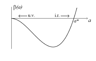
Figure 1: Conventional sketch of “the $\beta$ function” in an asymptotically free theory with an infrared fixed point. The couplant flows to zero in the ultraviolet and to $a^{*}$ in the infrared.

The problem, though, is that there is no such thing as “the $\beta$ function.” It is a myth that there is a unique $\beta$ function characterizing a given theory. In fact, away from the origin, $\beta(a)$ depends strongly on the arbitrary choice of renormalization scheme (RS); that is, it depends on the definition adopted for the renormalized coupling constant (couplant) $a\equiv\alpha_{s}/\pi$. While the first two terms of $\beta(a)$ are unique, all the higher coefficients are RS dependent [1]. Whether or not the $\beta$ function has a fixed point is an entirely RS-dependent question [1, 2, 3].

Renormalization-group invariance [4] means that any physical quantity, ${\cal R}$, is, in principle, independent of the RS choice. However, finite-order perturbative approximants to ${\cal R}$ are RS dependent. The idea of “optimized perturbation theory” (OPT) [5] is to find – for a given ${\cal R}$ at a given energy $Q$ and at a given order of perturbation theory – the “optimal” RS in which the perturbative approximant is locally invariant; i.e., stationary under small changes of RS. At second (next-to-leading) order this optimization is simply a precise formulation of the familiar and powerful idea that the renormalization scale $\mu$ should not be kept fixed but should “run” with the experimental energy scale $Q$. At higher orders, though, the optimization procedure also determines optimal values for the higher-order $\beta$-function coefficients, and these evolve as the energy $Q$ is changed. Thus, the optimized $\beta$ function itself evolves.

Hitherto this last point had seemed – even to this author – a technicality, unlikely to overthrow the basic picture that a finite infrared limit in QCD only occurs if “the $\beta$ function” has a fixed point. Such a fixed-point limit of OPT was analyzed in Ref. [2] and was later found to occur in QCD in the third-order $R_{e^{+}e^{-}}$ case [6, 7]. The recent calculation of the fourth-order correction to $R_{e^{+}e^{-}}$ [8] has allowed us in Ref. [9] to investigate OPT at fourth order. For the phenomenologically relevant case of two massless flavours ($n_{f}=2$) we again found fixed-point behaviour with the couplant freezing to a modest value, with the third-order result $0.3\pm 0.3$ [7] now refined to $0.2\pm 0.1$ [9]. See Fig. 2.

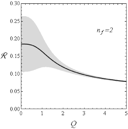
Figure 2: OPT results for ${\cal R}_{e^{+}e^{-}}$(non-singlet) for $n_{f}=2$. The energy $Q$ is in units of $\tilde{\Lambda}_{{\cal R}}$, see Eq. (2.13). The shaded region indicates the error estimate.

Continuing our investigation to higher $n_{f}$ values, however, produced a surprise: a finite infrared limit in OPT can also occur by a quite different mechanism in which the evolution of the $\beta$ function plays an essential role. This “pinch mechanism” produces an extreme “spiking,” rather than a “freezing,” of the couplant as $Q\to 0$; see Fig. 3. The main purpose of this paper is to describe the pinch mechanism and to present numerical results for the infrared limit as a function of $n_{f}$.

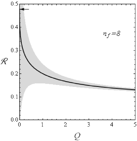
Figure 3: As Fig. 2 but for $n_{f}=8$. The arrow indicates the infrared limit.

In discussing the infrared behaviour of perturbation theory in QCD, one must of course recognize that the results are not directly physical. There exist large nonperturbative, higher-twist terms that perturbation theory is completely blind to. However, it is a longstanding idea [10, 11] that perturbation theory corresponds to some kind of average over hadronic resonances. As shown in Ref. [7], the low-energy $e^{+}e^{-}$ data agrees very nicely, in this sense, with the prediction of OPT that the couplant freezes to a modest value. Moreover, there is a wealth of phenomenological evidence for freezing. We therefore believe that there is some real-world relevance to studying the infrared behaviour of perturbation theory.

It is also interesting theoretically to consider QCD with $n_{f}$ flavours of massless quarks for various $n_{f}$. One reason is to compare with extrapolations from $n_{f}=16{\scriptstyle{\frac{1}{2}}}$ (the Banks-Zaks (BZ) or “small-$b$” expansion [13]), or from $n_{f}=-\infty$ (the “large-$b$” approximation [14, 15]). The other reason is the whole issue of the phase structure of QCD, and other gauge theories, as a function of $n_{f}$ [16] – [20].

We begin by briefly reviewing the key ingredients of OPT [5] in Sect. 2. (See Ref. [9] for a fuller account.) Sections 3 and 4 respectively describe the fixed-point and pinch mechanisms whereby fourth-order OPT produces a finite $Q=0$ limit. Numerical results are presented in Sect. 5. Sect. 6 describes the approach to the $Q=0$ limit and Sect. 7 briefly discusses the possible implications of the results.

2 Optimized perturbation theory

The $\beta$ function, of some general RS, is written as

$$\beta(a)\equiv\mu\frac{da}{d\mu}=-ba^{2}B(a),$$ (2.1)

with

$$B(a)=(1+ca+c_{2}a^{2}+c_{3}a^{3}+\ldots).$$ (2.2)

The first two coefficients of the $\beta$ function are RS invariant [1] and are given by [21, 22]

$$b=\frac{(33-2n_{f})}{6},\quad\quad c=\frac{153-19n_{f}}{2(33-2n_{f})}.$$ (2.3)

The higher $\beta$-function coefficients $c_{2},c_{3},\ldots$ are RS dependent: together with $\tau$,

$$\tau\equiv b\ln(\mu/{\tilde{\Lambda}}),$$ (2.4)

they parametrize the RS choice.

The $\tilde{\Lambda}$ parameter in $\tau$ arises as the constant of integration in the integrated $\beta$-function (int-$\beta$) equation

$$\tau=K(a),$$ (2.5)

where

$$K(a)\equiv\frac{1}{a}+c\ln(\mid\!c\!\mid\!a)-\int_{0}^{a}\frac{dx}{x^{2}}\left(\frac{1}{B(x)}-1+cx\right).$$ (2.6)

This form of $K(a)$, completely equivalent to our previous definition [5, 9], is more convenient when $c$ may be negative. The $\tilde{\Lambda}$ parameter thus defined is RS dependent, but it can be converted between different schemes exactly by the Celmaster-Gonsalves relation [23].

The physical quantity considered here is the $e^{+}e^{-}$ hadronic cross-section ratio $R_{e^{+}e^{-}}(Q)$ at a total c.m. energy $Q$. Neglecting quark masses, this has the form $R_{e^{+}e^{-}}=3\sum q_{i}^{2}(1+{\cal R})$ with

$${\cal R}=a(1+r_{1}a+r_{2}a^{2}+r_{3}a^{3}+\ldots).$$ (2.7)

(Actually, in this paper we will consider only the “non-singlet” part of ${\cal R}$; that is, we drop the terms proportional to $\left(\sum q_{i}\right)^{2}$. This makes very little difference for $0\leq n_{f}\leq 6$ and allows us to discuss higher $n_{f}$’s without needing to specify the electric charges of the fictitious, additional quarks.)

Since it is a physical quantity, ${\cal R}$ satisfies a set of RG equations [5]

$$\frac{\partial{\cal R}}{\partial\tau}=\left(\left.\frac{\partial}{\partial\tau}\right|_{a}+\frac{\beta(a)}{b}\frac{\partial}{\partial a}\right){\cal R}\,=0, \quad\quad``j=1{\mbox{\rm''}},$$

$$\frac{\partial{\cal R}}{\partial c_{j}}=\left(\left.\frac{\partial}{\partial c_{j}}\right|_{a}+\beta_{j}(a)\frac{\partial}{\partial a}\right){\cal R}=0, \quad\quad j=2,3,\ldots.$$

The first of these (“$j=1$”) is the familiar RG equation expressing the invariance of ${\cal R}$ under changes of renormalization scale $\mu$. The other equations express the invariance of ${\cal R}$ under other changes in the choice of RS. The $\beta_{j}(a)$ functions, defined as $\partial a/\partial c_{j}$, are given by

$$\beta_{j}(a)\equiv\frac{a^{j+1}}{(j-1)}B_{j}(a),$$ (2.9)

with

$$B_{j}(a)=\frac{(j-1)}{a^{j-1}}B(a)I_{j}(a),$$ (2.10)

where

$$I_{j}(a)\equiv\int_{0}^{a}dx\,\frac{x^{j-2}}{B(x)^{2}}.$$ (2.11)

The $B_{j}(a)$ functions have expansions that start $1+O(a)$. (Note that for $j\to 1_{+}$ one naturally finds $B_{1}(a)=B(a)$.)

The RG equations (2) imply that certain combinations of ${\cal R}$ and $\beta$-function coefficients are RS invariants. Up to fourth order these are:

$$\tilde{\rho}_{1} = c,\quad\quad{\mbox{\rm and}}\quad\quad\boldsymbol{\rho}_{1}(Q)=\tau-r_{1},$$

$$\tilde{\rho}_{2} = c_{2}+r_{2}-cr_{1}-r_{1}^{2},$$ (2.12)

$$\tilde{\rho}_{3} = c_{3}+2r_{3}-2c_{2}r_{1}-6r_{2}r_{1}+cr_{1}^{2}+4r_{1}^{3}.$$

The numerical values of the $\tilde{\rho}_{2},\tilde{\rho}_{3}$ invariants (see Table 1 below) can be obtained from the $\overline{\rm MS}$ calculations of $c_{2},c_{3}$ [24, 25] and $r_{1},r_{2},r_{3}$ [26, 27, 8], with all dependence on the arbitrary $\overline{\rm MS}$ choice dropping out.

$Q$ dependence enters only through $\boldsymbol{\rho}_{1}(Q)$, which can be conveniently expressed as

$$\boldsymbol{\rho}_{1}(Q)=b\ln(Q/\tilde{\Lambda}_{{\cal R}}),$$ (2.13)

where $\tilde{\Lambda}_{{\cal R}}$ is a characteristic scale specific to the particular physical quantity ${\cal R}$. It can be related back to the traditionally defined $\Lambda_{\scriptscriptstyle{\overline{\rm MS}}}$ parameter by the exact relation

$$\ln(\tilde{\Lambda}_{{\cal R}}/\Lambda_{\scriptscriptstyle{\overline{\rm MS}}})=\frac{r_{1}^{{\scriptscriptstyle{\overline{\rm MS}}}}}{b}-(c/b)\ln(2\!\mid\!c\!\mid\!/b).$$ (2.14)

Note that the infrared limit corresponds to $\boldsymbol{\rho}_{1}(Q)\to-\infty$.

The $(k+1)^{th}$-order approximation, ${\cal R}^{(k+1)}$, in some general RS, is defined by truncating the ${\cal R}$ and $\beta$ series after the $r_{k}$ and $c_{k}$ terms, respectively. Because of these truncations, the resulting approximant depends on RS. “Optimization” [5] corresponds to finding the stationary point where the approximant is locally insensitive to small RS changes, i.e., finding the “optimal” RS in which the RG equations (2) are satisfied by ${\cal R}^{(k+1)}$ with no remainder. The resulting optimization equations [5] were recently solved for the optimized $\bar{r}_{m}$ coefficients [9].

[A note about notation: An overbar can be used to explicitly distinguish optimized from generic quantities, but we shall generally omit these below, leaving it understood that all quantities are the optimized ones at $(k+1)^{th}$ order. The one exception is the symbol “$a$,” which we employ merely as a dummy argument. Thus, we can discuss “the $\beta(a)$ function” in basically the traditional sense as a function of a single variable, $a$, with definite coefficients, $c_{j}=\bar{c}_{j}$; the key difference, though, is that the $\bar{c}_{j}$ coefficients will themselves evolve as the energy $Q$ changes.]

The optimized $r_{m}$ coefficients are given in terms of the optimized couplant $\bar{a}$ and the optimized $c_{j}$ coefficients by [9]:

$$(m+1)r_{m}\bar{a}^{m}=\frac{1}{B_{k}(\bar{a})}\left(H_{k-m}(\bar{a})-H_{k-m+1}(\bar{a})\right),\quad\quad\quad m=0,1,\ldots,k,$$ (2.15)

where

$$H_{i}(a)\equiv\sum_{j=0}^{k-i}c_{j}a^{j}\left(\frac{i-j-1}{i+j-1}\right)B_{i+j}(a),\quad\quad\quad i=(1),2,\ldots,k,$$ (2.16)

with $c_{0}\equiv 1$, $c_{1}\equiv c$. $H_{1}$ is to be understood as the limit $i\to 1$ of the above formula, and $H_{0}\equiv 1$ and $H_{k+1}\equiv 0$. At fourth order ($k=3$) the $H$’s are explicitly given by

$$H_{1}=B-caB_{2}-c_{2}a^{2}B_{3},\quad H_{2}=B_{2},\quad H_{3}=B_{3},$$ (2.17)

and the optimized $r_{m}$ coefficients are given by

$$2r_{1}a=\frac{H_{2}-H_{3}}{H_{3}},\quad 3r_{2}a^{2}=\frac{H_{1}-H_{2}}{H_{3}},\quad 4r_{3}a^{3}=\frac{1-H_{1}}{H_{3}},$$ (2.18)

with $a=\bar{a}$.

The optimized $r_{m}$ and $c_{j}$ coefficients must also be constrained to yield the $\tilde{\rho}_{n}$ invariants of Eq. (2.12). The iterative algorithm outlined in Ref. [9] can be used to solve numerically for the optimized coefficients, and thereby obtain the optimized result, at any given $Q$ value. In the $Q\to 0$ limit these steps can be carried out analytically, as discussed in the next two sections.

3 Fixed-point mechanism

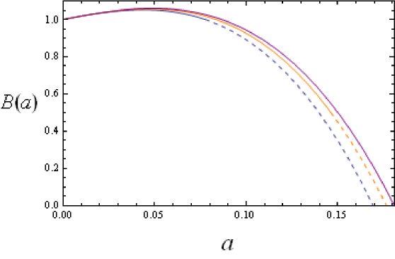
Figure 4: The evolving optimized $B(a)\equiv\beta(a)/(-ba^{2})$ function at fourth order for $n_{f}=2$. The upper, solid curve is the $Q=0$ limiting form with a fixed point at $a^{*}=0.180844$. The two lower curves correspond to larger $Q$ values, and are shown dashed when $a>\bar{a}$.

A finite $Q\to 0$ limit for ${\cal R}(Q)$ can occur by essentially the familiar fixed-point mechanism, with the optimized $B(a)$ function manifesting a simple zero at $a=a^{*}$ (see Fig. 4). The limiting behaviour can be analyzed as follows [2]. For $a$ close to $a^{*}$ one can linearize $B(a)$ as

$$B(a)\approx\sigma(a^{*}-a),$$ (3.1)

where $\sigma$ is some positive constant (directly related to $\gamma^{*}$, the slope of the $\beta$ function at its fixed point; $\gamma^{*}=b{a^{*}}^{2}\sigma$). The integrals $I_{j}(a)$ of Eq. (2.11) will then diverge in the infrared limit, $a\to a^{*}$:

$$I_{j}(a)\to\int_{0}^{a}\!dx\frac{x^{j-2}}{\sigma^{2}(a^{*}-x)^{2}}\to\frac{{a^{*}}^{j-2}}{\sigma^{2}}\frac{1}{(a^{*}-a)}.$$ (3.2)

Substituting in $B_{j}(a)$, Eq. (2.10), one finds that the $\frac{1}{(a^{*}-a)}$ factor is cancelled by the $(a^{*}-a)$ factor in $B(a)$, yielding

$$B_{j}(a)\to\frac{(j-1)}{\sigma a^{*}}.$$ (3.3)

This result corresponds to $\partial a^{*}/\partial c_{j}\to{a^{*}}^{j}/\sigma$, which indeed follows directly [2] by taking $\partial/\partial c_{j}$ (with the other $c_{i}$’s held constant) of the $(k+1)^{th}$-order fixed-point condition

$$B(a^{*})=\sum_{i=0}^{k}c_{i}{a^{*}}^{i}=0.$$ (3.4)

The slope parameter $\sigma$ is given by

$$\sigma=\left.-B^{\prime}(a)\right|_{a=a^{*}}=-\sum_{j=0}^{k}jc_{j}{a^{*}}^{j-1}=\sum_{j=0}^{k-1}(k-j)c_{j}{a^{*}}^{j-1},$$ (3.5)

where the last step uses the fixed-point condition (3.4) to eliminate $c_{k}$. With the limiting $B_{j}$’s from Eq. (3.3) one can construct the $H_{j}$’s and hence the limiting values of the optimized $r_{m}$ coefficients.

At fourth order ($k=3$) one obtains

$$r_{1}^{*}=-\frac{1}{4a^{*}},\quad r_{2}^{*}=-\frac{(1+ca^{*}+2c_{2}^{*}{a^{*}}^{2})}{6{a^{*}}^{2}},\quad r_{3}^{*}=-\frac{3}{8}c_{3}^{*}.$$ (3.6)

By substituting in the definitions of $\tilde{\rho}_{2},\tilde{\rho}_{3}$, Eq. (2.12), one can then find $c_{2}^{*},c_{3}^{*}$ in terms of $a^{*}$ and those invariants. The fixed-point condition above can then be expressed entirely in terms of invariants as [2]

$$\frac{83}{64}+\frac{13}{16}ca^{*}+\frac{3}{4}\tilde{\rho}_{2}{a^{*}}^{2}+2\tilde{\rho}_{3}{a^{*}}^{3}=0.$$ (3.7)

The relevant $a^{*}$ is the smallest positive root of this equation. The final result for the limiting value of ${\cal R}$ at fourth order can then be simplified to [2]

$${{\cal R}^{*}}=a^{*}\left(\frac{249}{256}+\frac{13}{64}ca^{*}+\frac{1}{16}\tilde{\rho}_{2}{a^{*}}^{2}\right).$$ (3.8)

Eq. (3.7) turns out to have no acceptable root when $n_{f}$ is $7,\ldots,15$. (For $n_{f}=15$ there is a positive root but it gives a negative slope $\sigma$, which is unphysical.) Nevertheless, going to ever lower $Q$ values with the optimization procedure, one does find that the optimized result remains bounded as $Q\to 0$. How this happens is the topic of the next section.

4 Pinch mechanism

The essence of the pinch mechanism is illustrated in Fig. 5, which shows the evolution of the optimized $B(a)$ function in the $n_{f}=8$ case. As $Q$ is lowered the optimized $c_{2},c_{3}$ coefficients change so that $B(a)$ develops a minimum — which, in the limit $Q\to 0$, just touches the horizontal axis at a “pinch point,” $a_{\rm p}$. Although this point is then a double root of $B(a)=0$, it does not represent a fixed point. The infrared-limit of the optimized couplant is not $a_{\rm p}$ but a larger value, $a^{\star}$, dubbed the “unfixed point” to stress that it is not a zero of the $\beta$ function.

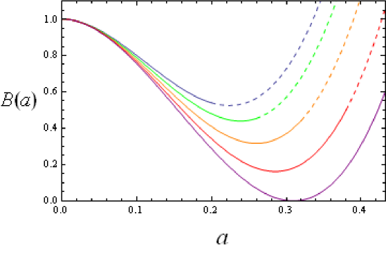
Figure 5: The evolving optimized $B(a)\equiv\beta(a)/(-ba^{2})$ function at fourth order for $n_{f}=8$. The curves, from top to bottom, are for descending $Q$ values. They are shown dashed for $a>\bar{a}$. The lowest curve is the infrared-limiting form, with the pinch point at $a_{\rm p}=0.3094$ and the unfixed point at $a^{\star}=0.432267$.

One can understand this infrared behaviour analytically as follows. $B(a)$ can be approximated around its minimum (at, or nearly at, the pinch point $a_{\rm p}$) by

$$B(a)\approx\eta\left((a-a_{\rm p})^{2}+\delta^{2}\right),$$ (4.1)

where $\delta\to 0$ as $Q\to 0$ and $\eta$ is some positive constant. Thus the integral for the $K(a)$ function in Eq. (2.6) becomes dominated by a “resonant peak”:

$$-\int\frac{dx}{x^{2}}\frac{1}{\eta\left((x-a_{\rm p})^{2}+\delta^{2}\right)}\approx-\frac{1}{a_{\rm p}^{2}\eta}\frac{\pi}{\delta}+\mbox{\rm finite}.$$ (4.2)

Therefore, in the $Q\to 0$ limit (where $\boldsymbol{\rho}_{1}(Q)=K(a)-r_{1}$ tends to $-\infty$), the $\delta$ parameter vanishes $\propto 1/\!\mid\!\ln Q\!\mid$.

The integrals $I_{j}(a)$ of Eq. (2.11) are also dominated by a huge peak in their integrands around $a_{\rm p}$:

$$I_{j}(a)\approx\int\!dx\frac{x^{j-2}}{\left(\eta\left((a-a_{\rm p})^{2}+\delta^{2}\right)\right)^{2}}\approx\frac{a_{\rm p}^{j-2}}{\eta^{2}}\frac{\pi}{2\delta^{3}}.$$ (4.3)

One can thus obtain the $\delta\to 0$ behaviour of the $B_{j}(a)$ and hence the $H_{j}$ functions. (Note that the $B(a)/a^{j-1}$ factor in Eq. (2.10) will involve the limiting value of $a$, which is $a^{\star}$ and not $a_{\rm p}$.) While the $B_{j}$’s and $H_{j}$’s diverge, the $1/\delta^{3}$ factors cancel out, as does $\eta$, in Eq. (2.15), leaving finite limiting values for the optimized $r_{m}$ coefficients.

At fourth order ($k=3$) one finds

$$2r_{1}^{\star} = \frac{(a^{\star}-2a_{\rm p})}{2a^{\star}a_{\rm p}},$$

$$3r_{2}^{\star} = -\frac{1}{2a^{\star}a_{\rm p}}\left(1+ca^{\star}+2c_{2}^{\star}a^{\star}a_{\rm p}\right),$$ (4.4)

$$4r_{3}^{\star} = \frac{(c+2c_{2}^{\star}a_{\rm p})}{2a^{\star}a_{\rm p}}.$$

The infrared limit of the fourth-order $B(a)$ function is

$$B^{\star}(a)=1+ca+c_{2}^{\star}a^{2}+c_{3}^{\star}a^{3}.$$ (4.5)

The pinch point $a_{\rm p}$ is where this function touches the $a$ axis (see Fig. 5) and hence satisfies the two equations $B^{\star}(a)=0$ and $dB^{\star}/da=0$ at $a=a_{\rm p}$. These two equations yield

$$c_{2}^{\star} = -\frac{(3+2ca_{\rm p})}{a_{\rm p}^{2}},$$

$$c_{3}^{\star} = \frac{(2+ca_{\rm p})}{a_{\rm p}^{3}}.$$

Substituting Eqs. (4.4) and (LABEL:clim) into the definitions of the $\tilde{\rho}_{2}$ and $\tilde{\rho}_{3}$ in Eq. (2.12) yields two equations:

$$12a_{\rm p}^{2}-4(1+6ca_{\rm p})a^{\star}a_{\rm p}+(99+84ca_{\rm p}+48\tilde{\rho}_{2}a_{\rm p}^{2}){a^{\star}}^{2}=0,$$ (4.7)

$$8a_{\rm p}^{3}-4(1+ca_{\rm p})a^{\star}a_{\rm p}^{2}+2(13+12ca_{\rm p}){a^{\star}}^{2}a_{\rm p}+(-33-21ca_{\rm p}+16\tilde{\rho}_{3}a_{\rm p}^{3}){a^{\star}}^{3}=0.$$ (4.8)

These two equations determine $a_{\rm p}$ and $a^{\star}$ in terms of the invariants $c,\tilde{\rho}_{2},\tilde{\rho}_{3}$. One can manipulate these equations to find $a_{\rm p}$ in terms of $a^{\star}$ as

$$a_{\rm p}=\frac{a^{\star}(62+14ca^{\star}+(21c^{2}-148\tilde{\rho}_{2}){a^{\star}}^{2}-6(7\tilde{\rho}_{2}c-33\tilde{\rho}_{3}){a^{\star}}^{3})}{2(2-31ca^{\star}+3(4\tilde{\rho}_{2}-c^{2}){a^{\star}}^{2}+4(6\tilde{\rho}_{2}c+\tilde{\rho}_{3}){a^{\star}}^{3}+12(4\tilde{\rho}_{2}^{2}-7\tilde{\rho}_{3}c){a^{\star}}^{4})},$$ (4.9)

with $a^{\star}$ given by a 6th-order polynomial equation:

$$0 = 11680+2224ca^{\star}+3(5997c^{2}-17264\tilde{\rho}_{2}){a^{\star}}^{2}+$$

$${}+2(8235c^{3}-33624\tilde{\rho}_{2}c+36976\tilde{\rho}_{3}){a^{\star}}^{3}+$$

$${}+18(147c^{4}-2184\tilde{\rho}_{2}c^{2}+4640\tilde{\rho}_{2}^{2}+502\tilde{\rho}_{3}c){a^{\star}}^{4}+$$

$${}+324(-49\tilde{\rho}_{2}c^{3}+152\tilde{\rho}_{2}^{2}c+161\tilde{\rho}_{3}c^{2}-528\tilde{\rho}_{3}\tilde{\rho}_{2}){a^{\star}}^{5}+$$

$${}+108(-147\tilde{\rho}_{2}^{2}c^{2}+528\tilde{\rho}_{2}^{3}+343\tilde{\rho}_{3}c^{3}-1386\tilde{\rho}_{3}\tilde{\rho}_{2}c+1089\tilde{\rho}_{3}^{2}){a^{\star}}^{6}.$$

The final result for the infrared limit of ${\cal R}$ at fourth order can be expressed as

$${\cal R}^{\star}=\frac{a^{\star}(2a^{\star}a_{\rm p}+12{a_{\rm p}}^{2}+3{a^{\star}}^{2}(2+ca_{\rm p}))}{24{a_{\rm p}}^{2}}.$$ (4.11)

Note that $a^{\star}\geq a_{\rm p}$ is needed for this solution to be relevant. One can check that the special case $a^{\star}=a_{\rm p}$ is indeed the boundary between the pinch mechanism and the fixed-point mechanism, and corresponds to where $\gamma^{*}=0$. From such an analysis one can determine the precise $n_{f}$ values where the switchover from one mechanism to the other takes place.

It is possible, in principle, for the pinch mechanism to occur at third order; see Appendix A.

5 Numerical results

The inputs to our numerical calculations are collected in Table 1, which lists the RS-invariant quantities $c$, $\tilde{\rho}_{2}$, $\tilde{\rho}_{3}$ for integer $n_{f}$ from $0$ to $16$. These values are obtained from the Feynman-diagram calculations of Ref. [8] and earlier authors [22], [24]–[27]. (The singlet terms, proportional to $(\sum q_{i})^{2}$ have been dropped.)

Table 2 gives our results for the infrared limit of ${\cal R}$ for $n_{f}=0,\ldots,16$. The quoted error estimate on ${\cal R}$ corresponds to the last term, $r_{3}a^{4}$, of the truncated perturbation series, evaluated in the optimized RS [7, 9]. Also listed are values of the fixed-point, or the unfixed-point and pinch-point. (The critical exponent $\gamma^{*}$ will be discussed later.) The fixed-point mechanism operates for $n_{f}<6.727$, then the pinch mechanism takes over until $n_{f}=15.191$, when the fixed-point mechanism returns and operates until $n_{f}=16{\scriptstyle{\frac{1}{2}}}$ when $a^{*}\to 0$.

Table 3 gives the optimized coefficients, weighted by the appropriate power of $\bar{a}$, in both the $\beta$-function and ${\cal R}$ series. This information is important for anyone wishing to check our results and also displays the behaviour of the truncated series for both ${\cal R}$ and $B(a)$. This behaviour is, at best, only marginally satisfactory: Clearly, by going to the $Q\to 0$ limit we are pushing low-order perturbation theory well beyond its comfort zone. Nevertheless, all things considered, we believe that the results are credible within the large uncertainties quoted in Table 2 and illustrated in Figs. 2 and 3. In particular, we believe that the dramatic $Q\to 0$ spike produced by the pinch mechanism is real; the very large error estimate just cautions that the height of the spike is very uncertain; it might be somewhat smaller, or it might well be considerably bigger.

$n_{f}$	$c$	$\tilde{\rho}_{2}$	$\tilde{\rho}_{3}$
$0$	$2\cdot 31818$	$-7\cdot 066723$	$-184\cdot 37823$
$1$	$2\cdot 16129$	$-8\cdot 397865$	$-147\cdot 27522$
$2$	$1\cdot 98276$	$-9\cdot 842342$	$-113\cdot 85683$
$3$	$1\cdot 77778$	$-11\cdot 417129$	$-83\cdot 83139$
$4$	$1\cdot 54$	$-13\cdot 144635$	$-56\cdot 87785$
$5$	$1\cdot 26087$	$-15\cdot 055062$	$-32\cdot 63303$
$6$	$0\cdot 928571$	$-17\cdot 190118$	$-10\cdot 67155$
$7$	$0\cdot 526316$	$-19\cdot 609073$	$9\cdot 52688$
$8$	$0\cdot 029412$	$-22\cdot 399086$	$28\cdot 63336$
$9$	$-0\cdot 6$	$-25\cdot 693806$	$47\cdot 57023$
$10$	$-1\cdot 42308$	$-29\cdot 709122$	$67\cdot 70445$
$11$	$-2\cdot 54545$	$-34\cdot 817937$	$91\cdot 25169$
$12$	$-4\cdot 16667$	$-41\cdot 724622$	$122\cdot 21944$
$13$	$-6\cdot 71429$	$-51\cdot 938541$	$168\cdot 96670$
$14$	$-11\cdot 3$	$-69\cdot 384046$	$252\cdot 90695$
$15$	$-22\cdot 0$	$-108\cdot 450422$	$452\cdot 02327$
$16$	$-75\cdot 5$	$-298\cdot 641242$	$1466\cdot 56390$

Table 1: Values of the invariants for ${\cal R}_{e^{+}e^{-}}$(non-singlet) obtained from the calculations of Ref. [8], [22], [24]–[27].

$n_{f}$	$a^{*}$	$a^{\star}$	$a_{\rm p}$	${\cal R}^{*}$	$\gamma^{*}$
$0$	$0.158279$	${\scriptstyle(0.1334)}$	${\scriptstyle(2.50)}$	$0.164\pm 0.083$	$3.28$
$1$	$0.168688$	${\scriptstyle(0.1465)}$	${\scriptstyle(1.20)}$	$0.174\pm 0.083$	$3.20$
$2$	$0.180844$	${\scriptstyle(0.1633)}$	${\scriptstyle(0.832)}$	$0.185\pm 0.080$	$3.09$
$3$	$0.195462$	${\scriptstyle(0.1857)}$	${\scriptstyle(0.651)}$	$0.199\pm 0.073$	$2.94$
$4$	$0.213910$	${\scriptstyle(0.2162)}$	${\scriptstyle(0.540)}$	$0.214\pm 0.059$	$2.73$
$5$	$0.239369$	${\scriptstyle(0.2588)}$	${\scriptstyle(0.462)}$	$0.235\pm 0.028$	$2.40$
$6$	$0.282493$	${\scriptstyle(0.3164)}$	${\scriptstyle(0.402)}$	$0.266\pm 0.051$	$1.76$
$7$	—	$0.383293$	$0.3525$	$0.35\pm 0.37$	$0$
$8$	—	$0.432267$	$0.3094$	$0.48\pm 0.64$	$0$
$9$	—	$0.429519$	$0.2702$	$0.52\pm 0.75$	$0$
$10$	—	$0.376034$	$0.2341$	$0.44\pm 0.61$	$0$
$11$	—	$0.301883$	$0.2001$	$0.32\pm 0.38$	$0$
$12$	—	$0.229746$	$0.1673$	$0.21\pm 0.21$	$0$
$13$	—	$0.166832$	$0.1346$	$0.14\pm 0.11$	$0$
$14$	—	$0.112784$	$0.1007$	$0.08\pm 0.05$	$0$
$15$	${\scriptstyle(0.0674)}$	$0.065248$	$0.0642$	$0.043\pm 0.015$	$0$
$16$	$0.020058$	${\scriptstyle(0.0215)}$	${\scriptstyle(0.0228)}$	$0.013\pm 0.001$	$0.001$

Table 2: Infrared-limit results for ${\cal R}_{e^{+}e^{-}}$(non-singlet) in OPT at fourth order for different $n_{f}$ values. For $n_{f}=0,\ldots,6$ and $n_{f}=16$ the limit is governed by a fixed point at $a^{*}$: For $n_{f}=7,\ldots,15$ it arises from the pinch mechanism, with an “unfixed point” at $a^{\star}$ and a “pinch point” at $a_{\rm p}$. (The $a^{\star}$ equation has solutions outside this range, giving the values in parentheses, but these violate the $a^{\star}>a_{\rm p}$ requirement. Also, the fixed-point equation has a solution for $n_{f}=15$, but one that violates the $\gamma^{*}\geq 0$ requirement.) The last column gives values for the critical exponents $\gamma^{*}$ which characterize the power-law approach of ${\cal R}$ to its fixed-point limit; ${\cal R}^{*}-{\cal R}\propto Q^{\gamma^{*}}$. In the unfixed-point case one finds instead ${\cal R}^{\star}-{\cal R}\propto 1/\mid\!\ln Q\!\mid^{2}$.

$n_{f}$	$ca$	$c_{2}a^{2}$	$c_{3}a^{3}$	$r_{1}a$	$r_{2}a^{2}$	$r_{3}a^{3}$
$0$	$0\cdot 36692$	$0\cdot 032328$	$-1\cdot 39925$	$-0\cdot 25$	$-0\cdot 238596$	$0\cdot 524718$
$1$	$0\cdot 364583$	$-0\cdot 060272$	$-1\cdot 30431$	$-0\cdot 25$	$-0\cdot 20734$	$0\cdot 489117$
$2$	$0\cdot 35857$	$-0\cdot 183906$	$-1\cdot 17466$	$-0\cdot 25$	$-0\cdot 165126$	$0\cdot 440499$
$3$	$0\cdot 347489$	$-0\cdot 353982$	$-0\cdot 993507$	$-0\cdot 25$	$-0\cdot 106587$	$0\cdot 372565$
$4$	$0\cdot 329421$	$-0\cdot 599622$	$-0\cdot 729799$	$-0\cdot 25$	$-0\cdot 021696$	$0\cdot 273674$
$5$	$0\cdot 301813$	$-0\cdot 987899$	$-0\cdot 313913$	$-0\cdot 25$	$0\cdot 112331$	$0\cdot 117717$
$6$	$0\cdot 262315$	$-1\cdot 74675$	$0\cdot 484438$	$-0\cdot 25$	$0\cdot 371865$	$-0\cdot 181664$
$7$	$0\cdot 201733$	$-3\cdot 98554$	$2\cdot 80955$	$-0\cdot 228168$	$1\cdot 11073$	$-0\cdot 968966$
$8$	$0\cdot 012714$	$-5\cdot 89311$	$5\cdot 48146$	$-0\cdot 150668$	$1\cdot 72852$	$-1\cdot 47106$
$9$	$-0\cdot 257711$	$-6\cdot 75979$	$7\cdot 37992$	$-0\cdot 102638$	$2\cdot 05663$	$-1\cdot 74115$
$10$	$-0\cdot 535126$	$-6\cdot 02116$	$6\cdot 90794$	$-0\cdot 098434$	$1\cdot 8826$	$-1\cdot 61273$
$11$	$-0\cdot 768429$	$-4\cdot 50798$	$5\cdot 11621$	$-0\cdot 122888$	$1\cdot 44444$	$-1\cdot 27189$
$12$	$-0\cdot 957273$	$-3\cdot 02694$	$3\cdot 3723$	$-0\cdot 156741$	$0\cdot 999204$	$-0\cdot 921032$
$13$	$-1\cdot 12016$	$-1\cdot 83192$	$2\cdot 08731$	$-0\cdot 190139$	$0\cdot 635461$	$-0\cdot 631526$
$14$	$-1\cdot 27446$	$-0\cdot 907359$	$1\cdot 20999$	$-0\cdot 220064$	$0\cdot 353673$	$-0\cdot 405223$
$15$	$-1\cdot 43545$	$-0\cdot 183663$	$0\cdot 619584$	$-0\cdot 245711$	$0\cdot 135041$	$-0\cdot 228425$
$16$	$-1\cdot 51438$	$0\cdot 352822$	$0\cdot 161556$	$-0\cdot 25$	$-0\cdot 031878$	$-0\cdot 060584$

Table 3: Terms in the optimized $\beta$-function and ${\cal R}$ series in the infrared limit ($a=a^{*}$ or $a^{\star}$, as appropriate).

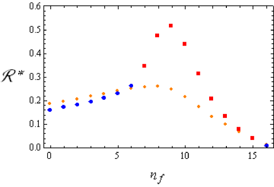
Figure 6: Infrared limiting values of ${\cal R}_{e^{+}e^{-}}$(non-singlet) in fourth-order OPT, as a function of $n_{f}$. The large dark circles and squares are, respectively, from fixed-point and pinch mechanisms. (The smaller points are the corresponding results in the FAC scheme.) Estimated uncertainties are large — about 50% at low $n_{f}$, rising to 150% around $n_{f}=9$, then shrinking to about 10% at $n_{f}=16$.

Fig. 6 plots the infrared limiting ${\cal R}$ values against $n_{f}$. The large “bump” around $n_{f}\approx 9$ is where the pinch mechanism produces really dramatic spiking of ${\cal R}$ as $Q\to 0$, as seen in Fig. 3 for $n_{f}=8$. If, instead of ${\cal R}^{*}$, we had plotted ${\cal R}(Q)$ for some low, but finite $Q$ — say around ${\scriptstyle{\frac{1}{2}}}\tilde{\Lambda}_{\cal R}$ — the bump would not have appeared and the points would have been close to the smaller, fainter points.

Those smaller points are the infrared-limiting results in the FAC (fastest apparent convergence) or “effective charge” [28] scheme. That scheme is defined such that all the $r_{m}$ coefficients vanish, giving ${\cal R}=a_{{\rm FAC}}(1+0+0+\ldots)$. The FAC $\beta$ function’s coefficients then coincide with the $\tilde{\rho}_{n}$ invariants (and so can be read off from Table 1). Since those coefficients do not evolve with $Q$, the infrared limit in FAC is simply obtained by finding the fixed point of the FAC $\beta$ function. Many authors (e.g. [29]) have observed that, at low orders, FAC seems to yield very similar results to OPT. That observation holds true here, certainly at low $n_{f}$ and close to $n_{f}=16{\scriptstyle{\frac{1}{2}}}$. It also holds in the range $7\lesssim n_{f}\lesssim 13$ at energies $Q\gtrsim{\scriptstyle{\frac{1}{2}}}\tilde{\Lambda}_{\cal R}$, as noted above. However, the FAC scheme does not see the extreme spiking at $Q=0$. While it is still true, because the error estimates (see Table 2) are so large in this region, that OPT and FAC infrared results agree within the error estimate, it is fair to say that the presence or absence of the spike is a qualitative difference in the predictions of the two schemes. (We expect other distinct differences between OPT and FAC to emerge at higher orders since the FAC $\beta$ function is almost certainly factorially divergent, whereas an “induced convergence” mechanism is conjectured to operate in OPT [30].)

6 Approach to the $Q=0$ limit

Proper analysis of the subleading terms governing the approach to the $Q=0$ limit, in both the fixed- and unfixed-point cases, is surprisingly subtle and intricate. We postpone details to a future publication and report here only the main results.

The usual lore is that the approach to a fixed point is described by a power law with a critical exponent given by the slope of the $\beta$ function at the fixed point:

$${\cal R}^{*}-{\cal R}\propto Q^{\gamma^{*}}\quad{\mbox{{\rm with}}}\quad\gamma^{*}=\beta^{\prime}(a^{*})\equiv\left.\frac{d\beta(a)}{da}\right|_{a=a^{*}}.$$ (6.1)

The derivation of this result, in a fixed RS, and the proof that $\beta^{\prime}(a^{*})$ is invariant under RS changes [31] is subject to some caveats — which, as Chýla [3] has rightly pointed out, are not necessarily to be viewed as very rare exceptions. In OPT it is far from obvious that the above result will hold because the optimized couplant and optimized $r_{m}$ and $c_{j}$ coefficients have $\epsilon\ln\epsilon$ corrections as they approach their fixed-point limits, where $\epsilon\equiv B(a)$. Remarkably, though, the $\epsilon\ln\epsilon$ terms cancel in ${\cal R}$, leaving

$${\cal R}^{*}-{\cal R}=\frac{a^{*}}{k-1}\epsilon+O(\epsilon^{2}\ln\epsilon)$$ (6.2)

in $(k+1)^{th}$ order. From the int-$\beta$ equation, (2.5), together with the $\boldsymbol{\rho}_{1}(Q)$ definition in Eqs. (2.12), (2.13), one sees that

$$\ln\epsilon=\gamma^{*}\ln Q+{\mbox{\rm const.}},$$ (6.3)

so that $\epsilon$, and hence ${\cal R}^{*}-{\cal R}$, is proportional to $Q^{\gamma^{*}}$ where $\gamma^{*}$ is the slope of the optimized $\beta$ function at its fixed point: that is, $\gamma^{*}=b{a^{*}}^{2}\sigma$ with $\sigma$ given by Eq. (3.5), evaluated in the optimized scheme. At fourth order this corresponds to

$$\gamma^{*}=ba^{*}(3+2ca^{*}+{c_{2}}^{*}{a^{*}}^{2}).$$ (6.4)

The numerical $\gamma^{*}$ values are reported in Table 2. Note that $\gamma^{*}$ is around $2$ or $3$ for $0\leq n_{f}\leq 6$, so the resulting low-$Q$ behaviour (Fig. 2) is appropriately described as “freezing” of the couplant. However, when $\gamma^{*}$ is very small, as in the $n_{f}=16$ case, one sees instead “spiking” at $Q\to 0$, though not quite as extreme as the logarithmic spiking produced by the pinch mechanism.

In the unfixed-point case we find, after a lengthy calculation, the simple result:

$${\cal R}^{\star}-{\cal R}=\frac{{a^{\star}}^{4}(3+ca_{\rm p})}{2{a_{\rm p}}^{5}}\delta^{2}+O(\delta^{3}).$$ (6.5)

From the int-$\beta$ equation and $\boldsymbol{\rho}_{1}(Q)$ definition we obtain (as in Eq. (4.2))

$$\delta=\frac{\pi}{b}\frac{1}{(3+ca_{\rm p})}\frac{1}{\mid\!\ln Q/\tilde{\Lambda}_{{\cal R}}|}\quad\quad\,{\mbox{\rm as}}\,\,Q\to 0.$$ (6.6)

Therefore

$${\cal R}^{\star}-{\cal R}=\frac{1}{b_{\rm ir}^{2}}\frac{1}{\mid\!\ln Q/\tilde{\Lambda}_{{\cal R}}|^{2}}+O\left(\frac{1}{\mid\!\ln Q\!\mid^{3}}\right),$$ (6.7)

where

$$b_{\rm ir}\equiv\sqrt{2a_{\rm p}(3+ca_{\rm p})}\left(\frac{a_{\rm p}}{a^{\star}}\right)^{2}\frac{b}{\pi}.$$ (6.8)

One way to look at the result is to note that

$$Q\frac{d{\cal R}}{dQ}\sim-2b_{\rm ir}({\cal R}^{\star}-{\cal R})^{3/2}$$ (6.9)

for ${\cal R}$ close to ${\cal R}^{\star}$. Thus, the “physically defined $\beta$ function” associated with ${\cal R}$ is predicted by OPT to have neither a simple nor a double zero, but something in between. An even more intriguing interpretation is to see the low-energy prediction as

$${\cal R}={\cal R}^{\star}-\lambda^{2}\left(1+O(\lambda)\right)$$ (6.10)

with $\lambda\sim 1/(b_{\rm ir}\ln Q)$ viewed as the running coupling constant of some infrared effective theory whose $\beta$ function starts $b_{\rm ir}\lambda^{2}(1+\ldots)$.

7 Discussion

We now briefly discuss the implications of our results. The abrupt change between $n_{f}=6$ and $n_{f}=7$ seems indicative of a phase transition. For $n_{f}\leq 6$ the phase is presumably the one we are familiar with in the real world; colour is confined and chiral symmetry is broken, with the associated goldstone bosons (pions) being massless. Vector mesons ($\rho$’s, etc.) have masses of order $\tilde{\Lambda}$ and their resonant contribution dominates $e^{+}e^{-}\to$ hadrons at low energies. Although the actual $R_{e^{+}e^{-}}\propto 1+{\cal R}$ is very different from the smooth perturbative prediction (Fig. 2), the two agree well after Poggio-Quinn-Weinberg (PQW) smearing [11] is applied to both [7].

For $n_{f}>7$ the effective low-energy theory seems to be a renormalizable theory with a mass scale appearing only in logarithms. The extreme spiking of ${\cal R}$ as $Q\to 0$ (Fig. 3), if viewed as a resonant peak in the vector channel, hints that massless vector bosons are now present. These might be the gluons of an unconfined phase, or they might be massless, colourless vector mesons of a confined phase, perhaps with unbroken chiral symmetry.

Between 15 and 16 flavours our OPT results switch back from unfixed- to fixed-point behaviour. However, it is much less clear that this indicates a phase transition. There is hardly any qualitative difference between the extreme (logarithmic) spiking of the unfixed-point case and the very strong (fractional power-law) behaviour of a fixed-point with a very small $\gamma^{*}$. Note that the theory with $16$ flavours (or $16.4999$, for that matter) is not exactly scale and conformal invariant. While there is a huge range of $Q$ over which the couplant is nearly constant (at a value about $0.78$ of its infrared limit [32]), it does fall to zero (very slowly) as $Q\to\infty$ and it does rise (very abruptly) as $Q\to 0$.

It is beyond the scope of this paper to attempt a detailed comparison with the literature, but we do see some points of resemblance with other approaches [16, 17, 18] and with some firmly established results in supersymmetric QCD [19, 17]. There is also a large literature on lattice Monte-Carlo studies of QCD at large $n_{f}$ values (for recent work, see [20]).

A quick look back at third-order OPT results is in order. There the results for ${\cal R}^{*}$ decreased roughly linearly from $0.4$ to $0$ as $n_{f}$ increased from $0$ to $16{\scriptstyle{\frac{1}{2}}}$ (see Fig. 1 of Ref. [32]). Since the uncertainties were large ($\sim 100\%$ at low $n_{f}$), sizeable changes at fourth order were not unexpected. Nevertheless, it is an interesting surprise to find qualitatively different features — particularly the spiking phenomenon produced by the pinch mechanism, responsible for the prominent bump around $n_{f}\approx 9$ in Fig. 6. Previously, the good agreement of the third-order results with the leading $16{\scriptstyle{\frac{1}{2}}}-n_{f}$ (BZ) expansion led us to suggest [32] that that expansion might remain good down to very low $n_{f}$. That suggestion no longer seems tenable. We would now expect the BZ expansion to break down around $n_{f}\sim 9$, if not sooner.

The fact that the fourth-order results show a rise of ${\cal R}^{*}$ with $n_{f}$ at low $n_{f}$ is interesting. At third order the OPT fixed-point equations would give ${\cal R}^{*}\sim 2.19/b$ in the $n_{f}\to-\infty$ ($b\to\infty$) limit, but that limiting form only applies for $n_{f}\lesssim-200$. At fourth order, the large-$b$ limit of Eqs. (3.7), (3.8) gives ${\cal R}^{*}\sim 0.84/b$, a formula that roughly describes the OPT results up to $n_{f}\approx 6$. (Unfortunately, the large-$b$ resummation method is fraught with subtleties in the infrared region and it remains unclear what it predicts for ${\cal R}^{*}$ [15].)

In closing we would like to stress that the results in this paper are directly the result of applying the method of Ref. [5] to the Feynman-diagram results for $R_{e^{+}e^{-}}$. We have invented nothing new, nor tweaked the method in any way. The freezing or spiking, depending on $n_{f}$, is just what happens when one solves the optimization equations [5] at ever lower $Q$ values. Achieving a finite infrared limit was no part of the motivation for OPT (and was never considered in Ref. [5]), so the fact that it happens is a genuine prediction — and a non-trivial one, as history shows. The “pinch mechanism” (Fig. 5) is another remarkable consequence of OPT. It has serious implications beyond perturbation theory, because it suggests that the phase structure of QCD may not be understandable in the traditional language of fixed points of “the $\beta$ function.”

Appendix A: Pinch mechanism at third order

The pinch mechanism can actually occur even at third order, under certain restrictive conditions. (These conditions are never satisfied in the $e^{+}e^{-}$ QCD case, but for other physical quantities, or other gauge theories, the possibility could arise.) At third order the $B(a)\equiv 1+ca+c_{2}a^{2}$ function can obviously be re-written in the form

$$B(a)=\eta\left((a-a_{\rm p})^{2}+\delta^{2}\right),$$ (A.1)

with

$$\eta=c_{2},\quad\quad\quad-2a_{\rm p}\eta=c,\quad\quad\quad\eta(a_{\rm p}^{2}+\delta^{2})=1.$$ (A.2)

If $\eta=c_{2}$ is positive and $c$ is negative, $B(a)$ has a minimum at a positive $a_{\rm p}=-c/(2c_{2})$ that can become a pinch point if the evolution of the optimized $c_{2}$ coefficient results in $\delta$ tending to zero as $Q\to 0$. The discussion around Eqs. (4.1) – (4.3) then applies, predicting the $\delta\to 0$ forms of the $I_{j}(a)$ integrals, and hence of the $B_{j}(a)$ functions. At this order ($k=2$) Eq. (2.16) yields

$$H_{1}=B-caB_{2},\quad\,H_{2}=B_{2},$$ (A.3)

so that, substituting in Eq. (2.15), one finds

$$2r_{1}^{\star}=-\frac{1+ca^{\star}}{a^{\star}},\quad\,3r_{2}^{\star}=\frac{c}{a^{\star}}.$$ (A.4)

From Eq. (A.2) with $\delta\to 0$ one obtains

$$a_{\rm p}=-\frac{2}{c},\quad\,c_{2}^{\star}=\frac{c^{2}}{4}.$$ (A.5)

Substituting in the definition of $\tilde{\rho}_{2}$ yields a quadratic equation for $a^{\star}$:

$$1-\frac{4}{3}ca^{\star}+4\left(\tilde{\rho}_{2}-\frac{c^{2}}{2}\right){a^{\star}}^{2}=0.$$ (A.6)

The infrared limit of ${\cal R}$ can be written, using Eq. (A.4), as

$${\cal R}^{\star}=\frac{1}{6}a^{\star}(3-ca^{\star}).$$ (A.7)

As noted above, the pinch mechanism requires $c$ to be negative, so Eq. (A.6) will only have a positive root if $\tilde{\rho}_{2}-\frac{c^{2}}{2}$ is negative. Finally, the pinch mechanism requires $a^{\star}>a_{\rm p}$ which requires $\tilde{\rho}_{2}/c^{2}>13/48$ (and for smaller $\tilde{\rho}_{2}$’s the fixed-point mechanism takes over). In summary, the pinch mechanism can operate at third order if and only if

$$c<0\quad\,{\mbox{\rm and}}\quad\,\frac{13}{48}<\frac{\tilde{\rho}_{2}}{c^{2}}<\frac{1}{2}.$$ (A.8)

References

- [1] G. ’t Hooft, in Deeper Pathways in High-Energy Physics, proceedings of Orbis Scientiae 1977, Coral Gables, edited by A. Perlmutter and L. F. Scott (Plenum, New York, 1977).
- [2] J. Kubo, S. Sakakibara, and P. M. Stevenson, Phys. Rev. D 29, 1682 (1984).
- [3] J. Chýla, Phys. Rev. D 38, 3845 (1988).
- [4] E. C. G. Stueckelberg and A. Peterman, Helv. Phys. Acta 26, 449 (1953); M. Gell Mann and F. Low, Phys. Rev. 95, 1300 (1954).
- [5] P. M. Stevenson, Phys. Rev. D 23, 2916 (1981).
- [6] J. Chýla, A. Kataev, and S. A. Larin, Phys. Lett. B 267, 269 (1991).
- [7] A. C. Mattingly and P. M. Stevenson, Phys. Rev. Lett. 69, 1320 (1992); Phys. Rev. D 49, 437 (1994).
- [8] P. A. Baikov, K. G. Chetyrkin, J. H. Kühn, and J. Rittinger, Phys. Lett. B 714, 62 (2012); P. A. Baikov, K. G. Chetyrkin, and J. H. Kühn, Phys. Rev. Lett. 101, 012002 (2008).
- [9] P. M. Stevenson, Nucl. Phys. B 868, 38 (2013).
- [10] E. D. Bloom and F. J. Gilman, Phys. Rev. D 4, 2901 (1971).
- [11] E. C. Poggio, H. R. Quinn, and S. Weinberg, Phys. Rev. D 13, 1958 (1976).
- [12] R. J. Crewther and L. C. Tunstall, arXiv:1203.1321 [hep-ph].
- [13] T. Banks and A. Zaks, Nucl. Phys. B 196, 189 (1982).
- [14] A. Palanques-Mestre and P. Pascual, Commun. Math. Phys. 95, 277 (1984); M. Beneke, Nucl. Phys. B 405, 424 (1993); D. J. Broadhurst, Z. Phys. C 58, 339 (1993).
- [15] C. N. Lovett-Turner and C. J. Maxwell, Nucl. Phys. B 432, 147 (1994); ibid B 452, 188 (1995); P. M. Brooks and C. J. Maxwell, Phys. Rev. D 74, 065012 (2006).
- [16] T. Appelquist, J. Terning, and L. C. R. Wijewardhana, Phys. Rev. Lett. 77, 1214 (1996).
- [17] E. Shuryak, Summary talk at RHIC Summer Studies, Brookhaven, July 1996; arXiv: hep-ph/9609249.
- [18] V. A. Miransky and K. Yamawaki, Phys. Rev. D 55, 5051 (1997) [Erratum-ibid. D 56 3768 (1997)].
- [19] N. Seiberg, Phys. Rev. D 49, 6857 (1994).
- [20] K. Yamawaki, hep-ph 1305.6352; Y. Aoki et al. (LatKMI collab.) hep-lat/1305.6006; Xiao-Yong Jin and R. D. Mawhinney, hep-lat/1304.0312; A. Deuzeman, M. P. Lombardo, K. Miura, T. N. da Silva, and E. Pallante, hep-lat/1304.3245.
- [21] H. D. Politzer, Phys. Rev. Lett. 30, 1346 (1973); D. J. Gross and F. Wilczek, ibid. 30, 1343 (1973); G. ’t Hooft, report at the Marseille Conference Yang-Mills Fields, 1972.
- [22] W. Caswell, Phys. Rev. Lett. 33, 244 (1974); D. R. T. Jones, Nucl. Phys. B 75, 531 (1974); E. S. Egorian and O. V. Tarasov, Theor. Mat. Fiz. 41, 26 (1979).
- [23] W. Celmaster and R. J. Gonsalves, Phys. Rev. D 20, 1420 (1979).
- [24] O. V. Tarasov, A. A. Vladimirov, and A. Yu. Zharkov, Phys. Lett. B 93, 429 (1980); S. A. Larin and J. A. M. Vermaseren, Phys. Lett. B 303, 334 (1993).
- [25] T. van Ritbergen, J. A. M. Vermaseren, and S. A. Larin, Phys. Lett. B 400, 379 (1997).
- [26] K. G. Chetyrkin, A. L. Kataev, and F. V. Tkachov, Phys. Lett. B 85, 277 (1979); M. Dine and J. Sapirstein, Phys. Rev. Lett. 43, 668 (1979); W. Celmaster and R. J. Gonsalves, Phys. Rev. D 21, 3112 (1980).
- [27] L. R. Surguladze and M. A. Samuel, Phys. Rev. Lett. 66, 560 (1991); S. G. Gorishny, A. L. Kataev, and S. A. Larin, Phys. Lett. B 259, 144 (1991).
- [28] G. Grunberg, Phys. Rev. D 29, 2315 (1984); A. Dhar and V. Gupta, Phys. Rev. D 29, 2822 (1984); C. J. Maxwell, arXiv:hep-ph/9908463.
- [29] J. Kubo and S. Sakakibara, Phys. Rev. D 26, 3656 (1982).
- [30] P. M. Stevenson, Nucl. Phys. B 231, 65 (1984); K. Van Acoleyen and H. Verschelde, Phys. Rev. D 69 125006 (2004).
- [31] D. J. Gross, in Methods in Field Theory, edited by R. Balian and J. Zinn-Justin (North-Holland, Amsterdam, 1976).
- [32] P. M. Stevenson, Phys. Lett. B 331, 187 (1994); S. Caveny and P. M. Stevenson, arXiv: hep-ph/9705319.