Inverse Compton X-ray signature of AGN feedback

Abstract

Bright AGN frequently show ultra-fast outflows (UFOs) with outflow velocities $v_{\rm out}\sim 0.1c$. These outflows may be the source of AGN feedback on their host galaxies sought by galaxy formation modellers. The exact effect of the outflows on the ambient galaxy gas strongly depends on whether the shocked UFOs cool rapidly or not. This in turn depends on whether the shocked electrons share the same temperature as ions (one temperature regime; 1T) or decouple (2T), as has been recently suggested. Here we calculate the Inverse Compton spectrum emitted by such shocks, finding a broad feature potentially detectable either in mid-to-high energy X-rays (1T case) or only in the soft X-rays (2T). We argue that current observations of AGN do not seem to show evidence for the 1T component. The limits on the 2T emission are far weaker, and in fact it is possible that the observed soft X-ray excess of AGN is partially or fully due to the 2T shock emission. This suggests that UFOs are in the energy-driven regime outside the central few pc, and must pump considerable amounts of not only momentum but also energy into the ambient gas. We encourage X-ray observers to look for the Inverse Compton components calculated here in order to constrain AGN feedback models further.

1 Introduction

Super-massive black holes (SMBH) produce powerful winds (Shakura & Sunyaev, 1973; King, 2003) when accreting gas at rates comparable to the Eddington accretion rate. Such winds are consistent with the “ultra-fast” outflows (UFOs) $v_{\rm out}\sim 0.1c$ detected via X-ray line absorption (e.g., Pounds et al., 2003a, b) and also recently in emission (Pounds & Vaughan, 2011). The outflows must be wide-angle to explain their $\sim 40$ % detection frequency (Tombesi et al., 2010a, b). UFOs may carry enough energy to clear out significant fractions of all gas from the parent galaxy (e.g., King, 2010; Zubovas & King, 2012a) when they shock and pass their momentum and perhaps energy to kpc-scale neutral and ionized outflows with outflow velocities of $\sim 1000$ km s^-1 and mass outflow rates of hundreds to thousands of ${\,{\rm M}_{\odot}}$ yr^-1 (e.g., Feruglio et al., 2010; Sturm et al., 2011; Rupke & Veilleux, 2011; Liu et al., 2013).

Most previous models of UFO shocks assumed a one-temperature model (“1T” hereafter) where the electron and proton temperatures in the flow are equal to each other at all times, including after the shock. Faucher-Giguere & Quataert (2012) showed that shocked UFOs are sufficiently hot and yet diffuse that electrons may be much cooler than ions (“2T” model hereafter). They found that for an outflow velocity of $0.1c$ and $L_{Edd}=10^{46}$erg s^-1, the ion temperature is $2.4\times 10^{10}$K but the electron temperature reaches a maximum of only $T_{e}\sim 3\times 10^{9}$K in the post-shock region. The 1T regime may however still be appropriate if there are collective plasma physics effects that couple the plasma species tighter (e.g., Quataert, 1998). There is thus a significant uncertainty in how UFOs from growing SMBH affect their hosts, e.g., by energy or momentum (King, 2010).

Here we propose a direct observational test of the 1T and 2T UFO shock scenarios. AGN spectra are dominated by thermal disc emission coming out in the optical/UV spectral region. The shocked electron temperature in both scenarios is rather high, e.g., $T_{e}\sim 10^{9}$ K (2T) to $T_{e}\lower 2.15277pt\hbox{$\;\buildrel>\over{\sim}\;$}10^{10}$ K (1T). Inverse Compton scattering of the AGN disc photons on these electrons produces either soft X-ray (2T Inverse Compton; 2TIC) or medium to hard X-ray energy (1TIC) radiation. Provided that the shock occurs within the Inverse Compton (IC) cooling radius, $R_{\rm IC}\sim 500$ pc $M_{8}^{1/2}\sigma_{200}$ (where $M_{8}$ is the SMBH mass in units of $10^{8}{\,{\rm M}_{\odot}}$ and $\sigma_{200}$ is the velocity dispersion in the host in units of 200 km s^-1) (Zubovas & King, 2012b), essentially all the kinetic energy of the outflow, $L_{\rm k}=(v_{\rm out}/2c){L}_{\rm Edd}\sim 0.05{L}_{\rm Edd}$ for $v_{out}=0.1$c, should be radiated away. We calculate this IC spectral component and find it somewhat below but comparable to the observed X-ray emission for a typical AGN. Significantly, the IC emission is likely to be steady-state and unobscured by a cold “molecular torus”, which, for the 1T case, is in contrast to typical AGN X-ray spectra. We therefore make a tentative conclusion that current X-ray observations of AGN are more consistent with the 2T picture. In view of the crucial significance of this issue to models of SMBH-galaxy co-evolution, we urge X-ray observers to search for the 1TIC and 2TIC emission components in AGN spectra to constrain the models of AGN feedback further.

2 Inverse Compton Feedback Component

2.1 General procedure to calculate the X-ray spectrum

In what follows we assume that the UFO velocity is $v_{\rm out}$, the total mass loss rate is given by $\dot{M}={L}_{\rm Edd}/(cv_{\rm out})$ and that the gas is pure hydrogen in the reverse shock and so $n_{e}=n_{p}$. Assuming the strong shock jump conditions, the shocked UFO temperature immediately past the shock is given by

$$k_{B}T_{\rm sh}=\frac{3}{16}m_{p}v_{\rm out}^{2}\;,$$ (1)

while the density of the shocked gas is

$$\rho_{\rm sh}=4\times\rho_{out}={4\times\frac{\dot{M}}{4\pi R^{2}v_{\rm out}}}={\frac{L_{\rm Edd}}{\pi R^{2}cv_{\rm out}^{2}}},$$ (2)

where $\rho_{out}$ is the pre-shocked wind density and $\dot{M}$ is the mass outflow rate in the wind. The factor of 4 in the density above comes from the density jump in the strong shock limit (King, 2010; Faucher-Giguere & Quataert, 2012). The shock is optically thin for radii $R\lower 2.15277pt\hbox{$\;\buildrel>\over{\sim}\;$}4GM_{\rm bh}/v_{\rm out}^{2}=2\times 10^{-3}$ pc $M_{8}$.

The dominant cooling mechanism of the shocked wind is Inverse Compton (IC) Scattering (King, 2003). Soft photons produced by the AGN are up-scattered by the hot electrons of the shocked wind to higher energies (X-rays for the problem considered here). Given the input spectrum of the soft photons and the energy distribution (EED, $F(\gamma)$ below, where $\gamma$ is the dimensionless electron energy, $E/m_{e}c^{2}$) of the hot electrons in the shock, one can calculate the spectrum of the IC up-scattered photons.

Consider first the case when the electron energy losses due to IC process are negligible compared with the adiabatic expansion energy losses of the shocked gas. In the zeroth approximation, then, we have a monochromatic population of photons with energy ${\rm E_{0}}$ and total luminosity $L_{0}$ being up-scattered by a population of electrons with a fixed Lorentz factor $\gamma$. The typical energy of the up-scattered photons is given as ${\rm E_{f}\approx(\gamma^{2}-1)E_{0}}$. The emitted luminosity of these up-scattered photons is given by

$$L_{\rm IC}=L_{0}\left(\frac{E_{f}}{E_{0}}\right)\tau$$ (3)

$\tau$ is the Thompson optical depth of the shell, $\tau=\kappa_{\rm es}\rho\Delta R$, where $k_{\rm es}$ is the electron Thompson scattering opacity, $\rho$ is the shocked gas density and $\Delta R$ is the shell’s thickness. To arrive at the total luminosity of the IC emission one needs to calculate $\tau$ as a function of time for the expanding shell. In any event, since we assumed that IC losses are small, $L_{\rm IC}\ll L_{\rm k}=(v_{\rm out}/2c){L}_{\rm Edd}$, the kinetic luminosity of the ultra-fast outflow. This regime corresponds to the shock extending well beyond the cooling radius $R_{\rm IC}$.

Here we are interested in the opposite limit, e.g., when the contact discontinuity radius is $R\lower 2.15277pt\hbox{$\;\buildrel<\over{\sim}\;$}R_{\rm IC}$, so that IC energy losses are rapid for the shocked electrons. In this case the luminosity of the IC emission is set by the total kinetic energy input in the shock, so that

$$L_{\rm IC}=L_{\rm k}\;.$$ (4)

On the other hand, one cannot assume that electron distribution of the shocked electrons is constant.

Below we calculate this cooling electron distribution and the resulting IC spectrum in both 1T and 2T regimes. We take into account that the input soft photon spectrum is not monochromatic but covers a range of energies and the electron population also has a distribution in $\gamma$. The spectral luminosity density, $L_{\rm E_{f}}$, of the up-scattered photons, assumed to be completely dominated by the first scattering is given by, (Nagirner & Poutanen, 1994):

$$\frac{dL}{dE_{\rm f}}=cE_{\rm f}\int_{1}^{\infty}d\gamma\frac{dF(\gamma)}{d\gamma}\int_{0}^{\infty}dE_{\rm 0}\frac{dn_{\rm{0}}}{dE_{\rm 0}}\frac{d\sigma(E_{\rm f},E_{\rm 0},\gamma)}{dE_{\rm f}}$$ (5)

where $dn_{\rm 0}/dE_{0}=(1/4\pi R^{2}cE_{\rm 0})(dL_{\rm E_{\rm 0}}/dE_{\rm 0})$ is the differential input photon number density at the location of the shock (radius $R$), and $d\sigma(E_{\rm f},E_{\rm 0},\gamma)/dE_{\rm f}$ is the angle-averaged IC scattering cross-section for a photon of energy $E_{0}$ to scatter to energy $E_{\rm f}$ by interacting with an electron of energy $\gamma$ (Nagirner & Poutanen, 1994).

The overall process to calculate the IC spectrum is as follows; in sections 2.2 and 2.3 the EED of the shocked electrons, $F(\gamma)$, is calculated. This part of the calculation is independent of the soft input spectrum, as long as the up-scattered photons are much less energetic than the electrons that they interact with. In order to calculate the output spectrum, however, we need to introduce the soft photon spectrum explicitly. These are model dependent since the precise physics, geometry and emission mechanism of the AGN accretion flows remains a work in progress. We therefore try three different models for the soft photon continuum: a black-body spectrum with $k_{B}T=3$eV, the UV region (1-100eV) of a typical AGN spectrum taken from Sazonov et al. (2004) and the entire ($1-10^{6}$eV) AGN spectrum taken from Sazonov et al. (2004). Finally, the integrals in equation 5 are calculated numerically and the total IC luminosity is normalised using equation 4.

2.2 The electron energy distribution in the 2T regime

In the 2T regime for the shock, Faucher-Giguere & Quataert (2012) show that, while cooling behind the shock, the electrons spend a considerable amount of time at a “temporary equilibrium” state with temperature $T_{\rm eq}\sim 2\times 10^{9}$ K for $v_{out}=0.1$c (see figure 2 Faucher-Giguere & Quataert (2012)). Here we therefore make the approximation that in the 2T regime the electrons have a thermal EED at temperature $T=T_{\rm eq}$, described by the Maxwell-Jüttner distribution,

$$\frac{dF(\gamma)}{d\gamma}=n(\gamma,\theta)=\frac{\beta\gamma^{2}}{\theta K_{2}\left(\frac{1}{\theta}\right)}e^{\frac{-\gamma}{\theta}},$$ (6)

where $\theta=k_{\rm B}T/(m_{\rm e}c^{2})$, is the dimensionless electron temperature and $K_{2}$ is the modified Bessel function of the second kind.

2.3 1T cooling cascade behind the shock

Now we turn to the 1T case, assuming that the electron and ion temperatures in the shocked UFOs are equal to one another at all times. In this case, there is no “temporary equilibrium” state; behind the shock the electron temperature drops with time from $T=T_{\rm sh}$ according to the IC cooling rate. The absolute minimum temperature to which the electrons will cool is given by the Compton temperature of the AGN radiation field, which is found to be $T_{\rm IC}=2\times 10^{7}$ K by Sazonov et al. (2004). The cooling of the electrons leads to an electron temperature distribution being set up behind the shock (King, 2010) which we calculate here.

The electron-electron thermalisation time scale is $\sim m_{e}/m_{p}$ times shorter than the energy exchange time scale with protons (Stepney, 1983). One can also show that IC electron losses even in the 1T regime are not sufficiently large compared with electron self-thermalisation rate to lead to strong deviations from the thermal distribution for the electrons (cf. equation 5 in Nayakshin & Melia, 1998). We therefore assume that the electrons maintain a thermal distribution behind the shock at all times as they cool from the shock temperature $T_{\rm sh}$ to $T_{\rm IC}$. Our goal should thus be to calculate how much time electrons spend at different temperatures as they cool; this will determine $F(\gamma)$ and the resulting IC spectrum.

The rate of cooling due to the IC process is

$$\left(\frac{du}{dt}\right)_{\rm IC}=-\frac{4}{3}\sigma_{\rm T}cU_{\rm rad}\int_{1}^{\rm\infty}\left(\gamma^{2}-1\right)n(\gamma,\theta)d\gamma\;.$$ (7)

The plasma specific internal energy density, $u$, is the sum of the ion contribution, $(3/2)\,k_{\rm B}T$, and that for the electrons. For convenience of notations we define $u=a_{e}(\theta)\theta m_{\rm e}c^{2}$, where

$$a_{e}\left(\theta\right)=\frac{3}{2}+\frac{\left<\gamma\right>-1}{\theta}$$ (8)

and $\left<\gamma\right>=\int_{1}^{\infty}\gamma n(\gamma,\theta)d\gamma$ is the average electron $\gamma$-factor. Clearly, $a_{e}=3$ and $a_{e}=9/2$ in the non-relativistic and extreme relativistic electron regimes, respectively. Finally, $U_{\rm rad}={L}_{\rm Edd}/(4\pi R^{2}c)$ is the energy density of the AGN radiation field. We neglect the contribution of stars to $U_{\rm rad}$.

We also need to include the compressional heating behind the shock front, so that

$$\frac{du}{dt}=\left(\frac{du}{dt}\right)_{\rm IC}-P\frac{dV}{dt}\;,$$ (9)

where ${P=(\Gamma-1)\rho u}$ is the pressure of the gas, $\Gamma$ is the adiabatic index and $V=1/\rho$ is the specific volume of the gas. Assuming that the flow velocity is much smaller than the sound speed behind the shock, the region can be considered almost isobaric i.e. Pressure$\approx constant$. One finds $-PdV/dt=(1-\Gamma)du/dt$, so that the electron temperature evolution is solved from

$$m_{e}c^{2}\frac{d}{dt}\left(a_{e}(\theta)\theta\right)=\frac{1}{\Gamma}\left(\frac{du}{dt}\right)_{\rm IC}$$ (10)

This equation is solved numerically in order to determine $\dot{\theta}=d\theta/dt$. One can define the dimensionless function $G(\theta)$,

$$G\left(\theta\right)=\frac{1}{t_{\rm c}}\frac{\theta}{\dot{\theta}}\;,$$ (11)

where $t_{\rm c}=m_{\rm e}c^{2}/(\sigma_{\rm T}cU_{\rm rad})$, is a timescale factor which happens to be the order of magnitude of the IC cooling time for non-relativistic electrons.

We call $G(\theta)$ the Inverse Compton 1T cooling cascade (1TCC) distribution, and plot it in Figure 1. Note that the function is independent from the outflow rate, $\dot{M}$, the energy density of the AGN radiation field, $U_{\rm rad}$, or the soft photon spectrum as long as the up-scattered photons are much less energetic than the electrons themselves. The function $G(\theta)$ is thus a basic property of the IC process itself.

We calculate $G(\theta)$ numerically and plot it in figure 1 below, but one can easily obtain the general form of the function in the two opposite regimes analytically. Rybicki & Lightman (1986) show that in the non-relativistic (NR, $\theta<<1$) and ultra-relativistic (UR, $\theta>>1$) limits the IC rate of cooling of a thermal distribution of electrons is given by

$$\frac{du}{dt}=-{c\sigma_{T}U_{rad}}\begin{cases}4\theta\qquad\hbox{\rm non-relativistic }\\ 16\theta^{2}\qquad\hbox{\rm ultra-relativistic}\end{cases}$$ (12)

Using these one can solve equation 10 analytically in the NR and UR limits to find:

$$\frac{d\theta}{dt}=-\frac{c\sigma_{T}U_{rad}}{m_{e}c^{2}}\begin{cases}\frac{4}{3\Gamma}\quad\hbox{\rm non-relativistic}\\ \frac{32}{9\Gamma}\theta^{2}\quad\hbox{\rm ultra-relativistic}\end{cases}$$ (13)

and so $G(\theta)=5/4$ and $(3/8)\theta^{-1}$ in the NR and UR regimes respectively.

The blue dashed and dotted lines in Figure 1 show these limits, highlighting that our solution for $G(\theta)$ behaves correctly in the limiting regimes. The physical interpretation of the limiting forms of $G(\theta)$ is quite clear. At high $\theta$, electrons are relativistic and thus their IC cooling time is inversely proportional to $\theta$. Thus, the hotter the electrons, the faster they cool. This yields the $G(\theta)\propto\theta^{-1}$ behaviour at $\theta\gg 1$. In the opposite, non-relativistic limit, the IC cooling time is independent of electron temperature, and this results in $G(\theta)=5/4$ limit.

We now use $G(\theta)$ to calculate the “integrated” EED as seen by the soft AGN photons passing through the shocked shell. The number of electrons with a temperature between $\theta$ and $\theta+d\theta$ is given by $dN=(dN/d\theta)d\theta=\dot{N}dt$, where $dt=d\theta/{\dot{\theta}}$ is the time that it takes electrons to cool from temperature $\theta+d\theta$ to $\theta$, and $\dot{N}=\dot{M}/m_{p}$ is the rate of hot electron “production”. Clearly,

$$\frac{dN}{d\theta}={\frac{\dot{N}}{\dot{\theta}}}=\frac{\dot{N}t_{c}}{\theta}G(\theta)\;.$$ (14)

As electrons at each $\theta$ are distributed in the energy space according to equation 6, the number of electrons with $\gamma$-factor between $\gamma$ and $\gamma+d\gamma$, $(dF(\gamma)/d\gamma)d\gamma$, is given by a convolution of the thermal distribution $n(\gamma,\theta)$ with the electron cooling history (function $dN/d\theta$):

$$\frac{dF(\gamma)}{d\gamma}=\int_{\theta_{\rm IC}}^{\theta_{\rm sh}}n(\gamma,\theta)\frac{dN}{d\theta}d\theta\;,$$ (15)

where $\theta_{\rm sh}=k_{\rm B}T_{\rm sh}/(m_{\rm e}c^{2})$, and $\theta_{\rm IC}=k_{\rm B}T_{\rm IC}/(m_{\rm e}c^{2})$.

The cooling-convolved electron distribution function, $dF/d\gamma$, normalised per electron in the flow, is shown in Figure 2. We assumed $v_{\rm out}=0.1c$ and hence, $T_{\rm sh}=2\times 10^{10}$K. For comparison we also plot the single temperature EEDs, $n(\gamma,\theta_{\rm sh})$, and $n(\gamma,\theta_{\rm IC})$. This figure shows that in terms of number of electrons, the distribution is strongly dominated by the lower-energy part, $\theta=\theta_{\rm IC}$. This is because high energy electrons cool rapidly and then “hang around” at $T\approx T_{\rm IC}$. On the other hand, electron energy losses are dominated by $\theta\approx\theta_{\rm sh}$ since these are weighted by the additional factor $\sim(\gamma-1)^{2}$ (cf. equation 7). Since the EED is power-law like in a broad energy range, we expect the resulting IC spectra to be power-law like in a broad range as well.

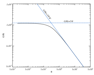
Figure 1: The dimensionless electron temperature distribution $G(\theta)=\theta/(\dot{\theta}t_{\rm c})$. The dashed and dotted lines are labelled to show how the distribution behaves in the non-relativistic and ultra-relativistic regimes respectively. i.e. $G(\theta)=5/4$ and $(3/8)\theta^{-1}$.

Figure 2: Electron energy distribution for 1T cooling cascade with $v_{\rm out}=0.1c$ and $T_{\rm sh}=2\times 10^{10}$K (solid curve). For comparison, a single temperature thermal electron distributions are also shown for $T=T_{\rm sh}$ and $T=T_{\rm IC}=2\times 10^{7}$K with the dotted and dash-dotted curves, respectively.

3 Resulting spectra for 1T and 2T shocks

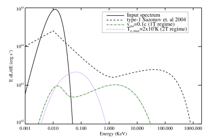
Figure 3: The Inverse Compton emission from shocked Ultra-Fast Outflows with $v_{\rm out}=0.1c$ in the 1T and 2T regimes (green dashed and purple dotted lines respectively). The primary soft photon spectrum from AGN, modelled as a simple black-body at $k_{B}T=3$eV, is also shown with a solid curve at low energies. The dashed curve shows a synthetic type 1 AGN spectrum from figure 4 of Sazonov et al. (2004).

Figure 3 shows the Inverse Compton spectra in both the 2T and 1T regimes, as labelled on the Figure. We assumed a SMBH of $M_{\rm bh}=10^{7}{\,{\rm M}_{\odot}}$ and outflow velocity of $v_{\rm out}=0.1c$. The input spectrum is modelled by a black-body of single temperature $k_{B}T=3$ eV and bolometric luminosity $L=L_{\rm bol}={L}_{\rm Edd}$. This simple model assumes that the UV luminosity of the innermost disc is absorbed and reprocessed into a cooler black-body spectrum (we remind the reader that we assume that the UFO shocks at “large” distances from the AGN, e.g., $R\sim 0.1-100$ pc). Also shown on the plots, for comparison, is a synthetic spectrum of a type 1 AGN as computed by Sazonov et al. (2004) normalised to the same bolometric luminosity. This last spectral component demonstrates that both 1T and 2T spectral components are actually comparable to the overall theoretical AGN spectra without UFOs; the 1T in the $\sim 2-10$ keV photon energy spectral window, whereas the 2T shock could be detectable in softer X-rays.

To explore the sensitivity of our results to model parameters, in Figure 4 we use observationally-motivated soft photon spectra from Sazonov et al. (2004) for energies below 0.1 keV, and we also consider two additional values for the outflow velocity, $v_{\rm out}/c=0.05$ and $0.2$. This figure also shows a synthetic type II (obscured AGN) spectrum from Sazonov et al. (2004), shown with the long-dash curve.

The figures demonstrate that at high enough outflow velocities, $v_{\rm out}\sim 0.2c$, the shocked UFOs produce power-law like spectra similar in their general appearance to that of a typical AGN. In fact, we made no attempt to fine tune any of the parameters of the King (2003) model to produce these spectra, so it is quite surprising that they are at all similar to the observed type I AGN spectra. In view of this fortuitous similarity of some of our IC spectra to the typical AGN X-ray spectra, one can enquire whether IC emission from $\sim pc$ scale shocks do actually contribute to the observed spectra.

Let us therefore compare the model predictions and X-ray AGN observations in some more detail:

1. Bolometric luminosity. Figures 3 and 4 are computed assuming 100% conversion of the UFO’s kinetic power in radiative luminosity, e.g., $L_{\rm IC}=L_{\rm k}$ (cf. equation 4) which is a fair assumption within the cooling radius, $R_{\rm IC}$, for the reverse shock (which is $\sim$ hundreds of pc for the 1T and just a few pc for the 2T models, respectively, see Zubovas & King, 2012b; Faucher-Giguere & Quataert, 2012). The ratio between the X-rays and the soft photon radiation in our model is thus $\sim(v_{\rm out}/2c)$, e.g., 0.05 for $v_{\rm out}=0.1c$, which is just a factor of a few smaller than it is in the typical observed AGN spectra. In terms of shear bolometric luminosity 1TIC and 2TIC are thus definitely observable.

   When the shock front propagated farther than $R_{\rm IC}$, the overall luminosity of the shock decreases. In the limit of extremely large $R_{\rm cd}$, where $R_{\rm cd}$ is the contact discontinuity radius, the primary outflow shocks at the radius $R_{\rm sw}\sim(1/5)R_{\rm cd}$ (see the text below equation 6 in Faucher-Giguere & Quataert, 2012). When $R_{\rm sw}\lower 2.15277pt\hbox{$\;\buildrel>\over{\sim}\;$}R_{\rm IC}$, the outflow is in the energy-conserving mode. We estimate that the IC luminosity would scale as $\propto R_{\rm IC}/R_{\rm sw}$ in this regime. In the intermediate regime, $R_{\rm sw}<R_{\rm IC}<R_{\rm cd}$, $L_{\rm IC}<L_{\rm k}$. A more detailed calculation is required in this regime to determine $L_{\rm IC}$ than has been performed here.

   In the model of King (2003), while the SMBH mass is below its critical $M_{\sigma}$ mass, the outflows stall in the inner galaxy, $R\lower 2.15277pt\hbox{$\;\buildrel<\over{\sim}\;$}R_{\rm ic}$. Once $M_{\rm bh}>M_{\sigma}$, however, the outflow quickly reaches $R\sim R_{\rm IC}$ and then switches over into the energy-conserving mode, which is far more efficient. Therefore, we would expect that the 1TIC shock emission should be a relatively widespread and relatively easily detectable feature in this scenario. In the 2TIC case, however, $R_{\rm IC}$ is just a few pc. Furthermore, since the outflow is much more likely to be in the energy conserving mode, even SMBH below the $M_{\sigma}$ mass may clear galaxies. We would expect shocks in this model spend most of the time in the regime $R_{\rm cd}\gg R_{\rm IC}$, being much dimmer than shown in figures 3 and 4. The 2TIC component is thus harder to detect for these reasons.

2. Variability. The IC shocks are very optically thin, so that the observer sees an integrated emission from the whole spherical shocked shell. Accordingly, the IC shell emission cannot vary faster than on time scale of $R_{\rm cd}/c\sim 30$ years $R_{\rm cd}/(10$ pc). The shock travel time is even longer by the factor $c/v_{\rm out}\sim 10$. This therefore predicts that IC shock emission must be essentially a steady-state component in X-ray spectra of AGN. In contrast, observed X-ray spectra of AGN vary strongly on all sorts of time scales, from the duration of human history of X-ray observations, e.g., tens of years, to days and fractions of hour (e.g., Vaughan et al., 2003). This rapid variability is taken to be a direct evidence that observed X-rays must be emitted from very close in to the last stable orbit around SMBHs.

3. No molecular torus obscuration in X-rays. Nuclear emission of AGN, from optical/UV to X-rays, is partially absorbed in “molecular torii” (Antonucci, 1993) of $\sim$ pc scale (Tristram et al., 2009). This obscuration produces the very steep absorption trough in soft X-rays seen in type II AGN as compared with the type I sources (cf. long-dashed versus dashed curves in Fig.4). If a sizeable fraction of X-ray continuum from AGN were arising from the IC shocks on larger scales, then that emission would not show any signatures of nuclear X-ray absorption. While Gallo et al. (2013) reports one such “strange” AGN, it is also a very rapidly varying one (cf. their figs. 9 and 10), which again rule out the 1TIC model. There are also examples when soft X-ray absorption varied strongly on short time scales (e.g., Puccetti et al., 2007), indicating that X-ray emission region is as small as $10^{-4}$ pc.

4. No reflection component. Compton down scattering and soft-X-ray absorption by circum-nuclear gas produces the reflection component or “Compton hump” observed in many AGN at $\sim 30$ KeV (Guilbert & Rees, 1988; Pounds et al., 1990). In addition, the fluorescent Fe K-$\alpha$ line emission is associated with the same process and is frequently detected in X-ray spectra of AG (Nandra & Pounds, 1994). Since the shocks that we study occur on large scales, the IC emission would likely impact optically thin cold gas and thus result in much weaker X-ray reflection and Fe K-$\alpha$ line emission than actually observed.

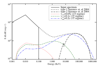
Figure 4: The Inverse Compton emission from shocked Ultra-Fast Outflows with $v_{\rm out}=0.05$, $0.1$ and $0.2$c (red dotted, green dash-dotted and blue dash-double dotted respectively) in the 1T regime only. In contrast with fig. 3 the primary soft photon spectrum from the AGN is modelled by the the $1-100$eV region of the type 1 AGN spectrum from figure 4 Sazonov et al. (2004). The black dashed and long-dashed curves shows synthetic type 1 and type 2 AGN spectra from figure 4 of Sazonov et al. (2004) respectively.

Given these points, we can completely rule out the most extreme assumption that the X-ray emission of AGN is due to UFO shocks alone. The next question to ask is whether having the 1TIC or 2TIC emission from the UFOs in addition to the “nuclear” X-ray corona emission of AGN (Haardt & Maraschi, 1993) would be consistent with the present data. To address this, we calculate the 1TIC and 2TIC emission as for figure 4, but now including the part of the Sazonov et al. (2004) spectrum above 0.1 keV, which means that we now also include IC scattering of the higher energy radiation from AGN in the UFO shocks (rather than only the disc emission). The resulting spectra are shown in Figure 5.

We see that the 1TIC spectra would be ruled out in deeply absorbed type II AGN spectra, because the 1TIC component would be very obvious in these sources below a few keV. The 2TIC component, on the other hand, would not be so prominent except in very soft X-rays where interstellar absorption is significant. We therefore preliminarily suggest that X-ray emission from 1T UFO shocks may contradict the data for type II AGN, whereas 2TIC spectra would probably be comfortably within the observational limits.

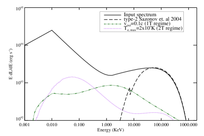
Figure 5: Same as figure 3, but now assuming that the AGN spectrum in exactly equal to the model of Sazonov et al. (2004). Again we show the case where $v_{\rm out}=0.1c$ in the 1T and 2T regimes (green dashed and purple dotted lines respectively).

4 Discussion and Conclusions

We calculated X-ray spectra of 1T and 2T Inverse Compton shocks resulting from ultra-fast outflows from AGN colliding with the ambient host galaxy medium. We concluded that 1TIC spectra could be detectable in AGN spectra and distinguisheable from “typical” AGN spectra actually observed by absence of rapid variability, Compton reflection and Fe K-$\alpha$ lines. This disfavours 1T models for AGN feedback in our opinion. We must nevertheless caution that the quoted typical observed AGN spectra and properties may be dominated by local objects that are simply not bright enough to produce a significant kinetic power in outflows, which our model here assumed. We therefore urge X-ray observers to search for the un-absorbed and quasi-steady emission components presented in our paper in order to clarify the situation further.

It is interesting to note that the 2T Inverse Compton emission (2TIC) comes out mainly in the soft X-rays where it is far less conspicuous as this region is usually strongly absorbed by a cold intervening absorber. In fact, it is possible that 2TIC emission component calculated here does contribute to the observed “soft X-ray excess” feature found at softer X-ray energies ($<1$ KeV) but not yet understood (Gierliński & Done, 2004; Ross & Fabian, 2005; Crummy et al., 2006; Scott et al., 2012). The 2T spectral component in figure 3 is close to the observed shape of the soft excess and would provide a soft excess that is independent of the X-ray continuum, a requirement suggested by e.g. Rivers et al. (2012). The observed soft excess does not vary in spectral position over a large range of AGN luminosities (Walter & Fink, 1993; Gierliński & Done, 2004; Porquet et al., 2004). The 2TIC model may account for this as well since figure 2. of Faucher-Giguere & Quataert (2012) shows that $T_{\rm{eq}}$ is quite insensitive to the exact value of the outflow velocity. Finally, the 2TIC emission would exhibit little time variability. Uttley et al. (2003); Pounds & Vaughan (2011) reported a quasi-constant soft X-ray component in NGC 4051 which could only be seen during periods of low (medium energy) X-ray flux, which is qualitatively consistent with the 2TIC shock scenario.

Therefore, we conclude that general facts from present X-ray observations of AGN not only disfavour 1TIC component over 2TIC component but may actually hint on the presence of a 2TIC one in the observed spectra.

Whether the electrons thermally decouple from hot protons is vitally important for the problem of AGN feedback on their host galaxies. Because of their far larger mass, the ions carry virtually all the kinetic energy of the outflow. At the same time, ions are very inefficient in radiating their energy away compared with the electrons. In the 1T model, the electrons are able to sap away most of the shocked ions energy and therefore the AGN feedback is radiative, that is, momentum-driven, inside the cooling radius (King, 2003). In this scenario only the momentum of the outflow affects the host galaxy’s gas. In the 2T scenario, the outflow is non-radiative, so that the ions retain most of their energy. The AGN feedback is thus even more important for their host galaxies in this energy-driven regime (Zubovas & King, 2012a; Faucher-Giguere & Quataert, 2012).

If the outflows are indeed in the 2T mode, then one immediate implication concerns the recently discovered positive AGN feedback on their host galaxies. Well resolved numerical simulations of Nayakshin & Zubovas (2012); Zubovas et al. (2013b) show that ambient gas, when compressed in the forward shock (to clarify, the shock we studied here is the reverse one driven in the primary UFO), can cool rapidly in the gas-rich host galaxies. The nearly isothermal outer shock is gravitationally unstable and can form stars. In addition, Zubovas et al. (2013a) argue that galactic gas discs can also be pressurised very strongly by the AGN-driven bubble. In these cases AGN actually have a positive – accelerating – influence on the star formation rate in the host galaxy. Within the 1T formalism, the AGN-triggered starbursts occur outside $R_{\rm IC}\sim$ hundreds of pc only (Zubovas et al., 2013a). If outflows are 2T then AGN can accelerate or trigger star bursts even in the nuclear regions of their hosts.

References

- Antonucci (1993) Antonucci R., 1993, ARA&A, 31, 473
- Ciotti & Ostriker (2007) Ciotti L., Ostriker J. P., 2007, ApJ, 665, 1038
- Crummy et al. (2006) Crummy J., Fabian A. C., Gallo L., Ross R. R., 2006, MNRAS, 365, 1067
- Faucher-Giguere & Quataert (2012) Faucher-Giguere C.-A., Quataert E., 2012, ArXiv e-prints
- Feruglio et al. (2010) Feruglio C., Maiolino R., Piconcelli E., et al., 2010, A&A, 518, L155
- Gallo et al. (2013) Gallo L. C., MacMackin C., Vasudevan R., Cackett E. M., Fabian A. C., Panessa F., 2013, ArXiv e-prints
- Gierliński & Done (2004) Gierliński M., Done C., 2004, MNRAS, 349, L7
- Guilbert & Rees (1988) Guilbert P. W., Rees M. J., 1988, MNRAS, 233, 475
- Haardt & Maraschi (1993) Haardt F., Maraschi L., 1993, ApJ, 413, 507
- King (2003) King A., 2003, ApJL, 596, L27
- King (2010) King A. R., 2010, MNRAS, 402, 1516
- Liu et al. (2013) Liu G., Zakamska N. L., Greene J. E., Nesvadba N. P. H., Liu X., 2013, ArXiv e-prints
- Nagirner & Poutanen (1994) Nagirner D. I., Poutanen J., 1994, Single Compton scattering
- Nandra & Pounds (1994) Nandra K., Pounds K. A., 1994, MNRAS, 268, 405
- Nayakshin & Melia (1998) Nayakshin S., Melia F., 1998, ApJS, 114, 269
- Nayakshin & Zubovas (2012) Nayakshin S., Zubovas K., 2012, MNRAS, 427, 372
- Porquet et al. (2004) Porquet D., Reeves J. N., O’Brien P., Brinkmann W., 2004, A&A, 422, 85
- Pounds et al. (2003a) Pounds K. A., King A. R., Page K. L., O’Brien P. T., 2003a, MNRAS, 346, 1025
- Pounds et al. (1990) Pounds K. A., Nandra K., Stewart G. C., George I. M., Fabian A. C., 1990, Nature, 344, 132
- Pounds et al. (2003b) Pounds K. A., Reeves J. N., King A. R., Page K. L., O’Brien P. T., Turner M. J. L., 2003b, MNRAS, 345, 705
- Pounds & Vaughan (2011) Pounds K. A., Vaughan S., 2011, MNRAS, 413, 1251
- Puccetti et al. (2007) Puccetti S., Fiore F., Risaliti G., Capalbi M., Elvis M., Nicastro F., 2007, MNRAS, 377, 607
- Quataert (1998) Quataert E., 1998, ApJ, 500, 978
- Rivers et al. (2012) Rivers E., Markowitz A., Duro R., Rothschild R., 2012, ApJ, 759, 63
- Ross & Fabian (2005) Ross R. R., Fabian A. C., 2005, MNRAS, 358, 211
- Rupke & Veilleux (2011) Rupke D. S. N., Veilleux S., 2011, ApJL, 729, L27
- Rybicki & Lightman (1986) Rybicki G. B., Lightman A. P., 1986, Radiative Processes in Astrophysics, Radiative Processes in Astrophysics, by George B. Rybicki, Alan P. Lightman, pp. 400. ISBN 0-471-82759-2. Wiley-VCH , June 1986.
- Sazonov et al. (2004) Sazonov S. Y., Ostriker J. P., Sunyaev R. A., 2004, MNRAS, 347, 144
- Scott et al. (2012) Scott A. E., Stewart G. C., Mateos S., 2012, MNRAS, 423, 2633
- Shakura & Sunyaev (1973) Shakura N. I., Sunyaev R. A., 1973, A&A, 24, 337
- Stepney (1983) Stepney S., 1983, MNRAS, 202, 467
- Sturm et al. (2011) Sturm E., González-Alfonso E., Veilleux S., et al., 2011, ApJL, 733, L16
- Tombesi et al. (2010a) Tombesi F., Cappi M., Reeves J. N., et al., 2010a, A&A, 521, A57+
- Tombesi et al. (2010b) Tombesi F., Sambruna R. M., Reeves J. N., et al., 2010b, ApJ, 719, 700
- Tristram et al. (2009) Tristram K. R. W., Raban D., Meisenheimer K., et al., 2009, A&A, 502, 67
- Uttley et al. (2003) Uttley P., Fruscione A., McHardy I., Lamer G., 2003, ApJ, 595, 656
- Vaughan et al. (2003) Vaughan S., Edelson R., Warwick R. S., Uttley P., 2003, MNRAS, 345, 1271
- Walter & Fink (1993) Walter R., Fink H. H., 1993, A&A, 274, 105
- Weaver et al. (1977) Weaver R., McCray R., Castor J., Shapiro P., Moore R., 1977, ApJ, 218, 377
- Zubovas & King (2012a) Zubovas K., King A., 2012a, ApJL, 745, L34
- Zubovas & King (2012b) Zubovas K., King A. R., 2012b, ArXiv e-prints
- Zubovas et al. (2013a) Zubovas K., Nayakshin S., King A., Wilkinson M., 2013a, ArXiv e-prints
- Zubovas et al. (2013b) Zubovas K., Nayakshin S., Sazonov S., Sunyaev R., 2013b, MNRAS, 431, 793