Are giant tornadoes the legs of solar prominences?

Abstract

Observations in the 171 Å channel of the Atmospheric Imaging Assembly of the space-borne Solar Dynamics Observatory show tornadoes-like features in the atmosphere of the Sun. These giant tornadoes appear as dark, elongated and apparently rotating structures in front of a brighter background. This phenomenon is thought to be produced by rotating magnetic field structures that extend throughout the atmosphere. We characterize giant tornadoes through a statistical analysis of properties like spatial distribution, lifetimes, and sizes. A total number of 201 giant tornadoes are detected in a period of 25 days, suggesting that on average about 30 events are present across the whole Sun at a time close to solar maximum. Most tornadoes appear in groups and seem to form the legs of prominences, thus serving as plasma sources/sinks. Additional H$\alpha$ observations with the Swedish 1-m Solar Telescope imply that giant tornadoes rotate as a structure although clearly exhibiting a thread-like structure. We observe tornado groups that grow prior to the eruption of the connected prominence. The rotation of the tornadoes may progressively twist the magnetic structure of the prominence until it becomes unstable and erupts. Finally, we investigate the potential relation of giant tornadoes to other phenomena, which may also be produced by rotating magnetic field structures. A comparison to cyclones, magnetic tornadoes and spicules implies that such events are more abundant and short-lived the smaller they are. This comparison might help to construct a power law for the effective atmospheric heating contribution as function of spatial scale.

1. Introduction

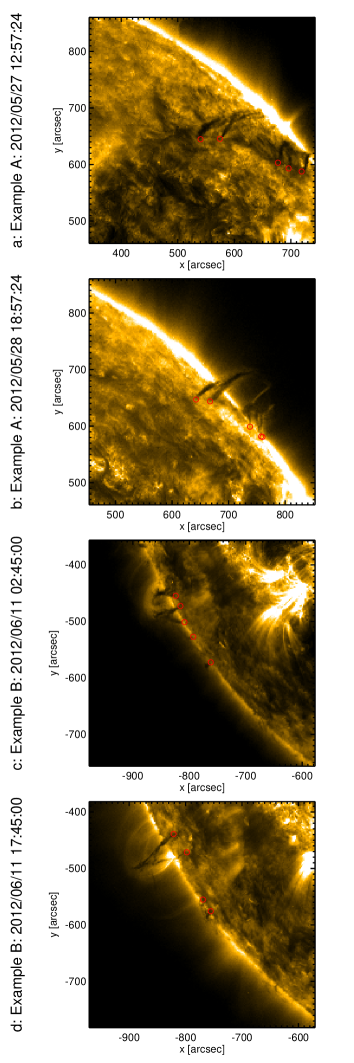
Figure 1.— Intensity images from the AIA channel at 171 Å showing examples of tornado groups. The group in the two upper panels consists of 5 clear tornadoes at different times, whereas the other group in the two lower panels has at least 4-5 tornadoes. The bottom panel shows the latter group shortly before eruption. The tornado footpoints are marked by small red dots.

The term ‘tornado’ has been used repeatedly for phenomena on the Sun, in particular in connection with prominences (Pettit 1932), although the physical processes behind their formation are very different from those responsible for terrestrial tornadoes. ’Tornado prominences’ have been studied numerous times with spectroscopic observations dating back to 1868 (cf. Zöllner 1869; Pettit 1950). Tandberg-Hansen refers to tornadoes as vertically aligned, helical structures, which are connected to solar prominences (see Chap. 10 in Bruzek & Durrant 1977). The terms prominence and filament are used synonymously here since they describe the same phenomenon seen on-disk and at the limb, respectively (see, e.g., Zirker 1989; Engvold 1998; Martin 1998; Mackay et al. 2010; Joshi et al. 2013, and references therein for overview articles). In the 1990s, observations of solar tornadoes, to which we refer to as ‘giant tornadoes’ hereafter, have been made by Pike & Mason (1998) with the Coronal Diagnostic Spectrometer (CDS, Harrison et al. 1995) onboard the Solar and Heliospheric Observatory (SOHO, Domingo et al. 1995). These observations suggest that rotation may play an important role for the dynamics of the solar transition region (see also Pike & Harrison 1997; Banerjee et al. 2000). More recently, this phenomenon was observed in detail with the Atmospheric Imaging Assembly (AIA) onboard the Solar Dynamics Observatory (SDO, Lemen et al. 2012). For instance, Li et al. (2012) detected plasma that moves along spiral paths with an apparent rotation that lasted for more than three hours. Different types of rotation of a filament are also observed by Su & van Ballegooijen (2013). It is likely that giant tornadoes – at least the majority of them – are the vertical legs of prominences and filaments. Recently, Su et al. (2012) suggested that barbs are another observational imprint of giant tornadoes (see also Li et al. 2012). Barbs are observed in the H$\alpha$ line and are known to be rooted in the photosphere and to connect to the horizontal ’spine’ of a filament in the upper atmosphere (e.g., Zirker et al. 1998; Martin 1998; Li & Zhang 2013, and references therein). Despite their apparent motion, it is not clear yet (see, e.g., Panasenco et al. 2013) if giant tornadoes truly rotate as entities although Orozco Suárez et al. (2012) provided support for this hypothesis. They measured Doppler shifts of $\pm 6$ km s^-1 at the opposite sides of legs of a quiescent hedgerow prominence, which they interpret as rotation of the structure around an axis vertical to the solar surface. Panesar et al. (2013) suggest that tornadoes could be caused by the helical magnetic field of a prominence in response to the expansion of the corresponding cavity, whereas Su et al. (2012) propose that giant tornadoes can be explained as rotating magnetic structures driven by underlying photospheric vortex flows. The latter explanation matches the mechanism that has recently been found for so-called magnetic tornadoes by Wedemeyer-Böhm et al. (2012) although these events, which have only been observed on-disk so far, seem to be smaller than the prominence-related giant tornadoes discussed here. Hence, it is not clear yet if the small-scale tornadoes and the giant tornadoes are connected but the physical processes behind might be similar to some extent. The observations and accompanying 3D numerical simulations by Wedemeyer-Böhm et al. (2012) clearly show that magnetic tornadoes are caused by vortex flows in the photosphere, which force the footpoints of magnetic field structures to rotate. These events are observed with the Swedish 1-m Solar Telescope (SST, Scharmer et al. 2003a) as ‘chromospheric swirls’ in image sequences in the core of the Ca II 854.2 nm line (Wedemeyer-Böhm & Rouppe van der Voort 2009) but also have an imprint in AIA/SDO images.

Here, we present a systematic analysis of giant tornadoes as they appear in SDO AIA 171 Å images regarding their spatial distribution and statistics of their sizes and lifetimes. We also compare the AIA 171 Å tornadoes to the corresponding imprints in other AIA channels, magnetograms, and high-resolution SST observations. Based on this data, we provide support for the following hypotheses: (i) Giant tornadoes are an integral part of solar prominences. (ii) Giant tornadoes serve as sources and sinks of the mass flow of prominence material. (iii) They may inject helicity into the connected prominence, which can lead to its eruption. The observations are described in Sect. 2, followed by the results in Sect. 3, discussion in Sect. 4 and conclusions in Sect. 5, respectively.

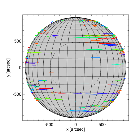
Figure 2.— Distribution of all detected events on the full disk of the Sun. The tracks of all events are plotted although not all of them exist at the same time. The central region appears to be void due to projection effects that make it difficult to detect the tornado-like structure close to disk-centre. The two open circles mark the positions of the detailed SST observations.

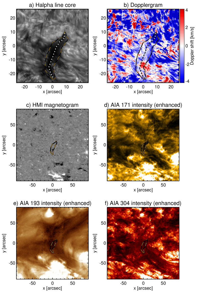
Figure 3.— Observation of an on-disk tornado. a) H$\alpha$ line core image taken with SST/CRISP and b) the corresponding Dopplergram. The color range of the Dopplergram is limited to $\pm 4$ km s^-1, while the full range is $[-14.7,11.8]$ km s^-1. The yellow-black dashed line outline the tornado, whereas the black-white dotted line represents the centerline. The panels below display SDO images for a larger FOV: c) HMI magnetogram, d) AIA 171, e) AIA 193, and f) AIA 304. The dotted boxes mark the SST FOV.

2. Observations and data reduction

We analyze images taken with AIA/SDO and systematically detect ‘giant tornadoes’ throughout the period from May 27^th, 2012 to June 21^st, 2012. It is important to note that this period corresponds to a time of high solar activity. This period is long enough to cover roughly one solar revolution and thus results in a statistically significant sample. The data channel at 171 Å is used for the initial detection with JHelioviewer and for a determination of positions and lifetimes. Next, the AIA images for the whole period are downloaded with a cadence of 1 hour and post-processed with standard SolarSoft routines to level 1.5 data. It includes dark current correction, flat-fielding, hot pixel correction and de-spiking, as well as deconvolution with a point spread function, de-rotation and scale correction.

Those events that are already present in the first time step or are still present in the last timestep are followed beyond the analyzed period in order to reliably determine their lifetime. The positions and the shapes of all events are evaluated throughout the time series. For selected events, 193 Å, 211 Å, and 304 Å images are investigated, too. Corresponding magnetograms from the Helioseismic and Magnetic Imager (HMI, Scherrer et al. 2012) onboard SDO are analysed in order to determine the photospheric magnetic field topology close to the tornadoes. Examples of tornadoes are shown in Fig. 1. They appear as dark and elongated features in front of a brighter background with a narrow footpoint and a more diffuse top. Time-series of the dark features reveal apparent rotation. This signature is pronounced for the majority (81.5 %) of all cases but can be more subtle for other examples, which we hereafter refer to as less confidently identified. In addition, daily full-disk H$\alpha$ images from the Big Bear Solar Observatory (BBSO) are obtained from the Virtual Solar Observatory (Hill et al. 2004) for the whole observation period and searched for prominences.

Two of the tornadoes, which are identified in our sample, have also been observed with the SST on June 8th, 2012. One event was observed on-disk, whereas the other was located above the limb (see open circles in Fig. 2). The on-disk event was observed at 9:58 UT at $x=-720$″, $y=-342$″ and the off-limb event at 12:24 UT at $x=894$″, $y=374$″. The CRISP instrument (Scharmer et al. 2008) was used to scan through the H$\alpha$ line with a fine wavelength sampling of 86 mÅ (39 line positions for the on-disk event, 33 line positions for the off-limb event). The seeing was very variable during the time of observation which inhibited extensive temporal coverage. Here we restrict to the analysis of the best scans. For the on-disk event, high-spatial resolution was achieved for the best scan with the aid of the SST adaptive optics system (Scharmer et al. 2003b) and Multi-Object Multi-Frame Blind Deconvolution image restoration (van Noort et al. 2005). The pixel scale of these frames is 0.059″. For more information on the optical set-up and processing, we refer to, e.g., Sekse et al. (2012). For the off-limb event, the adaptive optics system could not actively compensate for seeing and we restrict the image post-processing to the standard dark current and flatfield corrections. A pixel binning of $2\,\times\,2$ has been applied in this case. The quality of the selected line scans was nevertheless sufficient to construct reliable Dopplergrams. The nature of the spectral line profiles, which change from absorption profiles on-disk to emission profiles off-limb, is taken into account for the determination of the Doppler shifts. The Doppler shifts for flat and noisy profiles, which are found in off-limb areas outside the tornado, are set to zero. Corresponding AIA images for the same time and locations are rotated and aligned with the SST observations. For inspection and exploration of the SST data we used the widget-based analysis tool CRISPEX (Vissers & Rouppe van der Voort 2012), which allows for efficient exploration of multi-dimensional datasets. See Sects. 3.1 and 3.2 for the results of the analysis.

3. Analysis of tornado properties

3.1. AIA and SST observations of an on-disk tornado

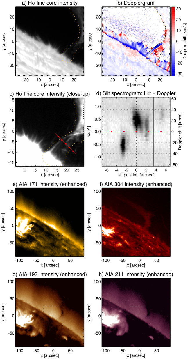
Figure 4.— Off-limb observation of a tornado. a) H$\alpha$ line core image taken with the SST on June 8th, 2012, and b) the corresponding Dopplergram. c) Enhanced H$\alpha$ line core intensity for a close-up of the tornado base with an artificial slit (red line with markers every 2.5″). d) Slit spectrogram, i.e., reversed H$\alpha$ intensity as function of position along the slit and wavelength. The black vertical lines mark the tornado boundaries. The panels below show SDO/AIA images for a slightly larger FOV: e) 171 Å, f) 304 Å, g) 193 Å, h) 211 Å. The FOV from the top row is marked as dotted box.

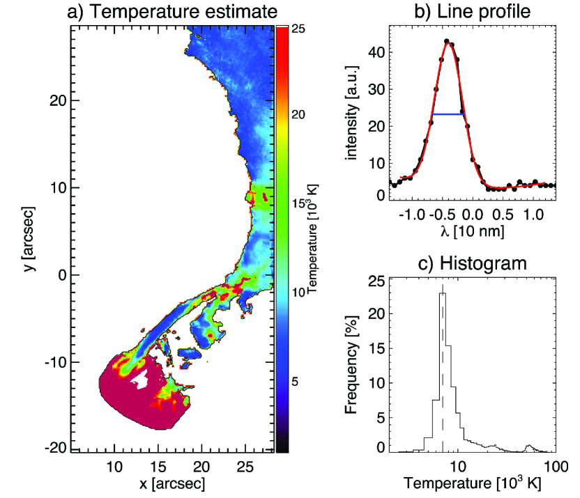
Figure 5.— Temperature estimate for the off-limb tornado. a) Derived temperature in a close-up region. Pixels are white if no value was determined and pink if the value exceeds 20 000 K. b) Intensity profile at $x=16.1\arcsec,y=-5.3\arcsec$ (black dots) with Gaussian fit (red) and FWHM (horizontal blue line), c) Histogram of the temperature values for all pixels that are not white in panel a.

The on-disk tornado is clearly visible in the H$\alpha$ line core images and also the AIA 171 Å image, whereas there is only a subtle imprint in the other AIA channels (see Fig. 3). Please refer to Anzer & Heinzel (2005) for a detailed account on the formation of the intensity at 171 Å. The tornado in the H$\alpha$ image is slightly bent and has a length of 37″ measured along the centerline. The dark structure is less than 4.4″ wide with its middle part having a typical width of $\sim 3.3$″. The imprint in the 171 Å image has a similar width, whereas the length is determined to only $\sim 31$″ because the thinnest parts are not resolved with SDO. The dark thin threads to the left of the tornado outline the overlying filament, which is visible in the 193 Å and 304 Å images. The filament lies presumably above the tornado, which is rooted in a photospheric footpoint and connects to the filament threads. The footpoint, which we do not observe directly, is likely to be located close to the end of the H$\alpha$ signature (at $x=9.2$″, $y=9.7$″ in Fig. 3a). The HMI magnetogram shows no clear photospheric footpoint of the tornado. There is only one single magnetic point co-located with the tornado but it is not clear if this photospheric feature is connected to the chromospheric tornado signature as seen in H$\alpha$ (see Fig. 3c).

The spectral line profiles at positions inside the on-disk tornado have only small Doppler shifts, are mostly symmetric and have a lower line core intensity than the background. Many threads in the filament spine, which thus are not part of the tornado itself, can also be discerned in the Doppler map as a pattern of stripes almost perpendicular to the tornado axis. This imprint implies that the line core intensity has strong contributions from the filament threads, whereas the tornado only causes moderate additional absorption. We conclude that the strong contributions of the filament render these observations unsuitable for measuring velocities that could be attributed unambiguously to the tornado.

3.2. AIA and SST observations of an off-limb tornado

The SST observations of the off-limb tornado provide a clearer picture (see Fig. 4a-d). The corresponding AIA 171 Å image (see Fig. 4e) indeed shows that the SST observations coincide with a detected tornado event. Although the lower part of the tornado is difficult to see for this instance in time in the AIA 171 Å image, a dark absorption feature can be outlined. There is an indication of a cavity above the tornado, like for the event observed by Li et al. (2012). The 304 Å AIA image in Fig. 4f reveals a prominence bending sidewards from the tornado, roughly coinciding with the observed cavity. The 304 Å image further reveals a narrow base for the tornado, which extends $\sim$ 30″above the solar limb before it bends sidewards towards the pole. The field of view (FOV) of the SST observations includes the tornado base. The H$\alpha$ line core images (see Fig. 4a,c) exhibit thin elongated threads that extend almost vertically above the limb before bending sidewards, too. These threads give the impression of a helical structure, while the lateral continuation resembles a ’smoke-like streamer’ – features of ’tornado prominences’ that have been described for a long time (e.g. Pettit 1950). The best visible thread, which is rooted at the left side of the tornado base, has a width of 0.4″ - 0.5″. This width is close to the limit of what can be resolved in this data set in view of the moderate seeing conditions. The lower parts of the thread coincide with an elongated region with a strong blue shift in the SST Doppler map in Fig. 4b, although the blue-shifted region has a width of 1.6″ - 1.8″ and is thus much wider than the line core thread. The blue shifts are on the order of $-20$ km s^-1 to $-30$ km s^-1. The remaining tornado base exhibits strong red shifts mostly between $10$ km s^-1 and $30$ km s^-1. Both regions extend vertically $\sim$ 12″. Above, mostly only weak shifts are observed. The Doppler signal in the lowermost part of the tornado is obscured by plasma in the foreground. The whole tornado base, which is both visible in the Dopplergram and in the 304 Å AIA image, has a width between 6″ and 8″, measured from the outer edges of the Doppler shifted regions. The spectrogram in Fig. 4d) shows the H$\alpha$ intensity along the artificial slit, which is marked in panel c. Dark shades mark the H$\alpha$ emission peak and thus allow for estimating the Doppler shift along the slit. Along the slit inside the tornado (between the vertical black lines), the Doppler shift changes from about $-20$ km s^-1 on one side to about $+20$ km s^-1 on the other side. At this speed, an uniformly rotating cylinder with a width of 7″ would revolve in $\sim 14$ min. On the other hand, we expect a more complex rotation pattern given the fine-structure, which is clearly visible in the close-up of the line core image in Fig. 4c and also in the apparent gap in the middle of the slit in Fig. 4d. The tornado structure may rotate as a whole but only the thin threads, which compose the tornado base, provide tracers of the rotation.

The tornado structure is also visible in other AIA channels, which differ in the formation and the contribution to the intensity in the pass-bands and – in approximation – map plasma at different effective temperature. With the exception of the 304 Å channel in which the tornado appears in emission, all other AIA channels show the tornado as a dark absorption-like structure. All analysed channels show a tornado structure that is narrow at the base, funnels out above and continues sideways into the prominence. This lateral continuation is most visible in the 304 Å channel but appears only as a very faint streak in the 171, 193, and 211. The imprint in the 304 Å image has an apparent total length of 140-150″, measured from the footpoint at the limb to the outermost faint end. This imprint has a width of $\sim$8″at the base, 14-15″ near the bend-over point and 14-20″ in the prominence part. The thin thread that is visible in emission in the H$\alpha$ line core image is also visible as a dark feature in 193 Å next to another thread that is better visible in 193 Å  than in H$\alpha$. The 211 Å images are very similar. We measure widths for these threads, which are on the order of the pixelscale ($\sim$0.6″) of SDO. The tornado structure funnels out above the base and has widths of 5 - 8″ close to the bend-over point. This width agrees with the characteristic value of 5.7″, which is determined based on the 171 Å signature. The corresponding length is 20″.

The Doppler shifts with opposite sign at the edges of the tornado base strongly imply that the tornado structure rotates. In that picture, the plasma on one side moves towards the observer and the plasma on the other side of the tornado away from the observer. The observation that the red-shifted area is larger than the blue-shifted part speaks against a uniformly rotating cylinder but rather implies a more complex geometry like, e.g., a elliptical cross-section or a threaded sub-structure. In this regard, it should be emphasized that the observations at the limb are very challenging and important details may not have been resolved so far. The Doppler signature can nevertheless be interpreted as a rotation, while the amplitudes of the Doppler velocities have to be analysed with more caution. It cannot be completely ruled out that we observe two regions that appear close in projection but actually move away from each other at high speed. It seems however questionable that the tornado structure could remain stable for the observed duration in this case. Another possible explanation is that the Doppler signals are due to counter-streaming flows like they have been observed by Zirker et al. (1998) in barbs and along the spine of a prominence. They measure plasma speeds of $5-20$ km s^-1, which is in the same range as the Doppler shifts found in this work. Although this possibility certainly cannot be ruled out on basis of the available data, the rotation of the tornado base seems to be the more likely explanation in view of the apparent motions in SDO image series. This conclusion is in line with the results by Orozco Suárez et al. (2012) for the legs of a quiescent hedgerow prominence, for which they determine opposite Doppler shifts of $\pm 6$ km s^-1 at the opposite sides. This interpretation also agrees with the findings concerning solar tornadoes presented by Su et al. (2012), who report on rotation speeds of $5-10$ km s^-1, and Wedemeyer-Böhm et al. (2012).

By calculating the width of the H$\alpha$ line profile we can further determine upper limits for the plasma temperature inside the tornado. At a position of $x=16.1\arcsec,y=-5.3\arcsec$ in the left blue-shifted thread, we observe a typical emission profile, which is shown in Fig. 5b. We correct the profile for straylight contributions by subtracting the intensity offset as determined from the outer wavelength positions and then fit the profile with a Gaussian. The line width $\Xi$ is then derived as FWHM of the Gaussian. The corresponding gas temperature of the emitting region in the tornado can be estimated according to Antolin & Rouppe van der Voort (2012, see their Eq. 7) as

$$T=\frac{1}{16\,\ln 2}\ \frac{c^{2}\,m_{\mathrm{H}}}{k_{\mathrm{B}}}\ \left(\frac{\Xi}{\lambda_{0}}\right)^{2}\qquad,$$ (1)

where we ignored the microturbulence. Here we choose to ignore the microturbulence in order to obtain upper limits for the temperature. The resulting temperature values span a range from 4 000 K to 88 000 K, although the temperature is typically below 25 000 K in the depicted part of the tornado (see Fig. 5a). The corresponding histogram in panel c exhibits a maximum at 7 000 K. In the left blue-shifted thread, we find temperatures between 5 000 K and 10 000 K.

3.3. Abundance and spatial distribution.

A total number of 201 tornadoes is detected in the time period of 25 days. On average there are 11.2 events present at the same time although the total number varies between 2 and 25 (see Fig. 6). Due to projection effects tornadoes are difficult to detect in the central parts of the solar disk inside a half solar radius ($R_{\mathrm{c}}=\frac{1}{2}\,R_{\odot}$, see dotted circle in Fig. 2). The numbers should be multiplied by a factor to account for the central part and the backside of the Sun. We derive correction factors between $4/\sqrt{3}$ (when accounting for the observed area fraction on a spherical surface) and $\text@frac{8}{3}$ when using the area fraction on the projected disk instead. With the latter, we estimate that on average there are about 30 tornadoes present on the Sun at the same time during the analysed period. The numbers are reduced to 9.7 events at the same time and about 26 over the whole surface if only the confidently detected events are considered. The variation of this number with the solar cycle has to be investigated in a future study.

The distribution of the tornado events over latitude is shown in Fig. 7. They appear mostly at mid-latitudes, whereas there are essentially no giant tornadoes present close to the solar equator and the poles. This distribution resembles that of the activity belt, which suggests a close connection to strong magnetic field concentrations.

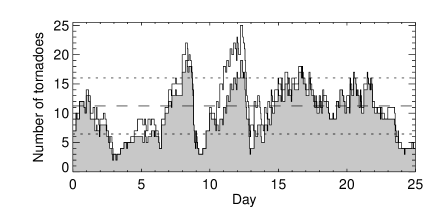
Figure 6.— Total number of tornadoes visible in AIA 171 Å images as function of time. The grey-shades area represents the number of confidently detected tornadoes whereas the white areas on top also account for less confidently detected events. The horizontal lines represent the average (dashed) plus/minus standard deviation (dotted) for all events.

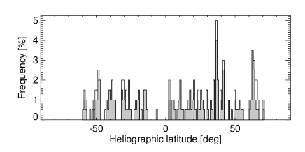
Figure 7.— Distribution of giant tornadoes over heliographic latitude: All events (white) and confident examples only (grey).

Based on the BBSO full-disk H$\alpha$ images, we find that 91 % of all detected tornadoes are co-located with filaments or prominences. The remaining apparently ’isolated’ tornadoes are less confident detections, except for two cases which are only seen shortly before disappearing at the west limb. It is therefore plausible to assume that all giant tornadoes are part of a filament. The majority of the tornadoes in our data set therefore appear in groups located along filament channels. The analysis of HMI magnetograms reveals that these ’tornado alleys’ are related to polarity inversion lines (see Sect. 3.6). The groups consist typically of three to seven coexistent tornadoes. Additional tornadoes can appear and disappear during the lifetime of a group, resulting in up to 15 tornado detections for some groups. We find a continuous spectrum of distances between coexistent tornadoes within the same group, where 83 % of all tornadoes are located 80″ or less and 71 % less than 50″ from a neighbouring group member, respectively. In many cases, the tornado groups are co-located with ‘barbs’ in connection with a filament/prominence (see Sect. 4).

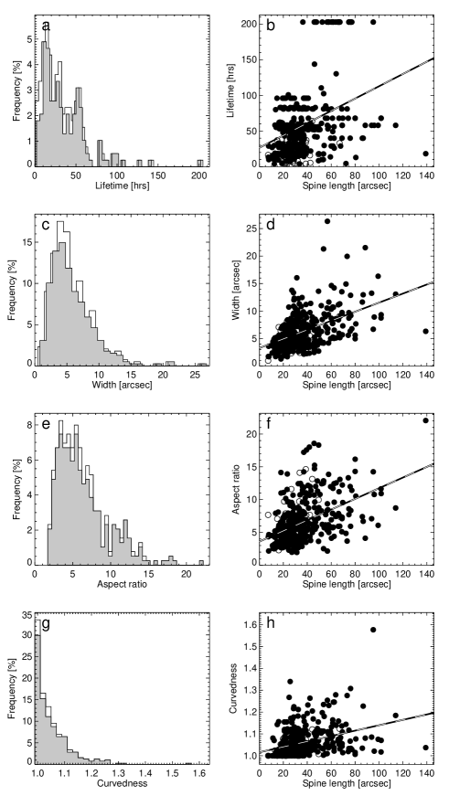
Figure 8.— Statistics of tornado lifetime (a,b), characteristic width (c,d), aspect ratio (e,f), and curvedness (g,h). The left column shows the histogram for all measurements (white) and for the confident examples (grey). Each property is plotted against the tornado centralline length (right column), where confident examples are represented by filled circles and less confident ones by open circles. A linear regression line is plotted to illustrate the trend for each property.

3.4. Apparent tornado lifetimes in 171 Å images

The lifetimes of all confidently detected tornadoes range from only one hour to 202 hours. Events that existed already at the beginning of the analyzed period and events that lasted longer than the period have been tracked beyond the period and the lifetimes have been determined correspondingly. The histogram of the lifetimes (Fig. 8a) reveals that most tornadoes live for less than 60 hours. The average lifetime is 35 hours with a large standard deviation of 27 hours although the latter is reduced to 20 hours when excluding the less confidently detected examples. Only 15 events (7.5 %) last for more than 3 days and only 8  (4 %) for more than 4 days, respectively. Only 5 % of all examples have been clearly visible for less than 7 hours. It should be emphasized that the lifetime of an observed tornado signature, i.e., an apparently rotating plasma funnel in AIA (and SST) images, may not be identical to the lifetime of the rotating magnetic structure, which may produce the signature. Some tornadoes seem to appear at locations where previously another event had been appeared and disappeared again. That could be interpreted such that a magnetic ‘skeleton’ persist for a long time, while it becomes only temporarily visible as a tornado. The connection between a tornado signature and rotating magnetic fields has been demonstrated by Wedemeyer-Böhm et al. (2012) for ’magnetic tornadoes’, which in many aspects appear to be similar to the giant tornadoes discussed here. It is further possible that the signature gets obscured by other dynamical features and projection effects or is temporarily not visible in the used filter passband, resulting in a short apparent lifetime. In particular, the shortest lifetimes might thus be caused by such detection effects. Considering only a subsample of 36 events, which are all confidently detected and members of clear tornado groups, slightly increases the average lifetime to 44 hours. As will be discussed in Sect. 4, most tornadoes seem to be connected to filaments, which exist for much longer than the ’lifetimes’ determined here.

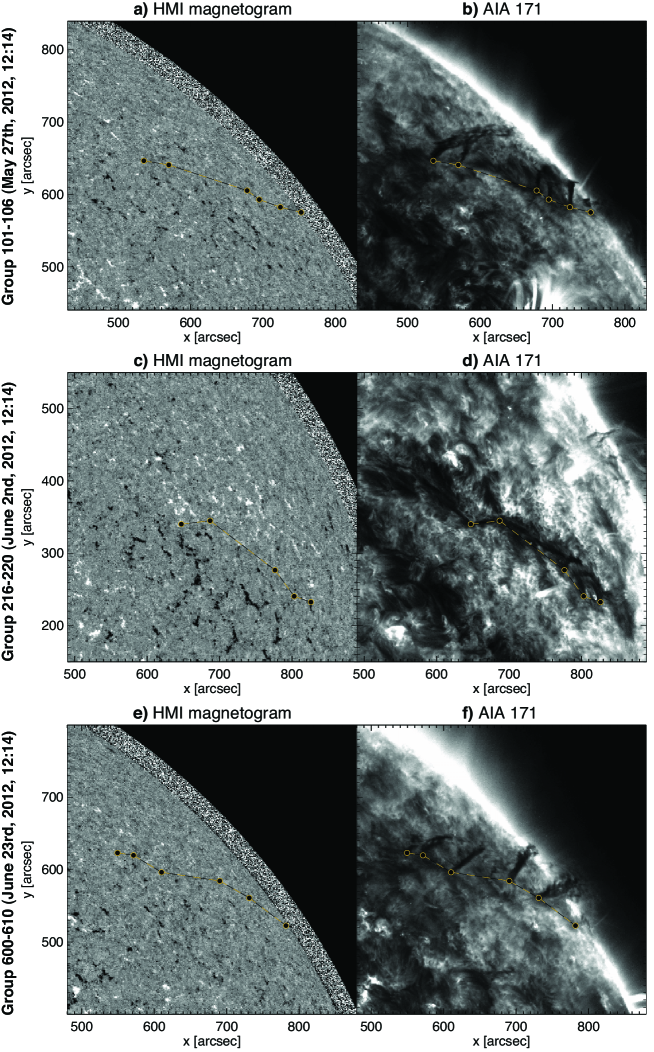
Figure 9.— HMI magnetograms (left column) and corresponding AIA 171 images (right column) for three selected tornado groups. The footpoints of the AIA 171 tornadoes, which are marked with circles and connected by lines in all panels, outline the polarity inversion lines in the magnetograms.

3.5. Tornado sizes in 171 Å images

The spatial extent of the tornadoes in the 171 Å images is measured for all confidently detected events for at least one or several snapshots, representing different stages in their evolution. The resulting data set consists of 392 tornado shapes. For each example, the footpoint and the centerline of the tornado followed along the structure are determined. Most tornadoes have centerline lengths between 10″ and 100″ ($\sim 7$ Mm - $75$ Mm). It is not always obvious where a tornado starts and where it ends. Adding the topmost part of the observed structure to the tornado instead of the prominence can lead to an overestimation of the lengths of the longest centerlines. The continuation into the prominence is better seen in 304 Å images (see Sect. 3.2). The width of the tornado is then measured along the centerline and usually increases from the footpoint outwards. With these uncertainties in mind, we determine the average tornado length to be $36.3\arcsec~{}\pm~{}19.0$″ (26.3 Mm $\pm 13.8$ Mm).

We derive a characteristic width for each example by averaging the width along the middle part of the centerline. The characteristic widths extend over a large range between mostly 2″and 16″ (1.5 Mm - 11.6 Mm) with a few smaller and larger cases (see Fig. 8a). On average the width is (6.1 $\pm$ 3.3) ″ (4.4 Mm $\pm$ 2.4 Mm).

In general, the width increases with the length, which implies that tornadoes scale to different sizes (see linear regression in Fig. 8d). About 80 % of all shapes have an aspect ratio, i.e. centerline length divided by characteristic width, of 8 or less (Fig. 8e-f). Many examples appear to have a rather straight centerline, whereas others are significantly curved. We define the curvedness of a tornado as the ratio of the path length of the spine and the distance between the footpoint and the most distant point. The resulting histogram is shown in Fig. 8g. In almost all cases the curvedness stays below 1.3. There is also a trend of larger curvedness with increasing tornado length.

The appearance of the tornadoes in the AIA 171 Å images is affected by the spatial resolution of the instrument and the formation of the intensity in the passband. The tornadoes certainly have a fine-structure on smaller spatial scales, which is more clearly visible with other diagnostics. For instance, our off-limb H$\alpha$ observations in Fig. 4 reveal thin threads with widths of $\leq{}0.5$″. Already Lin et al. (2005a) and Antolin & Rouppe van der Voort (2012) reported on SST observations of thread-like structures with widths of $\leq 0.3$″.

3.6. Connection to photospheric magnetic fields.

A polarity inversion line (PIL, also referred to as ‘neutral line’) separates regions on the Sun in which either one polarity dominates and is often co-located with a filament channel (cf. Zirker et al. 1998). We analysed the HMI magnetograms (see Fig. 9) and found that tornado groups are typically arranged along PILs in connection with a filament. About one third of the tornadoes in our sample (see Sect. 3.3) are so close to the limb that a PIL cannot reliably be determined. However, there are some clear cases for which the PIL extends notably on the disk. We find that at least 86 % of all identified tornadoes are located close to a PIL. It cannot be ruled out that the remaining cases are close to a (less obvious) PIL that was not clearly detected here.

It is hard to connect the footpoints of 171 Å AIA tornadoes to counterparts in the HMI magnetogram. We find no pronounced magnetic field concentrations close to where the footpoints are expected but, given the limited spatial resolution of HMI, only rather small-scale magnetic field concentrations. This is in line with the finding by Lin et al. (2005a) who show that the threads of quiescent filaments, whose footpoints we identify as tornadoes (see Sect. 4), are rooted in weak magnetic fields (see also Mackay et al. 2010, and references therein). According to Lin et al. (2005b), the majority ($\sim 2/3$) of the footpoints is located within the boundaries of the magnetic network in the photosphere, while the rest is connecting to weak fields in internetwork regions (cf. Płocieniak & Rompolt 1973).

Furthermore, we find groups of small magnetic flux concentrations with alternating polarity along the PIL. A possible explanation is that individual filament threads are rooted along the PIL and connect the different polarities over intermediate distances so that the loop tops compose an effectively longer filament spine. This hypothesis has to be tested through high-resolution magnetic field measurements of the kind demonstrated by Orozco Suárez et al. (2013) for a quiescent hedgerow prominence.

3.7. Eruption events

There are (at least) 36 tornadoes in our sample (18 %) that clearly end with an eruption. These tornadoes are organized in groups that form the legs of filament spines although the filament is not always clearly visible, e.g. when a group only appears at the limb shortly before eruption. Some prominences may only become visible shortly before their eruption (Engvold et al. 2001). Eruptions are best seen for the examples at the limb so that the number detected here is most likely a lower limit only.

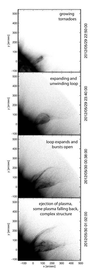
Figure 10.— Eruption of the tornado group that is shown in the upper row of Fig. 1. The uppermost panel shows the group shortly before eruption, whereas the other three panels show different stages of the eruption from top to bottom. The panels show inverted AIA 171 Å images, which have been enhanced for better visibility of the ejected plasma. The coordinates are centered on the footpoint of the initial tornado group.

As already noted by Su et al. (2012), tornadoes erupt together with the filament, which is expected if they are indeed part of the filament. The group shown in Fig. 10 consists of 5 tornadoes which appear close together at the west limb. The connecting filament spine is visible in time sequences together with plasma that appears to spiral upwards through the tornadoes into the filament spine. The tornadoes at the limb seem to grow in height prior to eruption, resulting in an extended absorption feature in the AIA 171 Å image (see uppermost panel in Fig. 10).

The eruption of the example in Fig. 10 begins with a pronounced loop, which most likely connects two of the former tornadoes. The lower parts of the loop appear to intersect, which may explain the observation that the loop unwinds and expands afterwards. The loop top seems to rise with an apparent speed that increases from 10 km/s to 30 km/s until it reaches a height of $\sim 200$ Mm beyond the limb. Then, the loop bursts open and plasma threads are ejected outwards with high speeds on the order of 200 km/s. We also observe material falling back down afterwards. Shortly after the eruption of this loop more loops appear, which are rooted at slightly different locations on the surface. We interpret it such that individual parts of the filaments, which connect different tornadoes in individual loops, erupt one after another. The eruption of the first loop possibly triggers the eruption of the other loops.

The initial growth of a tornado together with the rise of the filament and the cavity has also been observed by Su et al. (2012). A possible explanation is that the rotation of the magnetic field, which is most likely seen as a tornado, produces an increasing twist of the filament, which eventually becomes unstable and erupts (cf., e.g., Su & van Ballegooijen 2013; Yan et al. 2013). Eruptions due to the injection of helicity are also discussed in detail by, e.g., Zhang & Low (2005) and Zhang et al. (2006). The existence of resulting helical structures during prominence eruptions has been reported repeatedly (e.g., Su et al. 2012, and references therein).

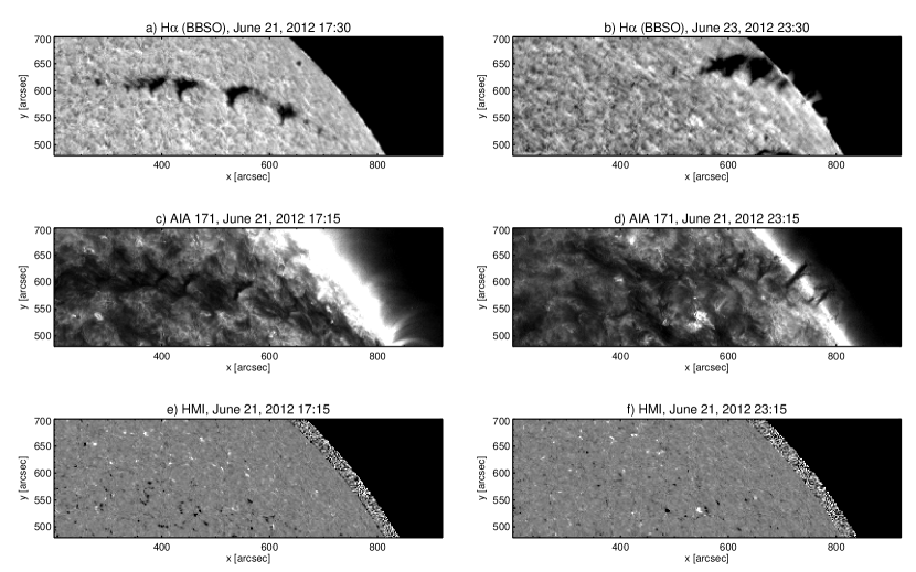
Figure 11.— The relation of tornadoes to filament channels and barbs illustrated for an exemplary tornado group at two different times (left column and right column). All panels show the same region on the Sun and display the BBSO H$\alpha$ images (top), the AIA 171 Å images (middle), and the corresponding HMI magnetograms (bottom).

4. Discussion

Tornadoes, filaments and barbs.

The conclusion that giant tornadoes are parts of filaments is supported by the fact that the vast majority of the tornadoes in our sample and possibly all of them are located along filament channels as seen in H$\alpha$ images and along polarity inversion lines (see Sect. 3.6), which are indicators of filaments in the atmosphere above (see Fig. 11). Already the spatial distribution of the tornadoes gives a hint of their nature. They are distributed mostly in the mid-latitudes, probably close to sunspot latitude belts, or at their boundaries, and in elongated groups. The fact that there are only few tornadoes observed close to the poles (see Fig. 2) also indicates that they are not entirely a quiet Sun phenomena, so rather intermediary. The more complex structure of active regions makes it more difficult to discern tornadoes there, which introduces a potential detection bias concerning events related to active region prominences. Most of the filaments with tornadoes reported here are therefore characterized as quiescent.

The example in Fig. 4 illustrates how different the same event appears in different diagnostics. The AIA 171 Å images show tornadoes as narrow elongated dark features. The spatial resolution of the observation certainly affects the determined length of the features since the parts towards the narrow footpoint of a tornado might not be resolved. Further differences are caused by the different formation of the intensity captured by different diagnostics so that effectively different parts of a tornado are mapped. We argue here that H$\alpha$ line core images mostly show the lower parts of tornadoes. Li et al. (2012) and Su et al. (2012) identify their tornadoes with ‘barbs’. They describe barbs as the observational signatures of tornadoes when seen from the side (cf. middle row in Fig. 10 by Martin 1998). For many events in our data set, we indeed find funnel-like dark features in H$\alpha$ at the exact same locations as the tornadoes (see the example in Fig. 11). We would like to remark that these funnel-like features may appear differently compared to what is referred to as ’barbs’ by other authors (see, e.g., Mackay et al. 1999; Joshi et al. 2013, and references therein). The example in Fig. 11 represents a situation, where the filament spine is barely visible in H$\alpha$, instead only a row of funnel-like features is seen. However, for other filaments with clearly visible spine it is obvious that giant tornadoes connect smoothly to the filament spine (see Fig. 4f) and that they seem to be composed of thin threads that extend from the chromosphere (see Fig. 4c). These characteristics are also found for barbs. Furthermore, we note that the barbs studied in detail by Li & Zhang (2013) in AIA 171 Å and H$\alpha$ images look identical to the tornadoes discussed here. For the 58 barbs in their sample, they derive an average length of 23.7 Mm, an average width of 2.1 Mm, and an average lifetime of 17.2 h. While the average length of barbs agrees well with the one for the 201 giant tornadoes derived here, barbs appear to be somewhat thinner and short-lived compared to the giant tornadoes, although this might be due to differences in the measurement details and/or the different sizes of the samples in the two studies. In conclusion, our results suggest that giant tornadoes are connected to funnel-like dark features close to filaments/prominences in H$\alpha$ images, which supports the view by Su et al. (2012). However, it has still to be shown if these features are equivalent to barbs or if this only holds under certain conditions and/or for certain stages during the evolution of filaments. For instance, tornadoes might simply be a sub-group of rotating barbs. A comprehensive definition of the terms ‘barb’ and ‘giant tornado’ might be key for solving this apparent controversy. Whether ‘barb’ or ‘tornado’ is the more suitable name is directly linked to the question if these events are truly rotating or not.

As seen in section 3.2, most of the SDO channels show tornadoes as dark absorption-like structures, indicating that it corresponds to plasma with temperatures outside the (coronal) ranges where the contribution functions of the channels are sensitive. Only the 304 Å AIA channel shows the tornado plasma in emission, and this indicates that part of it is at a temperature close to $8\times 10^{4}~{}$K. The off-limb tornado observed with the SST indicates a very cool temperature component with an average upper-limit temperature of 7 000 K. The threaded structure observed with the SST cannot be resolved with AIA, which prevents us from drawing conclusions about the thermal structure of tornadoes in general. The observed co-located emission in 304 Å AIA and H$\alpha$ images could be the result of a ’prominence corona transition region’ (Parenti & Vial 2007) or of a threaded sub-substructure with a mixture of cool and hot plasma. It is clear, however, that the very low temperatures agree with temperature diagnostics in prominences (Hirayama 1985), which therefore strongly supports our view that giant tornadoes constitute sources and sinks to prominences. The existence of such flows can be expected if barbs and tornadoes would indeed be connected as suggested by Su et al. (2012). The existence of upflows and/or downflows co-spatial to vortex motions has been reported repeatedly for magnetic structures of different sizes in the solar atmosphere (e.g., Bruzek 1974; Brueckner 1980; Brandt et al. 1988; Bonet et al. 2008; Wedemeyer-Böhm & Rouppe van der Voort 2009; Jess et al. 2009; Kamio et al. 2010; Zhang & Liu 2011). A final verification of this hypothesis requires further high-resolution observations of tornadoes and prominences.

In this respect, the finding that barbs are often already observed before the filament spine becomes visible (e.g. Pevtsov & Neidig 2005; Li et al. 2012; Su et al. 2012) could be interpreted such that they serve as initial plasma sources for prominences. We also find a group of tornadoes co-located with the forming prominence analysed by Berger et al. (2012), although it is not clear if these tornadoes play a role in the formation process. Furthermore, the Doppler shifts that we determined in Sect. 3.2 are of the same order as the speeds in counter-streaming flows in barbs as derived by Zirker et al. (1998).

The Interface Region Imaging Spectrograph (IRIS), which was launched in June 2013, is a promising instrument for detecting the lower to upper chromospheric parts of tornadoes and might shed light on many of the still open questions. IRIS is specially designed for spectrometric observations of the solar atmosphere in UV lines with high spatial and temporal resolutions. For instance, observations in the Mg II h $\&$ k lines ($\log\mathrm{T}=4.0~{}\mathrm{K}$) will have a cadence of $1-2~{}$s, a spatial resolution of $0.4\arcsec$ (with a field of view of $0.3\arcsec\times 40\arcsec$), an effective area of $0.25~{}\mathrm{cm}^{2}$ and a wavelength resolution of 80 mÅ.

The role of tornadoes in prominence eruptions.

Prominence eruptions are usually analyzed numerically and analytically in a scenario in which prominences are composed by a helical flux rope anchored in the photosphere (Kippenhahn & Schlüter 1957; Low & Hundhausen 1995). The magnetic twist found in this structure is usually attributed to gradual changes in the photospheric boundaries, compromising its stability by the increase of coronal magnetic stress. The latter can be achieved with sub-photospheric torsional Alfvén waves bringing twist to the coronal field or through reconnection between sheared magnetic loops from converging flows at the PIL, and occurs in a timescale of a few days (Démoulin & Aulanier 2010; Kusano et al. 2012). In this classical view, the prominence is generally seen as one whole structure. In the present work we have seen that a tornado can be considered as a magnetic entity having one end fixed at the photosphere and the other end connected to a large mass reservoir such as a prominence. In this view, tornadoes can not only be considered as legs to prominences but also as mass regulatory systems for the latter. Furthermore, the presented observations suggest a scenario in which tornadoes play an important role on the stability of the prominence. Along this view, it is important to consider whether conditions leading to a prominence eruption, like the injection of helicity (cf., e.g., Zhang & Low 2005; Zhang et al. 2006), may crucially depend on tornadoes.

The presence of rotation in tornadoes reported in this work and in Su et al. (2012) provides an image of a tornado reminiscent of that of the prominence flux rope with the main difference being that its axis is vertical instead of horizontal. As a first approximation we can therefore consider a tornado as a vertical flux rope with a fixed lower end (on the photosphere) and a somewhat looser upper end with higher degree of freedom rooted to a large mass reservoir. Along this view a tornado can become unstable and erupt from the loss of equilibrium and ideal MHD instability (Forbes & Priest 1995; Kliem & Török 2006; Démoulin & Aulanier 2010). A possible scenario in which such loss of equilibrium could happen is that set by the kink instability. If the winding of magnetic field lines along the tornado exceeds a threshold, the structure is deformed into a helical structure because of the current driven instability known as the kink instability (Priest 1982; Matsumoto et al. 1998). Hood & Priest (1979) and Linton et al. (1996) analyze the critical twist angle above which a flux tube is unstable against a kink mode. Values between $2\,\times\,\pi$ and $10\,\times\,\pi$ are found, depending on the magnetic field topology (uniformly twisted force-free field or other). For the case of the off-limb tornado observed by the SST, Doppler shifts around 20 km s^-1 are found, implying an angular velocity of 0.004 radians per second for the observed radius of $\sim 5$ Mm. In a low-beta plasma environment these speeds would imply a very fast magnetic field winding of one revolution every half an hour. It is therefore likely that a kink instability may be triggered. Along this view, we predict that the amount of twist found in a tornado is inversely proportional to its lifetime.

Rotating magnetic fields on different spatial scales.

Solar tornadoes are essentially spatially confined rotating magnetic field structures that seem to exist on a large range of spatial scales. The giant tornadoes discussed here tend to be larger than the magnetic tornadoes presented by Wedemeyer-Böhm et al. (2012), which have widths between 2″ and 5.5″, although 57 % of all cases have effective widths in that range, too (see Fig. 8). The off-limb tornado discussed in Sect. 3.2 has with a width of 6″ - 8″ at its base and is thus only slightly larger than the so far largest observed chromospheric swirl with a width of 5.5″. These two phenomena might therefore be related if not even just different sizes of the same scalable phenomenon. We investigate this hypothesis by plotting the abundance and the lifetimes of giant and magnetic tornadoes over their characteristic size (see Fig. 12). The characteristic size is here defined as the typical diameter perpendicular to the rotation axis in the upper atmosphere. Based on the diameters derived in this study (see Sect. 3.5 and Fig. 8c), giant tornadoes are larger and persist longer but appear in smaller numbers than magnetic tornadoes. It should be noted that magnetic tornadoes have only been detected near disk-center as chromospheric swirls so far, while the AIA 171 Å imprint of giant tornadoes is difficult to see there, resulting in much reduced number of detections in the central region of the disk (see Fig. 2).

Li et al. (2012) report on an extremely large tornado with a complicated fine-structure, which seems to be much larger than the examples discussed here. Li et al. determine a radius of 35 Mm for the circular trajectory of a plasma blob, which they track in the AIA 171 Å images, and specify a duration of 3 hours for the clearest revolution. By revisiting these data, we find that the tornado described by Li et al. can be followed for almost half a day and that it is co-located with a long-lived group of tornadoes, which are of the same type as those presented here (e.g., in Fig. 1). Among the giant tornadoes in the group, there is a pair, which is located not far from the apparent footpoint of the large-scale helical structure. This tornado pair seems to already exist at least 38 hours (or possibly days) before the helical event but it is no longer visible once the large-scale tornado develops. The connection between the giant tornadoes of the type described here and the large-scale helical event reported by Li et al. is not clear yet. The latter seems to be connected to the photosphere by several threads whereas such a fine-structure may not be resolved for the giant tornadoes. We mark the corresponding characteristic size of 70 Mm with a thick vertical line in Fig. 12 because the abundance of this type of tornado is unclear yet. It might be as high as the abundance of the giant tornadoes presented in this work or possibly less.

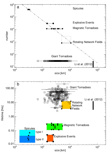
Figure 12.— Comparison of different rotating magnetic phenomena on the Sun: Giant tornadoes (squares), Rotating Network Fields (diamonds), magnetic tornadoes (triangles, tip downward), Explosive Events (circles), and spicules (triangles, tip upwards). a) Estimated total numbers of events as a function of their characteristic spatial scale. b) Lifetimes versus characteristic size. Measurements of the same giant tornado at different times are connected by solid lines. The individual data points are explained in the text in Sect. 4. The dot-dashed line in the upper panel represents a double-logarithmic power law for all phenomena except for the giant tornadoes.

Tornadoes are not the only observed examples of rotating magnetic structures. Phenomena that combine rotation and magnetic fields are known to span a large range of spatial scales in the atmosphere of the Sun. Among them are, e.g., so-called ‘Explosive Events’ (EEs) or swirling transition region jets (Curdt et al. 2012; Curdt & Tian 2011; Dere et al. 1989; Innes 2004), EUV cyclones or ‘Rotating Network Magnetic Fields’ (RNFs, Zhang & Liu 2011) and macrospicules (Pike & Harrison 1997; Banerjee et al. 2000; Scullion et al. 2009; Murawski et al. 2011). More examples may or may not include the rotation and/or helicity in coronal jets (Patsourakos et al. 2008; Nisticò et al. 2009; Liu et al. 2011; Shen et al. 2011), motions in spicules (Suematsu et al. 2008; De Pontieu et al. 2012; Sekse et al. 2013), macroscopic EUV jets (Sterling et al. 2010), ‘spinning magnetic twist jet(s)’ (Shibata 1997) and rotating sunspots (Vemareddy et al. 2012). In the following, we compare these phenomena to solar tornadoes.

For rotating magnetic network fields (or EUV cyclones), we adopt the average lifetime of 3.5 hours given by Zhang & Liu (2011), although they present two examples with lifetimes of 12 and 9 hours, respectively. The characteristic width is estimated to be in the range between 7″ and 15″. Zhang & Liu state that 5600 RNFs are present every day across the whole Sun. Based on the average lifetime of 3.5 hours, we conclude that about 830 RNFs would be present on the Sun at all times. This number would increase to 2800 for a lifetime of 12 hours (see dotted line for RNFs in Fig. 12a).

Explosive Events (EEs, also known as Swirling Transition Region Jets) are observed spectroscopically in radiation that originates from the transition region. Curdt et al. (2012) characterize EEs as bi-directional flows, which last typically for one to three minutes, have spatial extents of 1500 km to 2500 km and exhibit Doppler velocities of $\pm(50-150)\,\mathrm{km\,s}^{-1}$. According to Teriaca et al. (2004), 30 000 EEs exist at all times.

Spicules would be placed at the small end of spatial scales but it is not clear yet if the torsional motions reported by De Pontieu et al. (2012) qualify spicules as rotating magnetic structures or if the detected motions are related to Alfvén waves that propagate on a non-rotating magnetic field structure. For spicules, we adopt the mean values for lifetimes and widths from Pereira et al. (2012, see their Tables 3 and 4). Spicules are the most abundant and shortest-lived events considered here.

At first glance, the total number $N_{i}$ of most of the different phenomena seems to be correlated to their characteristic size $\bar{x}_{i}$. The correlation can be approximated with the double-logarithmic power law

$$N_{i}=7.1\,\times\,10^{9}+\bar{x}_{i}^{\ \ -1.7}\qquad,$$ (2)

which fits for the considered phenomena with exception of the giant tornadoes (see dot-dashed line in Fig. 12). For some so far unknown reason, giant tornadoes seem not numerous enough and too narrow to fit the trend that is found for the other phenomena. Possible reasons might be connected to the finding that giant tornadoes are the legs of prominences, whereas the other phenomena are individual events that are not directly connected to large-scale structures.

Implications for other stars.

Tornadoes can be expected to exist also in the atmospheres of cooler stars because basic ingredients for a tornado, namely photospheric vortex flows and magnetic fields, are most likely common there, too. Photospheric vortex flows have been found in a numerical simulation of a M-type dwarf star by Ludwig et al. (2006). More recently, Wedemeyer et al. (2013) report on a first example of a (small-scale) magnetic tornado in a numerical radiation magnetohydrodynamics simulation that includes magnetic fields and a chromosphere for a M-type dwarf star. It remains to be seen if also giant tornadoes can form in the atmospheres of cool stars.

5. Conclusions

Our findings support the suggestion by Su et al. (2012) that giant tornadoes are connected to filaments. We find many examples of tornado groups, which first appear as coherent filaments on disk and only become visible as individual tornadoes when the structure rotates closer towards the solar limb (less than $\sim 160$″). The tornadoes appear to connect smoothly to the filament spine in the atmosphere above, which has been observed for barbs before (e.g Zirker et al. 1998). Both the SDO and SST observations presented here suggest the existence of a cool plasma flow along the tornado axis with temperatures typical to the lower to upper chromosphere, although this finding has to be confirmed in a future more detailed study. This result strongly supports our view that tornadoes can act as sources and sinks for prominences. The SST observations also suggest that tornadoes rotate around their vertical axis. The numerical model of small-scale solar tornadoes by Wedemeyer-Böhm et al. (2012), in which tornadoes are driven by photospheric vortex flows, exhibits flows that spiral both upwards and downwards with speeds comparable to the values found for filament barbs. In agreement with Su et al. (2012), we conclude that this rotation could lead to an increasing twist of the magnetic structure of the overlying prominence until it becomes unstable and erupts. We observed several examples of tornado groups, which are unambiguously connected to erupting prominences. It seems therefore likely that the rotation of tornadoes could be a common trigger of prominence eruptions, although this conclusion has to be investigated further. Erupting prominences cause Coronal Mass Ejections (CMEs) which often eject large amounts of coronal plasma into the interplanetary space (Bothmer & Schwenn 1994). Monitoring of giant tornadoes might therefore provide a way to forecast CMEs, in case their role as trigger of eruptions is confirmed by future studies.

References

- Antolin & Rouppe van der Voort (2012) Antolin, P. & Rouppe van der Voort, L. 2012, ApJ, 745, 152
- Anzer & Heinzel (2005) Anzer, U. & Heinzel, P. 2005, ApJ, 622, 714
- Banerjee et al. (2000) Banerjee, D., O’Shea, E., & Doyle, J. G. 2000, A&A, 355, 1152
- Berger et al. (2012) Berger, T. E., Liu, W., & Low, B. C. 2012, ApJ, 758, L37
- Bonet et al. (2008) Bonet, J. A., Márquez, I., Sánchez Almeida, J., Cabello, I., & Domingo, V. 2008, ApJ, 687, L131
- Bothmer & Schwenn (1994) Bothmer, V. & Schwenn, R. 1994, Space Sci. Rev., 70, 215
- Brandt et al. (1988) Brandt, P. N., Scharmer, G. B., Ferguson, S., Shine, R. A., & Tarbell, T. D. 1988, Nature, 335, 238
- Brueckner (1980) Brueckner, G. E. 1980, Highlights of Astronomy, 5, 557
- Bruzek (1974) Bruzek, A. 1974, in IAU Symposium, Vol. 57, Coronal Disturbances, ed. G. A. Newkirk, 323
- Bruzek & Durrant (1977) Bruzek, A. & Durrant, C. J., eds. 1977, Astrophysics and Space Science Library, Vol. 69, Illustrated glossary for solar and solar-terrestrial physics
- Curdt & Tian (2011) Curdt, W. & Tian, H. 2011, A&A, 532, L9+
- Curdt et al. (2012) Curdt, W., Tian, H., & Kamio, S. 2012, Sol. Phys., 280, 417
- De Pontieu et al. (2012) De Pontieu, B., Carlsson, M., Rouppe van der Voort, L. H. M., et al. 2012, ApJ, 752, L12
- Démoulin & Aulanier (2010) Démoulin, P. & Aulanier, G. 2010, ApJ, 718, 1388
- Dere et al. (1989) Dere, K. P., Bartoe, J.-D. F., Brueckner, G. E., & Recely, F. 1989, ApJ, 345, L95
- Domingo et al. (1995) Domingo, V., Fleck, B., & Poland, A. I. 1995, Sol. Phys., 162, 1
- Engvold (1998) Engvold, O. 1998, in Astronomical Society of the Pacific Conference Series, Vol. 150, IAU Colloq. 167: New Perspectives on Solar Prominences, ed. D. F. Webb, B. Schmieder, & D. M. Rust, 23
- Engvold et al. (2001) Engvold, O., Jakobsson, H., Tandberg-Hanssen, E., Gurman, J. B., & Moses, D. 2001, Sol. Phys., 202, 293
- Forbes & Priest (1995) Forbes, T. G. & Priest, E. R. 1995, ApJ, 446, 377
- Harrison et al. (1995) Harrison, R. A., Sawyer, E. C., Carter, M. K., et al. 1995, Sol. Phys., 162, 233
- Hill et al. (2004) Hill, F., Bogart, R. S., Davey, A., et al. 2004, in Society of Photo-Optical Instrumentation Engineers (SPIE) Conference Series, Vol. 5493, Society of Photo-Optical Instrumentation Engineers (SPIE) Conference Series, ed. P. J. Quinn & A. Bridger, 163–169
- Hirayama (1985) Hirayama, T. 1985, Sol. Phys., 100, 415
- Hood & Priest (1979) Hood, A. W. & Priest, E. R. 1979, Sol. Phys., 64, 303
- Innes (2004) Innes, D. E. 2004, in ESA Special Publication, Vol. 547, SOHO 13 Waves, Oscillations and Small-Scale Transients Events in the Solar Atmosphere: Joint View from SOHO and TRACE, ed. H. Lacoste, 215
- Jess et al. (2009) Jess, D. B., Mathioudakis, M., Erdélyi, R., et al. 2009, Science, 323, 1582
- Joshi et al. (2013) Joshi, A. D., Srivastava, N., Mathew, S. K., & Martin, S. F. 2013, Sol. Phys.
- Kamio et al. (2010) Kamio, S., Curdt, W., Teriaca, L., Inhester, B., & Solanki, S. K. 2010, A&A, 510, L1
- Kippenhahn & Schlüter (1957) Kippenhahn, R. & Schlüter, A. 1957, ZAp, 43, 36
- Kliem & Török (2006) Kliem, B. & Török, T. 2006, Physical Review Letters, 96, 255002
- Kusano et al. (2012) Kusano, K., Bamba, Y., Yamamoto, T. T., et al. 2012, ApJ, 760, 31
- Lemen et al. (2012) Lemen, J. R., Title, A. M., Akin, D. J., et al. 2012, Sol. Phys., 275, 17
- Li & Zhang (2013) Li, L. & Zhang, J. 2013, Sol. Phys., 282, 147
- Li et al. (2012) Li, X., Morgan, H., Leonard, D., & Jeska, L. 2012, ApJ, 752, L22
- Lin et al. (2005a) Lin, Y., Engvold, O., Rouppe van der Voort, L., Wiik, J. E., & Berger, T. E. 2005a, Sol. Phys., 226, 239
- Lin et al. (2005b) Lin, Y., Wiik, J. E., Engvold, O., Rouppe van der Voort, L., & Frank, Z. A. 2005b, Sol. Phys., 227, 283
- Linton et al. (1996) Linton, M. G., Longcope, D. W., & Fisher, G. H. 1996, ApJ, 469, 954
- Liu et al. (2011) Liu, C., Deng, N., Liu, R., et al. 2011, ApJ, 735, L18
- Low & Hundhausen (1995) Low, B. C. & Hundhausen, J. R. 1995, ApJ, 443, 818
- Ludwig et al. (2006) Ludwig, H.-G., Allard, F., & Hauschildt, P. H. 2006, A&A, 459, 599
- Mackay et al. (2010) Mackay, D. H., Karpen, J. T., Ballester, J. L., Schmieder, B., & Aulanier, G. 2010, Space Sci. Rev., 151, 333
- Mackay et al. (1999) Mackay, D. H., Longbottom, A. W., & Priest, E. R. 1999, Sol. Phys., 185, 87
- Martin (1998) Martin, S. F. 1998, Sol. Phys., 182, 107
- Matsumoto et al. (1998) Matsumoto, R., Tajima, T., Chou, W., Okubo, A., & Shibata, K. 1998, ApJ, 493, L43
- Murawski et al. (2011) Murawski, K., Srivastava, A. K., & Zaqarashvili, T. V. 2011, A&A, 535, A58
- Nisticò et al. (2009) Nisticò, G., Bothmer, V., Patsourakos, S., & Zimbardo, G. 2009, Sol. Phys., 259, 87
- Orozco Suárez et al. (2012) Orozco Suárez, D., Asensio Ramos, A., & Trujillo Bueno, J. 2012, ApJ, 761, L25
- Orozco Suárez et al. (2013) Orozco Suárez, D., Asensio Ramos, A., & Trujillo Bueno, J. 2013, in Highlights of Spanish Astrophysics VII, 786–791
- Panasenco et al. (2013) Panasenco, O., Martin, S. F., & Velli, M. 2013, ArXiv e-prints
- Panesar et al. (2013) Panesar, N. K., Innes, D. E., Tiwari, S. K., & Low, B. C. 2013, A&A, 549, A105
- Parenti & Vial (2007) Parenti, S. & Vial, J.-C. 2007, A&A, 469, 1109
- Patsourakos et al. (2008) Patsourakos, S., Pariat, E., Vourlidas, A., Antiochos, S. K., & Wuelser, J. P. 2008, ApJ, 680, L73
- Pereira et al. (2012) Pereira, T. M. D., De Pontieu, B., & Carlsson, M. 2012, ApJ, 759, 18
- Pettit (1932) Pettit, E. 1932, ApJ, 76, 9
- Pettit (1950) Pettit, E. 1950, PASP, 62, 144
- Pevtsov & Neidig (2005) Pevtsov, A. A. & Neidig, D. 2005, in Astronomical Society of the Pacific Conference Series, Vol. 346, Large-scale Structures and their Role in Solar Activity, ed. K. Sankarasubramanian, M. Penn, & A. Pevtsov, 219
- Pike & Harrison (1997) Pike, C. D. & Harrison, R. A. 1997, Sol. Phys., 175, 457
- Pike & Mason (1998) Pike, C. D. & Mason, H. E. 1998, Sol. Phys., 182, 333
- Płocieniak & Rompolt (1973) Płocieniak, S. & Rompolt, B. 1973, Sol. Phys., 29, 399
- Priest (1982) Priest, E. R. 1982, Solar magneto-hydrodynamics, 74P
- Scharmer et al. (2003a) Scharmer, G. B., Bjelksjo, K., Korhonen, T. K., Lindberg, B., & Petterson, B. 2003a, in Society of Photo-Optical Instrumentation Engineers (SPIE) Conference Series, ed. S. L. Keil & S. V. Avakyan, Vol. 4853, 341
- Scharmer et al. (2003b) Scharmer, G. B., Dettori, P. M., Lofdahl, M. G., & Shand, M. 2003b, in Society of Photo-Optical Instrumentation Engineers (SPIE) Conference Series, Vol. 4853, Society of Photo-Optical Instrumentation Engineers (SPIE) Conference Series, ed. S. L. Keil & S. V. Avakyan, 370–380
- Scharmer et al. (2008) Scharmer, G. B., Narayan, G., Hillberg, T., et al. 2008, ApJ, 689, L69
- Scherrer et al. (2012) Scherrer, P. H., Schou, J., Bush, R. I., et al. 2012, Sol. Phys., 275, 207
- Scullion et al. (2009) Scullion, E., Popescu, M. D., Banerjee, D., Doyle, J. G., & Erdélyi, R. 2009, ApJ, 704, 1385
- Sekse et al. (2012) Sekse, D. H., Rouppe van der Voort, L., & De Pontieu, B. 2012, ApJ, 752, 108
- Sekse et al. (2013) Sekse, D. H., Rouppe van der Voort, L., De Pontieu, B., & Scullion, E. 2013, ApJ, 769, 44
- Shen et al. (2011) Shen, Y., Liu, Y., Su, J., & Ibrahim, A. 2011, ApJ, 735, L43
- Shibata (1997) Shibata, K. 1997, in ESA Special Publication, Vol. 404, Fifth SOHO Workshop: The Corona and Solar Wind Near Minimum Activity, ed. A. Wilson, 103
- Sterling et al. (2010) Sterling, A. C., Harra, L. K., & Moore, R. L. 2010, ApJ, 722, 1644
- Su & van Ballegooijen (2013) Su, Y. & van Ballegooijen, A. 2013, ApJ, 764, 91
- Su et al. (2012) Su, Y., Wang, T., Veronig, A., Temmer, M., & Gan, W. 2012, ApJ, 756, L41
- Suematsu et al. (2008) Suematsu, Y., Ichimoto, K., Katsukawa, Y., et al. 2008, in Astronomical Society of the Pacific Conference Series, Vol. 397, First Results From Hinode, ed. S. A. Matthews, J. M. Davis, & L. K. Harra, 27
- Teriaca et al. (2004) Teriaca, L., Banerjee, D., Falchi, A., Doyle, J. G., & Madjarska, M. S. 2004, A&A, 427, 1065
- van Noort et al. (2005) van Noort, M., Rouppe van der Voort, L., & Löfdahl, M. G. 2005, Sol. Phys., 228, 191
- Vemareddy et al. (2012) Vemareddy, P., Ambastha, A., & Maurya, R. A. 2012, ApJ, 761, 60
- Vissers & Rouppe van der Voort (2012) Vissers, G. & Rouppe van der Voort, L. 2012, ApJ, 750, 22
- Wedemeyer et al. (2013) Wedemeyer, S., Ludwig, H.-G., & Steiner, O. 2013, Astronomische Nachrichten, 334, 137
- Wedemeyer-Böhm & Rouppe van der Voort (2009) Wedemeyer-Böhm, S. & Rouppe van der Voort, L. 2009, A&A, 507, L9
- Wedemeyer-Böhm et al. (2012) Wedemeyer-Böhm, S., Scullion, E., Steiner, O., et al. 2012, Nature, 486, 505
- Yan et al. (2013) Yan, X. L., Pan, G. M., Liu, J. H., et al. 2013, AJ, 145, 153
- Zhang & Liu (2011) Zhang, J. & Liu, Y. 2011, ApJ, 741, L7+
- Zhang et al. (2006) Zhang, M., Flyer, N., & Low, B. C. 2006, ApJ, 644, 575
- Zhang & Low (2005) Zhang, M. & Low, B. C. 2005, ARA&A, 43, 103
- Zirker (1989) Zirker, J. B. 1989, Sol. Phys., 119, 341
- Zirker et al. (1998) Zirker, J. B., Engvold, O., & Martin, S. F. 1998, Nature, 396, 440
- Zöllner (1869) Zöllner, F. 1869, Astronomische Nachrichten, 74, 269