Bethe ansatz description of edge-localization in the open-boundary XXZ spin chain

Abstract

At large values of the anisotropy $\Delta$, the open-boundary Heisenberg spin-$\frac{1}{2}$ chain has eigenstates displaying localization at the edges. We present a Bethe ansatz description of this ‘edge-locking’ phenomenon in the entire $\Delta>1$ region. We focus on the simplest spin sectors, namely the highly polarized sectors with only one or two overturned spins, i.e., one-particle and two-particle sectors.

Edge-locking is associated with pure imaginary solutions of the Bethe equations, which are not commonly encountered in periodic chains. In the one-particle case, at large $\Delta$ there are two eigenstates with imaginary Bethe momenta, related to localization at the two edges. For any finite chain size, one of the two solutions become real as $\Delta$ is lowered below a certain value.

For two particles, a richer scenario is observed, with eigenstates having the possibility of both particles locked on the same or different edge, one locked and the other free, and both free either as single magnons or as bound composites corresponding to ‘string’ solutions. For finite chains, some of the edge-locked spins get delocalized at certain values of $\Delta$ (‘exceptional points’), corresponding to imaginary solutions becoming real. We characterize these phenomena thoroughly by providing analytic expansions of the Bethe momenta for large chains, large anisotropy $\Delta$, and near the exceptional points. In the large-chain limit all the exceptional points coalesce at the isotropic point ($\Delta=1$) and edge-locking becomes stable in the whole $\Delta>1$ region.

1 Introduction

General context.

The effects on many-body systems exerted by localized features such as edges and impurities have long been a central theme of condensed matter physics. Kondo physics [1] and Anderson orthogonality catastrophe [2] are among the most celebrated examples of complex physics caused by single impurities. An edge of a finite system can also be responsible for families of effects. Among other phenomena, an edge can bind or lock excitations or particles. Intriguingly, in addition to single-particle binding at boundaries and edges, edge-locking can also arise as a collective interaction-induced phenomenon, which results in unintuitive temporal dynamics [3, 4].

Edges appear naturally through the use of open boundary conditions. Periodic boundary conditions are, of course, far more popular due to the presence of translation symmetry and due to having physical momentum as a good quantum number. In particular, in the Bethe ansatz approach to one-dimensional (1D) systems, the bulk of the literature focuses on periodic chains. Nevertheless, since the discovery of the exact solution of the spin-$\frac{1}{2}$ Heisenberg chain with boundary magnetic fields [5, 6], integrable models have provided a rich playground to investigate edge-related physics in 1D. Example topics studied are edge bound states in integrable field theories [7, 8, 9, 10, 11, 12], Kondo-like behaviors in spin chains [13, 14, 15, 16, 17], Friedel oscillations [18], Anderson orthogonality catastrophe [19, 20, 21], with also potential applications in quantum computing devices [22, 23].

In this work, we focus on the anisotropic Heisenberg (XXZ) chain, and examine structures that appear in the spectra due to the presence of open boundary conditions (edges), in particular those eigenstates whose spatial forms are dictated by the edge. In these eigenstates, one or more “particles” (overturned spins) are localized or locked at the edges. In the sectors we look at (one or two particles), most of these features are physically simple and show up as prominent band structures in the spectrum, as we show below in Figure 1. However, a Bethe ansatz description has been lacking in the literature to the best of our knowledge, despite the relevant Bethe equations having been available since the work of Refs. [5, 6].

The open-boundary Heisenberg XXZ chain.

The open-boundary anisotropic spin-$1\over 2$ Heisenberg XXZ chain of $L$ interacting spins is described by the Hamiltonian

$${\mathcal{H}}=\frac{1}{2}\sum_{i=1}^{L-1}(S_{i}^{+}S_{i+1}^{-}+S_{i}^{-}S_{i+1}^{+})+\Delta\sum_{i=1}^{L-1}S_{i}^{z}S_{i+1}^{z}$$ (1)

Here $S_{i}^{+,-,z}$ are given as $S_{i}^{\pm}\equiv(\sigma_{i}^{x}\pm i\sigma_{i}^{y})/2,S_{i}^{z}\equiv\sigma_{i}^{z}/2$, with $\sigma_{i}^{x,y,z}$ the Pauli matrices, and $\Delta$ is the anisotropy. The sites $i=1$ and $i=L$ are endpoints and are only coupled to one neighbor each. The Hilbert space of (1) is spanned by $2^{L}$ basis states, which are conveniently generated starting from the fully polarized eigenstate $\left|0\right.\rangle\equiv\left|\uparrow\uparrow\uparrow\cdots\uparrow\right.\rangle$ with all the spins up, and overturning $M$ of the spins, with $M\in[0,L]$. As conventional in the Bethe ansatz literature, we refer to overturned spins as “particles”.

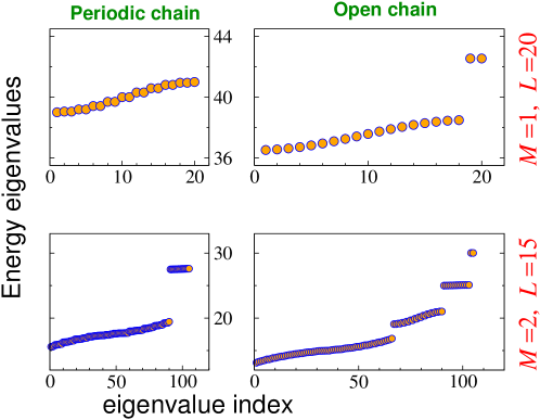
Figure 1: Comparison of the energy spectra of periodic and open chains, $M=1$ and $M=2$ sectors, obtained by numerical diagonalization of the Hamiltonian at $\Delta=10$. Energy eigenvalues are ordered in increasing algebraic order.

We restrict to the highly polarized sectors of (1) with only one ($M=1$) and two ($M=2$) particles. The spectral effect of open boundary conditions in these sectors is shown in Figure 1, where periodic and open boundary conditions are compared through numerical diagonalization. The extra structures in the open-chain cases clearly represent edge physics: for example, the top two eigenstates correspond to the one ($M=1$) or two ($M=2$) particles localized at the two edges of the chain.

In this work, through explicit consideration of the full spectrum of (1) via the Bethe ansatz formalism, we provide a complete classification of edge-locking behavior in the whole region $1<\Delta<\infty$ in the $M=1,2$ sectors.

Outline of main results.

We show that edge-locking is clearly reflected in the nature of the solutions of the Bethe equations (Bethe momenta): while locked particles correspond to pure imaginary momenta, extended or magnon-like behavior is signaled by real solutions.

As a consequence, edge-locking provides a useful physical criterion for classifying the Bethe momenta. In fact, a byproduct of our analysis is a complete scrutiny of the full set of solutions of Bethe equations in the $M=1,2$ sectors at $1<\Delta<\infty$. This is similar to what has been done in [24, 25] for the isotropic ($\Delta=1$) Heisenberg model with periodic boundary conditions.

In the $M=1$ sector, there is a single Bethe momentum describing the eigenstates and only two types of eigenstates are possible. The Bethe momentum is either real, corresponding to a spatially extended particle, or purely imaginary, corresponding to the particle being edge-locked. Due to reflection symmetry, the eigenstates with edge-locking are linear combinations of configurations with locking at the left edge and at the right edge. There are clearly two such eigenstates at large $\Delta$. Remarkably, for any finite chain length $L$, as $\Delta$ is lowered there is a value of $\Delta$ where one of these eigenstates gets delocalized, and the corresponding Bethe momentum becomes real instead of imaginary. Motivated by real$\leftrightarrow$imaginary transformation effects in the literature on non-hermitian matrices, we refer to such special $\Delta$ values as “exceptional points”.

In the $M=2$ sector a richer scenario arises: eigenstates can have both particles edge-locked (fully edge-locked states), or no edge-locking (both particles spatially extended or magnon-like), or have one particle edge-localized and the other spatially extended. These classes correspond to different classes of Bethe momenta: both momenta imaginary, both real or a complex conjugate pair, one real and one imaginary. At large $\Delta$, using geometric arguments, one can find the numbers of different classes of eigenstates, as simple functions of $L$ (Section 4). At smaller $\Delta$, there are several series of exceptional points at which imaginary momenta become real, and eigenstates lose part or all of their edge-locked nature, i.e, particles “delocalize”.

In both $M=1,2$ sectors, two fully edge-locked eigenstates form a doublet of quasi-degenerate energy levels, which is separated from the rest of the spectrum by a gap $\sim\Delta$, as can be seen in Figure 1. The energy splitting within the doublet vanishes exponentially with the system size. In the $M=2$ case, these are eigenstates where the two particles are localized on the same edge. A third fully edge-locked state has one particle localized at each edge; this state is not spectrally separated but has an intriguingly simple structure (Section 6.3).

In this work we throughly characterize the natures of the eigenstates in the Bethe ansatz language, by providing the numbers of different classes of eigenstates at different $\Delta$ values, the locations of the exceptional points $\Delta_{e}$, analytic expressions for the Bethe momenta at large $\Delta$ and large $L$ and in the vicinity of the exceptional points, etc. The values of the exceptional points are described by a set of two coupled equations that we provide explicitly. An intriguing feature is that in the limit $L\to\infty$ all the exceptional points coalesce at the isotropic point $\Delta=1$, signaling that edge-locked particles become stable in the whole region $1<\Delta<\infty$. Finally, we discuss $M=2$ eigenstates where the particles are extended but mutually bound, which correspond to complex conjugate pairs of Bethe momenta, and are closely analogous to “2-strings” well-known from the periodic chain. These eigenstates are found to be stable in the whole $\Delta>1$ region, i.e. no unbinding of bound states or locking at the boundary is observed.

Organization of this Article.

In section 2 we outline the Bethe ansatz formulation for the open XXZ chain, following [5]. Section 3 describes the one-particle ($M=1$) sector, characterizing edge-locked and extended states and the exceptional point below which one of the edge-locked states becomes extended. The next six sections, 4 to 9, detail the two-particle ($M=2$) sector. We start this discussion in Section 4 with an outline of the different types of solutions expected at large $\Delta$ from physical expectations of edge-locking, and then describe the different types of solutions (real+real, imaginary+imaginary, real+imaginary, complex conjugate pairs) in the next few sections, respectively Sections 5, 6, 7, 8. We end the discussion of the $M=2$ sector in Section 9 with an overview of the spectrum, more detailed than that provided in Figure 1. Section 10 concludes the article.

2 Bethe ansatz approach

We start with setting up the notation for the Bethe ansatz approach [5, 6, 26, 27] for the XXZ spin chain with open boundary conditions. First, since the total magnetization $S_{T}^{z}\equiv\sum_{i}S^{z}_{i}=L/2-M$, $M$ being the number of particles, is a conserved quantity, it can be used to label the eigenstates of (1). We denote as $|\Psi_{M}\rangle$ an eigenstate of (1) in the sector with $M$ particles. This, for any $\Delta$, can be written in general as

$$|\Psi_{M}\rangle=\sum\limits_{1\leq j_{1}<j_{2}<\dots<j_{M}\leq L}A_{M}(j_{1},j_{2},j_{3}...,j_{M})|j_{1},j_{2},j_{3}....j_{M}\rangle$$ (2)

where the sum is over the positions $1\leq j_{n}\leq L$ ($n=1,2,\dots,M$) of the particles in the chain, while $A_{M}(\{j_{n}\})$ is the amplitude of the eigenstate component with particles at positions $j_{1},j_{2},\dots,j_{M}$. In the Bethe ansatz approach one rewrites (2) as

$$A_{M}(j_{1},j_{2},\dots,j_{M})\leavevmode\nobreak\ =\leavevmode\nobreak\ \sum\limits_{\bar{\mathcal{P}}}(-1)^{\epsilon_{\bar{\mathcal{P}}}}\,B_{M}(k_{\bar{\mathcal{P}}_{1}},k_{\bar{\mathcal{P}}_{2}},\dots,k_{\bar{\mathcal{P}}_{M}})\,e^{i(k_{\bar{\mathcal{P}}_{1}}j_{1}+k_{\bar{\mathcal{P}}_{2}}j_{2}+\dots+k_{\bar{\mathcal{P}}_{M}}j_{M})}$$ (3)

Here the sum is over all the permutations and (arbitrary number of) reflections $k_{i}\to-k_{i}$ of the so-called Bethe momenta $k_{1},k_{2},\dots,k_{M}$, while $\epsilon_{\bar{\mathcal{P}}}$ is given as $\epsilon_{\bar{\mathcal{P}}}\equiv\epsilon_{\mathcal{P}}+\varepsilon$, with $\epsilon_{\mathcal{P}}$ the sign of the permutation $\mathcal{P}$ and $\varepsilon$ the number of reversed momenta. The Bethe momenta $k_{\ell}$ with $\ell=1,2,\dots,M$ are solutions of the non linear set of equations (Bethe equations)

$$e^{2i(L+1)k_{\ell}}=\frac{(1-\Delta e^{ik_{\ell}})^{2}}{(1-\Delta e^{-ik_{\ell}})^{2}}\prod_{j=1,j\neq\ell}^{M}\frac{(1+e^{i(k_{j}-k_{\ell})}-2\Delta e^{ik_{j}})(1+e^{i(k_{\ell}+k_{j})}-2\Delta e^{ik_{\ell}})}{(1+e^{i(k_{\ell}+k_{j})}-2\Delta e^{ik_{j}})(1+e^{i(k_{j}-k_{\ell})}-2\Delta e^{-ik_{\ell}})}$$ (4)

In terms of $\{k_{\ell}\}$ the amplitude $B_{M}$ is given as

$$B_{M}\leavevmode\nobreak\ =\leavevmode\nobreak\ \prod\limits_{j=1}^{M}(1-\Delta e^{ik_{j}})e^{-i(L+1)k_{j}}\prod\limits_{1\leq j<\ell\leq M}(1+e^{i(k_{\ell}-k_{j})}-2\Delta e^{ik_{\ell}})(1+e^{i(k_{j}+k_{\ell})}-2\Delta e^{ik_{j}})e^{-ik_{\ell}}$$ (5)

For each set of solutions of (4) one has that (2) is an eigenstate of (1). The corresponding energy is given as

$$E=\sum\limits_{i=1}^{M}\cos k_{i}+E_{0}(L,M),\qquad E_{0}(L,M)\equiv\Big{(}\frac{L-1}{4}-M\Big{)}\Delta$$ (6)

Note that the amplitude $A_{M}(\{k_{\ell}\})$ is identically zero for $k_{\ell}=0$ and $k_{\ell}=\pi$, implying that these Bethe momenta, although formally solutions of the Eqs. (4), are not allowed.

The amplitude (3) is symmetric under permutations and reflections of the momenta $k_{1},k_{2},\dots,k_{M}$. This symmetry is inherited by the Bethe momenta $\{k_{\ell}\}$, i.e. given the set of solution of (4) as ${\mathcal{K}}\equiv\{k_{\ell}\}$, any other set obtained by permuting and inverting an arbitrary number of elements of ${\mathcal{K}}$ is also a set of solutions of (4). Thus one can restrict to the positive solutions of (4), i.e. requiring $k_{\ell}>0\,\,\forall\,\ell$. This also implies that only half of the complex plane is allowed for $k_{\ell}$. Here we choose the right half, i.e., we impose $\textrm{Re}(k)>0$. Note that, for purely imaginary momenta ($\textrm{Re}(k)=0$) only half of the imaginary axis is allowed (we impose $\textrm{Im}(k)>0$). Finally, using the invariance $k_{\ell}\to-k_{\ell}$ and the $2\pi$ periodicity of the functions appearing in (4) one can also restrict to $\textrm{Re}(k)<\pi$. The resulting region of allowed values for the Bethe momenta in the complex plane is shown in Figure 2.

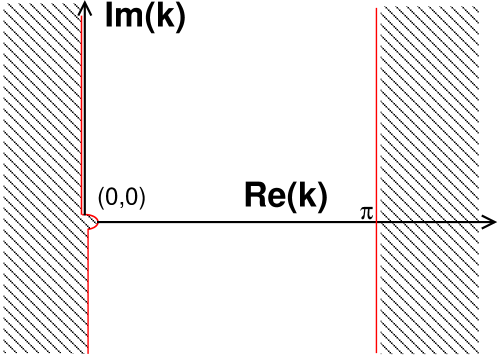
Figure 2: Allowed values for the Bethe momenta $k\equiv(\textrm{Re}(k),\textrm{Im}(k))$ in the complex plane, for the open-boundary XXZ chain. The dashed area represents the excluded regions The line $\textrm{Re}(k)=\pi$ is excluded. Purely imaginary momenta with $\textrm{Im}(k)>0$ are allowed.

Comparison with periodic case.

For periodic boundary conditions, the Bethe equations would be given as

$$e^{iLk_{\ell}}=\prod_{j=1,j\neq\ell}^{M}\left[-\frac{1+e^{i(k_{\ell}+k_{j})}-2\Delta^{ik_{\ell}}}{1+e^{i(k_{\ell}+k_{j})}-2\Delta e^{ik_{j}}}\right]\,.$$ (7)

In the periodic case the Bethe momenta are not restricted to a half-plane and can range in the interval $\textrm{Re}(k)\in(-\pi,\pi]$, i.e., double the region shown in Figure 2.

For the same $M$ sector, the Bethe equations are more complicated in the open-boundary case [compare Eq. (4) with Eq. (7)]; so it is not surprising that the open-boundary case has more structure such as the possibility of purely imaginary solutions.

3 The one particle sector: extended versus edge-locked behavior

In this section we will treat the one-particle sector ($M=1$).

The total number of eigenstates, i.e., solutions to the Bethe equations (4), is equal to the chain length $L$. Since the energy eigenvalues must be real, Eq. (6) constrains the solutions of (4) to be either purely real or purely imaginary. Real solutions correspond to spin wave states (magnons), which are extended in the bulk of the chain, whereas purely imaginary Bethe momenta correspond to edge-locked ones. These are eigenstates with the particle exponentially localized at the edges of the chain.

The number of imaginary solutions (edge-locked eigenstates) depends on the anisotropy $\Delta$ and on chain length $L$. The situation is summarized in Figure 3. At large $\Delta$ there are two imaginary momenta ($k_{\pm}$). For each fixed size $L$ we find that there exists an “exceptional” value of the anisotropy, $\Delta=\Delta_{e}$, at which one of the purely imaginary solutions passes through zero and becomes purely real. For $\Delta\leq\Delta_{e}$ the Bethe equations admit only one imaginary solution. Clearly, the number of real solutions is $L-2$ and $L-1$ for respectively $\Delta>\Delta_{e}$ and $\Delta<\Delta_{e}$ respectively.

The imaginary solution surviving in the region $\Delta<\Delta_{e}$ itself vanishes at $\Delta\to 1$. This means that $\Delta=1$ is also an exceptional point, and that pure imaginary momenta are not present at $\Delta=1$. We show below, and have found numerically, that $\Delta_{e}=(L+1)/(L-1)$, so that $\Delta_{e}$ decreases monotonically upon increasing the chain size and coalesces to $\Delta_{e}\to 1$ in the limit $L\to\infty$.

3.1 The magnon states

We first consider the extended eigenstates, i.e., real solutions of the Bethe equations. The corresponding Bethe momenta are obtained by solving the equation

$$e^{2ik(L+1)}=\frac{(1-\Delta e^{ik})^{2}}{(1-\Delta e^{-ik})^{2}}$$ (8)

As usual in the Bethe ansatz literature, we consider the Bethe equation in logarithmic form. First we redefine the momentum $k$ in terms of the so-called rapidity $\lambda$:

$$k=\pi-2\arctan\frac{\tan\lambda}{\tanh(\eta/2)}-2\pi\left\lfloor\frac{\lambda}{\pi}+\frac{1}{2}\right\rfloor$$ (9)

where $\eta$ is related to the anisotropy $\Delta$ as $\eta\equiv\textrm{arcosh}(\Delta)$. The term with the floor function $\lfloor\cdot\rfloor$ is convenient in order to make $k$ continuous as function of $\lambda$ in the interval $[0,\pi]$. Taking the logarithm on both sides in (8) one obtains

$$\arctan\frac{\tan\lambda}{\tanh(\eta/2)}+\pi\left\lfloor\frac{\lambda}{\pi}+\frac{1}{2}\right\rfloor=\frac{\pi J}{2(L+1)}+\frac{1}{L+1}\left[\arctan\left(\frac{\tan 2\lambda}{\tanh\eta}\right)+\left\lfloor\frac{2\lambda}{\pi}+\frac{1}{2}\right\rfloor\right]$$ (10)

Here the integer $J$ ($J\in[1,L]$) is the so-called Bethe quantum number. Each choice of $J$ identifies, in principle, an eigenstate of (1). The corresponding energy expressed in terms of $\lambda$ reads

$$E=-\cos\Big{(}2\arctan\frac{\tan\lambda}{\tanh(\eta/2)}+2\pi\left\lfloor\frac{\lambda}{\pi}+\frac{1}{2}\right\rfloor\Big{)}+E_{0}(L,1)$$ (11)

Figure 3(a) shows real solutions obtained from the Bethe equation. For $\Delta>\Delta_{e}$, real rapidities and hence real momenta are found by using values $J=1,2,\dots,L-2$. For $\Delta<\Delta_{e}$, there is an extra real solution as $J=L-1$ also gives a real rapidity. In the Figure, the special value is $\Delta_{e}=$ 2(1.4) for $L=$ 3(6), consistent with the relation $\Delta_{e}=(L+1)/(L-1)$ derived below.

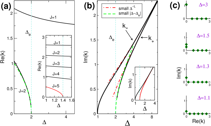
Figure 3: Solutions of the Bethe equation in the $M=1$ sector as a function of $\Delta$. In (a,b), main panels show $L=3$ and insets show $L=6$. (a) Real solutions. The Bethe number $J$ is noted for each solution. There are $L-1$ real solutions for $\Delta<\Delta_{e}=\frac{L+1}{L-1}$ and $L-2$ real solutions for $\Delta>\Delta_{e}$. One real solution ($J=L-1$) vanishes as $\Delta\to\Delta_{e}^{-}$. The dashed dotted line is the analytic expression in the vicinity of $\Delta_{e}$. (b) Imaginary solutions. Logarithmic scale on the horizontal axis. There are two imaginary momenta at $\Delta>\Delta_{e}$; one of them ($k_{+}$) vanishes at $\Delta=\Delta_{e}$. The dashed and dashed-dotted lines are the analytic expansions respectively at $\Delta\to\Delta_{e}$ and at large $\Delta$. (c) Solutions on complex-momentum plane, $L=6$, shown for a sequence of $\Delta$ values above and below $\Delta_{e}=1.4$. Real and imaginary axes have different scales.

3.2 The edge-locked states (half-strings)

In this section we discuss the nature of the imaginary solutions of the Bethe equations and their evolution as function of $\Delta$ across the exceptional point $\Delta_{e}$. Due to the restriction $\textrm{Im}(k)>0$, the purely imaginary strings do not appear in complex conjugate pairs. For this reason we refer to them as “half-strings”.

Figure 3(b) plots the two imaginary solutions ($k_{+},k_{-}$) of the Bethe equations (12) for an open XXZ chain with $L=3$ as function of $\Delta$. At $\Delta>\Delta_{e}$, two imaginary momenta are present. At $\Delta\to\Delta_{e}$ one of the two ($k_{+}$) vanishes. This solution re-emerges on the other side of $\Delta_{e}$ as a real solution. This can be seen on the sequence of plots in Figure 3(c).

In order to study the imaginary solutions of (8) we start redefining $i\log z\equiv k$ with $z$ real. Since $\textrm{Im}(k)>0$ (Figure 2), we have $z>1$. The Bethe equation is

$$z^{-2L}=\frac{(z-\Delta)^{2}}{(1-\Delta z)^{2}}$$ (12)

Clearly the left side in Eq. (12) vanishes exponentially upon increasing $L$. To recover the same behavior in the right side one has to impose $z=\Delta+{\mathcal{O}}(e^{-L})$. Substituting this ansatz into (12) one finds two solutions $z_{\pm}$ as

$$z_{\pm}=\Delta\pm\left[\frac{1}{\Delta^{L-2}}-\frac{1}{\Delta^{L}}\right]\leavevmode\nobreak\ +\leavevmode\nobreak\ \mathcal{O}(\Delta^{-L-1})$$ (13)

The two solutions are nearly degenerate with the splitting decreasing exponentially with $L$. The argument above, i.e. matching of the behaviors of the two sides of (12) in the large $L$ limit, is similar to the argument used originally by Bethe to argue the presence of string solutions [7, 26].

The analytic result for $k_{\pm}$, Eq. (13), compares well with the exact numerical solution of (12) at large $\Delta$, as seen in Figure 3(b). The large-$\Delta$ result (13) does not include the vanishing behavior of $k_{+}$ at $\Delta_{e}$, but for $k_{-}$ it works reasonably down to $\Delta$ values lower than $\Delta_{e}$.

3.3 The exceptional point $\Delta_{e}$

In the vicinity of $\Delta_{e}$, we numerically observe $\textrm{Im}(k_{+})\sim c_{+}(\Delta-\Delta_{e})^{1/2}$. Plugging this ansatz into Eq. (12), Taylor expanding both sides in $(\Delta-\Delta_{e})$, and collecting the coefficient of $(\Delta-\Delta_{e})^{1/2}$, one obtains

$$\Delta_{e}\leavevmode\nobreak\ =\leavevmode\nobreak\ \frac{L+1}{L-1}$$ (14)

Considering the next non-zero order in $(\Delta-\Delta_{e})$, we further obtain

$$c_{+}=\sqrt{\frac{6(L-1)}{L(L+1)}}$$ (15)

It turns out that the vanishing real momentum in Fig. 3 (a) is described by the same function $\sim c_{+}(\Delta_{e}-\Delta)^{1/2}$. Comparison between the analytic expansions obtained above and the numerical solutions of the Bethe equations are shown in Fig. 3 (a) and (b). From (14), we note that $\Delta_{e}\to 1$ at $L\to\infty$, signaling that edge-locking persists in both eigenstates in the complete region $\Delta\in(1,\infty)$.

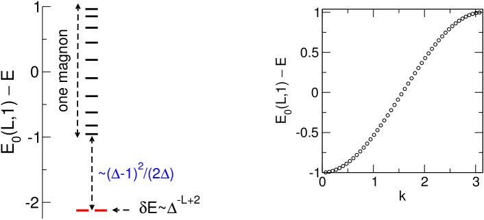
Figure 4: Energy spectrum of the open XXZ chain in the $M=1$ sector at $\Delta=4$, obtained from numerical solution of the Bethe equations. Left: $L=12$. We invert the energies and add $E_{0}(L,1)\equiv(L-5)\Delta/4$ so that the magnon (delocalized) part of the spectrum appears in the $(-1,1)$ range, and the edge-locked doublet appears at the bottom. The doublet is separated from the magnon states by a gap that scales as $\sim(\Delta-1)^{2}/(2\Delta)$ at large $\Delta$. Right panel: $E_{0}(L,1)-E$ versus the Bethe momentum $k$ for the magnon states (levels above the gap in the left figure). Data for a chain with $L=48$ at $\Delta=4$.

3.4 Signature of edge-locking in the energy spectrum

We now discuss the spectrum of the open-boundary XXZ chain in the one particle sector. In Figure 4 we show $E_{0}(L,1)-E$ at $\Delta=4$; here $E_{0}(L,1)\equiv\frac{1}{4}(L-5)\Delta$. Note that $4>\Delta_{e}=13/11$.

The half-strings $k_{\pm}$ correspond to a doublet of quasi degenerate energies at the bottom of the inverted spectrum and are separated by a gap from higher levels. Energy levels above the gap correspond to real solutions of the Bethe equations and exhibit the one-magnon dispersion (11) (similar to periodic boundary conditions). This is shown in more detail in the inset for a chain with $L=48$ plotting $E_{0}(L,1)-E$ versus the Bethe momentum $k$.

The gap scales as $\sim\frac{1}{2}\Delta$ for large $\Delta$ and does not depend on the system size, as expected for a surface localized state. More precisely the energy of the edge-locked doublet (using (11) and (13)) is given as $E_{0}(L,1)-E\sim-(1+\Delta^{2})/(2\Delta)$, implying that the distance from the bottom of the one magnon band (obtained at $k\sim 0$) is $\sim(\Delta-1)^{2}/(2\Delta)$. The splitting between the two levels forming the doublet decreases exponentially with the system size (as $\Delta^{-L+2}$).

3.5 Edge-locked eigenfunctions

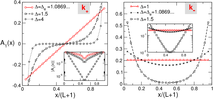
Figure 5: Spatial structure of edge-locked one-particle eigenstates. Wavefunction amplitude $A_{1}(x)$, obtained from the Bethe equations for chain length $L=24$, are plotted against $x/(L+1)$, $x$ being the particle position. Left and right panels correspond respectively to the imaginary solutions $k_{+}$ and $k_{-}$. Insets demonstrate exponential localization by plotting same data as in main figures on log-linear scale. Left ($k_{+}$) panel: continuous red line is the result at the exceptional point $\Delta_{e}=\frac{L+1}{L-1}$, where this imaginary solution becomes real. Right ($k_{-}$) panel: continuous red line is the wavefunction at the isotropic point $\Delta=1$, where this imaginary solution becomes real.

We now highlight the edge-locked nature of the doublet at the bottom of the inverted energy spectrum in Figure 4 by analyzing the corresponding eigenfunctions.

These are shown in Figure 5, plotting wavefunction components $A_{1}(x)$ against $x/(L+1)$, with $x\in[1,L]$ being the position of the particle in the chain. We consider the eigenfunctions obtained from the two imaginary solutions $k_{+}$, $k_{-}$.

Both eigenfunctions exhibit exponential localization at the edges of the chain at $\Delta>\Delta_{e}=25/23\sim 1.0869$. Their form in the large $\Delta$ limit is $\psi(k_{\pm})=(|1\rangle\mp|L\rangle)/\sqrt{2}$, $|1\rangle,|L\rangle$ being the configurations with the particle localized at the first and last site of the chain. The superposition is a consequence of the left-right symmetry of the chain, i.e., symmetry under inversion, ${\mathcal{I}}:i\to L-i+1$.

The eigenfunction obtained from $k_{-}$ is localized for any $\Delta>1$, and it becomes “flat” in the limit $\Delta\to 1$. The eigenfunction corresponding to $k_{+}$ becomes “linear” at $\Delta\to\Delta_{e}$. This observation provides an alternative way of determining the value of the exceptional point $\Delta_{e}$. Let us consider the “linear” superposition

$$|\psi\rangle=\alpha\sum\limits_{x=1}^{L}c_{x}|x\rangle,\qquad c_{x}\equiv x-(L+1)/2,\qquad\alpha\equiv(\sum_{x=1}^{L}|c_{x}|^{2})^{-1/2}$$ (16)

with $|x\rangle$ denoting the configuration with particle at position $x$. Now one can require that (16) is an exact eigenstate of the XXZ hamiltonian (1) with eigenvalue (from Figure 3 it is $k_{+}\to 0$ at $\Delta\to\Delta_{e}$)

$$E=1+E_{0}(L,1),\qquad E_{0}(L,1)\equiv(L-5)\Delta_{e}/4$$ (17)

Using the Schrödinger equation, one can write

$$E\equiv\langle\psi|H|\psi\rangle=|\alpha|^{2}(\sum_{x=2}^{L-1}c_{x}c_{x+1}+\Delta_{e}(c_{1}^{2}+c_{L}^{2})/2)+\Delta_{e}(L-5)/4$$ (18)

and equating (17) and (18) one obtains $\Delta_{e}$ as

$$\Delta_{e}=2\frac{\sum_{x=1}^{L}|c_{x}|^{2}-\sum_{x=2}^{L-1}c_{x}c_{x+1}}{(c_{1}^{2}+c_{L}^{2})}=(L+1)/(L-1)$$ (19)

which is the same result obtained in 3.3.

4 The two particle sector: overview

The rest of the Article, from this section up to Section 9, details the $M=2$ sector. In this section, we provide an overview, outlining the different types of two-particle eigenstates.

Bethe equations.

Each eigenstate in the two-particle sector is labeled by two Bethe momenta $k_{1}$ and $k_{2}$, whose possible values are given by two coupled equations:

$$e^{i2(L+1)k_{1}}\frac{(1-\Delta e^{-ik_{1}})^{2}}{(1-\Delta e^{ik_{1}})^{2}}=\frac{(1+e^{i(k_{1}+k_{2})}-2\Delta e^{ik_{1}})(1+e^{i(-k_{1}+k_{2})}-2\Delta e^{ik_{2}})}{(1+e^{i(k_{1}+k_{2})}-2\Delta e^{ik_{2}})(1+e^{i(-k_{1}+k_{2})}-2\Delta e^{-ik_{1}})}$$ (20)

$$e^{i2(L+1)k_{2}}\frac{(1-\Delta e^{-ik_{2}})^{2}}{(1-\Delta e^{ik_{2}})^{2}}=\frac{(1+e^{i(k_{1}+k_{2})}-2\Delta e^{ik_{2}})(1+e^{i(-k_{2}+k_{1})}-2\Delta e^{ik_{1}})}{(1+e^{i(k_{1}+k_{2})}-2\Delta e^{ik_{1}})(1+e^{i(-k_{2}+k_{1})}-2\Delta e^{-ik_{2}})}$$ (21)

The two equations are related by exchange of $k_{1}$ and $k_{2}$. The energy eigenvalue for the generic two-particle eigenstate reads

$$E=\cos(k_{1})+\cos(k_{2})+E_{0}(L,2),\qquad E_{0}(L,2)\equiv(L-9)\Delta/4$$ (22)

Types of solutions.

The condition that the energy (22) is real, allows four possibilities for the momentum pairs $(k_{1},k_{2})$:

$$\textrm{Im}\,(k_{1})=\textrm{Im}\,(k_{2})=0\qquad$$ both real

$$\textrm{Re}\,(k_{1})=\textrm{Re}\,(k_{2})=0\qquad$$ both imaginary

$$\textrm{Im}\,(k_{1})=\textrm{Re}\,(k_{2})=0\qquad$$ one real and one imaginary

$$k_{1}=k_{2}^{*}\qquad$$ complex conjugate pair (string)

Note that the trivial solutions $k_{1}=k_{2}=0$ and $k_{1}=k_{2}=\pi$ have to be discarded and one can restrict to the region of the complex plane depicted in Figure 2.

The physical meanings of the four different types of eigenstates are illustrated via real-space configurations shown in Table 1. At large $\Delta$, the edge-localization or mutual binding is strong. The eigenstates are then closely represented by the types of configurations shown in Table 1. Therefore, at large $\Delta$ we can use combinatorial arguments on the number of available configurations to count the number of eigenstates of different type. This is shown in the second column of Table 1.

Table 1: Classification of the $\frac{1}{2}L(L-1)$ two-particle eigenstates at large $\Delta$ and large $L$. Particle configurations (left column) and number of eigenstates (center column) for each type of solution of the Bethe equations (right column). Re (Im) stands for pure real (imaginary) momenta. Symbols $\fullmoon$ and $\newmoon$ denote bulk particles and boundary particles respectively. Symbols $\otimes$ denote sites where particles are not allowed. Subscripts denote fixed positions. First row: states that do not exhibit edge-locking. Second row: states with one edge-locked particle and one extended particle. Third row: fully edge-locked states.

configurations	Number of states	Momenta $\mathbf{\{k_{1},k_{2}\}}$
$|\otimes_{1}\cdots\fullmoon\cdots\otimes\cdots\fullmoon\cdots\otimes_{L}\rangle$	$(L-3)(L-4)/2$	{Re, Re}
$|\otimes_{1}\cdots\fullmoon\fullmoon\cdots\otimes_{L}\rangle$	$L-3$	String
$|\newmoon_{1}\otimes_{2}\cdots\fullmoon\cdots\otimes_{L}\rangle$
$\pm$	$2(L-3)$	{Re, Im}
$|\otimes_{1}\cdots\fullmoon\cdots\otimes_{L-1}\newmoon_{L}\rangle$
$|\newmoon_{1}\newmoon_{2}\cdots\rangle+|\cdots\newmoon_{L-1}\newmoon_{L}\rangle$	1
$|\newmoon_{1}\cdots\newmoon_{L}\rangle$	1	{Im, Im}
$|\newmoon_{1}\newmoon_{2}\cdots\rangle-|\cdots\newmoon_{L-1}\newmoon_{L}\rangle$	1

The {Re,Re} solutions correspond to eigenstates where the two particles are not locked at the edges and not bound to each other. The number of such solutions/eigenstates is therefore the number of ways of placing the two particles in non-adjacent, non-boundary, sites, hence $\frac{1}{2}(L-3)(L-4)$. The number of string (complex conjugate) solutions — eigenstates where the two particles are extended but mutually bound — is the number of ways of placing the two particles in neighboring non-boundary sites, hence $(L-3)$. The {Re,Im} solutions correspond to eigenstates where one particle is edge-locked and the other is extended. The number of such solutions is the number of ways one can place a particle at one edge and the other in a non-adjacent, non-edge position, hence $2(L-3)$. Finally, there are three fully edge-locked eigenstates given by {Im,Im} solutions — two with a bound pair at the same edge and one with the two particles at two edges. Of course, the eigenstates all have definite parity under reflection; we have therefore used linear combinations of left-edge-locked and right-edge-locked configurations where appropriate. For example, of the three fully edge-locked eigenstates, two are symmetric under ${\mathcal{I}}:i\to L-i+1$, and one is antisymmetric.

Smaller $\Delta$.

The scenario outlined in Table 1 is true for large $\Delta$. Since the localization length scale increases with decreasing $\Delta$, it is perhaps not very surprising that this picture gets modified at smaller anisotropies. For each fixed $L$ we find that the number of edge-locked particles changes as function of $\Delta$. While in the one particle sector ($M=1$) this corresponds to a transition from one pure imaginary to real momentum (“delocalization” of the edge-locked state), here a richer scenario appears with several types of delocalization transitions between the different classes of momentum pairs in Table 1.

For each fixed $L$ two of the three fully edge-locked states ($\{\textrm{Im}$, $\textrm{Im}\}$ type in Table 1) decay at two distinct exceptional points $\Delta_{e,1}^{(ii)}<\Delta_{e,2}^{(ii)}$. As $\Delta$ approaches the exceptional point one of the two imaginary momenta forming the pair vanishes and emerges on the other side (of the exceptional point) as a real momentum, i.e. the transformation $\{\textrm{Im},\textrm{Im}\}\to\{\textrm{Re},\textrm{Im}\}$ occurs. The resulting pair $\{\textrm{Re},\textrm{Im}\}$ survives at $\Delta>1$. Interestingly, the remaining edge-locked state disappears only in the limit $\Delta\to 1$.

Similar behavior is shown by the type $\{\textrm{Re},\textrm{Im}\}$. At fixed $L$ half of the states (i.e. $L-3$ states) become magnon-like upon lowering $\Delta$, i.e. one has the transformation $\{\textrm{Re},\textrm{Im}\}\to\{\textrm{Re},\textrm{Re}\}$. These transitions occur at $L-3$ (one for each state) exceptional points $\Delta^{(r,i)}_{e,\ell}$ with $\ell=1,2,\dots,L-3$. The remaining $L-3$ edge-locked states decay only in the limit $\Delta\to 1$. Finally, the string states are found to be stable in the whole range $1<\Delta<\infty$, i.e., there is no unbinding.

It is worth stressing that for periodic boundary conditions the structure of solutions of the Bethe equations outlined in Table 1 becomes strikingly simpler. In fact only the first row survives and one has, at least in the large $\Delta$ regime, $L$ complex conjugate momenta (strings) and $L(L-3)/2$ real momentum pairs.

5 Extended states of two non-bound particles: real momentum pairs

In this section we focus on the set of real solutions of Eqs. (20)(21), i.e. {Re,Re} in Table 1). To this purpose it is convenient to rewrite the Bethe equations in logarithmic form. Taking the logarithm on both sides of (20)(21) one obtains

$$(L+1)k_{1}= \pi J_{1}-2\arctan\frac{\Delta\sin k_{1}}{1-\Delta\cos k_{1}}-\arctan\frac{\Delta\sin(\frac{k_{1}+k_{2}}{2})}{\cos(\frac{k_{1}-k_{2}}{2})-\Delta\cos(\frac{k_{1}+k_{2}}{2})}$$ (23)

$$-\arctan\frac{\Delta\sin(\frac{k_{1}-k_{2}}{2})}{\cos(\frac{k_{1}+k_{2}}{2})-\Delta\cos(\frac{k_{1}-k_{2}}{2})}$$

$$(L+1)k_{2}= \pi J_{2}-2\arctan\frac{\Delta\sin k_{2}}{1-\Delta\cos k_{2}}-\arctan\frac{\Delta\sin(\frac{k_{2}+k_{1}}{2})}{\cos(\frac{k_{1}-k_{2}}{2})-\Delta\cos(\frac{k_{2}+k_{1}}{2})}$$ (24)

$$-\arctan\frac{\Delta\sin(\frac{k_{2}-k_{1}}{2})}{\cos(\frac{k_{1}+k_{2}}{2})-\Delta\cos(\frac{k_{2}-k_{1}}{2})}$$

In contrast to the one particle case, we do not redefine the Bethe momenta in terms of the rapidity variables $\lambda$. Here $J_{1}$ and $J_{2}$ are the Bethe quantum numbers ($J_{1},J_{2}\in[1,L]$). Since exchanging $J_{1}$ and $J_{2}$ has the effect of swapping $k_{1}\leftrightarrow k_{2}$, and since $J_{1}=J_{2}$ would imply $k_{1}=k_{2}$, one can restrict to $J_{1}<J_{2}$. The counting of the remaining possibilities gives $L(L-1)/2$ possible real solutions for (24). We anticipate that as for periodic boundary conditions, however, only some pairs $(J_{1},J_{2})$ of Bethe numbers give real solutions. Note also that for periodic boundary conditions one would have the condition $k_{1}+k_{2}=2\pi/L(J_{1}+J_{2})$ (conservation of total momentum), reducing the analog of equations (23)(24) to a single variable equation.

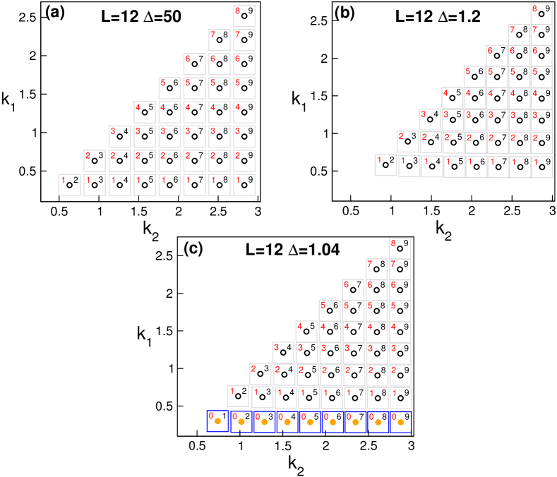
Figure 6: Real solutions ($k_{1}$,$k_{2}$) of the Bethe equations for the two-particle ($M=2$) sector; $L=12$ chain. The ($k_{1}$,$k_{2}$) values are shown as circles and the accompanying numbers inside boxes are the corresponding Bethe quantum numbers $(J_{1},J_{2})$. The same Bethe numbers appear with the real solutions at $\Delta=50$ and $\Delta=1.2$; panels (a) and (b). Panel (c) shows a $\Delta$ value below the region of exceptional points $\Delta_{e}^{(rr)}$. An extra row of real momentum pairs with Bethe numbers $J_{1}=0$, $J_{2}=1,2,\dots,L-3$ is now present.

We first observe that the first two terms in the r.h.s. of (23) (24) are not continuous as function of $k_{1},k_{2}$ in the interval of interest, $k_{1},k_{2}\in(0,\pi)$. This can be avoided by means of the following redefinitions

$$\arctan\frac{\Delta\sin k_{i}}{1-\Delta\cos k_{i}}\to\arctan\frac{\Delta\sin k_{i}}{1-\Delta\cos k_{i}}-\pi\theta(k_{i}-\arccos(1/\Delta))$$ (25)

$$\arctan\frac{\Delta\sin(\frac{k_{i}+k_{j}}{2})}{\cos(\frac{k_{i}-k_{j}}{2})-\Delta\cos(\frac{k_{i}+k_{j}}{2})}\to \arctan\frac{\Delta\sin(\frac{k_{i}+k_{j}}{2})}{\cos(\frac{k_{i}-k_{j}}{2})-\Delta\cos(\frac{k_{i}+k_{j}}{2})}-$$

$$\pi\theta\left(k_{j}-2\arccos\frac{(1+\Delta)\sin\frac{k_{i}}{2}}{\sqrt{1+\Delta^{2}-2\Delta\cos k_{i}}}\right)$$

Note the presence of the Heavside step functions $\theta(x)\equiv(1+\textrm{sign}(x))/2$ in (25)(5), which contribute with a $\pm\pi$ phase shift (depending on the interplay between the Bethe momenta and $\Delta$) in the Bethe equations. This amounts to a redefinition of the Bethe numbers $J_{1},J_{2}$, and it is simple to understand in the Ising limit $\Delta\to\infty$. One has then

$$\arctan\frac{\Delta\sin k_{i}}{1-\Delta\cos k_{i}}\to-k_{i}+\pi\theta(2k_{i}-\pi)$$ (27)

$$\arctan\frac{\Delta\sin(\frac{k_{i}+k_{j}}{2})}{\cos(\frac{k_{i}-k_{j}}{2})-\Delta\cos(\frac{k_{i}+k_{j}}{2})}\to-\frac{k_{i}+k_{j}}{2}+\pi\theta(k_{j}+k_{i}-\pi)$$ (28)

implying that, given a solution $k_{i}$ of the Bethe equations, the corresponding Bethe number $J_{i}$ is shifted by $1$ if $k_{i}>\pi/2$ (cf. (27)). Another additional shift is obtained if $k_{i}+k_{j}>\pi$ (cf. (28)).

The Bethe momenta $k_{1},k_{2}$, obtained from numerical solutions of (23), (24), with the redefinitions (25), (5), are shown in Figure 6 for a $L=12$ chain, for three $\Delta$ values. For each pair $(k_{1},k_{2})$ the corresponding Bethe quantum numbers $(J_{1},J_{2})$ are also reported.

At $\Delta=50$ the Bethe momenta appear to be “quantized” in units of $\pi/(L-2)$ forming a triangular structure in the plane $k_{2},k_{1}$. Moreover “bands” of quasi degenerate momenta $k_{1}$ and $k_{2}$ are present, respectively “rows” and “columns” of solutions in the Figure. Solutions within the same row (column) have the same quantum number $J_{1}$ ($J_{2}$). A similar structure persists at much lower values of $\Delta$ as seen for $\Delta=1.2$ in Figure 6(b). The same triangular structure is observed apart from deviations at small $k_{1}$, $k_{2}$.

The simple structure of the Bethe numbers observed in Figure 6 depends crucially on (25), (5). A striking consequence of using (25), (5) is that all the pairs of Bethe numbers $1\leq J_{1}<J_{2}\leq L-3$ correspond to real solutions of the Bethe equations. Also the set of Bethe numbers does not depend on the anisotropy $\Delta$ (the same integer pairs $(J_{1},J_{2})$ give the Bethe momenta of both Figure 6 (a) and (b)). With a different redefinition (different choice of branches of the $\arctan$ function), the set of $J_{1}$, $J_{2}$ values giving real solutions can be different.

Finally, Figure 6(c) plots the solutions of the Bethe equations at $\Delta=1.04$. Now, we find that $L-3$ extra real momentum pairs appear as a new row at the bottom of the triangle; these correspond to Bethe numbers $J_{1}=0$ and $J_{2}=1,2,\dots,L-3$. At large $\Delta$ these extra real solutions undergo the transformation $\{\textrm{Re},\textrm{Re}\}\to\{\textrm{Re},\textrm{Im}\}$ and disappear. This transformation is discussed in the next subsection.

5.1 {Re,Re}$\to${Re,Im} transformations: edge-locking of a single particle at exceptional points

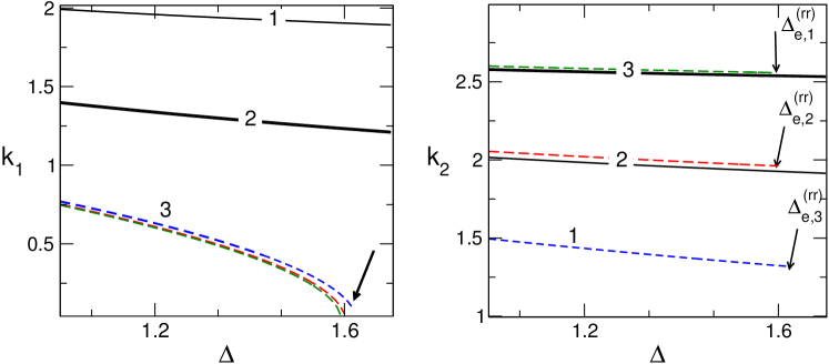
Figure 7: Real solutions ($k_{1}$.$k_{2}$) for a small ($L=6$) chain as function of anisotropy $\Delta$, obtained from numerical solution of the Bethe equations. The momenta are organized in $L-3=3$ “bands” at small at $\Delta$ and $L-4=2$ bands at large $\Delta$. Accompanying integers are the numbers of solutions within each band. The bands of $k_{1}$ ($k_{2}$) correspond to rows (columns) in Figure 6. The arrows mark the region of exceptional points $\Delta^{(rr)}_{e,\ell}\,\,\ell=1,2,3$. At these points, the $L-3$ solutions corresponding to the lowest $k_{1}$ band at small $\Delta$ disappear. These correspond to one vanishing value in each $k_{2}$ band, and to the lowest row in Figure 6(c). We use dashed lines for the solutions which vanish. At larger $\Delta$ these solutions will reappear as {Re,Im} solutions.

At $\Delta$ values not much higher than $\Delta=1$, the number of real solutions changes, similarly to what was observed in the $M=1$ sector. Precisely, while $(L-3)(L-2)/2$ real pairs $(k_{1},k_{2})$ are present at small $\Delta$, $L-3$ among them undergo the transformation $\{\textrm{Re},\textrm{Re}\}\to\{\textrm{Re},\textrm{Im}\}$ at the exceptional points $\Delta^{(rr)}_{e,1}<\Delta^{(rr)}_{e,2}<\dots<\Delta^{(rr)}_{e,L-3}$. The superscript stresses that these are the exceptional points for the {Re,Re} type of solutions. In physical terms the transformation $\{\textrm{Re},\textrm{Re}\}\to\{\textrm{Re},\textrm{Im}\}$ can be interpreted as one magnon with vanishing real momentum becoming edge-locked in the limit $\Delta\to(\Delta^{(rr)}_{e,\ell})^{-}$. The remaining $(L-3)(L-4)/2$ real pairs survive in the large $\Delta$ limit (Table 1).

This scenario is highlighted in Figure 7 showing the momentum pairs $(k_{1},k_{2})$ (solutions of the Bethe equations) as a function of the anisotropy $1\leq\Delta<2$ for a chain with $L=6$. While $(L-2)(L-3)/2=6$ solutions are present at $\Delta\lesssim 1.6$, only $(L-3)(L-4)/2=3$ survive in the large $\Delta$ limit. In particular the three solutions $k_{1}$ forming the lowest “band” (cf. Figure 7 (left)) are vanishing in the region $\Delta\sim 1.6$ (they are exactly zero at the three exceptional points $\Delta^{(rr)}_{e,1},\Delta^{(rr)}_{e,2},\Delta^{(rr)}_{e,3}$). These momenta would correspond to the bottom row of solutions in Figure 6 (c). Note that for each vanishing $k_{1}$ the corresponding $k_{2}$ (right panel in Figure 7) is finite at the exceptional point.

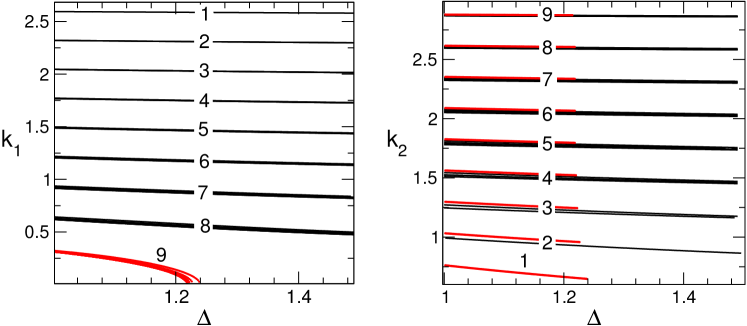
Figure 8: Same as in Figure 7, now shown for a larger chain ($L=12$). There are $\frac{1}{2}(L-3)(L-4)$ solutions of {Re,Re} type at $\Delta$ values above the exceptional points (consistent with Table 1) and $\frac{1}{2}(L-2)(L-3)$ such solutions at small $\Delta$.

The same scenario outlined so far is observed at larger $L$. In Figure 8 we show the real Bethe momentum pairs $(k_{1},k_{2})$ for a chain with $L=12$. The same qualitative result as in Figure 7 is found. Also, one has $\Delta_{e,1}^{(rr)}<\Delta_{e,2}^{(rr)}<\dots<\Delta_{e,L-3}^{(rr)}\approx 1.2$, i.e. the exceptional points are nearer to the isotropic point $\Delta=1$ (compared to $L=6$), suggesting that $\Delta^{(rr)}_{e,\ell}\to 1\,\forall\,\ell$ in the limit $L\to\infty$ (as proven in section 3 for the single particle sector).

5.2 The exceptional points

As in the one particle case (Section 3), the positions of the exceptional points and the behavior of the Bethe momenta in their vicinity can be characterized analytically. We verified that the momentum pairs $(k_{1},k_{2})$ disappearing at the exceptional points exhibit the behavior

$$k_{1}=(\Delta-\Delta_{e})^{1/2}+{\mathcal{O}}(\Delta-\Delta_{e})\qquad k_{2}=\bar{k}+{\mathcal{O}}(\Delta-\Delta_{e})$$ (29)

as $\Delta\to\Delta_{e}$. Here $\Delta_{e}$ denotes a generic exceptional point $\Delta^{(rr)}_{e,\ell}$ ($\ell=1,2,\dots,L-3$). Note that one has from (29) that $k_{1}$ is vanishing while $k_{2}$ assumes the finite value $\bar{k}$ at $\Delta_{e}$. Moreover, (29) holds on both sides of the exceptional point). The square root behavior as $(\Delta-\Delta_{e})^{1/2}$ reflects the transformation from real to pure imaginary of the momentum $k_{1}$, i.e., the edge-locking transformation.

After substituting (29) in the Bethe equations, one obtains that $\bar{k},\Delta_{e}$ are determined by a set of coupled equations as

$$\cos\bar{k}=\frac{-1+\Delta_{e}+2\Delta_{e}^{2}-4\Delta_{e}^{3}+L(\Delta_{e}-1)(1+2(\Delta_{e}-1)\Delta_{e})}{1+L+\Delta_{e}-3L\Delta_{e}+2(L-2)\Delta_{e}^{2}}$$ (30)

$$e^{2i\bar{k}L}\frac{(e^{i\bar{k}}-\Delta_{e})^{2}}{(e^{-i\bar{k}}-\Delta_{e})^{2}}-\frac{(1+e^{i\bar{k}}-2e^{i\bar{k}}\Delta_{e})^{2}}{(1+e^{-i\bar{k}}-2\Delta_{e}e^{-i\bar{k}})^{2}}=0$$ (31)

5.3 Expansion of the real Bethe momenta in the Ising limit ($\Delta\gg 1$)

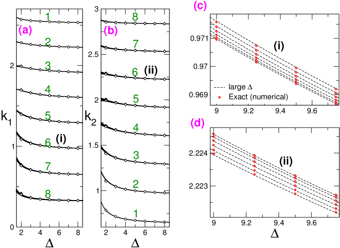
Figure 9: Solutions of {Re,Re} type: large $\Delta$ behavior of the real momentum pairs $(k_{1},k_{2})$. Data for $L=12$. Symbols are numerical solutions of the Bethe equations, and lines are the analytic expansion in the large $\Delta$ regime. (a,b) The number of momenta in each band is shown with the accompanying numbers. (c,d) Zoomed-in comparison between exact numerical solutions of the Bethe equations (symbols) and the large $\Delta$ result (dashed lines) for the momenta in the $k_{1}$ band marked as (i) in panel (a) and for the momenta in the $k_{1}$ band marked as (ii) in panel (b).

We now discuss the {Re,Re} solutions in the large $\Delta$ regime.

Guided by the observation that at $\Delta\gg 1$ the Bethe momenta are “quantized” in units of $\pi/(L-2)$ (Figure 6(a)), and assuming analytic behavior at finite $\Delta$, one can expand as

$$k_{s}=k_{s}^{0}(J_{s})+\sum\limits_{m=1}^{\infty}a_{s,m}(J_{s})\Delta^{-m},\qquad s=1,2$$ (32)

with $k^{0}_{s}$ the zeroth order Bethe momentum given as $k^{0}_{s}\equiv\pi/(L-2)J_{s}$, $J_{s}=1,2,\dots,L-3$ being the Bethe quantum numbers (cf. Figure 6 (a)). The parameters $a_{s,m}$ are determined by substituting (32) in the Bethe equations and equating the coefficients of the same powers of $1/\Delta$. One can readily obtain the large $\Delta$ expansion of the Bethe momenta up to ${\mathcal{O}}(\Delta^{-4})$ as

$$k_{1}=k^{0}_{1}+\frac{3}{\Delta(L-2)}\sin k^{0}_{1}+\frac{1}{\Delta^{2}}\frac{((8+5L)\cos k_{1}^{0}+(L-2)\cos k_{2}^{0})\sin k_{1}^{0}}{2(L-2)^{2}}+$$

$$\frac{1}{4\Delta^{3}(L-2)^{3}}\Big{[}\frac{1}{2}\Big{(}15-21L+2(L-2)(L+1)\cos 2k_{2}^{0}\Big{)}\sin k_{1}^{0}+$$ (33)

$$\frac{3}{2}(L+1)(5+2L)\sin 3k_{1}^{0}+(L-2)(L+4)\cos k_{2}^{0}\sin 2k_{1}^{0}\Big{]}+{\mathcal{O}}(\Delta^{-4})$$

The expression for $k_{2}$ is obtained exchanging $1\leftrightarrow 2$ in (5.3). The expansion (5.3) confirms that at the lowest order in $1/\Delta$ the two particles (magnons) are non interacting, whereas interactions start contributing with terms $\sim 1/(L\Delta)$.

The large $\Delta$ expansion (5.3) is checked in Figure 9 against exact numerical solutions of the Bethe equations, for a $L=12$ chain. For $\Delta\gtrsim 2$, Eq. (5.3) reproduces not only the overall behavior of each band, panels (a,b), but also the fine structure within the bands, panels (c,d).

6 Fully edge-locked states: pure imaginary momentum pairs

In this section we focus on the pure imaginary momentum pairs $(k_{1}\equiv i\kappa_{1},k_{2}\equiv i\kappa_{2})$ (type $\{\textrm{Im},\textrm{Im}\}$, three states in the last row of Table 1). These correspond to eigenstates of (1) with both particles locked at the edges of the chain.

Figure 10 plots all the imaginary momentum pairs (their imaginary parts $\kappa_{1},\kappa_{2}$) as function of the anisotropy $\Delta$ for a chain with $L=6$ sites. Data are numerical solutions of the Bethe equations. The two components of a given momentum pair are shown with the same symbols.

Clearly in the large $\Delta$ ($\Delta\gtrsim 2.1$) there are three pure imaginary momentum pairs (cf. Table 1). Two of them (that we denote as ${\mathbf{k}}_{\pm}$, respectively rhombi and triangles in the Figure) are “degenerate” at $\Delta\to\infty$, meaning that ${\mathbf{k}}_{+}\equiv(i\kappa_{+,1},i\kappa_{+,2})\to{\mathbf{k}}_{-}\equiv(i\kappa_{-,1},i\kappa_{-,2})$. On the other hand the “isolated” one (${\mathbf{k}}_{0}$, circles in the Figure) is a pair of two quasi-degenerate momenta in the limit $\Delta\to\infty$.

At lower $\Delta$ one has two exceptional points $\Delta_{e,1}^{(ii)},\Delta^{(ii)}_{e,2}$ at which one component of a pure imaginary pair vanishes. Precisely, this occurs at $\Delta_{e,2}^{(ii)}\approx 1.9$ for ${\mathbf{k}}_{0}$ and at $\Delta_{e,1}^{(ii)}\approx 1.2$ for ${\mathbf{k}}_{-}$. Note that ${\mathbf{k}}_{+}$ survives up to the isotropic point ($\Delta=1$) where both its components are vanishing (i.e. $\Delta=1$ is also an exceptional point). The vanishing momenta at $\Delta\gtrsim\Delta^{(ii)}_{e,\ell}$ emerge on the other side of the exceptional point (at $\Delta\lesssim\Delta^{(ii)}_{e,\ell}$) as real momenta, i.e. the transformation $\{\textrm{Im},\textrm{Im}\}\to\{\textrm{Re},\textrm{Im}\}$ occurs. This reflects the delocalization of one of the two edge-locked particles, which becomes extended (magnon-like).

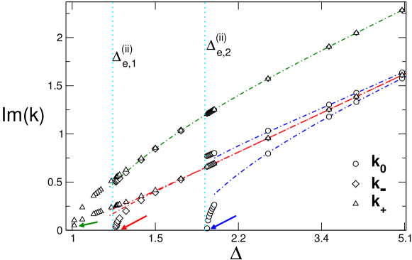
Figure 10: The three solutions of {Im,Im} type, denoted ${\mathbf{k}}_{\pm}$, ${\mathbf{k}}_{0}$, for an $L=6$ chain. Momenta forming a pair are denoted with the same symbols. At large $\Delta$ the pairs ${\mathbf{k}}_{\pm}$ are “degenerate”. At the exceptional point $\Delta=\Delta_{e,2}^{(ii)}$ ($\Delta_{e,1}^{(ii)}$) one of the two momenta forming the pair ${\mathbf{k}}_{0}$ (${\mathbf{k}}_{-}$) vanishes and the {Im,Im} solution disappears. In the limit $\Delta\to 1$ (isotropic point) both the components of ${\mathbf{k}}_{0}$ are vanishing, i.e. no pure imaginary pairs remain at the isotropic point. Dashed-dotted lines are the analytic expansions at large $\Delta$, Eqs. (36),(37),(38).

Both the behaviors around the exceptional points and in the large $\Delta$ region can be understood analytically. It is convenient to parametrize the imaginary Bethe momenta as $z_{i}\equiv e^{\kappa_{i}}$. Now the Bethe equation for $z_{1}$ reads

$$(z_{1}-\Delta)^{2}(z_{1}+z_{2}-2\Delta)(1+z_{1}z_{2}-2z_{2}\Delta)+$$ (34)

$$\qquad\qquad(1-z_{1}\Delta)^{2}(2\Delta z_{2}z_{1}-z_{1}-z_{2})(1+z_{1}z_{2}-2\Delta z_{1})z_{1}^{-2L}=0$$

The equation for $z_{2}$ is obtained from (34) by exchanging $z_{1}\leftrightarrow z_{2}$. Due to the restriction $\kappa_{i}>0$ (Section 2), one has $z_{i}>1$, implying that for large $L$ the second term in (34) is vanishing exponentially. From the first term in (34) one then has $z_{1}=z_{2}=\Delta$ and $z_{1}=2z_{2}=2\Delta$ as possible solutions. The former gives the solution ${\mathbf{k}}_{0}\sim(i\log\Delta,i\log\Delta)$, whereas the latter corresponds to the quasi-degenerate pairs ${\mathbf{k}}_{+}\sim{\mathbf{k}}_{-}\sim(i\log\Delta+i\log 2,i\log\Delta)$. Expansions valid up to higher orders in $\Delta^{-L}\ll 1$ are given in the next subsection.

6.1 The imaginary momentum pairs at large $\Delta$

In this section we investigate the fine structure of the pure imaginary momentum pairs $\mathbf{k}_{\pm}$, $\mathbf{k}_{0}$ at large $\Delta$. The small parameter for the expansion is $\Delta^{-L}$, so that this can also be interpreted as a large $L$ expansion.

We start with the solution $\mathbf{k}_{0}$ (Figure 10). The idea is to expand the two members of the imaginary pair as

$$z^{(0)}_{i}=\Delta+\sum\limits_{m=0}^{\infty}\frac{b_{i,m}}{\Delta^{L/2-2+m}},\qquad i=1,2$$ (35)

where the superscript in $z_{i}^{(0)}$ is to stress that we are focusing on the pair ${\mathbf{k}}_{0}$. The coefficients $b_{i,m}$ are determined by substituting (35) in the Bethe equations (34) and solving the linear system obtained equating the coefficients of the same powers in $1/\Delta$. After a lengthy algebra the first two non trivial orders of $z^{(0)}_{1},z^{(0)}_{2}$ are obtained as

$$z^{(0)}_{1}=\Delta+\frac{\Delta^{2}}{(L-3)^{\frac{1}{4}}\Delta^{L/2}}-\frac{3(L-4)}{[3+(-1)^{L/2-2}]2^{[1-(-1)^{L/2}]/2}(L-3)^{\frac{5}{4}}\Delta^{L/2}}+o(\Delta^{-L/2})$$ (36)

$$z^{(0)}_{2}=\Delta-\frac{\Delta^{2}}{(L-3)^{\frac{1}{4}}\Delta^{L/2}}+\frac{3(L-4)}{[3+(-1)^{L/2-2}]2^{[1-(-1)^{L/2}]/2}(L-3)^{\frac{5}{4}}\Delta^{L/2}}+o(\Delta^{-L/2})$$

where $o(\Delta^{-L/2})$ denotes higher order corrections. One should stress that the expansion (36) does not hold if the size of the chain is too small. For example, we find that for $L=6$ one has, instead of (36), the expansion

$$z^{(0)}_{1}=\Delta+\frac{1}{3^{1/4}\Delta}-\frac{6+3^{1/4}}{2\cdot 3^{1/2}\Delta^{3}}+o(\Delta^{-3})$$ (37)

$$z^{(0)}_{2}=\Delta-\frac{1}{3^{1/4}\Delta}+\left(3^{1/2}-2\cdot 2^{1/2}+\frac{1}{2\cdot 3^{1/4}}\right)\frac{1}{\Delta^{3}}+o(\Delta^{-3})$$

While the first two orders in (37) for both $z_{1}^{(0)}$ and $z_{2}^{(0)}$ are correctly reproduced by the general result (36), this is not the case for the last order $\sim\Delta^{-3}$.

A similar expansion can be carried out for the case of the two almost “degenerate” (at $\Delta\to\infty$) pairs ${\mathbf{k}}_{\pm}$ (cf. Figure 10). The first few orders for the corresponding $z^{(\pm)}_{\ell}$ are given as

$$z^{(+)}_{1}=\Delta+\frac{1}{2^{L-3}\Delta^{2L-5}}+o(\Delta^{-2L+5}) \qquad z_{2}^{(+)}=2\Delta-\frac{1}{\Delta}-\frac{1}{(2\Delta)^{2L-5}}+o(\Delta^{-2L+5})$$ (38)

$$z^{(-)}_{1}=\Delta+\frac{1}{2^{L-3}\Delta^{2L-5}}+o(\Delta^{-2L+5}) \qquad z_{2}^{(-)}=2\Delta-\frac{1}{\Delta}+\frac{1}{(2\Delta)^{2L-5}}+o(\Delta^{-2L+5})$$

Note that the higher order corrections decay faster (as $o(\Delta^{-2L+5})$) than in the case of ${\mathbf{k}}_{0}$ (as $o(\Delta^{-L/2})$).

The validity of the expansions (36),(37),(38) for all pairs ${\mathbf{k}}_{0},{\mathbf{k}}_{\pm}$ is checked against exact results obtained by solving the Bethe equations numerically in Figure 10. It is remarkable that the agreement between the exact data and the expansions is good even in the region $\Delta\approx 1$. Deviations are only visible near the exceptional points, where Eqs. (36),(37),(38) are inadequate.

6.2 Expansion of the imaginary pairs near the exceptional points

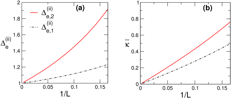
Figure 11: (a) Exceptional points $\Delta_{e,1}^{(ii)}$ and $\Delta^{(ii)}_{e,2}$ as function of inverse chain length $1/L$. Both points coalesce at $\Delta=1$ at large $L$. (b) The value $\bar{\kappa}$ of the non vanishing imaginary momentum at the exceptional point. For both cases $\bar{\kappa}\to 0$ at large $L$.

The two exceptional points $\Delta_{e,\ell}^{(ii)}$ at which the pure imaginary solutions of the Bethe equations for two particles disappear are obtained by imposing that the imaginary momentum pair is of the form

$$k_{1}=i(\Delta-\Delta_{e})^{1/2}+{\mathcal{O}}(\Delta-\Delta_{e}),\qquad k_{2}=i\bar{\kappa}+{\mathcal{O}}(\Delta-\Delta_{e})$$ (39)

with $\Delta_{e}$ and $\bar{\kappa}$ respectively the exceptional point and the imaginary value of $k_{2}$ at $\Delta_{e}$. Eq. (39) is valid on both sides of the exceptional point. It encodes the transformation {Im,Im} $\to$ {Re,Im}, i.e., the fact that $k_{1}$ is imaginary for $\Delta>\Delta_{e}$ and real for $\Delta<\Delta_{e}$. The two parameters $\Delta_{e}$ and $\bar{\kappa}$ are determined by solving the coupled equations

$$\cosh\bar{\kappa}=\frac{-1+\Delta_{e}+2\Delta_{e}^{2}-4\Delta_{e}^{3}+L(\Delta_{e}-1)(1+2(\Delta_{e}-1)\Delta_{e})}{1+L+\Delta_{e}-3L\Delta_{e}+2(L-2)\Delta_{e}^{2}}$$ (40)

$$e^{-2\bar{\kappa}L}\frac{(e^{-\bar{\kappa}}-\Delta_{e})^{2}}{(e^{\bar{\kappa}}-\Delta_{e})^{2}}=\frac{(1+e^{-\bar{\kappa}}-2\Delta_{e}e^{-\bar{\kappa}})^{2}}{(1+e^{\bar{\kappa}}-2\Delta_{e}e^{\bar{\kappa}})^{2}}$$ (41)

Clearly, Eqs. (40), (41) can be obtained from Eqs. (30), (31) by redefining $\bar{k}\to i\bar{\kappa}$.

It is interesting to investigate the behavior of the exceptional points $\Delta_{e}^{(ii)}$ and “amplitude” $\bar{\kappa}$, solutions of (40) (41), as function of chain size $L$ (Figure 11). In the $L\to\infty$ limit, $\Delta_{e,1}^{(ii)}\to 1$ and $\Delta_{e,2}^{(ii)}\to 1$. Also, $\bar{\kappa}\to 0$ for large chains.

6.3 Fully edge-locked two-particle eigenfunctions

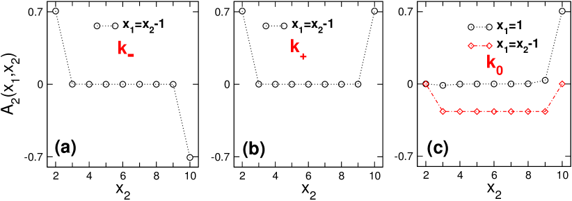
Figure 12: Edge-locked eigenfunctions corresponding to the {Im,Im} type solutions ($\mathbf{k}_{-}$, $\mathbf{k}_{+}$, $\mathbf{k}_{0}$). Data for $L=10$ chain at $\Delta=20$. The eigenfunction components $A_{2}(x_{1},x_{2})$ as function of $x_{2}$, the position of the second particle. Only the components which are significantly nonzero are shown. (a) The eigenfunction obtained from the solution ${\mathbf{k}}_{-}$: $A_{2}(x_{2}-1,x_{2})$ against $x_{2}$. (b) Same as in (a) but for the solution ${\mathbf{k}}_{+}$. (c) The eigenfunction amplitude obtained from ${\mathbf{k}}_{0}$: $A_{2}(1,x_{2})$ (circles) and $A_{2}(x_{2}-1,x_{2})$ (rhombi). In contrast to $\mathbf{k}_{\pm}$, this eigenfunction contains non-negligible bulk contributions, c.f. Eq. (43).

In this section we discuss the edge-locked nature of the pure imaginary solutions of the Bethe equations by constructing explicitly the corresponding eigenfunctions. In Figure 12 we show for each of the three {Im,Im} solutions $\mathbf{k}_{\pm}$, $\mathbf{k}_{0}$ the corresponding eigenvector components $A_{2}(x_{1},x_{2})$, i.e., the amplitudes of the configurations with particles at positions $x_{1}<x_{2}$. Data are obtained by solving numerically the Bethe equations for a chain with $L=10,\Delta=20$. We consider only the configurations leading to significantly non zero amplitudes. For instance one has that the eigenvectors $|\psi_{\pm}\rangle$ corresponding to ${\mathbf{k}}_{\pm}$ are well approximated by

$$|\psi_{\pm}\rangle\leavevmode\nobreak\ \approx\leavevmode\nobreak\ \frac{1}{\sqrt{2}}(|1,2\rangle\pm|L-1,L\rangle)$$ (42)

with $|1,2\rangle,|L-1,L\rangle$ denoting the configurations with the two particles at positions $1,2$ and $L-1,L$ (respectively the first two and last two sites in the chain). Note that the two eigenfunctions correspond to states with opposite parity under ${\mathcal{I}}:i\to L-i+1$ (inversion with respect to the center of the chain).

The eigenvector obtained from ${\mathbf{k}}_{0}$ (cf. Figure 12 (c)) is symmetric under ${\mathcal{I}}$ and is well approximated (in the large $\Delta$ regime) by

$$|\psi_{0}\rangle\leavevmode\nobreak\ \approx\leavevmode\nobreak\ \frac{1}{\sqrt{2}}|1,L\rangle\leavevmode\nobreak\ -\leavevmode\nobreak\ \frac{1}{\sqrt{2(L-3)}}\sum\limits_{m=2}^{L-2}|m,m+1\rangle$$ (43)

Physically, $|\psi_{0}\rangle$ is a superposition of a pure edge-locked contribution and a bulk one. The latter is an equal weight superposition of the configurations with the two particles next to each other, i.e., a delocalized bound state. The delocalized part is reminiscent of a string solution with vanishing momentum (Section 8). The edge-locked part of the wavefunction has on particle on either edge; there is no significant contribution from the configuration with both particles on the same edge.

7 Coexistence of extended and edge locked behavior: the {Re,Im} momentum pairs

In this section we examine the $M=2$ solutions with one real and one imaginary Bethe momentum. Clearly, the presence of the imaginary momentum signals edge-locking behavior for one particle, while the real momentum signals that the other particle is extended (magnon-like). The total number of such eigenstates at large $\Delta$ is given as $2(L-3)$ (Table 1) and corresponds to the total number of configurations with only one particle localized at one edge of the chain and the constraint that two particles cannot be on nearest-neighbor sites.

As $\Delta$ is lowered, exactly half of the {Re,Im} soutions turn into {Re,Re} solutions at $L-3$ exceptional points. The exceptional points are the same as those discussed in Section 5 ($\Delta^{(rr)}_{e,\ell}$; $\ell=1,2,\dots,L-3$) where $L-3$ extra {Re,Re} solutions at small $\Delta$ vanish as $\Delta$ is increased. In other words, the vanishing {Re,Re} solutions observed in Figures 7 and 8 reappear as {Re,Im} on the other (larger) side of $\Delta^{(rr)}_{e,\ell}$. The location of the exceptional points and the value of the other momentum at these points are therefore given by the nonlinear equations (30), (31).

This scenario is illustrated in Figure 13 by plotting all the momentum pairs of type $\{\textrm{Re},\textrm{Im}\}$ for a $M=2$, $L=6$, chain. The imaginary and real components of the generic pair are denoted as $\kappa_{1}$ and $k_{2}$. While in the large $\Delta$ region there are $2(L-3)=6$ momentum pairs, only half of them (i.e. $L-3$) are present near the Heisenberg point $\Delta=1$. The other solutions disappear at the exceptional points $\Delta_{e,\ell}^{(rr)}$ ($\ell=1,2,3$), which are the same as in Figure 7. It is worth mentioning that the $L-3$ states surviving across the exceptional points undergo the transformation $\{\textrm{Re},\textrm{Im}\}\to\{\textrm{Re},\textrm{Re}\}$ at $\Delta=1$, as can be surmised from the vanishing of $\kappa_{1}$ at $\Delta\to 1$ in Figure 13(b).

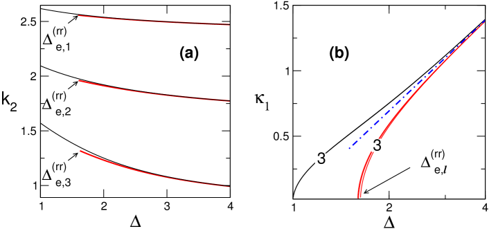
Figure 13: One real and one imaginary momentum, $(i\kappa_{1},k_{2})$ ($\kappa_{1},k_{2}\in{\mathbb{R}}$), of solutions of {Re,Im} type. Numerical solution of Bethe equations, for a $L=6$ chain, $1\leq\Delta\leq 4$. There are $2(L-3)$ such solutions at large $\Delta$ and $(L-3)$ such solutions at small $\Delta$. (a) The real momentum $k_{2}$ versus $\Delta$: the $L-3=3$ bands of solutions (two solutions per band). The arrows denote the exceptional points $\Delta_{e,\ell}^{(rr)}$ ($\ell=1,2,3$) at which $L-3$ solutions (one per band) disappear; these re-emerge as {Re,Re} solutions at smaller $\Delta$ below $\Delta_{e,\ell}^{(rr)}$. The exceptional points are therefore the same as in Figure 7. (b) The pure imaginary momentum $i\kappa_{1}$ of the pair. The $\Delta$ axis is in logarithmic scale. At the exceptional points $L-3$ pure imaginary momenta vanish. The dashed-dotted line is the large $\Delta$ behavior, $\sim\log\Delta$.

Bethe equations for {Re,Im} solutions.

We define $(k_{1},k_{2})\to(i\kappa_{1},k_{2})$, with $\kappa_{1},k_{2}$ real. The Bethe equations become

$$e^{-2(L+1)\kappa_{1}}\frac{(1-\Delta e^{\kappa_{1}})^{2}}{(1-\Delta e^{-\kappa_{1}})^{2}}=\frac{(1+e^{ik_{2}-\kappa_{1}}-2\Delta e^{-\kappa_{1}})(1+e^{ik_{2}+\kappa_{1}}-2\Delta e^{ik_{2}})}{(1+e^{ik_{2}-\kappa_{1}}-2\Delta e^{ik_{2}})(1+e^{ik_{2}-\kappa_{1}}-2\Delta e^{\kappa_{1}})}$$ (44)

$$e^{i2(L+1)k_{2}}\frac{(1-\Delta e^{-ik_{2}})^{2}}{(1-\Delta e^{ik_{2}})^{2}}=\frac{(1+e^{ik_{2}-\kappa_{1}}-2\Delta e^{ik_{2}})(1+e^{-ik_{2}-\kappa_{1}}-2\Delta e^{-\kappa_{1}})}{(1+e^{ik_{2}-\kappa_{1}}-2\Delta e^{-\kappa_{1}})(1+e^{-ik_{2}-\kappa_{1}}-2\Delta e^{-ik_{2}})}$$ (45)

which, after redefining $z_{1}\equiv e^{\kappa_{1}}$, read

$$\frac{(1-\Delta z_{1})^{2}}{z_{1}^{2L}(z_{1}-\Delta)^{2}}=\frac{(1+e^{ik_{2}}/z_{1}-2\Delta/z_{1})(1+z_{1}e^{ik_{2}}-2\Delta e^{ik_{2}})}{(1+e^{ik_{2}}/z_{1}-2\Delta e^{ik_{2}})(1+e^{ik_{2}}z_{1}-2\Delta z_{1})}$$ (46)

$$e^{i2(L+1)k_{2}}\frac{(1-\Delta e^{-ik_{2}})^{2}}{(1-\Delta e^{ik_{2}})^{2}}=\frac{(1+e^{ik_{2}}/z_{1}-2\Delta e^{ik_{2}})(1+e^{-ik_{2}}/z_{1}-2\Delta/z_{1})}{(1+e^{ik_{2}}/z_{1}-2\Delta/z_{1})(1+e^{-ik_{2}}/z_{1}-2\Delta e^{-ik_{2}})}$$ (47)

We focus on the denominator of the left side in (46), considering large $\Delta$ and $L$. Using $z_{1}>1$ one has that the term $z_{1}^{2L}$ grows exponentially with $L$. The right side of (46) shows a different behavior (it vanishes mildly with increasing $L$) unless $z_{1}=\Delta+e^{-\beta L}$ with $\beta>0$. After fixing $z_{1}=\Delta$ the degree of freedom of one particle is “frozen” (the particle is edge locked) and the Bethe like equation for the momentum $k_{2}$ of the “free” (i.e. not locked) one is given as

$$e^{i2(L+1)k_{2}}=\frac{(1+e^{ik_{2}}/\Delta-2\Delta e^{ik_{2}})(1-e^{-ik_{2}}/\Delta)(1-\Delta e^{ik_{2}})^{2}}{(1+e^{-ik_{2}}/\Delta-2\Delta e^{-ik_{2}})(1-e^{ik_{2}}/\Delta)(1-\Delta e^{-ik_{2}})^{2}}$$ (48)

Taking the logarithm of both sides of (48) one has

$$(L+1)k_{2}\leavevmode\nobreak\ =\leavevmode\nobreak\ \pi J_{\alpha}+\arctan\frac{\sin k_{2}}{\Delta-\cos k_{2}}\leavevmode\nobreak\ -$$ (49)

$$\qquad 2\arctan\frac{\Delta\sin k_{2}}{1-\Delta\cos k_{2}}+\arctan\frac{(1-2\Delta^{2})\sin k_{2}}{\Delta+(1-2\Delta^{2})\cos k_{2}}$$

Numerically, we find that Eq. (49) admits $(L-3)$ real solutions for $k_{2}$, which are obtained choosing the Bethe numbers as $J_{\alpha}=\{1,2,\dots,\lfloor(L-3)/2\rfloor\}\cup\{L-\lceil(L-3)/2\rceil+1,\dots,L\}$. Each solution of (49) has to be counted with a degeneracy factor two, in order to recover the correct counting $2(L-3)$. In fact, including the higher order corrections in (46), i.e., going beyond the approximation $z_{1}\sim\Delta$, has the effect of splitting in two every solution of (49). The splitting vanishes exponentially with $L$, implying that for large enough $L$ the solutions of (49) (with $\kappa_{1}=\log\Delta$) coincide, in practice, with the solutions of (46), (47).

8 Bound state of two delocalized particles: string solutions

We now discuss the solutions of the Bethe equations which are complex conjugate pairs (“strings”), which describe eigenstates where the two particles are mutually bound and spatially extended. While other classes of solutions (cf. Table 1) change nature upon changing the anisotropy $\Delta$, it turns out that all the string solutions are stable in the whole region $\Delta\in(1,\infty)$, i.e., there is no unbinding of the pair at any $\Delta>1$.

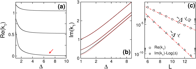
Figure 14: String solutions $(k_{2}\equiv k_{1}^{*})$ representing bound delocalized states. Data for a $L=6$ chain. Note that the number of string solutions ($L-3$) does not change with $\Delta$ (no exceptional points). (a) Real part of $k_{1}$ as a function of $\Delta$. The $\Delta\to\infty$ asymptotic values are described by (55). The lowest solution (marked by the arrow) shows vanishing momentum. (b) Imaginary part of $k_{1}$ as function of $\Delta$. The asymptotic behavior is given as $\log[\Delta/\cos(\textrm{Re}(k_{1}))]$ (dotted lines). (c) The string with vanishing real part (c.f. panel (a)): $\textrm{Re}\,(k_{1})$ and $\textrm{Im}\,(k_{1})-\log\Delta$ as function of the chain size $L$ at fixed $\Delta=10$. Dashed-dotted lines are fits to $\sim\Delta^{-L/2}$ and $\sim\Delta^{-L}$.

After defining $k_{1}=a+ib$ and $k_{2}=a-ib$, and using the parametrization $z\equiv e^{b}$, the Bethe equations read

$$e^{i2(L+1)a}/z^{2(L+1)}=\frac{(1-\Delta e^{ia}/z)^{2}(1+e^{2ia}-2\Delta e^{ia}/z)(1+z^{2}-2\Delta e^{ia}z)}{(1-\Delta e^{-ia}z)^{2}(1+e^{2ia}-2\Delta e^{ia}z)(1+z^{2}-2\Delta e^{-ia}z)}$$ (50)

$$e^{i2(L+1)a}z^{2(L+1)}=\frac{(1-\Delta e^{ia}z)^{2}(1+e^{2ia}-2\Delta e^{ia}z)(1+1/z^{2}-2\Delta e^{ia}/z)}{(1-\Delta e^{-ia}/z)^{2}(1+e^{2ia}-2\Delta e^{ia}/z)(1+1/z^{2}-2\Delta e^{-ia}/z)}$$ (51)

which can be rewritten as

$$\frac{(z\cos a-\Delta)(1+z^{2}-2z\Delta e^{ia})}{z(z\Delta-\cos a)(1+z^{2}-2z\Delta e^{-ia})}+z^{-2L}e^{2iLa}\frac{(1-z\Delta e^{-ia})^{2}}{(\Delta-ze^{-ia})^{2}}=0$$ (52)

$$\frac{z(z\Delta-\cos a)(1+z^{2}-2z\Delta e^{ia})}{(z\cos a-\Delta)(1+z^{2}-2z\Delta e^{-ia})}+z^{2L}e^{2iLa}\frac{(\Delta-ze^{ia})^{2}}{(1-z\Delta e^{ia})^{2}}=0$$ (53)

We observe that the second term in equation (52), [(53)] vanishes [diverges] exponentially with $L\to\infty$ if the imaginary part of the momentum (i.e. $b$) is negative [positive]. In order to match the behavior of the two terms one can impose $z\sim\Delta/\cos a$, neglecting (additive) exponentially vanishing contributions in the limit $L\to\infty$. After fixing $z=\Delta/\cos a$ in (52), (53), and multiplying the two Bethe equations to cancel the vanishing denominator in (53) one obtains

$$\frac{(1+e^{2ia}-2\Delta e^{2ia})^{2}(1+e^{2ia}+2\Delta e^{2ia})^{2}}{(1+e^{-2ia}-2\Delta e^{-2ia})^{2}(1+e^{-2ia}+2\Delta e^{-2ia})^{2}}=e^{4ia(L+3)}\frac{(1+e^{-2ia}-2\Delta^{2}e^{-2ia})^{2}}{(1+e^{2ia}-2\Delta^{2}e^{2ia})^{2}}$$ (54)

or in logarithmic form

$$(L+3)a=\pi J+\arctan\frac{(1-2\Delta^{2})\sin(2a)}{1+(1-2\Delta^{2})\cos(2a)}+$$ (55)

$$\qquad\arctan\frac{(1-2\Delta)\sin(2a)}{1+(1-2\Delta)\cos(2a)}+\arctan\frac{(1+2\Delta)\sin(2a)}{1+(1+2\Delta)\cos(2a)}$$

The equation above is similar to the so-called Bethe-Takahashi equations [28, 29, 30, 31] that appear in the study of string solutions in the XXZ chain with periodic boundary conditions.

The quantum numbers $J\in[1,L]$ identify the different solutions of (55). Note that there is a subtlety in equation (55): the number of real solutions is found numerically to be $L-4$. To get the correct number of strings ($L-3$) from these leading-order large-$L$ equations, one should include the solution $a=0$ (which implies $z\to\log\Delta$). Higher order corrections to $z$, going beyond $z\sim\Delta/\cos a$, would make this solution non vanishing.

Interestingly, this implies that the string solution with $a\to 0$ is almost degenerate in energy with one of the edge-locked states, namely, the edge-locked eigenstate obtained from the momentum pair ${\bf k}_{0}$ of Figure 10. Figure 14(a) and Figure 15 highlight this string solution with red arrows.

All these findings are supported numerically in Figure 14 plotting the momenta $k_{1}$ $k_{2}$ for all the string solutions for a chain with $L=6$ as function of the anisotropy $1<\Delta<10$ (plot of $\textrm{Re}(k_{1})=a$ and $\textrm{Im}(k_{1})=b$, respectively panels (a) and (b) in Figure 14). Data are obtaining by solving numerically the Bethe equations. In Figure 14 (a) the arrow denotes the string solution with vanishing real part. Figure 14 (b) shows the imaginary parts of the string solutions (continuous lines is $\textrm{Im}(k_{1})$ versus $\Delta$). The dotted lines is $\log(\Delta/\cos\textrm{Re}(k_{1}))$, where for $\textrm{Re}(k_{1})$ the values reported in panel (a) are used.

The difference between $\textrm{Im}(k_{1})$ and $\log(\Delta/\cos\textrm{Re}(k_{1}))$ is not visible, except for the lowest curve, especially at large $\Delta$. More information about the string with vanishing momentum is shown in panel (c) plotting both $\textrm{Re}(k_{1})$ and $\textrm{Im}(k_{1})-\log\Delta$ versus $L$ at fixed $\Delta=10$ (logarithmic scale on the $y$-axis). Clearly deviations from the asymptotic (i.e. at large $L$) solution $\textrm{Im}(k_{1})=i\log\Delta,\textrm{Re}(k_{1})=0$ decay exponentially with increasing $L$.

9 The two-particle energy spectrum: edge-locking vs extended behavior

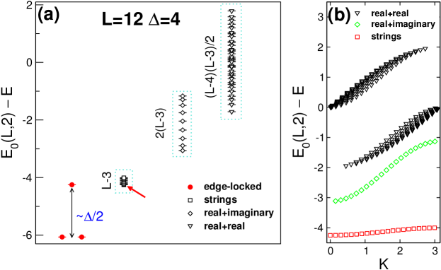
Figure 15: Energy spectrum of the open XXZ spin chain in the sector with two particles, inverted and added to $E_{0}(L,2)\equiv\frac{1}{4}(L-9)\Delta$. Data shown for a $L=12$ chain at $\Delta=4$. (a) The four types of eigenstates are separated horizontally, the $x$-axis is otherwise a dummy axis. The lowest three levels are the edge-locked states ({Im,Im} solutions). The total number of energy levels for each type of solution is also shown. The lowest energy level in the string sector (arrow) is almost degenerate with one of the edge-locked states. The levels of {Re,Im} type are almost doubly degenerate. (b) Dispersion of the different types of eigenstates, plotted as the energy versus the total real momentum $K\equiv\mathrm{Re}(k_{1})+\mathrm{Re}(k_{2})\,[\mathrm{mod}\,\pi]$.

In this section we analyze the full two-particle energy spectrum of the open-boundary XXZ spin chain, at anisotropies larger than the region of exceptional points. In particular, for each class of solution ({Re,Re}, {Re,Im}, etc) of the Bethe equations we isolate the corresponding contributions to the spectrum. In Figure 15 we show the spectrum for an $L=12$ chain at $\Delta=4$, obtained from numerically solving the Bethe equations. We choose to plot the quantity $E_{0}(L,2)-E$, i.e., the energies are inverted and added to $E_{0}(L,2)\equiv\frac{1}{4}(L-9)\Delta$, so that the fully edge-locked states appear at the bottom.

The lowest three levels (full circles in the Figure) correspond to the edge-locked states. The doublet at the bottom and the isolated level above are given respectively by the half-string solutions ${\mathbf{k}}_{\pm}$ and ${\mathbf{k}}_{0}$ (cf. Figure 10). The leading large-$\Delta$ behaviors are obtained from (36) and (38) as

$$E_{0}(L,2)-E({\mathbf{k}}_{\pm})\sim-\frac{\Delta-3\Delta^{3}}{1-2\Delta^{2}}\sim-\frac{3}{2}\Delta$$ (56)

and

$$E_{0}(L,2)-E({\mathbf{k}}_{0})\sim-\frac{\Delta^{4}-\Delta^{L}\sqrt{L-3}(1+\Delta^{2})}{\Delta^{3}-\sqrt{L-3}\Delta^{1+L}}\sim-\Delta$$ (57)

The lowest dispersing levels above the edge-locked sector are the strings. The lowest level in the string sector, which corresponds to vanishing total Bethe momentum, is degenerate at large $\Delta$ with the edge-locked level obtained from the solution ${\bf k}_{0}$. Higher levels in the spectrum correspond to the {Re,Im} type and the two magnons (type {Re,Re}), which contribute respectively with $2(L-3)$ and $(L-4)(L-3)/2$ energy levels.

In Figure 15(b), $E_{0}(L,2)-E$ is plotted against the total real part of Bethe momenta, $K\equiv\mathrm{Re}(k_{1})+\mathrm{Re}(k_{2})\,[\mathrm{mod}\,\pi]$. For the {Re,Re} type solutions, $k_{1}+k_{2}$ ranges from 0 to $2\pi$, and therefore the {Re,Re} band appears split into two in the $(0,\pi)$ domain.

The width of the dispersion in the string states is smaller compared to the other classes of states and depends on the anisotropy $\Delta$. The dispersion of the string states, using the results in section 8, is obtained at leading order in $1/\Delta$ to be

$$E_{0}(L,2)-E\sim-\Delta-\frac{\cos^{2}(K/2)}{\Delta}$$ (58)

The width $\sim 1/\Delta$ vanishes in the Ising limit $\Delta\to\infty$. Physically, this is because two-particle bound states are “heavy” objects with effective hopping strength $\sim 1/\Delta$ [4, 32]. The dependence of the dispersion with $\Delta$ is different for the other two classes of dispersive solutions ({Re,Re} and {Re,Im}), for which the dispersion width does not change significantly with $\Delta$ and $L$, and is given respectively by $\delta E\sim 4$ and $\delta E\sim 2$.

10 Conclusions: Summary and Perspectives

Summary.

In this Article, we investigated edge-locking behavior in the eigenstates of the spin-$\frac{1}{2}$ Heisenberg XXZ chain with open boundary conditions, in the highly polarized sectors $M=1$ and $M=2$. Exploiting the Bethe ansatz solution of the model we constructed explicitly the full spectrum (energies and eigenfunctions), focusing on the region at $\Delta>1$. We presented a complete classification of all the possible solutions of the Bethe equations in the whole region $\Delta\in(1,\infty)$.

Edge-locked eigenstates are those in which one or more of the particles are exponentially localized at the edges of the chain. In all sectors (e.g., the $M=1$ and $M=2$ sectors we have detailed), there are two eigenstates where the particles are all localized at the left or at the right edge. In addition, for $M>1$ we can have some particles localized at the left edge and some localized at the right edge. These fully edge-locked eigenstates are all associated with pure imaginary solutions of the Bethe equations. In contrast, real solutions of the Bethe equations reflect extended (i.e. “magnon”-like) behavior. For $M>1$, we naturally can have eigenstates where some of the particles are extended and some are edge-localized, i.e., solutions with some momenta real and some momenta imaginary. In the $M=2$ case, these show up as {Re,Im} type of solutions. Finally, for $M>1$ one can also have string solutions with the particles bound but delocalized.

At large $\Delta$, one can use combinatorial counting of different spatial configurations and find out the numbers of eigenstates of different types, i.e., the numbers of real and imaginary solutions in the $M=1$ case (Section 3), and the numbers of {Re,Re}, {Im,Im}, {Re,Im}, and string types of solutions in the $M=2$ case (Section 4).

At any finite chain length $L$, as one decreases $\Delta$, we find that there are special values of $\Delta$ where some of the imaginary momenta pass through zero and become real momenta. In the $M=1$ case, one of the two imaginary solutions becomes real at $\Delta_{e}=\frac{L+1}{L-1}$, so that we are left with a single imaginary solution, i.e., a single edge-locked eigenstate, at $\Delta\in(1,\Delta_{e})$. For $M=2$, we have transitions from {Im,Im} to {Re,Im}, or from {Re,Im} to {Re,Re}, as $\Delta$ is lowered. This corresponds to some of edge-locked particles getting delocalized and becoming extended in the bulk of the chain. We have characterized in detail these changes of eigenstates, the positions of the “exceptional points” where they occur, and the behavior of the Bethe momenta near these points and at large $\Delta$. In the large-chain ($L\to\infty$) limit, the exceptional points all coalesce at the isotropic point $\Delta=1$, so that all the edge-locking present at large $\Delta$ become stable in the whole $\Delta\in(1,\infty)$ region. The string solutions (complex conjugate momentum pairs) are found to be stable with no change of character in the whole $\Delta\in(1,\infty)$ region, even at finite $L$.

We have also presented spectral signatures of edge-locking (Figures 1, 4, 15). At large $\Delta$, in all $M$ sectors, two of the fully edge-locked states are distinctly well-separated from the rest of the spectrum, by a gap $\sim\Delta$. The energy splitting within this doublet vanishes exponentially with the chain length. In the $M=2$ sector, there is an additional edge-locked state which has a $\left|{1,L}\right.\rangle$ component (one particle edge-locked at each edge), and also a string-like component extended in the bulk, c.f., Eq. (43). This new fully edge-locked state is the third state at the bottom of the inverted spectrum and nearly degenerate with the edge of the band of string eigenstates (Figure 15).

Open Issues.

The present work opens up a number of research avenues.

We have focused on the region $\Delta\in(1,\infty)$, where we have detailed the different types of eigenstates and related them to edge-locking, and shown how there are transformations between different types as a function of $\Delta$ and $L$. The intuition at $\Delta\gg{1}$, where spin configuration counting gives accurate classification and counting of the different types of eigenstates, has been particularly helpful. Clearly, the situation should be quite different at the isotropic point, $\Delta=1$, and at smaller anisotropies, $\Delta<1$. Classifying the eigenstates according to their edge behavior for the open XXZ chain in these regimes remains an open task.

We have restricted ourselves to the $M=1$ and $M=2$ sectors, since there was substantial detail to be worked out in these cases. It is known that the $M>2$ sectors contain richer edge-related behavior and novel types of edge-locking phenomena [4]. In particular, for larger $M$, there is a hierarchy of locking behaviors at increasing distances from the edge, related to sub-structures with smaller gaps in the energy spectrum. A Bethe ansatz description of $M>2$ sectors for the open-boundary XXZ chain is thus expected to include a rich set of behaviors beyond those explored in the present study.

References

References

- [1] J. Kondo, Resistance Minimum in Dilute Magnetic Alloys, Prog. Theo. Phys. 32, 37 (1964).
- [2] P. W. Anderson, Infrared Catastrophe in Fermi Gases with Local Scattering Potentials, Phys. Rev. Lett. 18, 1049 (1967).
- [3] R. A. Pinto, M. Haque, S. Flach, Edge-localized states in quantum one-dimensional lattices, Phys. Rev. A 79 052118 (2009).
- [4] M. Haque, Edge-locking and quantum control in highly polarized spin chains, Phys. Rev. A, 82 012108 (2010).
- [5] F. C. Alcaraz, M. N. Barber, M. T. Batchelor, R. J. Baxter and G. R. W. Quispel, Surface exponents of the quantum XXZ, Ashkin-Teller and Potts models, J. Phys. A: Math. Gen. 20 6397 (1987).
- [6] E. K. Sklyanin, Boundary conditions for integrable quantum systems, J. Phys. A: Math. Gen. 21 2375 (1988).
- [7] S. Skorik and H. Saleur, Boundary bound states and boundary bootstrap in the sine-Gordon model with Dirichlet boundary conditions, J. Phys. A: Math. Gen. 28 6605 (1995).
- [8] A. Kapustin and S. Skorik, Surface excitations and surface energy of the antiferromagnetic XXZ chain by the Bethe ansatz approach, J. Phys. A: Math. Gen. 29 1629 (1996).
- [9] C. Matsui, Boundary bound states in the SUSY sine-Gordon model with Dirichlet boundary conditions, arXiv:1205.0912 (2012).
- [10] P. Fendley and H. Saleur, Deriving boundary S matrices, Nuclear Physics B 428 681 (1994).
- [11] A. LeClair, G. Mussardo, H. Saleur, S. Skorik, Boundary energy and boundary states in integrable quantum field theories, Nuclear Physics B 453 581 (1995).
- [12] H. Asakawa and M. Suzuki, On the Hubbard model with boundaries, Physica A 236 376 (1997).
- [13] P. A. de Sa and A. M. Tsvelik, Anisotropic spin- Heisenberg chain with open boundary conditions, Phys. Rev. B 52 3067 (1995).
- [14] Y. Wang, J. Voit, An Exactly Solvable Kondo Problem for Interacting One-Dimensional Fermions, Phys. Rev. Lett. 77 4934 (1996).
- [15] H. Frahm and A. A. Zvyagin, The open spin chain with impurity: an exact solution, Journal of Physics: Condensed Matter 9 9939 (1997).
- [16] P. Schlottmann, A. A. Zvyagin, Kondo impurity band in a one-dimensional correlated electron lattice, Phys. Rev. B 56 13989 (1997).
- [17] Y. Wang, Exact solution of the open Heisenberg chain with two impurities, Phys. Rev. B 56 14045 (1997).
- [18] H. Asakawa, Wave function in the strong coupling limit of the Hubbard open chain, J. Phys. : Cond. Matt. 10 11743 (1998).
- [19] G. Bedürftig and H. Frahm, Spectrum of boundary states in the open Hubbard chain, J. Phys. A: Math. Gen. 30 4139 (1997).
- [20] H. Frahm and S. Ledowski, Boundary states and edge singularities in the degenerate Hubbard chain, J. Phys. : Cond. Matt. 10 8829 (1998).
- [21] M. Bortz and J. Sirker, Boundary susceptibility in the open XXZ-chain, J. Phys. A: Math. Gen. 38 5957 (2005).
- [22] M. I. Dykman and L. F. Santos, Antiresonance and interaction-induced localization in spin and qubit chains with defects, J. Phys. A: Math. Gen. 36 L561 (2003).
- [23] L. F. Santos, Entanglement in quantum computers described by the XXZ model with defects, Phys. Rev. A 67 062306 (2003).
- [24] M. Karbach, G. Muller, Introduction to the Bethe ansatz I, Computers in Physics 11, 36 (1997). M. Karbach, K. Hu, and G. Muller, Introduction to the Bethe ansatz II, Computers in Physics 12, 565 (1998). M. Karbach, K. Hu, and G. Muller, Introduction to the Bethe ansatz III, arxiv:cond-mat/0008018.
- [25] F. H. L. Essler, V. E. Korepin, K. Schoutens, Fine structure of the Bethe ansatz for the spin Heisenberg XXX model, J. Phys. A: Math. Gen. 25 4115 (1992).
- [26] H. Bethe, Zur Theorie der Metalle. I. Eigenwerte und Eigenfunktionen der linearen Atomkette, Z. Phys. 71, 205 (1931).
- [27] V. E. Korepin, N. M. Bogoliubov, A. G. Izergin, Quantum Inverse Scattering Method and Correlation Functions, Cambridge University Press, Cambridge, 1997.
- [28] M. Takahashi, and M. Suzuki, One-Dimensional Anisotropic Heisenberg Model at Finite Temperatures, Prog. Th. Phys. 48, 2187 (1972). M. Takahashi, Thermodynamics of one-dimensional solvable models, Cambridge University Press, Cambridge, 1999.
- [29] A. Ilakovac, M. Kolanovic, S. Pallua, and P. Preste, Violation of the string hypothesis and the Heisenberg XXZ spin chain, Phys. Rev. B 60, 7271 (1999).
- [30] T. Fujita, T. Kobayashi, and H. Takahashi, Large-N behaviour of string solutions in the Heisenberg model, J. Phys. A: Math. Gen. 36 1553 (2003).
- [31] R. Hagemans and J-S. Caux, Deformed strings in the Heisenberg model, J. Phys. A: Math. Theor. 40 14605 (2007).
- [32] M. Ganahl, E. Rabel, F. H. L. Essler, H. G. Evertz, Observing complex bound states in the spin- Heisenberg XXZ chain, Phys. Rev. Lett. 108 077206 (2012).