Abstract

We derive expressions for the invariant length element and measure for the simple compact Lie group $SU(4)$ in a coordinate system particularly suitable for treating entanglement in quantum information processing. Using this metric, we compute the invariant volume of the space of two-qubit perfect entanglers. We find that this volume corresponds to more than $84\%$ of the total invariant volume of the space of two-qubit gates. This same metric is also used to determine the effective target sizes that selected gates will present in any quantum-control procedure designed to implement them.

Keywords: Two-qubit systems, metric spaces, Haar measure
MSC Classification (2010): 81P68, 28C10, 22C05

1 Introduction

Unitary transformations of the states of two quantum bits (qubits) play a prominent role in quantum information processing and computation [1]. Physically, these quantum logic gates are generated by interactions between qubits and thus the vast majority of them are entangling operations, meaning that they can change the degree to which the states of two qubits are strongly correlated or entangled. The entangling two-qubit operations, together with suitable single-qubit gates, are also essential for universal quantum computation.

Two-qubit operations are elements of the Lie group $SU(4)$ and so are conveniently represented by $4\times 4$ unitary matrices of unit determinant. A comprehensive survey of such two-qubit gates is offered by their geometric theory, which was formulated by Zhang et al. [2]. This uses both the Cartan decomposition of $SU(4)$ and the theory of local invariants of two-qubit operations [3] to provide a very useful geometric classification of the two-qubit gates in terms of their local equivalence classes. These classes are the two-qubit operations that are equivalent up to single-qubit transformations, and thus each class is characterised by its unique nonlocal content and thus its unique entangling capabilities. The geometric theory of two-qubit gates has recently been utilised in the context of the physical generation of these gates using an optimal-control approach [4].

The geometric theory also provides a useful framework for the characterisation of the specific two-qubit gates of most interest in quantum computing. These include not only familiar logical operations like CNOT and SWAP, but also perfect entanglers, gates that are capable of creating a maximally-entangled state out of some initial product state. Where these gates are located in $SU(4)$, and the nature of the regions they are in, are issues that can only be properly understood when the geometric structure of $SU(4)$ is determined.

This geometry will have a major impact on the implementation of any working quantum computer. In constructing its gates, we need to know where they are in $SU(4)$ and how likely it is that we can generate them. For instance, it was shown [2] that perfect entanglers occupy exactly half of the volume of the space of all local equivalence classes of two-qubit gates. This naively suggests that if one randomly picks a nonlocal gate, there will be a $50\%$ probability that it is a perfect entangler. This same picture also implies that all gates are equally probable; picking a gate at random is just as likely to produce a gate locally-equivalent to a CNOT gate as it is to give one locally-equivalent to a SWAP.

However, this view ignores the local (i.e., single-qubit) operations that are factored out from the local equivalence classes. These operations are represented by the $SU(2)\otimes SU(2)$ subgroup whose curvature contributes to the overall geometry of $SU(4)$, and thus to the distribution of locally-equivalent gates. To incorporate this curvature so as to correctly determine how the local equivalence classes are distributed, we must find an invariant Haar measure for $SU(4)$.

These considerations motivate the present work. We first focus on the derivation of the metric structure of $SU(4)$, specifically its invariant length element and its Haar measure. We would like to point out that even though calculations using the Haar measure for various Lie groups, including $SU(4)$, have been carried out in the past [5, 6, 7], they were not performed in the representation particularly applicable to dealing with entanglement in quantum information processing, namely, one that reflects the natural factorisation of $SU(4)$ into the single-qubit $SU(2)\otimes SU(2)$ and purely nonlocal (two-qubit) $SU(4)/SU(2)\otimes SU(2)$ parts. This factorisation leads to a reduction from fifteen-dimensional $SU(4)$ to a three-dimensional space in which all locally-equivalent gates live, and we discuss the form of the length element and measure for two particular choices of coordinates for this space.

We then use these derived geometric quantities to proceed towards our main objective: the calculation of the invariant volumes of the regions containing particular gates of interest in quantum information processing. First, we determine the total volume of the region occupied by perfect entanglers, and find the rather surprising result that these gates make up over $84\%$ of $SU(4)$ (thus quantifying the statement that most of the two-qubit operations are perfect entanglers). We then consider regions containing the gates most often used in quantum computing and find that their volume depends on where the gate is, and thus determine how big a “target” each gate would present to any quantum control technique designed to generate them. These calculations show that out of all two-qubit gates, those locally-equivalent to the B-gate (introduced and described in [8]) present the largest effective targets.

The content of this paper has the following structure. After a discussion of the decomposition and parametrisation of $SU(4)$ in Section 2, we focus on its geometric properties in Section 3, where we derive the invariant length element and Haar measure for the group, presenting the results in both the original parametrisation and in the context of the representation of two-qubit gates offered by the local invariants due to Makhlin [3]. We then use this Haar measure to find the volume of the space of perfect entanglers in Section 4. Section 5 gives the invariant volumes of regions surrounding particular gates of interest, and shows explicitly that these volumes are entirely dependent on where the gate is located. The conclusion of the paper (Section 6) is followed by two supplementary appendices where we review two methods for finding an invariant measure, the first (A) using the methods of linear algebra and the second (B) using the properties of metric spaces.

2 Decomposition and Parametrisation of $SU(4)$

All unitary gates operating on two-qubit states are described by a $4\times 4$ unitary matrix, an element of the compact group $U(4)$. Any such matrix may be written as an element of $SU(4)$ multiplied by a complex number of modulus 1, so the sixteen parameters we use to specify any gate are the phase of this $U(1)$ prefactor (an angle modulo $\pi/2$) and the fifteen real parameters of $SU(4)$.

Which fifteen parameters we choose is largely up to us; for instance, we could use the $SU(4)$ polar coordinates [5] or the analogues of the Euler angles familiar from classical mechanics [6]. However, for our purposes, it is much more convenient to utilise the Cartan decomposition of the Lie algebra of the group (e.g., [9, 10, 11, 12]); this allows us to write any element of $SU(4)$ as a combination of matrices in $SU(2)\otimes SU(2)$ and the maximal Abelian subgroup $SU(4)/SU(2)\otimes SU(2)$ (which henceforth we will refer to as $\mathcal{A}$ for brevity’s sake).

The utility of this decomposition is apparent when we realise that, in the basis $\{\left|00\right\rangle,\left|01\right\rangle,\left|10\right\rangle,\left|11\right\rangle\}$, any operation that affects only the first qubit is represented by $U_{1}\otimes I$, and one affecting only the second is $I\otimes U_{2}$, where $U_{1}$ and $U_{2}$ are each $2\times 2$ unitary matrices. These local operations, which act separately and independently on the two qubits, are therefore described by matrices in $SU(2)\otimes SU(2)$. The operations that entangle the two qubits must then be entirely determined by the matrices from the Abelian subgroup $\mathcal{A}$.

With all of this in hand, we choose the decomposition of $SU(4)$ such that our matrices take the form

$$U = k_{1}Ak_{2},$$ (2.1)

where $k_{1}$ and $k_{2}$ are $4\times 4$ matrices in $SU(2)\otimes SU(2)$ and $A$ is in the maximal Abelian subgroup $\mathcal{A}$ of $SU(4)$. We can now parametrise the subgroups in the following way: let $\vec{\alpha}$ and $\vec{\beta}$ be 3-dimensional vectors given in terms of spherical coordinates and Cartesian unit vectors by

$$\vec{\alpha} = \alpha\left(\sin\theta\cos\phi\,\hat{e}_{x}+\sin\theta\sin\phi\,\hat{e}_{y}+\cos\theta\,\hat{e}_{z}\right)=\alpha\hat{\alpha},$$

$$\vec{\beta} = \beta\left(\sin\lambda\cos\xi\,\hat{e}_{x}+\sin\lambda\sin\xi\,\hat{e}_{y}+\cos\lambda\,\hat{e}_{z}\right)=\beta\hat{\beta},$$

with $0\leq\alpha,\beta<4\pi$, $0\leq\theta,\lambda<\pi$ and $0\leq\phi,\xi<2\pi$. Then if $\sigma_{x,y,z}$ are the usual Pauli matrices, a generic element of $SU(2)\otimes SU(2)$ may be written as

$$k\left(\vec{\alpha},\vec{\beta}\right) = \exp\left(-\frac{i}{2}\vec{\alpha}\cdot\vec{\sigma}\right)\otimes\exp\left(-\frac{i}{2}\vec{\beta}\cdot\vec{\sigma}\right)$$

$$= \left[I\cos\left(\frac{\alpha}{2}\right)-i\hat{\alpha}\cdot\vec{\sigma}\sin\left(\frac{\alpha}{2}\right)\right]\otimes\left[I\cos\left(\frac{\beta}{2}\right)-i\hat{\beta}\cdot\vec{\sigma}\sin\left(\frac{\beta}{2}\right)\right].$$

The two $SU(2)\otimes SU(2)$ matrices in equation (2.1) can then be parametrised by four vectors $\vec{\alpha}_{1}$, $\vec{\beta}_{1}$, $\vec{\alpha}_{2}$ and $\vec{\beta}_{2}$ via

$$k_{1}=k\left(\vec{\alpha}_{1},\vec{\beta}_{1}\right), k_{2}=k\left(\vec{\alpha}_{2},\vec{\beta}_{2}\right).$$

This takes care of twelve of the fifteen coordinates necessary to specify any $SU(4)$ element; the remaining three, $c_{1}$, $c_{2}$ and $c_{3}$, parametrise the matrix $A$ through

$$A\left(c_{1},c_{2},c_{3}\right) = \exp\left(-\frac{i}{2}\sum_{j=1}^{3}c_{j}\sigma_{j}\otimes\sigma_{j}\right)$$

$$= \prod_{j=1}^{3}\left[I\otimes I\cos\left(\frac{c_{j}}{2}\right)-i\sigma_{j}\otimes\sigma_{j}\sin\left(\frac{c_{j}}{2}\right)\right].$$

To ensure that each $U$ is given by a unique set of coordinates, we must restrict $c_{1}$, $c_{2}$ and $c_{3}$ to the Weyl chamber given by

$$0\leq c_{3}\leq c_{2}\leq c_{1}\leq\frac{\pi}{2} \frac{\pi}{2}<c_{1}<\pi,\,0\leq c_{3}\leq c_{2}<\pi-c_{1},$$ and

i.e., within the tetrahedron whose vertices are at $(0,0,0)$, $(\pi,0,0)$, $(\pi/2,\pi/2,0)$ and $(\pi/2,\pi/2,\pi/2)$ [2], as shown in Figure 1.

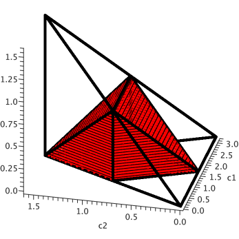
Figure 1: (Colour online) The Weyl chamber in $c_{1}c_{2}c_{3}$-space. The perfect entanglers make up the region highlighted in red.

Now that we have defined the coordinates and determined their ranges of values, we can choose an orientation; in this paper, we take the one such that the ordering

$$x = \left(x^{1},\ldots,x^{15}\right)$$

$$= \left(\vec{\alpha}_{1},\vec{\beta}_{1},\vec{\alpha}_{2},\vec{\beta}_{2},\vec{c}\right)$$

$$= \left(\alpha_{1},\theta_{1},\phi_{1},\beta_{1},\lambda_{1},\xi_{1},\alpha_{2},\theta_{2},\phi_{2},\beta_{2},\lambda_{2},\xi_{2},c_{1},c_{2},c_{3}\right)$$

forms a right-handed coordinate system.

We now want to find a Haar measure for $SU(4)$ in terms of these fifteen parameters. The basic method for finding such a measure for an $N$-dimensional simple compact Lie group $G$ is reviewed in the appendices, and the first step is to compute the Maurer-Cartan form $\Theta$ and write it in terms of the $N$ Hermitian Lie algebra generators $\{T_{A}\}$ and $N$ coordinate 1-forms $\{\mathrm{d}x^{\mu}\}$ as

$$\Theta = -iE^{A}{}_{\mu}(x)T_{A}\mathrm{d}x^{\mu}.$$

$E$ is therefore a real $N\times N$ matrix whose determinant gives us our invariant measure (up to an overall factor):

$$\mathrm{d}\mu \propto \left|\det E(x)\right|\mathrm{d}^{N}x,$$

where $\mathrm{d}^{N}x=\mathrm{d}x^{1}\wedge\ldots\wedge\mathrm{d}x^{N}$. Two of the ways of motivating this particular form of the measure are covered in the appendices, but both require us to somehow compute the determinant of $E$, which for $SU(4)$ is a $15\times 15$ matrix.

3 The Invariant Length Element and Haar Measure for $SU(4)$

In this section, we derive expressions for the invariant length element $\mathrm{d}s^{2}$ and the Haar measure $\mathrm{d}\mu$ for $SU(4)$. Both of these have been found before not just for $SU(4)$, but for $SU(n)$ and, indeed, for a great variety of simple compact Lie groups (see, for example [5, 6, 7] and references therein). However, the novelty of our approach is that these quantities will be in forms that are particularly suited for the description of two-qubit gates, namely, in the coordinate system defined in the previous section, which separates the purely local gates in $SU(2)\otimes SU(2)$ from the entangling gates in $\mathcal{A}$.

3.1 The Length Element

We choose to do the computation by first finding an invariant length element $\mathrm{d}s^{2}$ for $SU(4)$; since this will give the metric tensor via $\mathrm{d}s^{2}=g_{\mu\nu}(x)\mathrm{d}x^{\mu}\otimes\mathrm{d}x^{\nu}$, we may then use the relation $|\det E|\propto\sqrt{|\det g|}$. We could also have explicitly found the full $15\times 15$ matrix $E^{A}{}_{\mu}$ and then computed its determinant; this can be done using methods similar to those in [6, 7]. However, we found that the computation was somewhat simpler using $g_{\mu\nu}$ instead; we now describe the calculation that leads to this.

First, define the three $1$-forms $\Theta_{1,2,\mathcal{A}}$ by

$$\Theta_{1} = k_{1}^{-1}\mathrm{d}k_{1},$$

$$\Theta_{2} = \mathrm{d}k_{2}\,k_{2}^{-1},$$

$$\Theta_{\mathcal{A}} = A^{-1}\mathrm{d}A=\mathrm{d}A\,A^{-1}$$

(the latter holding because $\mathcal{A}$ is Abelian). It is straightforward to show that the $SU(4)$ Maurer-Cartan form $\Theta$ can be written as

$$\Theta = k_{2}^{-1}\left(A^{-1}\Theta_{1}A+\Theta_{\mathcal{A}}+\Theta_{2}\right)k_{2}$$

and that the invariant length, given (see Appendix B) by

$$\mathrm{d}s^{2} = -\mathrm{tr}\left(\Theta\dot{\otimes}\Theta\right),$$

can be expressed as

$$\mathrm{d}s^{2} = -\mathrm{tr}\left(\Theta_{1}\dot{\otimes}\Theta_{1}\right)-\mathrm{tr}\left(\Theta_{2}\dot{\otimes}\Theta_{2}\right)-\mathrm{tr}\left(\Theta_{\mathcal{A}}\dot{\otimes}\Theta_{\mathcal{A}}\right)$$ (3.1)

$$-\mathrm{tr}\left(\Theta_{1}\dot{\otimes}\Theta_{\mathcal{A}}+\Theta_{\mathcal{A}}\dot{\otimes}\Theta_{1}\right)-\mathrm{tr}\left(\Theta_{2}\dot{\otimes}\Theta_{\mathcal{A}}+\Theta_{\mathcal{A}}\dot{\otimes}\Theta_{2}\right)$$

$$-\mathrm{tr}\left(A^{-1}\Theta_{1}A\dot{\otimes}\Theta_{2}+\Theta_{2}\dot{\otimes}A^{-1}\Theta_{1}A\right).$$

The traces can be evaluated quickly if we choose an orthonormal basis for $SU(4)$; we take the fifteen generators $T_{0i}=(I\otimes\sigma_{i})/2$, $T_{i0}=(\sigma_{i}\otimes I)/2$ and $T_{ij}=(\sigma_{i}\otimes\sigma_{j})/2$, $i,j=x,y,z$, which satisfy

$$\mathrm{tr}\left(T_{A}T_{B}\right) = \delta_{AB}.$$

$SU(2)\otimes SU(2)$ is spanned by the six matrices $\{T_{0i},T_{i0}\}$ and $\mathcal{A}$ by the three matrices $\{T_{ii}\}$, so the matrices $k$ and $A$ are

$$k\left(\vec{\alpha},\vec{\beta}\right) = \exp\left[-i\sum_{j=1}^{3}\left(\alpha_{j}T_{0j}+\beta_{j}T_{j0}\right)\right],$$

$$A\left(\vec{c}\right) = \exp\left[-i\sum_{j=1}^{3}c_{j}T_{jj}\right].$$

Using these, we can explicitly compute $\Theta_{1}$, $\Theta_{2}$, $A$ and $\Theta_{\mathcal{A}}$, and thus the length element in (3.1). The first three terms give the invariant length elements of $SU(2)\otimes SU(2)$ (twice) and $\mathcal{A}$, and the next two terms vanish because the two subspaces are orthogonal to each other. The remaining term – the last – can be most conveniently written using what we know about $SU(2)$: the Maurer-Cartan form for this group has the form

$$\Theta_{SU(2)} = e^{i\vec{\alpha}\cdot\vec{\sigma}/2}\mathrm{d}e^{-i\vec{\alpha}\cdot\vec{\sigma}/2}$$

$$= -\frac{i}{2}\sum_{i}\zeta^{i}\left(\vec{\alpha}\right)\sigma_{i},$$

where the three 1-forms $\zeta^{x,y,z}$ are

$$\zeta^{x}\left(\vec{\alpha}\right) = \sin\theta\cos\phi\,\mathrm{d}\alpha+2\sin\left(\frac{\alpha}{2}\right)\left[\sin\left(\frac{\alpha}{2}\right)\sin\phi+\cos\left(\frac{\alpha}{2}\right)\cos\theta\cos\phi\right]\mathrm{d}\theta$$

$$+2\sin\left(\frac{\alpha}{2}\right)\sin\theta\left[\sin\left(\frac{\alpha}{2}\right)\cos\theta\cos\phi-\cos\left(\frac{\alpha}{2}\right)\sin\phi\right]\mathrm{d}\phi,$$

$$\zeta^{y}\left(\vec{\alpha}\right) = \sin\theta\sin\phi\,\mathrm{d}\alpha+2\sin\left(\frac{\alpha}{2}\right)\left[-\sin\left(\frac{\alpha}{2}\right)\cos\phi+\cos\left(\frac{\alpha}{2}\right)\cos\theta\sin\phi\right]\mathrm{d}\theta$$

$$+2\sin\left(\frac{\alpha}{2}\right)\sin\theta\left[\sin\left(\frac{\alpha}{2}\right)\cos\theta\sin\phi+\cos\left(\frac{\alpha}{2}\right)\cos\phi\right]\mathrm{d}\phi,$$

$$\zeta^{z}\left(\vec{\alpha}\right) = \cos\theta\,\mathrm{d}\alpha-2\sin\left(\frac{\alpha}{2}\right)\cos\left(\frac{\alpha}{2}\right)\sin\theta\,\mathrm{d}\theta-2\sin^{2}\left(\frac{\alpha}{2}\right)\sin^{2}\theta\,\mathrm{d}\phi.$$

The invariant length element for $SU(4)$ is therefore

$$\mathrm{d}s^{2} = \mathrm{d}s_{SU(2)}^{2}\left(\vec{\alpha}_{1}\right)+\mathrm{d}s_{SU(2)}^{2}\left(\vec{\beta}_{1}\right)+\mathrm{d}s_{SU(2)}^{2}\left(\vec{\alpha}_{2}\right)+\mathrm{d}s_{SU(2)}^{2}\left(\vec{\beta}_{2}\right)$$ (3.2)

$$+\mathrm{d}c_{1}\otimes\mathrm{d}c_{1}+\mathrm{d}c_{2}\otimes\mathrm{d}c_{2}+\mathrm{d}c_{3}\otimes\mathrm{d}c_{3}$$

$$-\left[\zeta^{x}\left(\vec{\alpha}_{1}\right)\otimes\zeta^{x}\left(-\vec{\alpha}_{2}\right)+\zeta^{x}\left(-\vec{\alpha}_{2}\right)\otimes\zeta^{x}\left(\vec{\alpha}_{1}\right)\right.$$

$$+\left.\zeta^{x}\left(\vec{\beta}_{1}\right)\otimes\zeta^{x}\left(-\vec{\beta}_{2}\right)+\zeta^{x}\left(-\vec{\beta}_{2}\right)\otimes\zeta^{x}\left(\vec{\beta}_{1}\right)\right]\cos c_{2}\cos c_{3}$$

$$-\left[\zeta^{y}\left(\vec{\alpha}_{1}\right)\otimes\zeta^{y}\left(-\vec{\alpha}_{2}\right)+\zeta^{y}\left(-\vec{\alpha}_{2}\right)\otimes\zeta^{y}\left(\vec{\alpha}_{1}\right)\right.$$

$$+\left.\zeta^{y}\left(\vec{\beta}_{1}\right)\otimes\zeta^{y}\left(-\vec{\beta}_{2}\right)+\zeta^{y}\left(-\vec{\beta}_{2}\right)\otimes\zeta^{y}\left(\vec{\beta}_{1}\right)\right]\cos c_{1}\cos c_{3}$$

$$-\left[\zeta^{z}\left(\vec{\alpha}_{1}\right)\otimes\zeta^{z}\left(-\vec{\alpha}_{2}\right)+\zeta^{z}\left(-\vec{\alpha}_{2}\right)\otimes\zeta^{z}\left(\vec{\alpha}_{1}\right)\right.$$

$$+\left.\zeta^{z}\left(\vec{\beta}_{1}\right)\otimes\zeta^{z}\left(-\vec{\beta}_{2}\right)+\zeta^{z}\left(-\vec{\beta}_{2}\right)\otimes\zeta^{z}\left(\vec{\beta}_{1}\right)\right]\cos c_{1}\cos c_{2}$$

$$-\left[\zeta^{x}\left(\vec{\alpha}_{1}\right)\otimes\zeta^{x}\left(-\vec{\beta}_{2}\right)+\zeta^{x}\left(-\vec{\beta}_{2}\right)\otimes\zeta^{x}\left(\vec{\alpha}_{1}\right)\right.$$

$$+\left.\zeta^{x}\left(\vec{\beta}_{1}\right)\otimes\zeta^{x}\left(-\vec{\alpha}_{2}\right)+\zeta^{x}\left(-\vec{\alpha}_{2}\right)\otimes\zeta^{x}\left(\vec{\beta}_{1}\right)\right]\sin c_{2}\sin c_{3}$$

$$-\left[\zeta^{y}\left(\vec{\alpha}_{1}\right)\otimes\zeta^{y}\left(-\vec{\beta}_{2}\right)+\zeta^{y}\left(-\vec{\beta}_{2}\right)\otimes\zeta^{y}\left(\vec{\alpha}_{1}\right)\right.$$

$$+\left.\zeta^{y}\left(\vec{\beta}_{1}\right)\otimes\zeta^{y}\left(-\vec{\alpha}_{2}\right)+\zeta^{y}\left(-\vec{\alpha}_{2}\right)\otimes\zeta^{y}\left(\vec{\beta}_{1}\right)\right]\sin c_{1}\sin c_{3}$$

$$-\left[\zeta^{z}\left(\vec{\alpha}_{1}\right)\otimes\zeta^{z}\left(-\vec{\beta}_{2}\right)+\zeta^{z}\left(-\vec{\beta}_{2}\right)\otimes\zeta^{z}\left(\vec{\alpha}_{1}\right)\right.$$

$$+\left.\zeta^{z}\left(\vec{\beta}_{1}\right)\otimes\zeta^{z}\left(-\vec{\alpha}_{2}\right)+\zeta^{z}\left(-\vec{\alpha}_{2}\right)\otimes\zeta^{z}\left(\vec{\beta}_{1}\right)\right]\sin c_{1}\sin c_{2},$$

where

$$\mathrm{d}s_{SU(2)}^{2}\left(\vec{\alpha}\right) = \mathrm{d}\alpha\otimes\mathrm{d}\alpha+4\sin^{2}\left(\frac{\alpha}{2}\right)\mathrm{d}\theta\otimes\mathrm{d}\theta+4\sin^{2}\left(\frac{\alpha}{2}\right)\sin^{2}\theta\,\mathrm{d}\phi\otimes\mathrm{d}\phi$$

is the $SU(2)$ invariant length element.

3.2 The Haar Measure

The metric tensor $g_{\mu\nu}$ can be extracted from (3.2), and, when considered as a $15\times 15$ matrix, has an associated determinant. A lengthy but straightforward calculation gives the result

$$\det g = \left[\vphantom{\sin^{2}\left(\frac{\beta_{2}}{2}\right)}\sin\left(c_{1}+c_{2}\right)\sin\left(c_{1}-c_{2}\right)\sin\left(c_{1}+c_{3}\right)\sin\left(c_{1}-c_{3}\right)\sin\left(c_{2}+c_{3}\right)\sin\left(c_{2}-c_{3}\right)\right.$$

$$\left.\times 256\sin^{2}\left(\frac{\alpha_{1}}{2}\right)\sin\theta_{1}\sin^{2}\left(\frac{\beta_{1}}{2}\right)\sin\lambda_{1}\sin^{2}\left(\frac{\alpha_{2}}{2}\right)\sin\theta_{2}\sin^{2}\left(\frac{\beta_{2}}{2}\right)\sin\lambda_{2}\right]^{2}.$$

Since $\left|\det E\right|\propto\sqrt{\left|\det g\right|}$, this allows us to determine, up to a proportionality constant, the Haar measure we want; to reflect the decomposition of $SU(4)$ into two copies of $SU(2)\otimes SU(2)$ and $\mathcal{A}=SU(4)/SU(2)\otimes SU(2)$, we write it as

$$\mathrm{d}\mu = \mathrm{d}\mu_{SU(2)}\left(\vec{\alpha}_{1}\right)\wedge\mathrm{d}\mu_{SU(2)}\left(\vec{\beta_{1}}\right)\wedge\mathrm{d}\mu_{SU(2)}\left(\vec{\alpha_{2}}\right)\wedge\mathrm{d}\mu_{SU(2)}\left(\vec{\beta_{2}}\right)$$

$$\wedge\mathrm{d}\mu_{\mathcal{A}}\left(c_{1},c_{2},c_{3}\right),$$

where $\mathrm{d}\mu_{SU(2)}$ is the normalised $SU(2)$ Haar measure in spherical coordinates

$$\mathrm{d}\mu_{SU(2)}(\alpha,\theta,\phi) = \frac{1}{8\pi^{2}}\sin^{2}\left(\frac{\alpha}{2}\right)\sin\theta\,\mathrm{d}\alpha\wedge\mathrm{d}\theta\wedge\mathrm{d}\phi$$

and $\mathrm{d}\mu_{\mathcal{A}}$ is the normalised Haar measure for the Abelian subgroup given by

$$\mathrm{d}\mu_{\mathcal{A}}\left(c_{1},c_{2},c_{3}\right) = \frac{48}{\pi}\left|\sin\left(c_{1}+c_{2}\right)\sin\left(c_{1}-c_{2}\right)\sin\left(c_{1}+c_{3}\right)\sin\left(c_{1}-c_{3}\right)\right.$$

$$\left.\times\sin\left(c_{2}+c_{3}\right)\sin\left(c_{2}-c_{3}\right)\right|\mathrm{d}c_{1}\wedge\mathrm{d}c_{2}\wedge\mathrm{d}c_{3}.$$

(Conveniently, the quantity in the absolute value above is manifestly nonnegative when $(c_{1},c_{2},c_{3})$ lies in the Weyl chamber, so taking the absolute value is redundant and we drop it from now on.) It is straightforward to confirm that these measures both integrate to unity over $SU(2)$ and $\mathcal{A}$ respectively. The normalised Haar measure on $SU(4)$ is therefore the wedge product of the five measures given:

$$\mathrm{d}\mu = \frac{3}{256\pi^{9}}\prod_{i=1}^{2}\left[\sin^{2}\left(\frac{\alpha_{i}}{2}\right)\sin\theta_{i}\sin^{2}\left(\frac{\beta_{i}}{2}\right)\sin\lambda_{i}\right]$$

$$\times\prod_{1\leq j<k\leq 3}\left[\sin\left(c_{j}+c_{k}\right)\sin\left(c_{j}-c_{k}\right)\right]\,\mathrm{d}^{15}x.$$

Two elements $U$ and $U^{\prime}$ of $SU(4)$ are locally equivalent to one another if one can be obtained from the other via either left or right multiplication by an element of $SU(2)\otimes SU(2)$. In other words, when $U$ and $U^{\prime}$ are decomposed into the form given in (2.1), they have the same matrix $A$. Thus, any local equivalence class $[U]\in\mathcal{A}$ is uniquely determined by coordinates $(c_{1},c_{2},c_{3})$ in the Weyl chamber, and so the invariant measure for the space of these classes is obtained by integrating over all the $SU(2)$ parameters. The result is the normalised Haar measure on $\mathcal{A}$:

$$\mathrm{d}\mu_{\mathcal{A}} = M_{\mathcal{A}}\left(c_{1},c_{2},c_{3}\right)\mathrm{d}c_{1}\wedge\mathrm{d}c_{2}\wedge\mathrm{d}c_{3},$$

where

$$M_{\mathcal{A}}\left(c_{1},c_{2},c_{3}\right) = \frac{48}{\pi}\left[\prod_{1\leq j<k\leq 3}\sin\left(c_{j}+c_{k}\right)\sin\left(c_{j}-c_{k}\right)\right].$$

Alternatively, using some trigonometric identities and a bit of algebra, we may rewrite this in a form somewhat more useful for computations:

$$M_{\mathcal{A}}\left(c_{1},c_{2},c_{3}\right) = \frac{3}{\pi}\left[\cos\left(2c_{1}\right)\cos\left(4c_{2}\right)+\cos\left(2c_{2}\right)\cos\left(4c_{3}\right)\right.$$ (3.3)

$$+\cos\left(2c_{3}\right)\cos\left(4c_{1}\right)-\cos\left(4c_{1}\right)\cos\left(2c_{2}\right)$$

$$\left.-\cos\left(4c_{2}\right)\cos\left(2c_{3}\right)-\cos\left(4c_{3}\right)\cos\left(2c_{1}\right)\right].$$

As this measure involves only elementary functions, computing the invariant volume of a region in $\mathcal{A}$ can often be done exactly, as we will show in Sections 4 and 5.

3.3 Local Invariants

We have just derived expressions for the measure and metric in terms of the three parameters $c_{1}$, $c_{2}$ and $c_{3}$; although both these expressions are (relatively) simple in form, they are only useful if we actually have values for these three coordinates. In practice, however, extracting $c_{1}$, $c_{2}$ and $c_{3}$ from an arbitrary $SU(4)$ matrix $U$ may be difficult. Fortunately, there are three far easier to obtain alternative parameters that can be used as coordinates on $\mathcal{A}$.

If we change from the standard computational basis $\{\left|00\right\rangle,\left|01\right\rangle,\left|10\right\rangle,\left|11\right\rangle\}$ to the Bell basis

$$\left\{\frac{1}{\sqrt{2}}\left(\left|00\right\rangle-i\left|11\right\rangle\right),-\frac{i}{\sqrt{2}}\left(\left|01\right\rangle+\left|10\right\rangle\right),\frac{1}{\sqrt{2}}\left(\left|01\right\rangle-\left|10\right\rangle\right),\frac{1}{\sqrt{2}}\left(\left|00\right\rangle+i\left|11\right\rangle\right)\right\},$$

then our $SU(4)$ matrices become $U_{\mathrm{B}}=Q^{\dagger}UQ=Q^{\dagger}k_{1}Ak_{2}Q$, where

$$Q = \frac{1}{\sqrt{2}}\left(\begin{array}[]{cccc}1&0&0&i\\ 0&i&1&0\\ 0&i&-1&0\\ 1&0&0&-i\end{array}\right).$$

The eigenvalues of the matrix $m=U_{\mathrm{B}}^{\mathrm{T}}U_{\mathrm{B}}$ determine all the local invariants of $U$, also called the Makhlin invariants [3]. The characteristic equation of $m$ is

$$\lambda^{4}-\mathrm{tr}(m)\lambda^{3}+\frac{1}{2}\left[\mathrm{tr}^{2}(m)-\mathrm{tr}\left(m^{2}\right)\right]\lambda^{2}-\mathrm{tr}^{*}(m)\lambda+1 = 0$$

and so $\mathrm{tr}(m)$ and $\mathrm{tr}(m^{2})$ give local invariants. These are complex numbers, so instead we may take as local invariants the three real numbers

$$g_{1}=\mathrm{Re}\left\{\frac{\mathrm{tr}^{2}(m)}{16}\right\},\,g_{2}=\mathrm{Im}\left\{\frac{\mathrm{tr}^{2}(m)}{16}\right\},\,g_{3}=\frac{\mathrm{tr}^{2}(m)-\mathrm{tr}\left(m^{2}\right)}{4}.$$ (3.5)

$m$, $m^{2}$ and their traces are readily computable using the simplest of matrix operations, and so values for $g_{1}$, $g_{2}$ and $g_{3}$ can be easily obtained for any $U\in SU(4)$.

Since these are local invariants, they must be functions only of $c_{1}$, $c_{2}$ and $c_{3}$; some computation shows that they are, and have the explicit forms

$$g_{1} = \frac{1}{4}\left[\cos\left(2c_{1}\right)+\cos\left(2c_{2}\right)+\cos\left(2c_{3}\right)+\cos\left(2c_{1}\right)\cos\left(2c_{2}\right)\cos\left(2c_{3}\right)\right],$$

$$g_{2} = \frac{1}{4}\sin\left(2c_{1}\right)\sin\left(2c_{2}\right)\sin\left(2c_{3}\right),$$

$$g_{3} = \cos\left(2c_{1}\right)+\cos\left(2c_{2}\right)+\cos\left(2c_{3}\right).$$ (3.6)

These can be used to embed the Weyl chamber into $g_{1}g_{2}g_{3}$-space. However, the Weyl chamber is no longer a simple tetrahedron in these coordinates, but rather an elongated “Eye of Sauron” shape [13, 14], as shown in Figure 2.

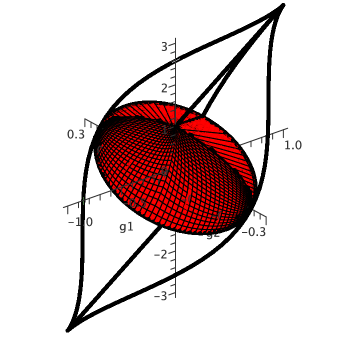
Figure 2: (Colour online) The Weyl chamber in $g_{1}g_{2}g_{3}$-space, with the region of perfect entanglers highlighted in red.

These functions are bijective when $c_{1}$, $c_{2}$ and $c_{3}$ lie within the Weyl chamber and we use the following inverse map $(g_{1},g_{2},g_{3})\mapsto(c_{1},c_{2},c_{3})$: first, find $z_{1}$, $z_{2}$ and $z_{3}$, the roots of the cubic equation

$$z^{3}-g_{3}z^{2}+\left(4\sqrt{g_{1}^{2}+g_{2}^{2}}-1\right)z+\left(g_{3}-4g_{1}\right) = 0,$$ (3.7)

ordered so that $z_{1}\leq z_{2}\leq z_{3}$. Then $c_{2}=\cos^{-1}(z_{2})/2$, $c_{3}=\cos^{-1}(z_{3})/2$ and $c_{1}$ is given by either $\cos^{-1}(z_{1})/2$ if $g_{2}\geq 0$ or $\pi-\cos^{-1}(z_{1})/2$ if $g_{2}<0$. (As used here, $\cos^{-1}$ is the principal value of the arccosine function, lying between $0$ and $\pi$.)

The Haar measure in terms of the local invariants has the relatively simple form

$$\mathrm{d}\mu_{\mathcal{A}}\left(g_{1},g_{2},g_{3}\right) = \frac{3}{\pi}\frac{\mathrm{d}g_{1}\wedge\mathrm{d}g_{2}\wedge\mathrm{d}g_{3}}{\sqrt{g_{1}^{2}+g_{2}^{2}}}.$$ (3.8)

However, the form of the length element is much more complicated in $g_{1}$, $g_{2}$ and $g_{3}$ than it is in $c_{1}$, $c_{2}$ and $c_{3}$: the Jacobian matrix $J$, which gives the coordinate transformation between $\vec{c}^{\mathrm{T}}=(c_{1},c_{2},c_{3})$ and $\vec{g}^{\mathrm{T}}=(g_{1},g_{2},g_{3})$, is defined by $\mathrm{d}\vec{g}=J\cdot\mathrm{d}\vec{c}$ and has the entries

$$J_{1i}=-\frac{1}{2}\left[1+\cos\left(2c_{j}\right)\cos\left(2c_{k}\right)\right]\sin\left(2c_{i}\right), j,k\neq i,\,j<k,$$

$$J_{2i}=\frac{1}{2}\cos\left(2c_{i}\right)\sin\left(2c_{j}\right)\sin\left(2c_{k}\right), j,k\neq i,\,j<k,$$

$$J_{3i}=-2\sin\left(2c_{i}\right).$$

The Euclidean length element $\mathrm{d}c_{1}^{2}+\mathrm{d}c_{2}^{2}+\mathrm{d}c_{3}^{2}$ therefore becomes $\mathrm{d}\vec{g}^{\mathrm{T}}\cdot(JJ^{\mathrm{T}})^{-1}\cdot\mathrm{d}\vec{g}$, and this can be written purely in terms of the local invariants:

$$JJ^{\mathrm{T}} = 2\left(\begin{array}[]{ccc}\rho-4g_{1}^{2}+2g_{2}^{2}+g_{1}g_{3}&g_{2}g_{3}-6g_{1}g_{2}&6\rho-2g_{1}g_{3}\\ g_{2}g_{3}-6g_{1}g_{2}&\rho+2g_{1}^{2}-4g_{2}^{2}-g_{1}g_{3}&-2g_{2}g_{3}\\ 6\rho-2g_{1}g_{3}&-2g_{2}g_{3}&16\rho+2-2g_{3}^{2}\end{array}\right),$$

where $\rho:=\sqrt{g_{1}^{2}+g_{2}^{2}}$. Inverting this matrix is possible but not particularly illuminating, so we do not do it here. However, it illustrates the key feature, that this part of $\mathrm{d}s^{2}$ can be written explicitly in terms of the local invariants without needing to solve (3.7).

Unfortunately, the cross-terms in (3.2) – those involving the $\zeta$-forms – depend on the local invariants through $\sin c_{i}\sin c_{j}$ and $\cos c_{i}\cos c_{j}$, and writing these explicitly in terms of $g_{1}$, $g_{2}$ and $g_{3}$ leads to an extremely complicated form for the length element. Although this part of $\mathrm{d}s^{2}$ will not figure into any calculation at a fixed point in $SU(2)\otimes SU(2)$, if one is to compute the invariant distance between two arbitrary points in $SU(4)$, it is this form that must be used if we choose the local invariants as coordinates.

3.4 Extension to $U(4)$

We have so far discussed only the two-qubit gates that lie in $SU(4)$ and we will continue to concentrate on this group for the remainder of this article; however, as stated in the introduction, a general two-qubit gate will be an element of $U(4)$, so we digress momentarily to explain how all of the results just obtained may be easily extended to all of $U(4)$.

This is done through the decomposition $U(4)=[0,\pi/2)\times SU(4)$, where the first term in the Cartesian product contributes to an overall phase factor:

$$U = e^{i\chi}k_{1}Ak_{2},$$

with $k_{1}$, $k_{2}$ and $A$ as before and $\chi\in[0,\pi/2)$ (considered as a group with addition modulo $\pi/2$). The invariant length element and Haar measure of $U(4)$ are therefore obtained from those of $SU(4)$ via, respectively, the addition of $4\mathrm{d}\chi\otimes\mathrm{d}\chi$ to (3.2) and the wedge product of $2\mathrm{d}\chi/\pi$ with (3.2).

However, the coordinates $g_{1}$, $g_{2}$ and $g_{3}$ as given in (3.5) will depend on $\chi$, and so must be redefined so as to be independent of not only the $SU(2)\otimes SU(2)$ local gates, but also the $U(1)$ phase. Luckily, this is accomplished by simple division by the determinant of $U$ [2]:

$$g_{1}=\mathrm{Re}\left\{\frac{\mathrm{tr}^{2}(m)}{16\det U}\right\},\,g_{2}=\mathrm{Im}\left\{\frac{\mathrm{tr}^{2}(m)}{16\det U}\right\},\,g_{3}=\frac{\mathrm{tr}^{2}(m)-\mathrm{tr}\left(m^{2}\right)}{4\det U}.$$

This modification ensures that the coordinate transformation from $(c_{1},c_{2},c_{3})$ to $(g_{1},g_{2},g_{3})$ given by (3.6) remains the same. Thus, all our results for $SU(4)$ will easily extend to $U(4)$; however, for the remainder of this article, we shall once again concern ourselves only with $SU(4)$.

4 Perfect Entanglers

The elements of $SU(4)$ that perfectly entangle two-qubit states all lie within the subset of the Weyl chamber bounded by the planes $c_{1}+c_{2}=\pi/2$, $c_{1}-c_{2}=\pi/2$ and $c_{2}+c_{3}=\pi/2$. This region is the interior of the 7-faced polyhedron with vertices at $(\pi/2,0,0)$, $(\pi/4,\pi/4,0)$, $(3\pi/4,\pi/4,0)$, $(\pi/2,\pi/2,0)$, $(\pi/4,\pi/4,\pi/4)$ and $(3\pi/4,\pi/4,\pi/4)$, the red volume illustrated in Figure 1.

At any specific point in the $SU(2)\otimes SU(2)$ orbit, this region fills exactly half of the Weyl chamber: if both $k_{1}$ and $k_{2}$ are constant, then $\mathrm{d}s^{2}=\mathrm{d}c_{1}^{2}+\mathrm{d}c_{2}^{2}+\mathrm{d}c_{3}^{2}$, and the space is flat. The Euclidean volume – calculated with the normalised measure $\frac{24}{\pi^{3}}\,\mathrm{d}c_{1}\wedge\mathrm{d}c_{2}\wedge\mathrm{d}c_{3}$ – is $1/2$.

However, if we are more concerned with those $SU(4)$ elements that entangle the two qubits, we are not concerned with what the volume of the entangling chamber is at a specific point in $SU(2)\otimes SU(2)$; in fact, since this subgroup only consists of local gates, we are not interested at all in the values of $k_{1}$ and $k_{2}$, but rather only in those values of $A$ where $(c_{1},c_{2},c_{3})$ is in the perfectly-entangling chamber.

Therefore, the total volume in $SU(4)$ occupied by the space of perfect entanglers is obtained by integrating the Haar measure around the full $SU(2)\otimes SU(2)$ orbit, i.e., all values of $(\vec{\alpha}_{1},\vec{\beta}_{1},\vec{\alpha}_{2},\vec{\beta}_{2})$, as well as the values of $c_{1}$, $c_{2}$ and $c_{3}$ giving the perfect entanglers. Since the four $SU(2)$ measures are already normalised, and $M_{\mathcal{A}}(c_{1},c_{2},c_{3})$ is symmetric around $c_{1}=\pi/2$, the integral over the subset of perfect entanglers is

$$V_{\mathrm{PE}} = 2\int_{\pi/4}^{\pi/2}\mathrm{d}c_{1}\left[\int_{\pi/2-c_{1}}^{\pi/4}\mathrm{d}c_{2}\int_{0}^{c_{2}}\mathrm{d}c_{3}+\int_{\pi/4}^{c_{1}}\mathrm{d}c_{2}\int_{0}^{\pi/2-c_{2}}\mathrm{d}c_{3}\right]M_{\mathcal{A}}\left(c_{1},c_{2},c_{3}\right)$$

$$= \frac{8}{3\pi},$$

so we obtain the rather surprising result that the perfect entanglers occupy over $84\%$ of $SU(4)$!

There are two important remarks to make concerning this result: first, we chose to do the computation in $c_{1}c_{2}c_{3}$-space because, in these coordinates, the Haar measure has a relatively simple form and the boundary of the region of perfect entanglers is bounded by planes, making the integral of $\mathrm{d}\mu$ very straightforward. We could also have chosen to do the integral in $g_{1}g_{2}g_{3}$-space using (3.8), but the region of perfect entanglers – the red “pupil” in Figure 2 – has boundaries much more complicated than planes, and so the volume integral would be much more difficult to calculate. However, the invariance of our measure ensures that we would obtain the same result of $8/3\pi$ if we did use the Makhlin invariants.

Secondly, we have shown that perfect entanglers make up a majority of all two-qubit gates. From the point of view of quantum information processing, this is good news, because it suggests that it may be easier than expected to create a perfectly-entangling gate. In fact, if we are able to pick a two-qubit gate purely at random, we would get a perfect entangler nearly 85% of the time!

It is this second point that we will address in more detail in the next section: the computation of the invariant volumes of specific regions in $SU(4)$, those surrounding the types of gates of particular interest to quantum computing, e.g., the CNOT and SWAP gates.

Note added in proof: During the refereeing process following the submission of this manuscript, we became aware of [15], in which two of our results – the form of the Haar measure on $\mathcal{A}$ and the volume of the space of perfect entanglers – were independently obtained. However, the technique used in the aforementioned article differs greatly from ours: the measure was obtained by using results from the theory of random matrices [16], which gives only its form on $\mathcal{A}$ and not on the entirety of $SU(4)$. In contrast, our approach is geometrically motivated and gives much more general results: we obtain the measure on $\mathcal{A}$ by first constructing an invariant length element for $SU(4)$ and then using the associated metric to find a Haar measure for the entire group. The measure on $\mathcal{A}$ follows from integration around the orbit of $SU(2)\otimes SU(2)$. However, in both cases, once a measure on $\mathcal{A}$ is obtained, the computation of the volume of the space of perfect entanglers readily follows.

5 Uses in Quantum Control

The implementation of any two-qubit quantum computer requires, of course, quantum gates that operate on the two qubits. Creating such gates presents a formidable technical challenge; one must devise a system in which an element of $SU(4)$ can evolve from an initial state (most usually the identity element, but in principle any $SU(4)$ matrix) to a final state that is the desired gate.

In practice, however, we cannot create a gate exactly. We can only end up within a certain neighbourhood of a given gate. For example, an arbitrary element of $SU(4)$ depends on fifteen parameters $x^{1},\ldots,x^{15}$; if the gate we want is located at the exact point $(x^{*1},\ldots,x^{*15})$, we will only ever be able to evolve to a matrix within a certain parameter range around this point, for example, a cubic region $(x^{*1}\pm\Delta x^{1},\ldots,x^{*15}\pm\Delta x^{15})$.

The likelihood of us being able to evolve the gate into this region depends on its size: the greater the volume of the region, the bigger a target it presents for us to shoot at. Certain gates may be easier to implement with greater precision if the target volume over a given parameter range is large; if it is small, then it may be quite difficult to end up inside the volume, and we may have to increase the parameter range (and thus lose precision) in order to finish near the desired gate.

So how do we determine the target sizes? If $SU(4)$ were a flat space, then all target sizes would be the same for a given parameter range; for example, the cubic region described above would have volume $2^{15}\Delta x^{1}\ldots\Delta x^{15}$ regardless of what $(x^{*1},\ldots,x^{*15})$ was. But we know that $SU(4)$ has a non-Euclidean metric, and is not flat. Therefore, the volume of a region – obtained by integration of the Haar measure – can depend on both the location of the final gate and the range of parameters describing its neighbourhood. The resulting volumes will tell us how large a target the selected gates present for the range of parameters we choose, and can therefore be used as an indication of how difficult a gate is to achieve with precision.

5.1 Volumes of Target Cubes

As above, we are only concerned with gates that are equivalent up to local $SU(2)\otimes SU(2)$ operations, so any target volume we compute will include an integration over all of this subgroup. Thus, we will only have to compute integrals over regions of $\mathcal{A}$, since all points in this Abelian group are indeed distinct modulo local single-qubit operations. So if $[U]$ is the equivalence class of the gate $U$, and $\mathcal{U}$ is a neighbourhood of $[U]$ in $\mathcal{A}$, the volume in $SU(4)$ that this region occupies is

$$V(\mathcal{U}) = \int_{\left(SU(2)\otimes SU(2)\right)\times\left(SU(2)\otimes SU(2)\right)\times\mathcal{U}}\mathrm{d}\mu$$

$$= \int_{\mathcal{U}}\mathrm{d}\mu_{\mathcal{A}}.$$

The nonzero curvature of $SU(4)$ makes it likely that regions in $\mathcal{A}$ that are described by the same range of coordinates might not have the same volumes. Specifically, if we choose $(c_{1},c_{2},c_{3})$ as our coordinates in $\mathcal{A}$, a cube of side length $a$ centred at a point $(c_{1}^{*},c_{2}^{*},c_{3}^{*})$ in the Weyl chamber will not only have a volume different from $a^{3}$, but this volume will also vary depending on where it is centred.

The following results illustrate these properties. In all cases, the region integrated over is a cube of side length $a$ centred on the five basic gates discussed in [4] (plus two others, for illustrative purposes) and whose sides are parallel to the $c_{1}$, $c_{2}$ and $c_{3}$ axes:

1. $[\mathbb{1}]$ at $(0,0,0)$, with $0\leq a\leq\pi$:

   $$V = \frac{3}{2\pi}\left[8a+a\cos(3a)-9a\cos(a)-3\sin(3a)+12\sin(2a)-15\sin(a)\right].$$

   For small $a$, this is $a^{9}/40\pi+O(a^{11})$.

2. $[\mathrm{SWAP}]$ at $(\pi/2,\pi/2,\pi/2)$, with $0\leq a\leq\pi$:

   $$V = \frac{3}{2\pi}\left[8a+a\cos(3a)-9a\cos(a)-3\sin(3a)+12\sin(2a)-15\sin(a)\right].$$

   For small $a$, this is $a^{9}/40\pi+O(a^{11})$.

3. $[\sqrt{\mathrm{SWAP}}]$ at $(\pi/4,\pi/4,\pi/4)$, with $0\leq a\leq\pi/2$:

   $$V = \frac{3}{2\pi}\left[2a\sin(3a)+6a\sin(a)+3\cos(3a)-3\cos(a)\right].$$

   For small $a$, this is $8a^{6}/5\pi+O(a^{8})$.

4. $[\mbox{B-gate}]$ at $(\pi/2,\pi/4,0)$, with $0\leq a\leq\pi/4$:

   $$V = \frac{3a}{\pi}\left[\cos(a)-\cos(3a)\right].$$

   For small $a$, this is $12a^{3}/\pi+O(a^{5})$.

5. $[\mathrm{CNOT}]$/$[\mathrm{CPHASE}]$ at $(\pi/2,0,0)$, with $0\leq a\leq\pi/2$:

   $$V = \frac{1}{2\pi}\left[8a+7a\cos(3a)-15a\cos(a)-9\sin(3a)+12\sin(2a)+3\sin(a)\right].$$

   For small $a$, this is $4a^{5}/\pi+O(a^{7})$.

6. $[\mathrm{DCNOT}]$ at $(\pi/2,\pi/2,0)$, with $0\leq a\leq\pi/2$:

   $$V = \frac{1}{2\pi}\left[8a+7a\cos(3a)-15a\cos(a)-9\sin(3a)+12\sin(2a)+3\sin(a)\right].$$

   For small $a$, this is $4a^{5}/\pi+O(a^{7})$.

7. Gate at $(\frac{\pi}{2},\frac{\pi}{4},\frac{\pi}{4})$, with $0\leq a\leq\pi/4$:

   $$V = \frac{1}{2\pi}\left[3\cos{(a)}-3\cos{(3a)}-4a\sin{(3a)}\right].$$

   For small $a$, this is $4a^{4}/\pi+O(a^{6})$.

(The upper bounds on the values of $a$ in the above expressions come from the fact that if the cubes are too big, then we cannot use equation (3.3), since it is valid only in the Weyl chamber. Computing the volumes of larger cubes is possible but difficult, and we do not do it here.)

The volumes for small values of $a$ are included to provide a means of comparison: the smaller the cube is, the closer we are to the exact gate $[U]$, and so if we are to implement this gate with any reasonable degree of precision, $a$ will have to be small. The leading-order term in the small-$a$ expansion therefore gives the approximate scaling behaviour for each volume, and we see that the largest volume occurs at the [B-gate] ($V\sim a^{3}$) and the smallest at the identity and [SWAP] gates ($V\sim a^{9}$), with the volumes of all other gates lying in between.

All controlled gates have equivalence classes that lie on the $c_{1}$-axis between the origin and $c_{1}=\pi/2$, and the invariant volume of a cube of side length $a$ around each of them can be computed in the same fashion as the fixed gates above: if the centre of the cube is at $(c_{1}^{*},0,0)$, then if $0\leq a\leq c_{1}^{*}$,

$$V\left(c_{1}^{*},0,0\right) = \frac{1}{2\pi}\left\{8a+a\cos(3a)-9a\cos(a)\right.$$

$$-\left[3a\cos(3a)-3a\cos(a)-3\sin(3a)+9\sin(a)\right]\cos\left(2c_{1}^{*}\right)$$

$$\left.+\left[3a\cos(3a)-3a\cos(a)-6\sin(3a)+12\sin(2a)-6\sin(a)\right]\cos\left(4c_{1}^{*}\right)\right\}$$

$$= \frac{a^{5}}{2\pi}\left\{3-4\cos\left(2c_{1}^{*}\right)+\cos\left(4c_{1}^{*}\right)-\frac{a^{2}}{15}\left[15-26\cos\left(2c_{1}^{*}\right)+11\cos\left(4c_{1}^{*}\right)\right]\right.$$

$$\left.+\frac{a^{4}}{5040}\left[819-1640\cos\left(2c_{1}^{*}\right)+905\cos\left(4c_{1}^{*}\right)\right]\right\}+O\left(a^{11}\right).$$

Thus, for any $c_{1}^{*}>0$, the invariant volume scales as $a^{5}$. (For $c_{1}^{*}=\pi/2$, we recover the previous result shared by the [CNOT] and [CPHASE] gates.)

All of the above gates lie somewhere on the boundary of the Weyl chamber; if we take a cube of side length $a$ that lies entirely within the Weyl chamber, then its volume as a function of its centre $(c_{1}^{*},c_{2}^{*},c_{3}^{*})$ is

$$V(c^{*}_{1},c^{*}_{2},c^{*}_{3}) = \frac{3a}{2\pi}\sin{(a)}\sin{(2a)}\left[\cos{(2c^{*}_{1})}\cos{(4c^{*}_{2})}-\cos{(4c^{*}_{1})}\cos{(2c^{*}_{2})}\right.$$

$$+\cos{(2c^{*}_{2})}\cos{(4c^{*}_{3})}-\cos{(4c^{*}_{2})}\cos{(2c^{*}_{3})}$$

$$\left.+\cos{(4c^{*}_{1})}\cos{(2c^{*}_{3})}-\cos{(2c^{*}_{1})}\cos{(4c^{*}_{3})}\right]$$

$$= \frac{1}{2}a\sin{(a)}\sin{(2a)}M_{\mathcal{A}}\left(c^{*}_{1},c^{*}_{2},c^{*}_{3}\right).$$

For small $a$, the prefactor is approximately $a^{3}$, the Euclidean volume of the cube, and so in this limit $V/a^{3}$ is $M_{\mathcal{A}}$, and thus tells us how much larger or smaller the actual invariant volume is than the Euclidean volume.

Figure 3 plots $M_{\mathcal{A}}$ for three horizontal slices of the Weyl chamber, at $c_{3}^{*}=\pi/12$, $\pi/6$ and $\pi/4$. These illustrate that $M_{\mathcal{A}}$ vanishes on the boundary of the chamber and peaks in the interior for all $c_{3}^{*}>0$. Furthermore, this maximum value increases as $c_{3}^{*}$ decreases toward zero. In fact, it is on this bottom face that $M_{\mathcal{A}}$ takes on its global maximum of $12/\pi$ at $c_{1}^{*}=\pi/2$ and $c_{2}^{*}=\pi/4$. This demonstrates that cubes near the [B-gate] present, for a given side length, the biggest targets.

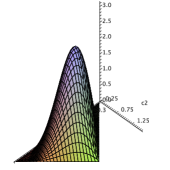
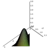
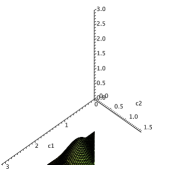
Figure 3: (Colour online) Cube volumes within the Weyl chamber. The volume factor $M_{\mathcal{A}}$ as a function of $(c_{1}^{*},c_{2}^{*})$ on horizontal slices with, from left to right, $c_{3}^{*}=\pi/12$, $c_{3}^{*}=\pi/6$ and $c_{3}^{*}=\pi/4$.

5.2 Makhlin Invariants and Target Cylinders

As is evident from Figure 2, the boundary of the Weyl chamber in $g_{1}g_{2}g_{3}$-space is no longer a collection of flat planes but a curved surface. Computing the volumes of regions that abut the boundary (precisely where many of the gates of interest are located) is therefore likely to be far more difficult than in $c_{1}c_{2}c_{3}$-space.

It is possible, however, to find exact expressions for the volumes of some regions that lie entirely within the Weyl chamber. This is most easily done by converting to cylindrical coordinates $(\rho,\phi,z)$ given by $g_{1}=\rho\cos\phi$, $g_{2}=\rho\sin\phi$ and $g_{3}=z$. The measure in these coordinates is very simple: $3\mathrm{d}\rho\wedge\mathrm{d}\phi\wedge\mathrm{d}z/\pi$. Using this, we can explicitly compute the volumes of various regions centred on the origin:

Cube of side length $$a V=\frac{12a^{2}}{\pi}\ln\left(\sqrt{2}+1\right).$$:

Cylinder of height $$h R V=6Rh.$$ and axial radius :

Sphere of radius $$R V=3\pi R^{2}.$$:

For regions not centred on the origin, the volumes of cubes and spheres tend to be more difficult to compute, but a closed-form expression can be found for the volume of a cylinder (with axis in $g_{3}$ direction) of height $h$ and radius $R$ centred at $(g_{1}^{*},g_{2}^{*},g_{3}^{*})$. If $g_{1}^{*}=g_{2}^{*}=0$, the volume is the same as at the origin, namely, $6Rh$. If either $g_{1}^{*}$ or $g_{2}^{*}$ is nonzero, then $\rho^{*}=\sqrt{(g_{1}^{*})^{2}+(g_{2}^{*})^{2}}$ is positive and the invariant volume of the cylinder is

$$V\left(g_{1}^{*},g_{2}^{*},g_{3}^{*}\right) = \left\{\begin{array}[]{crl}\frac{12Rh}{\pi}E\left(\frac{\rho^{*}}{R}\right)&\mbox{for}&R\geq\rho^{*},\\ \frac{12\rho^{*}h}{\pi}\left[E\left(\frac{R}{\rho^{*}}\right)+\left(\frac{R^{2}}{(\rho^{*})^{2}}-1\right)K\left(\frac{R}{\rho^{*}}\right)\right]&\mbox{for}&R<\rho^{*},\end{array}\right.$$

where $K(k)$ and $E(k)$ are the complete elliptic integrals of the first and second kind respectively:

$$K(k)=\int_{0}^{\pi/2}\frac{\mathrm{d}\phi}{\sqrt{1-k^{2}\sin^{2}\phi}}, E(k)=\int_{0}^{\pi/2}\mathrm{d}\phi\,\sqrt{1-k^{2}\sin^{2}\phi}.$$

For small cylinders with $R\ll\rho^{*}$, we find

$$V\left(g_{1}^{*},g_{2}^{*},g_{3}^{*}\right) \approx \frac{3R^{2}h}{\sqrt{\left(g_{1}^{*}\right)^{2}+\left(g_{2}^{*}\right)^{2}}},$$

so the volume of the cylinder decreases as we move away from the $g_{3}$-axis, entirely consistent with the result we obtained in $c_{1}c_{2}c_{3}$-space.

6 Conclusions

In order to study the geometric properties of $SU(4)$ in a way that is particularly suitable to a quantum information context – where the emphasis is on the entangling capabilities of two-qubit operations – we have utilised a parametrisation of $SU(4)$ that reflects the natural decomposition of two-qubit gates into local (single-qubit) $SU(2)\otimes SU(2)$ and purely nonlocal (two-qubit) $SU(4)/SU(2)\otimes SU(2)$ factors. The latter (denoted by $\mathcal{A}$) corresponds to the maximal Abelian subgroup of $SU(4)$ and is parametrised by three real coordinates.

In this parametrisation, we have calculated the invariant length element and the Haar measure of $SU(4)$, with the latter normalised to provide unit total volume of the group. These calculations also show that while the purely nonlocal part of the two-qubit operations is geometrically flat, the local part carries a curvature that is carried over to the curvature of $SU(4)$.

We continue with a discussion of the metric properties of the Abelian subgroup $\mathcal{A}$ of $SU(4)$ in the context of a different choice of coordinates, namely, the Makhlin invariants. Although these invariants are easily determined from a general element of $SU(4)$ and the Haar measure takes a relatively simple form, the invariant length element is far more complicated. Its form can be determined but is not particularly illuminating; however, the results we present are sufficient to allow one to compute the invariant distance between two arbitrary points should the local invariants be selected as the preferred coordinates for $\mathcal{A}$.

These results allow us to compute the invariant volume of any region in the Abelian subgroup $\mathcal{A}$ of $SU(4)$, i.e., any region in the space of local equivalence classes of two-qubit gates. We first apply it to the set of perfect entanglers; these gates, which are capable of creating maximally entangled states out of some product states, correspond to half of the local equivalence classes. We found that the invariant volume of perfect entanglers occupies more than $84\%$ of the total volume of two-qubit gates, which means that, in fact, the majority of the two-qubit gates are perfect entanglers. (Our form of the Haar measure on $\mathcal{A}$ and our volume of the space of perfect entanglers are in complete agreement with the recent independently-obtained results in [15].)

Next, we use the Haar measure to find the invariant volumes of locally-equivalent regions around specific gates. All these regions are described by the same range of parameters, but due to the curvature of the space, not all these regions have the same volume. In fact, the invariant volumes depend entirely on where in $\mathcal{A}$ the region lies. We find that the volume is smallest around the identity and SWAP gates and largest at the B-gate, with all other volumes falling in between.

These results are relevant to quantum information processing and its physical implementation in general, and in particular, to recent efforts [4] to use optimal control approach to generate two-qubit quantum operations, where the control objective is any gate of a given entangling power rather than a specific two-qubit gate. In cases where the objective is to achieve a perfect entangling gate, our conclusion that the majority of all gates are perfect entanglers is highly encouraging.

If the objective is to create one of the more familiar logical gates, our results show that generating a SWAP gate with any precision may be difficult due to the low density of gates in its neighbourhood, whereas the high density near the B-gate suggests that it could be relatively easy to generate. Since the B-gate is one of the gates that is needed to create a universal quantum computer, this is also an encouraging result.

Appendices

Appendix A Haar Measures on Compact Lie Groups

Suppose $G$ is a simple compact $N$-dimensional Lie group with corresponding Lie algebra $g$. Let $\{x^{\mu}|\mu=1,\ldots,N\}$ be a set of local coordinates on the manifold $M$ underlying $G$, with $\{\mathrm{d}x^{\mu}\}$ the associated $1$-forms. Given $U(x)\in G$, we may construct the Maurer-Cartan $1$-form $\Theta$ as

$$\Theta := U^{-1}\mathrm{d}U.$$

This $1$-form is left-invariant and right-covariant; in other words, under the left-translation

$$U(x) \mapsto VU(x),$$

$\Theta$ is unchanged, and under the right-translation

$$U(x) \mapsto U(x)W^{-1},$$

$\Theta$ transforms via conjugation by $W$: $\Theta\mapsto W\Theta W^{-1}$.

We want an invariant measure for $G$, namely, a positive-definite $N$-form on $M$ that does not change under either the left- or right-translations above, and thus may play the role of a volume element on the group. We construct it by noticing that the wedge product of $\Theta$ with itself any number of times is also left-invariant and right-covariant. Thus, if we have a finite-dimensional irreducible representation (irrep) $\rho$ of $g$, then taking the trace of $\Theta^{\wedge N}$ in this irrep returns an $N$-form that is left-invariant automatically and right-invariant due to the cyclicity of the trace:

$$\mathrm{tr}_{\rho}\left(\Theta^{\wedge N}\right) \mapsto \mathrm{tr}_{\rho}\left(W\Theta^{\wedge N}W^{-1}\right)$$

$$= \mathrm{tr}_{\rho}\left(\Theta^{\wedge N}\right).$$

Thus, this is an invariant measure for $G$. For compact Lie groups, any such measure is unique up to an overall multiplicative factor, and is called the Haar measure $\mathrm{d}\mu$ of the group.

Suppose $\{T_{A}|A=1,\ldots,N\}$ is a Hermitian basis for the simple compact Lie algebra $g$. Since $\Theta$ is a $1$-form that takes values in $g$, we may write it (using Einstein summation convention) both in terms of the $1$-forms $\mathrm{d}x^{1,\ldots,N}$ and the generators $T_{1,\ldots,N}$ as

$$\Theta = -iE^{A}{}_{\mu}\left(x\right)T_{A}\mathrm{d}x^{\mu},$$

where each of the $N^{2}$ components $E^{A}{}_{\mu}$ is simply a numerical function of the local coordinates. If we wedge $\Theta$ with itself $N$ times, then we obtain

$$\Theta^{\wedge N} = (-i)^{N}E^{A_{1}}{}_{\mu_{1}}\ldots E^{A_{N}}{}_{\mu_{N}}T_{A_{1}}\ldots T_{A_{N}}\mathrm{d}x^{\mu_{1}}\wedge\ldots\wedge\mathrm{d}x^{\mu_{N}}$$

$$= (-i)^{N}E^{A_{1}}{}_{\mu_{1}}\ldots E^{A_{N}}{}_{\mu_{N}}T_{A_{1}}\ldots T_{A_{N}}\epsilon^{\mu_{1}\ldots\mu_{N}}\mathrm{d}^{N}x,$$

where $\epsilon$ is the $N$-dimensional Levi-Civita symbol and $\mathrm{d}^{N}x$ is shorthand for $\mathrm{d}x^{1}\wedge\ldots\wedge\mathrm{d}x^{N}$. If we think of $E$ as an $N\times N$ matrix, then

$$\Theta^{\wedge N} = (-i)^{N}\det E\,\,T_{A_{1}}\ldots T_{A_{N}}\epsilon^{A_{1}\ldots A_{N}}\mathrm{d}^{N}x.$$

We therefore see that

$$\mathrm{tr}_{\rho}\left(\Theta^{\wedge N}\right) = (-i)^{N}\mathrm{tr}_{\rho}\left(T_{A_{1}}\ldots T_{A_{N}}\epsilon^{A_{1}\ldots A_{N}}\right)\det E\;\mathrm{d}^{N}x,$$

where $\rho$ is any irrep of $g$. The trace is just an overall multiplicative factor, and since the Haar measure is determined only up to proportionality, we conclude that

$$\mathrm{d}\mu \propto \left|\det E(x)\right|\mathrm{d}^{N}x.$$

Taking the absolute value of the determinant ensures that the measure is positive-definite if the proportionality constant is positive. Because $G$ is compact, the integral of this $N$-form over the underlying manifold $M$ is finite, and so we can fix the constant of proportionality such that this integral is unity. This defines the normalised Haar measure for a compact simple Lie group:

$$\mathrm{d}\mu = \frac{\left|\det E(x)\right|\mathrm{d}^{N}x}{\int_{M}\left|\det E\left(x^{\prime}\right)\right|\mathrm{d}^{N}x^{\prime}}.$$

An important point: for an arbitrary Lie group $G$, it is possible that the trace over the generators or the determinant of $E$ could vanish. However, both are nonzero if $G$ is simple, which we have assumed. But this general method may be extended to nonsimple compact Lie groups as well: if $G=G_{1}\times G_{2}\times\ldots\times G_{M}$ where each $G_{i}$ is compact and simple, then the product of their normalised Haar measures

$$\mathrm{d}\mu = \mathrm{d}\mu_{G_{1}}\wedge\mathrm{d}\mu_{G_{2}}\wedge\ldots\wedge\mathrm{d}\mu_{G_{M}}$$

is a positive-definite left- and right-invariant $N$-form, and thus a normalised Haar measure on $G$.

As an example, consider $U(n)$: this is a nonsimple compact Lie group that is equal to $[0,2\pi/n)\times SU(n)$, where $[0,2\pi/n)$ is considered as a group under addition modulo $2\pi/n$. Any element of $U(n)$ has the form $e^{i\chi}U$, with $\chi\in[0,2\pi/n)$ and $U\in SU(n)$. Then if $\mathrm{d}\mu_{SU(n)}$ is the normalised Haar measure for $SU(n)$, then

$$\mathrm{d}\mu = \frac{n\mathrm{d}\chi}{2\pi}\wedge\mathrm{d}\mu_{SU(n)}$$

is the normalised Haar measure for $U(n)$.

Appendix B Metric Structures of Simple Lie Groups

Another standard way of obtaining the invariant measure for a compact Lie group is via the natural metric structure of the underlying manifold that is induced by the Maurer-Cartan form. By “metric structure”, we mean a way of measuring lengths and distances in the Lie group: if $x$ and $y$ are the coordinates of the two elements $U(x)$ and $U(y)$ in $G$, then we want a function $s(x,y)$ that tells us “how far” $U(x)$ and $U(y)$ are from each other.

Since finite lengths can be built up from infinitesimal lengths, we need a quantity $\mathrm{d}s$ so that the length of a path $\Gamma$ connecting two points is $\int_{\Gamma}\mathrm{d}s$; this is given by a two-form written in terms of a symmetric metric tensor $g_{\mu\nu}$ via

$$\mathrm{d}s^{2} = g_{\mu\nu}(x)\mathrm{d}x^{\mu}\otimes\mathrm{d}x^{\nu}.$$

However, we want this length element to be invariant under the action $U(x)\mapsto VU(x)W^{-1}$, since this gives the coordinate transformations on $G$. The Maurer-Cartan form gives us everything we need to define such an element: define the $N$ Lie algebra-valued functions $\Theta_{1},\ldots,\Theta_{N}$ as the coefficients of the coordinate 1-forms, namely,

$$\Theta = \Theta_{\mu}(x)\mathrm{d}x^{\mu}=\left[-iE^{A}{}_{\mu}(x)T_{A}\right]\mathrm{d}x^{\mu}.$$

If we both left- and right-act on $U(x)$ via $VU(x)W^{-1}$, we know that $\Theta\mapsto W\Theta W^{-1}$; group multiplication only affects the Lie algebra-valued part of $\Theta$, so

$$\Theta_{\mu} \mapsto W\Theta_{\mu}W^{-1}.$$

Therefore,

$$\Theta_{\mu}\Theta_{\nu} \mapsto W\left(\Theta_{\mu}\Theta_{\nu}\right)W^{-1}.$$

This is neither invariant nor symmetric in $\mu$ and $\nu$; however, it can be made both by taking the trace over an irrep $\rho$: in other words,

$$g_{\mu\nu}^{(\rho)} = -\mathrm{tr}_{\rho}\left(\Theta_{\mu}\Theta_{\nu}\right)$$

satisfies all the properties we need for a metric tensor. Written in terms of the generators and the $N\times N$ real matrices $E$, this becomes

$$g_{\mu\nu}^{(\rho)} = \mathrm{tr}_{\rho}\left(T_{A}T_{B}\right)E^{A}{}_{\mu}E^{B}{}_{\nu}.$$ (B.1)

The trace in the above expression depends on the particular irrep $\rho$ we use; however, one of the properties of simple Lie algebras is that all such traces are proportional to one another. Thus, we may simply pick an irrep $\rho_{0}$ in which to compute the trace, and all other metrics will differ from it only by an overall constant of proportionality. Thus, let $\eta_{AB}$ denote the trace in equation (B.1) using $\rho_{0}$ and let $g_{\mu\nu}$ be the resulting metric:

$$g_{\mu\nu}(x) = \eta_{AB}E^{A}{}_{\mu}(x)E^{B}{}_{\nu}(x).$$

(If we choose the adjoint representation, then $\eta$ is the Killing metric of the Lie algebra.) Readers familiar with the Cartan formalism of general relativity will recognise this; here, $\eta$ plays the role of the (pseudo)Riemannian flat metric and $E$ gives the components of the vielbein $1$-forms.

We now have a systematic way to compute $\det E$, the function we need for our invariant measure: first, we note that for simple Lie algebras, $\eta$ is nonsingular, so

$$\det g=(\det\eta)(\det E)^{2} \Rightarrow \left|\det E\right|\propto\sqrt{\left|\det g\right|}.$$

Second, the invariant measure can be rewritten as

$$\mathrm{d}s^{2} = g_{\mu\nu}\mathrm{d}x^{\mu}\otimes\mathrm{d}x^{\nu}$$

$$= -\mathrm{tr}\left(\Theta_{\mu}\Theta_{\nu}\right)\mathrm{d}x^{\mu}\otimes\mathrm{d}x^{\nu}$$

$$= -\mathrm{tr}\left(\Theta\dot{\otimes}\Theta\right),$$

where the trace is over the chosen irrep $\rho_{0}$ and $\dot{\otimes}$ denotes both matrix multiplication and tensor product, i.e.,

$$\rho\left(\Theta\dot{\otimes}\Theta\right) := \rho\left(\Theta_{\mu}\right)\cdot\rho\left(\Theta_{\nu}\right)\,\mathrm{d}x^{\mu}\otimes\mathrm{d}x^{\nu}.$$

This formula makes the invariant length extremely straightforward to compute, and once $g_{\mu\nu}$ is extracted from it, the invariant measure follows.

References

• 1. A. Y. Kitaev, A. H. Shen and M. N. Vylayi: Classical and Quantum Computation, American Mathematical Society, Boston, MA, USA (2002)
• 2. J. Zhang, J. Vala, J. Sastry and K. B. Whaley: “Geometric Theory of Nonlocal Two-Qubit Operations”, Phys. Rev. A 67 (2003) 042313
• 3. Y. Makhlin: “Nonlocal Properties of Two-Qubit Gates and Mixed States and Optimization of Quantum Computations”, Quant. Inf. Proc1 (2002) 243-252
• 4. M. M. Müller, D. M. Reich, M. Murphy, H. Yuan, J. Vala, K. B. Whaley, T. Calarco and C. P. Koch: “Optimizing Entangling Quantum Gates for Physical Systems”, Phys. Rev. A 84 (2011) 042315
• 5. M. S. Marinov: “Invariant Volumes of Compact Groups”, J. Phys. A: Math. Gen13 (1980) 3357-3366
• 6. T. Tilma, B. Byrd and E. C. G. Sudarshan: “A Parametrization of Bipartite Systems Based on $SU(4)$ Euler Angles”, J. Phys. A: Math. Gen35 (2002) 10445-10465
• 7. C. Spengler, M. Huber and B. C. Hiesmayr: “Composite Parameterization and Haar Measure for All Unitary and Special Unitary Groups”, J. Math. Phys53 (2012) 013501
• 8. J. Zhang, J. Vala, J. Sastry and K. B. Whaley: “Miminum Construction of Two-Qubit Quantum Operations”, Phys. Rev. Lett93 (2004) 020502
• 9. S. Helgason: Differential Geometry, Lie Groups and Symmetric Spaces, Academic Press, New York, NY, USA (1978)
• 10. R. N. Cahn: Semi-Simple Lie Algebras and Their Respresentations, Benjamin/Cummings, Menlo Park, CA, USA (1984)
• 11. N. Khaneja, R. Brockett and S. J. Glaser: “Time Optimal Control in Spin Systems”, Phys. Rev. A 63 (2001) 032308
• 12. B. Kraus and J. I. Cirac: “Optimal Creation of Entangling Using a Two-Qubit Gate”, Phys. Rev. A 63 (2001) 062309
• 13. J. R. R. Tolkien: The Fellowship of the Ring, Ballantine Books, New York, NY, USA (1954)
• 14. P. Jackson (dir.): The Lord of the Rings: The Fellowship of the Ring, Wingnut Films, Wellington, New Zealand (2001)
• 15. M. Musz, M. Kuś and K. Zyczkowski: “Unitary Quantum Gates, Perfect Entanglers, and Unistochastic Maps”, Phys. Rev. A 87 (2013) 022111
• 16. M. L. Mehta: Random Matrices, Academic Press, New York, NY, USA (1991)