Explaining Phenomenologically Observed Spacetime Flatness Requires New Fundamental Scale Physics

Abstract

The phenomenologically observed flatness - or near flatness - of spacetime cannot be understood as emerging from continuum Planck (or sub-Planck) scales using known physics. Using dimensional arguments it is demonstrated that any immaginable action will lead to Christoffel symbols that are chaotic. We put forward new physics in the form of fundamental fields that spontaneously break translational invariance. Using these new fields as coordinates we define the metric in such a way that the Riemann tensor vanishes identically as a Bianchi identity. Hence the new fundamental fields define a flat space. General relativity with curvature is recovered as an effective theory at larger scales at which crystal defects in the form of disclinations come into play as the sources of curvature.

1 Introduction

We address the fundamental mystery of why the spacetime that we experience in our everyday lives is so nearly flat. More provocatively one could ask why the macroscopic spacetime in which we are immersed doesn’t consist of spacetime foam[1, 2].

This question is approached by putting up a NO-GO for having the spacetime flatness that we observe phenomenologically. This NO-GO builds upon an argumentation that starts with the assumption that spacetime is a continuum down to arbitrarily small scales $a$ with $a<<l_{Pl}$ where $l_{Pl}$ is the Planck length.

Earlier one of us (H.B.N.) has attempted to derive reparametrization invariance as a consequence of quantum fluctuations [3]. If reparametrization invariance were for such a reason exact, it would be difficult to see how accepting arbitrarily small length scales could be avoided. So that would nessesitate our assumtion of a total continuum.”

This assumption of a continuum at all scales $a<<l_{Pl}$ forbids having any form of regulator - e.g., a lattice. With no regulator in place we must expect enormous quantum fluctuations unless we can come to think of some physics that can tame them.

We shall argue quite generally that no form of known physics can accomplish this. For example, the Einstein-Hilbert action

$$\frac{1}{2\kappa}\int d^{4}x\sqrt{-g}R$$ (1)

hasn’t a chance since at scales $a$ for which $\frac{1}{a^{2}}>>\frac{1}{\kappa}$ this action is negligible. We shall argue that there does not exist a functional form for an action that can prevent spacetime foam for arbitrarily small scales $a<<l_{Pl}$.

As a solution to this problem we propose new fundamental fields at scales $a<<l_{Pl}$ that spontaneously break translational invariance. This approach was inspired by the work[4] of Eduardo Guendelman.

2 Phenomenological Flatness Impossible if Spacetime Foam Shows Up at Any Scale Including Scales $a<<l_{Pl}$

Over long distances the spacetime that we experience is - barring the presence of nearby gravitational singularities - very nearly flat. This means that the parallel transport of a vector from a spacetime point $A$ to a distant spacetime point $B$ along say many different pathes should result in a well-defined (small) average rotation angle for the parallel transported vector.

If the connection used for parallel transport takes values in a compact group, a path along which there is strong curvature can have an orbit on the group manifold that is wrapped around the group manifold several or many times depending on the amount of curvature.

Take an $S^{1}$ as a prototype compact group manifold. The rotation under parallel transport can be written

$$\Theta=\theta+2\pi k$$ (2)

$-\pi<\theta<\pi$ and $k\in\mbox{\bf{Z}}$.

For nearly flat space the rotation angle $\Theta$ under parallel transport along a path will vary very slowly along the path. The average values of $\Theta$ along different pathes are expected to be closely clustered around $\Theta=0$ and with certainty to lie in the interval $[-\pi,\pi]$.

However, if there were an underlying spacetime foam, then two pathes $\Gamma_{1}$ and $\Gamma_{2}$ connecting the same two widely separated points would in general have vastly different values of $\Theta$ say $\Theta_{1}$ and $\Theta_{2}$ reflecting the fact that the enormous curvatures encountered in traversing the spacetime foam along the two pathes are completely uncorrelated. If

$$\Theta_{1}=\theta_{1}+2\pi k_{1}$$ (3)

and

$$\Theta_{2}=\theta_{2}+2\pi k_{2}$$ (4)

we expect $k_{1}$ and $k_{2}$ to be large and uncorrelated which also means that $\theta_{1}$ and $\theta_{2}$ are completely uncorrelated as to their position in the interval $[-\pi,\pi]$.

For example, the pathes $\Gamma_{1}$ and $\Gamma_{2}$ could have $\Theta_{1}$ and $\Theta_{2}$ values such that $k_{2}>>k_{1}>>1$ while $\Theta_{1}$ mod $2\pi=\theta_{1}$ and $\Theta_{2}$ mod $2\pi=\theta_{2}$ could be such that $\theta_{1}>\theta_{2}$. So it does not necessarily follow from $\Theta_{2}>\Theta_{1}$ that $\theta_{2}>\theta_{1}$.

The fact that $\Theta$ and $\theta$ can differ by a term that is the product of a uncontrollably large number $|k_{2}-k_{1}|$ multiplied by $2\pi$ means that the idea of an average rotation angle when parallel transporting a vector along different pathes between two spacetime points is meaningless. The underlying reason is that in traversing spacetime foam the connection is an uncontrollably rapidly varying function of any path going through spacetime foam. In particular this argument would also apply to pathes connecting spacetime points separated by distances for which spacetime is known phenomenologically to be flat or at least nearly flat.

Without a well defined connection the concept of spacetime flatness is meaningless. The conclusion is that if spacetime foam comes into existence at any scale under the scale at which we phenomenologically observe flatness, the possibility for having flat spacetime is forever lost.

It is in particular at scales $a$ with $a<<l_{Pl}$ that there is the danger of spacetime foam coming into existence. At these scales the Einstein-Hilbert action would be completely ineffective in preventing spacetime foam. This is the reason for our proposal of new physics at sub-Planckian scales in the form of fundamental fields $\phi^{a}$ (that we also call Guendelmann fields) that spontaneously break translational invariace in the vacuum in such a way that the metric can be defined by

$$g_{\mu\nu}=\frac{\partial\phi^{a}\partial\phi^{b}}{\partial x^{\mu}\partial x^{\nu}}\eta_{ab}.$$ (5)

With the fundamental fields $\phi^{a}$ defined by this form for the metric $g_{\mu\nu}$ it can be shown that the Riemann curvature vanishes identically. The converse can also be shown: the condition $R_{\mu\nu\rho}^{\;\;\;\;\;\;\;\sigma}=0$ implies that $g_{\mu\nu}$ must have the form of Eqn.(5). It should be stressed that $g_{\mu\nu}$ with the form of Eqn.(5) leads to $R_{\mu\nu\rho}^{\;\;\;\;\;\;\;\sigma}=0$ as an identity quite independently of any choice of Lagrangian (or lack thereof) and the equations of motion that follow from such a choice.

3 There Exists No Action Depending Only on Translationally Invariant Coordinates that can Keep Spacetime Flat at All Scales

We consider the variation of the rotation angle of a vector field (or in general a tensor field) parallel transported around a loop of radius $a$ as $a$ goes to values much Less than the Planck scale compared say to the angle $2\pi$. For this purpose we consider the connection $\Gamma_{\mu\nu}^{\;\;\;\;\;\rho}$ integrated around the edge of a disc of radius $a$:

$$\oint_{\mbox{\tiny{disc edge }}2\pi a}\Gamma_{\mu\nu}^{\;\;\;\;\;\rho}dx^{\nu}\stackrel{{\scriptstyle Stokes}}{{\approx}}\int_{\mbox{\tiny{disc area }}\pi a^{2}}R_{\mu\nu\lambda}^{\;\;\;\;\;\rho}dx^{\nu}dx^{\lambda}$$ (6)

4 Flatness Requires New Fundamental Fields that Break Translational Invariance Spontaneously at Sub-Planck Scales

We introduce new fundamental fields $\phi^{a}(x^{\mu})$ at scales $a$ with $a<<l_{Pl}$ that spontaneously break translational invariance in such a way that the metric is defined by

$$g_{\mu\nu}=\frac{\partial\phi^{a}\partial\phi^{b}}{\partial x^{\mu}\partial x^{\nu}}\eta_{ab}.$$ (7)

The new fundamental fields can also be thought of as fundamental absolute coordinates insofar as they break translational invariance. By indexing the new fields (coordinates) $\phi^{a}$ with indices $a,b,c,...$ we are anticipating a later development in which these indices will be seen to be flat indices.

At this point we shall show explicitly the important property that the Riemann tensor $R_{\mu\nu\rho}^{\;\;\;\;\;\;\;\sigma}$ vanishes identically when the new fundamental coordinates $\phi^{a},\phi^{b},\phi^{c},...$ are chosen as in Eqn. (5). To this end we need Christoffel symbols

$$\Gamma^{\rho}_{\;\;\mu\nu}=\frac{1}{2}g^{\rho\tau}\left(\frac{\partial g_{\nu\tau}}{\partial x^{\mu}}+\frac{\partial g_{\mu\tau}}{\partial x^{\nu}}-\frac{\partial g_{\mu\nu}}{\partial x^{\tau}}\right)$$

in the form

$$\Gamma_{\gamma\mu\nu}=g_{\gamma\rho}\Gamma^{\rho}_{\;\;\mu\nu}=\frac{1}{2}\left(\frac{\partial g_{\nu\gamma}}{\partial x^{\mu}}+\frac{\partial g_{\mu\gamma}}{\partial x^{\nu}}-\frac{\partial g_{\mu\nu}}{\partial x^{\gamma}}\right)$$

into which we substitute Eqn. (5)

$$=\frac{1}{2}\eta_{ab}\left(\frac{\partial}{\partial x^{\mu}}(\frac{\partial\phi^{a}}{\partial x^{\nu}}\frac{\partial\phi^{b}}{\partial x^{\gamma}})+\frac{\partial}{\partial x^{\nu}}(\frac{\partial\phi^{a}}{\partial x^{\mu}}\frac{\partial\phi^{b}}{\partial x^{\gamma}})-\frac{\partial}{\partial x^{\gamma}}(\frac{\partial\phi^{a}}{\partial x^{\mu}}\frac{\partial\phi^{b}}{\partial x^{\nu}})\right)$$

which reduces to

$$\eta_{ab}\frac{\partial^{2}\phi^{a}}{\partial x^{\mu}\partial x^{\nu}}\frac{\partial\phi^{b}}{\partial x^{\sigma}}.$$

Going from $\Gamma_{\gamma\mu\nu}$ back to $\Gamma^{\rho}_{\;\;\mu\nu}=g^{\gamma\rho}\Gamma_{\gamma\mu\nu}$ yields

$$\Gamma^{\rho}_{\;\;\mu\nu}=\eta_{ab}g^{\rho\sigma}\frac{\partial\phi^{b}}{\partial x^{\sigma}}\frac{\partial^{2}\phi^{a}}{\partial x^{\mu}\partial x^{\nu}}.$$ (8)

We want to show that the the Riemann tensor

$$R^{\;\;\;\;\;\;\;\sigma}_{\mu\nu\lambda}\doteq\partial_{\mu}\Gamma^{\;\;\;\sigma}_{\nu\lambda}-\partial_{\nu}\Gamma^{\;\;\;\sigma}_{\mu\lambda}-\Gamma^{\;\;\;\delta}_{\mu\lambda}\Gamma^{\;\;\;\sigma}_{\nu\delta}+\Gamma^{\;\;\;\delta}_{\nu\lambda}\Gamma^{\;\;\;\sigma}_{\mu\delta}$$

vanishes identically with the choice Eqn. (5) for $g_{\mu\nu}$.

We make a small digression in order to establish an intermediate result. Consider the matrix element

$$[g]^{\mu\nu}=\left[(g_{\bullet\bullet})^{-1}\right]^{\mu\nu}=\left[\left(\frac{\partial\phi^{a}}{\partial\ x^{\bullet}}\eta_{ab}\frac{\partial\phi^{b}}{\partial x^{\bullet}}\right)^{-1}\right]^{\mu\nu}=\left[\left(\frac{\partial\phi^{\circ}}{\partial x^{\bullet}}\right)^{-1}\eta_{\circ\circ}^{-1}\left(\frac{\partial\phi^{\circ}}{\partial x^{\bullet}}\right)^{-1}\right]^{\mu\nu}$$

$$=\left[\left(\frac{\partial\phi^{\circ}}{\partial x^{\bullet}}\right)^{-1}\right]^{\mu}_{\;a}\left[\left(\eta_{\bullet\bullet}\right)^{-1}\right]^{ab}\left[\left(\frac{\partial\phi^{\circ}}{\partial x^{\bullet}}\right)^{-1}\right]_{b}^{\;\nu}$$ (9)

where square brackets denote matrix elements with row indices to the left and column indices to the right. The symbols $\bullet$ and $\circ$ stand for respectively general coordinate and flat coordinate indices and are used to indicate the number and position of otherwise unspecified indices.

Converting from matrix element notation to operator notation according to

$$\left[\left(\frac{\partial\phi^{\circ}}{\partial x^{\bullet}}\right)^{-1}\right]^{\mu}_{\;a}=\frac{\partial x^{\mu}}{\partial\phi^{a}}$$ (10)

we have

$$g^{\mu\nu}=\frac{\partial x^{\mu}}{\partial\phi^{a}}\eta^{-1\;ab}\frac{\partial x^{\nu}}{\partial\phi^{b}}.$$ (11)

multiplying $g^{\mu\nu}$ into $\frac{\partial\phi^{c}}{\partial x^{\nu}}\eta_{bc}$ gives

$$g^{\mu\nu}\frac{\partial\phi^{c}}{\partial x^{\nu}}\eta_{bc}=\frac{\partial x^{\mu}}{\partial\phi^{a}}\eta^{-1\;ad}\frac{\partial x^{\nu}}{\partial\phi^{d}}\frac{\partial\phi^{c}}{\partial x^{\nu}}\eta_{bc}=\frac{\partial x^{\mu}}{\partial\phi^{a}}\frac{\partial x^{\nu}}{\partial\phi^{a}}\frac{\partial\phi^{b}}{\partial x^{\nu}}=\frac{\partial x^{\mu}}{\partial\phi^{a}}\delta^{a}_{\;b}=\frac{\partial x^{\mu}}{\partial\phi^{b}}$$ (12)

multiply now both sides of (8) by $\frac{\partial\phi^{c}}{\partial x^{\rho}}$

$$\frac{\partial\phi^{c}}{\partial x^{\rho}}\Gamma^{\rho}_{\;\;\mu\nu}=\frac{\partial\phi^{c}}{\partial x^{\rho}}\underbrace{\eta_{ab}g^{\rho\sigma}\frac{\partial\phi^{b}}{\partial x^{\sigma}}}_{\partial x^{\rho}/\partial\phi^{a}\mbox{ {\small from} }(\ref{back})}\frac{\partial^{2}\phi^{a}}{\partial x^{\mu}\partial x^{\nu}}=\frac{\partial^{2}\phi^{c}}{\partial x^{\mu}\partial x^{\nu}}$$

which is the intermediate result needed below.

To show that the Riemann $R_{\mu\nu\rho}^{\;\;\;\;\;\;\;\sigma}$ tensor vanishes identically when $g^{\mu\nu}$ is chosen to have the form of Eqn. (5) we shall show that

$$\frac{\partial\phi^{b}}{\partial x^{\sigma}}R^{\;\;\;\;\sigma}_{\mu\nu\lambda}\equiv 0$$

for arbitrary $\partial\phi^{b}/\partial x^{\sigma}$. Explicitely

$$\frac{\partial\phi^{b}}{\partial x^{\sigma}}R^{\;\;\;\;\;\;\;\sigma}_{\mu\nu\lambda}=\frac{\partial\phi^{b}}{\partial x^{\sigma}}\partial_{\mu}\Gamma^{\;\;\;\sigma}_{\nu\lambda}-\frac{\partial\phi^{b}}{\partial x^{\sigma}}\partial_{\nu}\Gamma^{\;\;\;\sigma}_{\mu\lambda}-\frac{\partial\phi^{b}}{\partial x^{\sigma}}\Gamma^{\;\;\;\delta}_{\mu\lambda}\Gamma^{\;\;\;\sigma}_{\nu\delta}+\frac{\partial\phi^{b}}{\partial x^{\sigma}}\Gamma^{\;\;\;\delta}_{\nu\lambda}\Gamma^{\;\;\;\sigma}_{\mu\delta}.$$

The first two terms on the right hand side, i.e.,

$$\frac{\partial\phi^{b}}{\partial x^{\sigma}}\partial_{\mu}\Gamma^{\;\;\;\sigma}_{\nu\lambda}-\frac{\partial\phi^{b}}{\partial x^{\sigma}}\partial_{\nu}\Gamma^{\;\;\;\sigma}_{\mu\lambda}$$

can be written as

$$\frac{\partial}{\partial x^{\mu}}\left(\frac{\partial\phi^{b}}{\partial x^{\sigma}}\Gamma^{\;\;\;\sigma}_{\nu\lambda}\right)-\frac{\partial^{2}\phi^{b}}{\partial x^{\mu}\partial x^{\sigma}}\Gamma^{\;\;\;\sigma}_{\nu\lambda}-\left[\frac{\partial}{\partial x^{\nu}}\left(\frac{\partial\phi^{b}}{\partial x^{\sigma}}\Gamma^{\;\;\;\sigma}_{\mu\lambda}\right)-\frac{\partial^{2}\phi^{b}}{\partial x^{\nu}\partial x^{\sigma}}\Gamma^{\;\;\;\sigma}_{\mu\lambda}\right].$$

Using (4) to rewrite the 1st and 3rd terms of this expression gives

$$\frac{\partial}{\partial x^{\mu}}\frac{\partial^{2}\phi^{b}}{\partial x^{\nu}\partial x^{\lambda}}-\frac{\partial^{2}\phi^{b}}{\partial x^{\mu}\partial x^{\sigma}}\Gamma^{\;\;\;\sigma}_{\nu\lambda}-\frac{\partial}{\partial x^{\nu}}\frac{\partial^{2}\phi^{b}}{\partial x^{\mu}\partial x^{\lambda}}+\frac{\partial^{2}\phi^{b}}{\partial x^{\nu}\partial x^{\sigma}}\Gamma^{\;\;\;\sigma}_{\mu\lambda}.$$

The 1st and 3rd terms cancel since they are totally symmetric under permutations of the indices $\mu\nu\lambda$. Consequently what remains of the first two terms of $(\partial\phi^{b}/\partial x^{\sigma})R^{\;\;\;\;\;\sigma}_{\mu\nu\lambda}$ is

$$\frac{\partial^{2}\phi^{b}}{\partial x^{\nu}\partial x^{\sigma}}\Gamma^{\;\;\;\sigma}_{\mu\lambda}-\frac{\partial^{2}\phi^{b}}{\partial x^{\mu}\partial x^{\sigma}}\Gamma^{\;\;\;\sigma}_{\nu\lambda}.$$

Using the intermediate result (4) in reverse these first two terms of $(\partial\phi^{b}/\partial x^{\sigma})R^{\;\;\;\;\;\sigma}_{\mu\nu\lambda}$ become

$$\frac{\partial\phi^{b}}{\partial x^{\rho}}\Gamma^{\;\;\;\sigma}_{\mu\lambda}\Gamma^{\;\;\;\sigma}_{\nu\sigma}-\frac{\partial\phi^{b}}{\partial x^{\rho}}\Gamma^{\;\;\;\sigma}_{\nu\lambda}\Gamma^{\;\;\;\rho}_{\mu\sigma}$$

which are seen to cancel the last two terms of $(\partial\phi^{b}/\partial x^{\sigma})R^{\;\;\;\;\;\sigma}_{\mu\nu\lambda}$ (see (4) above). As $(\partial\phi^{b}/\partial x^{\sigma})R^{\;\;\;\;\;\;\sigma}_{\mu\nu\lambda}$ vanishes identically for arbitrary $\frac{\partial\phi^{b}}{\partial x^{\sigma}}$ we can conclude that the Riemann curvature $R^{\;\;\;\;\;\;\sigma}_{\mu\nu\lambda}$ vanishes identically when the metric has the form of Eqn. (5). This result is not surprising in light of our not having introduced any gravitational sources at the scales $a$ ($a<<l_{Pl}$) at which we postulate that the new fundamental fields are instrumental in preventing spacetime foam.

5 Using the Postulated Fundamental Fields $\phi^{a}$ to Build Flat Spacetime: a Model

Here we put up a model with a term in the Lagrange density $\mathcal{L}$ that depends on the gradient of the new fundamental fields $\phi^{a},\phi^{b},...$.

$$\mathcal{L}=\mathcal{L}(\cdots,\phi^{a},\phi^{b},\cdots\partial_{\mu}\phi^{a},\partial_{\nu}\phi^{b},\cdots)=\cdots+\left(t_{ab}(g_{\mu\nu}\partial_{\mu}\phi^{a}\partial_{\nu}\phi^{b}-p\eta^{ab})\right)^{2}+\cdots.$$ (13)

Such a contribution has terms quartic and quadratic in the gradients that are respectively positive and negative and therefore result in a “Mexican hat potential” as a function of $\partial_{\mu}\phi^{a}$. The vacuum solution for such a potential is a constant non-vanishing value $|\partial_{\mu}\phi^{a}|_{min}$ of the gradient of the fundamental fields (see Fig. 1). Such a vacuum spontaneously breaks translational invariance of course.

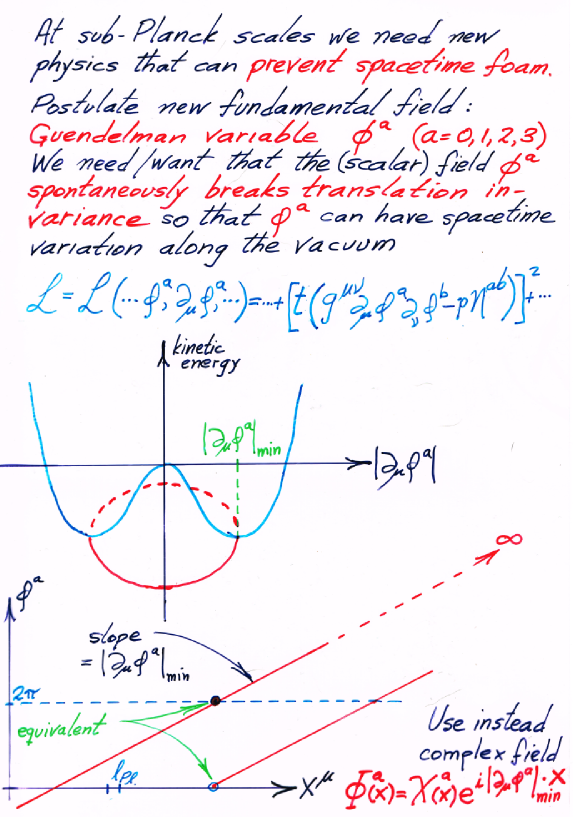
Figure 1: At scales $a<<l_{Pl}$ we postulate a new fundamental field $\Phi$ that explicitly breaks translational symmetry in the vacuum.

Maintaining the constant vacuum value $|\partial_{\mu}\phi^{a}|_{min}$ for the gradient of $\phi^{a}$ in all of spacetime would lead to divergent values of the fields $\phi^{a}$ at large distances. Therefore we take the new fundamental fields to be the complex field $\Phi^{a}$ ($a=0,1,2,3)$

$$\Phi^{a}(x^{0},x^{1},x^{2},x^{3})\equiv\Phi^{a}(x)=\chi^{a}(x)e^{i(\partial_{\mu}\phi^{a})x}.$$ (14)

For the moment we assume that the modulus $\chi^{a}(x)$ has the constant value $\chi_{0}$. In the vacuum it is the gradient of the fundamental field $\phi^{a}(x)$ which has the value $|\partial_{\mu}\phi^{a}|_{min}$ in the vacuum, i.e.,

$$\Phi^{a}_{vac}(x)=\chi^{a}_{0}e^{i(|\partial_{\mu}\phi^{a}|_{min})x}$$ (15)

We can also say that the condition for having the vacuum value $|\partial_{\mu}\phi^{a}|_{min}$ for the gradient is that planes corresponding to adjacent equal values of the complex field $\Phi^{a}(x)$ are separated in spacetime by a (constant) distance $2\pi/|\partial_{\mu}\phi^{a}|_{min}$. Fig. 2 shows the variation of the field component $\Phi^{1}$ as a function $x^{1}$

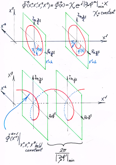
Figure 2: The top part of the figure shows the value of the complex field $\Phi^{1}(x^{1})$ at the arbitrary values $x^{1}=k$ and $x^{1}=h$. Really $\Phi^{1}(x^{1})$ stands for $\Phi^{1}(x^{0},x^{1},x^{2},x^{2})|_{x^{0},x^{2},x^{3}\mbox{held constant}}$ In the bottom part of the figure, adjacent identical values of $\Phi^{1}(x^{1})$ define planes of constant $x^{1}$ separated by a distance $2\pi/|\partial_{\mu}\phi^{a}|_{min}$.

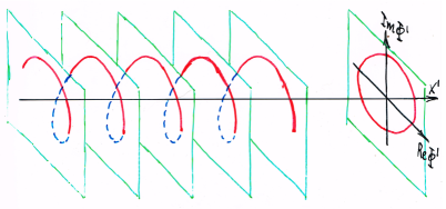
Figure 3: Being in the ground state of the kinetic energy potential of Fig. 1 corresponds to the gradients of the fields having the value $|\partial_{\mu}\phi^{a}|_{min}$ $a=0,1,2,3$ which in turn corresponds to equidistant planes with spacing proportional to $2\pi/|\partial_{\mu}\phi^{a}|_{min}$. Here are shown several such planes for $a=1$.

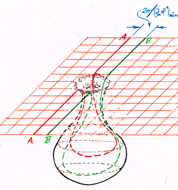
Figure 4: Here we have an almost everywhere regular (i.e., flat spacetime) lattice (here represented by a 2-dimensional grid drawn in perspective). The density of lattice “planes” corresponds to the vacuum value $|\partial_{\mu}\phi^{a}|_{min}$ of the gradient of $\phi^{a}$ which equivalently means that the distance between planes of some chosen constant value of $\Phi^{a}(x)$ is $2\pi/|\partial_{\mu}\phi^{a}|_{min}$. However in the figure there is also an appendix (bubble) that represents a departure from flat spacetime. If we follow two lattice “planes” $\mathbf{A}$ and $\mathbf{B}$ in and out of the appendix we see that underway in the appendix the separation between these “planes” increases because by continuity the same number of lattice “planes” fill a larger volume of spacetime than would be the case without the appendix (i.e., which would be just the “volume” corresponding to the appendix mouth). Hence the density of lattice planes decreases in the appendix to a value $|\partial_{\mu}\phi^{a}|<|\partial_{\mu}\phi^{a}|_{min}$ which corresponds to an excitation relative to the vacuum state (see Fig. 1). Departures from flat spacetime costs energy.

So the requirement of being at the minimum of the potential in Fig. 1 (i.e., $\partial_{\mu}\phi^{a}=|\partial_{\mu}\phi^{a}|_{min}$) defines a (constant) density of planes each of which corresponds to the same value of $\Phi^{1}$. Fig. 3 shows a section of such planes perpendicular to the $x^{1}$ axis.

There are similar planes for the other three spacetime axes. Together this system of planes define a lattice with a lattice constant equal to $2\pi/|\partial_{\mu}\phi^{a}|_{min}$ corresponding to the vacuum value for the gradients of the new fundamental fields.

So we have seen that an action containing positive quartic and negative quadratic terms in the gradient of the new proposed fundamental fields $\phi^{a}$ (see 13) favours the maintenance of a constant density of lattice points with lattice constant $2\pi/|\partial_{\mu}\phi^{a}|_{min}$. Any departure from this vacumm density of lattice points (or planes) costs energy because it corresponds to moving away from the minimum at $|\partial_{\mu}\phi^{a}|=|\partial_{\mu}\phi^{a}|_{min}$.

This is the property that we need: an action that fixes the density of lattice points in the sense explained above. In Fig. 4 we show a (locally 2-dimensional) appendix that opens off of an otherwise 2-dimensional (flat space) lattice with an almost everywhere fixed density of lattice points (or planes) separated by the distance $2\pi/|\partial_{\mu}\phi^{a}|_{min}$. By continuity the lattice planes that go into the appendix must emerge again and rejoin the flat spacetime lattice planes from which they originated.

The crucial point is that the appendix increases the “volume” of spacetime from that corresponding to area of mouth of the appendix to the larger area of the interior of the appendix. But by continuity the number of lattice planes entering and leaving the appendix is the same as the number of planes that enter and leave the area of the appendix mouth without the appendix. Hence the density of lattice planes (or points) decreases within the appendix relative to the density within the area of the mouth without the appendix.

So the presence of the appendix relative to not having it lowers the density of lattice points in the neighborhood of the appendix. Within the appendix the lattice constant becomes larger than $2\pi/|\partial_{\mu}\phi^{a}|_{min}$. This forces the system away from the minimum at $|\partial_{\mu}\phi^{a}|_{min}$ in the potential shown in Fig. 1. Having the appendix costs energy. Energetically flat spacetime is favoured.

Notice that with an action of the form 13 used in our the pivotal relation Eqn. (5) is recovered as an equation of motion upon taking a variation w.r.t. $g^{\mu\nu}$

6 The Emergence of Genearl Relativity as an Effective Theory at Planck Scale

When the new fundamental fields are introduced as the metric in Eqn. (5) we have flat spacetime down to arbitrarily small scales $a<<l_{Pl}$. And a consequence we have seen that the Riemann curvature vanishes identically irrespective of what action is used.

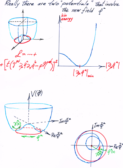
Figure 5: The complex field has two degrees of freedom. In addition to the $\phi$-fields already discussed there is also the $\chi(x)$. In the vacuum this degree of freedom is not excited and can be thought of as a soliton with constant topology.

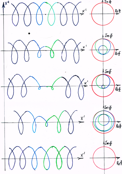
Figure 6: If the $\chi(x)$ degree of freedom is sufficiently excited, the soliton can lose (or gain) a winding. Thinking of the lattice discussed above, changes in the winding number for a soliton can be thought of as the introduction of a crystal defect (dislocation line). It is known (see references to Hagen Klienert) that Einsteinian general relativity can be formulated as a “world crystal” that has dislocation and disclination line defects that give rise to respectively torsion and curvature. This presents a way that the usual general relativity can emerge as an effective theory at say the Planck scale. Recall that at scales $a<<l_{Pl}$ where our new fundamental fields are important spacetime is identically flat. So phenomenologically we need a mechanism by which general relativity appears at roughly Planck scale.

Now the question is how do we regain general relativity when we go up to the Planck scale? Here we rely heavily on the work[5] of Hagen Kleinert. In the special case of the model considered above we have seen how the action defines a spacetime a lattice of constant density $|\partial_{\mu}\phi^{a}|_{min}$ consisting of planes corresponding to equal values of the the new fundamental complex field $\Phi^{a}(x)$. Now we think of this lattice as the “world crystal” of Kleinert. Curvature (and torsion if desired) can be introduced respectively as line dislocation and line disclination defects. Fig. 6 suggests in a soliton model how a dislocation defect can come about by the loss of a soliton winding. Kleinert demonstrates that the introduction of disclination defects in a regular world crystal by the use multivalued coordinate transformations reproduces general relativity in full. We envision this happening at roughly the Planck scale.

References

• [1] C.ย Misner, K.ย S.ย Thorne, and J.ย A.ย Wheeler,โ€œGravitationโ€, San Francisco: W. H. Freeman (1973), ISBN 0716703440. See chapter 43 for superspace and chapter 44 for spacetime foam; C.ย Misner and J.ย A.ย Wheeler, โ€Classical physics as geometryโ€, Ann. Phys. 2 (6): 525 (1957), Bibcode 1957 AnPhyโ€ฆ2..525M. doi:10.1016/0003-4916(57)90049-0, online version (subscription required)
• [2] Wheeler, John Archibald (1963), Geometrodynamics. New York: Academic Press, LCCN 62-013645; J.ย Wheeler (1960) โ€Curved empty space as the building material of the physical world: an assessmentโ€, in Ernest Nagel (1962) Logic, Methodology, and Philosophy of Science, Stanford University Press; J.ย Wheeler (1961) โ€Geometrodynamics and the Problem of Motionโ€, Rev. Mod. Physics 44 (1): 63, Bibcode 1961RvMPโ€ฆ33โ€ฆ63W. doi:10.1103/RevModPhys.33.63. online version (subscription required); J.ย Wheeler (1957), โ€On the nature of quantum geometrodynamicsโ€, Ann.ย Phys.ย 2 (6): 604.
• [3] M.ย Lehto, H.ย B.ย Nielsen and M.ย Ninomiya, โ€œTime Translational Symmetry,โ€ Phys.ย Lett.ย Bย 219 (1989) 87; โ€œSemilocality Of One-dimensional Simplicial Quantum Gravity,โ€ Nucl.ย Phys.ย Bย 289 (1987) 684; โ€œDiffeomorphism Symmetry In Simplicial Quantum Gravity,โ€ Nucl.ย Phys.ย Bย 272 (1986) 228; โ€œPregeometric Quantum Lattice: A General Discussion,โ€ Nucl.ย Phys.ย Bย 272 (1986) 213; โ€œA Correlation Decay Theorem At High Temperature,โ€ Commun.ย Math.ย Phys.ย ย 93 (1984) 483.
• [4] E.ย I.ย Guendelman, Non Singular Origin of the Universe and its Present Vacuum Energy Density, arXiv: 1103.1427v2 [gr-qc] 15 May 2011 and references therein.
• [5] Hagen Kleinert, Multivalued Fields in Condensed Matter, Electromagnetism and Gravitation, World Science Publishing Co. Pte. Ltd. (2008) and references therin.