randomized maximum-contrast selection:
subagging for large-scale regression

Abstract

We introduce a very general method for sparse and large-scale variable selection. The large-scale regression settings is such that both the number of parameters and the number of samples are extremely large. The proposed method is based on careful combination of penalized estimators, each applied to a random projection of the sample space into a low-dimensional space. In one special case that we study in detail, the random projections are divided into non-overlapping blocks; each consisting of only a small portion of the original data. Within each block we select the projection yielding the smallest out-of-sample error. Our random ensemble estimator then aggregates the results according to new maximal-contrast voting scheme to determine the final selected set. Our theoretical results illuminate the effect on performance of increasing the number of non-overlapping blocks. Moreover, we demonstrate that statistical optimality is retained along with the computational speedup. The proposed method achieves minimax rates for approximate recovery over all estimators using the full set of samples. Furthermore, our theoretical results allow the number of subsamples to grow with the subsample size and do not require irrepresentable condition. The estimator is also compared empirically with several other popular high-dimensional estimators via an extensive simulation study, which reveals its excellent finite-sample performance.

1 Introduction

In recent years, statistical analysis of massive data sets has become a subject of increased interest. Modern data sets, often characterized by both high-dimensionality and massive sample sizes, introduce a range of unique computational challenges, including scalability and storage bottlenecks (Fan et al., 2013). Due to the associated storage and computational constraints, the number of data points from the original sample that can be processed will be severely limited (Fithian and Hastie, 2014). In such settings, it becomes natural to employ techniques based on random subsets of the original data that are of a very small size.

Classical ideas of bootstrap (Efron, 1979), aggregation (Breiman, 1996) and subsampling (Politis et al., 2001) are the first that come to mind. However, the key limitation of the traditional bootstrap is that resamples typically have the same order of magnitude and size as the original data. In large-scale settings, $n$ and $p$ are often simultaneously large; orders of magnitude of $10^{6}$ or more are not uncommon. Hence, even computation of a simple point estimate on the full data set can be an issue. Moreover, repeated evaluations of the resamples are likely to face the same set of computational and storage challenges as the original problem.

Subsampling provides a viable alternative, as it only requires computations of samples potentially much smaller than the original data. However, subsampling is quite sensitive to the choice of the subsample size (Samworth, 2003): the smaller the subsample size is, the larger the variance of the estimates. Kleiner et al. (2014) propose an alternative approach called bag of little bootstraps, which combines bootstrap with smaller order subsampling and demonstrate that for the purpose of estimating continuous parameters, such method retains bootstrap-like convergence rates. In this work, we consider all of the above mentioned methods in the context of the support recovery and large-scale regression.

We propose a method that operates with a large number of subsamples, each of a very small size, that can approximately retrieve the support set of the regression parameters. We employ an approach of subsample bootstrap aggregation (subagging) and illustrate how to aggregate estimators in order to produce stable approximations of the support set $S$, without requiring the widely used Irrepresentable condition (van de Geer and Bühlmann, 2009). The key is to compute estimates, at non-overlapping subsamples using randomized bootstrap and then exploit the randomization to enlarge support sets of those estimates. In this way, we ensure uniformity of the results, obtained across subsamples and avoid the potentially harmful effects of smaller order subsampling.

We consider the simple linear model

$$\mathbf{Y}=\mathbf{X}\boldsymbol{\boldsymbol{\beta}}^{*}+\boldsymbol{\varepsilon},$$ (1)

where $\mathbf{Y}\in\mathbb{R}^{n}$, $\mathbf{X}\in\mathbb{R}^{n\times p}$ and both $n$ and $p$ are very large numbers, possibly of the order of hundreds of thousands or millions. The noise vector $\boldsymbol{\varepsilon}$ is assumed to be i.i.d. and independent of $\mathbf{X}$. We assume that the vector $\boldsymbol{\boldsymbol{\beta}}^{*}$ is such that its support set $\mbox{supp}(\boldsymbol{\boldsymbol{\beta}}^{*})=S\subseteq\{1,\cdots,p\}$ describes a particular subset of important variables for the linear model (1), for which we then assume $|S|\ll p$. The method presented here is quite intuitive: we partition the dataset of size $n$ randomly into $d$ equal subsets of size $N\ll\min\{n,p\}$ and compute the penalized regression estimate for each of the $i=1,\dots,d$ subsets independently, using a careful choice of the regularization parameter $\lambda_{N}$. The estimates are subsequently averaged using a new multiple voting scheme that shrinks high variability in the estimates.

As computations are done independently of each other, the proposed method is especially suited for implementation across distributed and parallel computing platforms, often used for processing of large-scale data. Distributed approaches based on bootstrap aggregation (Breiman, 1996) have been studied by several authors, including Bühlmann and Yu (2002) for least-squares algorithms, Bach (2008) for bootstrapped Lasso algorithm, McDonald et al. (2010) for perceptron-based algorithms, Kleiner et al. (2014) for distributed versions of a bootstrap, Zhang et al. (2012) for convex optimization and Zhang et al. (2013) for kernel ridge regression algorithm. However, support recovery guarantees for subsampled approaches of a smaller scale, have not been analyzed much in the existing literature. Recent proposals include Bayesian median of subsets Minsker et al. (2014) and related median of subsets Wang et al. (2014). However, both approaches work with subsamples with sizes proportional to $n$.

The fundamental observations that underpins our proposal is the fact that naive aggregation of the estimators computed on the small subsamples, is not sensible, since most of the subsamples will typically destroy the structure in the data. Nevertheless, such estimators have great flexibility in a choice of the regularization parameter. Our theoretical analysis demonstrates that, even though each subsampled estimator is computed only on a very small fraction of the samples, it is essential to regularize such estimators as if they had all $n$ samples. As a result of that, each sub-problem is under-regularized, which allows for the small bias in estimation, but causes an adverse blow-up in the variance. Hence, a simple majority vote of the retained sets can be highly suboptimal; instead, we argue that the voting should be chosen to minimize the worst case risk. We show that such voting scheme, named maximal-contrast voting, sufficiently reduces the variance of under-regularization. Our main theorem shows that, while achieving computational speedup the proposed method retains statistical optimality; it achieves minimax rates, over all estimators using the set of $n$ samples.

Our theoretical results are divided into three parts. In the first, we consider one randomized subsample estimator and quantify the difference between the selected set of such one subsample estimator and the Lasso estimator computed on the data of the full size $n$. We then consider minimax-contrast aggregation of such randomized estimators computed on non-overlapping blocks. Under a condition implied by the widely-used restricted eigenvalue assumption (Bickel et al., 2009), we can then control the difference between the selected set of the aggregated estimator and the true support set $S$, as a function of terms that depend on the number of non-overlapping blocks, the pairwise block distance, as well as the size of the each block and terms that diminish when the number of blocks grow. Furthermore, we establish minimax optimality of the proposed method. The final part of our theory gives risk bounds on the naive bagging of Lasso estimators named Bootstrapped Lasso in Bach (2008), namely its inability to retrieve support set when the number of blocks grows.

We briefly introduce the notation used throughout the paper. Let $I$ and $J$ be two subsets of $\{1,\cdots,n\}$ and $\{1,\cdots,p\}$ respectively. For any set $S$ we use $|S|$ to denote its cardinality. For any vector $\mathbf{x}$, let $\mathbf{x}_{J}\in\mathbb{R}^{|J|}$ denote its sub vector with coordinates belonging to $J$. We use notation $\|\mbox{\bf x}\|$, $\|\mbox{\bf x}\|_{1}$ and $\|\mbox{\bf x}\|_{\infty}$ to denote $L_{2}$, $L_{1}$ and $L_{\infty}$ norms respectively, of a vector x. For any matrix $\mathbf{A}$, let $\mathbf{a}^{j}$ denote its $j$-th column vector, and let $\mathbf{A}_{I,J}$ denote a matrix formed by the rows and columns of $\mathbf{A}$, which belong to the set $I$ and $J$, respectively. Shorthand notation $\mathbf{A}_{I}$ stands for $\mathbf{A}_{I,\{1,\cdots,p\}}$. We also use $\phi_{\min}(\mathbf{A})=\lambda_{\min}(\mathbf{A}^{T}\mathbf{A})$ and $\phi_{\max}(\mathbf{A})=\lambda_{\max}(\mathbf{A}^{T}\mathbf{A})$ with $\lambda_{\min}$ and $\lambda_{\max}$ denoting minimal and maximal eigenvalue, respectively. We denote with $\kappa(\mathbf{A}^{T}\mathbf{A})$ the conditioning number of matrix $\mathbf{A}$, and define it as $\phi_{\max}(\mathbf{A})/\phi_{\min}(\mathbf{A})$. We use $\|\mbox{\bf A}\|$ to denote the operator norm of a matrix A. Note that $\lambda_{N}$ and $\lambda_{n}$ denote tuning parameters of Lasso problems, computed over subsample of size $N$ and full sample of size $n$, respectively.

The rest of the paper is organized as follows. Section 2 describes the proposed weighted small sample bagging of Lasso estimators. Theorems 1 and 2 of Section 3, discuss the difference between the estimated sparsity sets of the sub-Lasso and the Lasso estimators. Subsection 3.2 discusses theoretical findings on support recovery properties of the weighted subagging, with the main result summarized in Theorem 3. Theorem 4 develops novel minimax rates for approximate support recovery. Subsection 3.3 outlines the inefficiency of classical subagging of Lasso estimators ,with the main results summarized in Theorems 6 and 7. Finally, in Section 4 we provide details and results of the implementation of our method on the simulated data.

2 Randomized Maximum-Contrast Selection

We start by describing our sample partitioning and defining the relevant notation. Let $I=\{1,\cdots,n\}$ denote the sample index set, which we divide into a group of disjoint subsets each of size $N\ll n$. Although we are mostly interested in subsets of a much smaller order than $n$, the exposition of the method does not depend on the choice of $N$. In this sense, the complete dataset $\{(Y_{1},\mbox{\bf X}_{1}),(Y_{2},\mbox{\bf X}_{2})\cdots,(Y_{n},\mbox{\bf X}_{n})\}$ is split evenly and uniformly at random into many small, disjoint subsets. We consider $d$ of such subsets, i.e.

$$(\mathbf{Y}_{I_{i}},\mathbf{X}_{I_{i}})=\bigl{\{}(Y_{i_{1}},\mbox{\bf X}_{i_{1}}),\cdots,(Y_{i_{N}},\mbox{\bf X}_{i_{N}})\bigl{\}},$$ (2)

for $i=1,\cdots,d$ and allow $d$ to grow with $n$.

Let the weighted sub-Lasso estimator ${\hat{\boldsymbol{\beta}}}_{i:k}(\lambda_{N})$ be defined as

$${\hat{\boldsymbol{\beta}}}_{i:k}(\lambda_{N})=\arg\min_{\boldsymbol{\beta}}\biggl{\{}\frac{1}{2n}\bigl{\|}\mbox{\bf D}_{\sqrt{\mathbf{w}_{k}}}\mathbf{Y}_{I_{i}}-\mbox{\bf D}_{\sqrt{\mathbf{w}_{k}}}\mathbf{X}_{I_{i}}\boldsymbol{\beta}\bigl{\|}^{2}\ +\lambda_{N}\|\boldsymbol{\beta}\|_{1}\biggl{\}},$$ (3)

where $\mbox{\bf D}_{\mathbf{w}_{k}}\in\mathbb{R}^{N\times N}$ is a diagonal matrix with a vector of random weights, $\mathbf{w}_{k}\in\mathbb{R}^{N}$ on its diagonal. Index $k=1,\dots,K$ enumerates the number of random draws of the weight vector $\mathbf{w}$. Note that ${\hat{\boldsymbol{\beta}}}_{i:k}(\lambda_{N})$ is computed using only observations within one subset of the data. Yet, for fixed and discrete choice of $\mathbf{w}_{k}$, ${\hat{\boldsymbol{\beta}}}_{i:k}(\lambda_{N})$ can be rewritten as the solution to an $n\times p$ problem

$${\hat{\boldsymbol{\beta}}}_{i:k}(\lambda_{N})=\arg\min_{\boldsymbol{\beta}}\left\{\frac{1}{2n}\left\|\tilde{\mbox{\bf Y}}-\tilde{\mbox{\bf X}}_{i:k}\boldsymbol{\beta}\right\|^{2}+\lambda_{N}\|\boldsymbol{\beta}\|_{1}\right\},$$

with $\tilde{\mathbf{X}}_{i:k}^{T}\in\mathbb{R}^{p\times n}$ defined as

$$\tilde{\mathbf{X}}_{i}^{T}=[\mathbf{X}_{i_{1}}^{T},\cdots,\mathbf{X}_{i_{1}}^{T},\cdots,\mathbf{X}_{i_{N}}^{T},\cdots,\mathbf{X}_{i_{N}}^{T}],$$ (4)

with the rows $\mathbf{X}_{i_{j}}\in\mathbb{R}^{1\times p}$ repeated $w_{k,i_{j}}$ times, each for $j\in 1,\cdots,N$ and $k=1,\cdots,K$. In other words, ${\hat{\boldsymbol{\beta}}}_{i:k}(\lambda_{N})$ minimizes the penalization problem, computed using a random projection of the original data, where all the features are kept and the sample space is projected into a low-dimensional space of size $N$. The proposed projection, places a constraint that the number of distinct observations $N$ is fixed, non-random and much smaller than $n$; different from the Efron’s traditional bootstrap method which has a random number of distinct observations. Furthermore, we require the following condition on the random vector $\mathbf{w}_{k}$, for all $k=1,\dots,K$.

Condition 1.

Let $\mathbf{w}=(w_{1},\dots,w_{N})$ be a random vector, such that $w_{1},\dots,w_{N}$ are exchangeable random variables and are independent of the data $(\mbox{\bf Y},\mbox{\bf X})$. Moreover, $w_{1},\dots,w_{N}$ are such that $\sum_{j=1}^{N}w_{j}=n$ and $P(w_{1}>0)=1$. Additionally, for $\mathbf{w}_{2}^{2}=\int_{0}^{e^{2n}}P_{w}\left(\max_{1\leq j\leq N}w_{j}\geq\frac{1}{2}\log t\right)dt$, let $\mathbf{w}_{2}$ satisfy $\log\mathbf{w}_{2}\leq p^{n/N}/n$ almost surely.

Condition 1 is inspired by similar conditions imposed for the weighted bootstraps (Præstgaard and Wellner, 1993). However, traditional weights do not fit the Condition 1 as they typically follow the Multinomial $\mathcal{M}_{n}(N,(\frac{1}{n},\cdots,\frac{1}{n}))$ distribution of dimension $n\geq N$. If we reverse the roles of $n$ and $N$, they can easily be adapted to the Condition 1, with vector $\mathbf{w}_{k}$, drawn from the Multinomial distribution $\mathcal{M}_{N}(n,(\frac{1}{N},\cdots,\frac{1}{N}))$. Each random projection of the original data is data of size $n$, drawn with replacement on $N\ll n$ fixed, original data points. Kleiner et al. (2014) use these resamples to average continuous estimators. In contrast, our focus is the support recovery in large scale and potentially high dimensional problems. Other examples of randomized schemes that satisfy Condition 1, include a Balanced Pólya urn scheme (Antognini and Giannerini, 2007) and a coupling of Poisson and Multinomial distribution; the first includes a Pólya urn scheme with a strategy guaranteeing that each ball color is represented at least once whereas the second scheme includes a randomized game of throwing $n$ balls into $N$ urns, and repeating the throws until all the balls are in urns.

For the simplicity in presentation we impose the following finite moment condition on the noise vector of the linear model (1). Nevertheless, we believe all the results of the manuscript extend to sub-Gaussian errors.

Condition 2.

The noise vector $\boldsymbol{\varepsilon}$, (1), is such that $E_{\varepsilon}|\varepsilon_{i}|^{r}\leq r!\sigma^{2}c^{r-2}/2$ for every $r\geq 2$ (and all $i$) and some constants $c<\infty$ and $\sigma^{2}<\infty$.

Let the indices $\{1,\dots,d\}$ be split into $b$ blocks of $m$-pairs; in particular, $b$ and $m$ satisfy $d=bm$. The number of subsamples, $d$, is allowed to grow with $n$; it depends on $n$ through $b$. Constant $m$ allows for additional flexibility in estimation. Next, we introduce the maximal-contrast selection, a variant of stability selection, where the subsamples are drawn as $N\ll n$, $m$ complementary pairs from $\{1,\dots,n\}$. Thus the procedure outputs, $b$ of such $m$-pairs index sets $\{I_{mq+1-l};q=1,\dots,b,l=1,\dots,m\}$, where each $I_{mq+1-l}$ is subset of $\{1,\dots,n\}$ of size $N$ and $I_{mq+1-1}\cap\dots\cap I_{mq+1-m}=\emptyset$. A special case of the above sets, with $m=1$ and $m=2$ are the sets of Meinshausen and Bühlmann (2010); Wang et al. (2014) and the sets of Shah and Samworth (2013), respectively. However, both are based on the subsets that are of the size proportional to $n$. As we allow $d$ to grow with $n$, our procedure includes subsamples of a much smaller order. For such cases, simply applying existing methods above leads to “select all” or “select none” vote (see Theorem 6 for a detailed proof). We show in Theorem 1 below that subsamples of a much smaller order cause blow-up in the variance of the estimated non-zero sets of ${\hat{\boldsymbol{\beta}}}_{i:k}(\lambda_{N})$; that is, the variance of the sets

$$\hat{S}_{i}(\lambda_{N},k)=\left\{1\leq j\leq p:{\hat{\beta}}_{i:k,j}(\lambda_{N})\neq 0\right\},$$

for each fixed vector $\mathbf{w}_{k}$, $k=1,\dots,K$, is large. Hence, naive estimators above fail and we aim to improve them. After $K$ random draws of $\mathbf{w}_{\mathbf{k}}$, for each subsample $I_{i}$, we obtain $K$ sets $\hat{S}_{i}(\lambda_{N},1),\dots,$ $\hat{S}_{i}(\lambda_{N},K)$. Initially, we compute the selection of variable $j$ in a union of those $K$ sets. Next we compute a minimax majority vote across $m$-pairs of these unions, each computed on the non-overlapping subsamples. The minimax majority vote estimator is defined as

$$\pi_{j}^{*}(\lambda_{N},b,m,K)=\frac{1}{\sqrt{b}(\sqrt{b}+1)}\sum_{q=1}^{b}\mathbbm{1}\left\{j\in\cap_{l=1}^{m}\cup_{k=1}^{K}\hat{S}_{mq+1-l}(\lambda_{N},k)\right\}+\frac{1}{2}\frac{1}{\sqrt{b}+1}.$$ (5)

Whenever possible we suppress $b,m,K$ from $\pi_{j}^{*}(\lambda_{N},b,m,K)$ and write $\pi_{j}^{*}(\lambda_{N})$ for short. This estimator arises as a solution to the minimax estimation of a mean of a Bernoulli trial (see Chapter 5, Example 1.7 of Lehmann and Casella (1998) for more details). For small values of $b\leq 40$ and all possible values of $p_{j}$, $\pi_{j}^{*}(\lambda_{N})$ has a larger bias, (bounded with $2^{-1}(1+\sqrt{b})^{-1}$ in absolute value) but a smaller variance compared to the maximum likelihood estimator.

Next, we define the weighted maximum-contrast subagging estimator $\widehat{{\boldsymbol{\beta}}}^{a}(\lambda_{N})$ to be $\widehat{{\boldsymbol{\beta}}}^{a}_{j}(\lambda_{N})=0$ if $j\notin\hat{S}_{\tau}$,

$$\hat{S}_{\tau}(\lambda_{N})=\left\{1\leq j\leq p:\pi_{j}^{*}(\lambda_{N})\geq\tau\right\},$$

with appropriately chosen thresholding parameter $\tau$. Otherwise, when $j\in\hat{S}_{\tau}$

$$\widehat{{\boldsymbol{\beta}}}^{a}_{j}(\lambda_{N})=K^{-1}d^{-1}\sum_{i=1}^{d}\sum_{k=1}^{K}{\hat{\beta}}_{i:k,j}(\lambda_{N}).$$ (6)

Observe that the aggregated estimator $\widehat{{\boldsymbol{\beta}}}^{a}_{j}(\lambda_{N})$ is a random and dependent on the number of random draws $K$, the number of blocks $b$ and the distance between blocks $m$. We emphasize here the additional flexibility afforded by not pre-specifying the voting threshold $\tau$ to be 1/2; or the size of the pairs $m$ to be 1.

The threshold value $\tau$ is a tuning parameter whose influence is very small. For practical values in the range of, say, $\tau\in(0.25,0.75)$, results tend to be very similar. The choice of $m$ is more intricate. Large values of $m$ lead to the smaller number of both false and true positives. However, in such cases, they simultaneously lead to smaller values of $b$. Such small values are especially suited for the estimator (6) as they cause greater value of the bias; which in turn leads to an improvement of the selection. For such choices of $m$, we advocate a smaller value of the tuning parameter $\tau$. For smaller values of $m$ and hence large values of $b$, the estimator (6) resembles majority vote estimator. However, small $m$ produces a large number of false positives. However, large values of $\tau$ can reduce this bias in selection.

For $m=1,K=1,b=d$ and $\tau=1/2$, the proposed estimator takes on a form of the “majority vote” estimator, so that $\hat{S}_{\tau}(\lambda_{N})$ consists of all $j$ that are included in at least half of the sets $\hat{S}_{i}(\lambda_{N},1)$, $i=1,\dots,d$. Furthermore, for $\tau=1/4(1+\frac{1}{\sqrt{d}+1})>1/4$, $\hat{S}_{\tau}(\lambda_{N})$ consists of all $j$ that are included in at least a quarter of the sets $\hat{S}_{i}(\lambda_{N},1)$, $i=1,\dots,d$. Moreover, for the case of $m=2,K=2,b=\lfloor{d/2}\rfloor$ and $\tau=1/2$, $\hat{S}_{\tau}(\lambda_{N})$ consists of all $j$ that are included in at least half of the sets

$$\{\hat{S}_{i}(\lambda_{N},1)\cup\hat{S}_{i}(\lambda_{N},2)\}\cap\{\hat{S}_{i+\lfloor{d/2}\rfloor}(\lambda_{N},1)\cup\hat{S}_{i+\lfloor{d/2}\rfloor}(\lambda_{N},2)\},\qquad i=1,\dots,\lfloor{d/2}\rfloor.$$

We observe that maximum-contrast selection allows for more structure in the search of the support set. Moreover, $\widehat{{\boldsymbol{\beta}}}^{a}_{j}(\lambda_{N})$ takes the form of a randomized subagging (Bühlmann and Yu, 2002) and a delete$-(n-N)-$jackknife (Efron, 1979) with additional discovery control, suited for a smaller order subsamples and a very large size of the deleted set (with $(n-N)/n\to 1$), respectively.

If we apply Lasso to the full data the estimated set will converge to the true support set only if stringent conditions are imposed. Next section shows that the median-contrast selection does not rely on such heavy assumptions, leading to substantial gains in not only computational time but also feature selection performance. The intuition for this gain is that a large proportion of the subsets of the data does not preserve the structure of the full data; this in turn has a sizable influence on the selected sets. By taking biased estimator with controlled variance and additional randomization steps, we obtain a more uniform model that is not largely influenced by these altered structure of the subsets. As large-scale data typically contain outliers and data contamination, this is a substantial practical advantage.

3 Theoretical Properties

Without loss of generality, from this point on we assume that the columns of $\mathbf{X}$ have unit $l_{2}$ norm. Let $a\geq 1$ be a constant. Because of the regularization, the following cone set is important:

$$\mathbb{C}(a,S)=\left\{\mathbf{v}\in\mathbb{R}^{p}:\mathbf{v}\neq 0,\|\mathbf{v}_{S^{c}}\|_{1}\leq a\|\mathbf{v}_{S}\|_{1}\right\}.$$

The Restricted Eigenvalue $\zeta_{N}$ of the matrix $[\sqrt{\mathbf{w}}_{k}\mbox{\bf X}]$ for a vector $\mathbf{w}_{k}\in\mathbb{R}^{N}$ and a design matrix of a partitioned data $\mbox{\bf X}\in\mathbb{R}^{N\times p}$ is defined in Condition 3.

Condition 3.

Let $\mathbf{w}_{k}\in\mathbb{R}^{N}$ be vectors of weights. For a matrix $\tilde{\mathbf{X}}_{i:k}\in\mathbb{R}^{n\times p}$ as in (4), and $a>1$, there exists a positive number $\zeta_{N}>0$ such that for all $|S|\leq 2s$

$$\zeta_{N}=\min_{\mathbf{v}\in\mathbb{C}(a,S)}\frac{\|\tilde{\mathbf{X}}\mathbf{v}\|_{2}}{\sqrt{n}\|\mathbf{v}_{S}\|_{2}}.$$

The restricted eigenvalues $\zeta_{N}$ are variants of the restricted eigenvalue introduced in Bickel et al. (2009) and of the compatibility condition in van de Geer and Bühlmann (2009). In the display above $\|\tilde{\mathbf{X}}\mathbf{v}\|_{2}^{2}=\sum_{l\in I_{i}}w_{k,l}(\mathbf{X}_{l}\mathbf{v})^{2}$ for any realization $k$ of the weight vector $\mathbf{w}_{k}$. We use subscript $N$ in $\zeta_{N}$ to denote the number of distinct rows of the matrix $\tilde{\mathbf{X}}_{i:k}$. As long as the tail of the distribution of $X$ decays exponentially, column correlation is not too large and $N\geq|S|\log p$, the condition above holds with high probability (Raskutti et al., 2010).

It is well established that the necessary condition for the exact recovery of penalized methods consist of the Irrepresentable condition (van de Geer and Bühlmann, 2009).

Condition 4 (IR$(n)$).

The design matrix $\mathbf{X}\in\mathbb{R}^{n\times p}$ satisfies IR$(n)$ condition if the following holds $\left\|\mathbf{X}_{{S}^{c}}\mathbf{X}_{S}(\mathbf{X}_{S}^{T}\mathbf{X}_{S})^{-1}\mbox{sign}({\boldsymbol{\beta}}^{*})\right\|_{\infty}<1.$

The symbol IR$(n)$ denotes the number of rows in the design matrix $\mathbf{X}$, with $n$ denoting the sample size. When IR$(N)$ is assumed to hold for every subsampled dataset, then each of the penalized regression estimates $\hat{}\mbox{\boldmath$\beta$}_{i:k}(\lambda_{N})$ would recover the set $S$ with high probability – a commonly used condition in an existing literature (Wang et al., 2014). A far more interesting scenario is to allow deviations from IR$(N)$ condition. With subsamples of a very small size, $N\ll p$ and $N\ll n$, imposing such conditions on each subsample is not realistic; most of the subsamples will not preserve the original data structure. Instead, we examine different properties of the design and the sub design matrices without imposing IR$(N)$ condition.

Lemma 1.

Let Condition 3 hold. Let $A\subseteq\{1,\dots,p\}$ that is of the size $|A|=r\leq 2s$ and let $I\subseteq\{1,\dots,n\}$ be of the size $|I|=N$. Assume that the matrix $\mathbf{X}_{I}\in\mathbb{R}^{N\times p}$ satisfies Condition 3 with $a=3$. Then, for every $j\notin A$ ,

$$\|\mathbf{X}_{I,A}^{T}\mathbf{X}_{I,j}\|_{2} \leq \zeta_{N}^{-3},$$ (7)

$$\left\|(\mathbf{X}_{I,A}^{T}\mathbf{X}_{I,A})^{-1}\mathbf{X}_{I,A}^{T}\mathbf{X}_{I,j}\right\|_{1}^{2} \leq r/\zeta_{N}^{2}.$$ (8)

Observe that, under Condition 3, a result of Lemma 1 is much weaker than the Irrepresentable condition IR$(N)$, as $r\geq\zeta_{N}^{2}$ and is possibly dependent on $n$.

The following lemma characterizes uniform deviation of a randomized weighted sum of negatively correlated random variables and is critical in obtaining finite sample properties; see Theorem 3 below. To the best of our knowledge there is no similar result in the literature. We use $\langle\cdot,\cdot\rangle_{n}$ to denote the empirical inner product, i.e. $\langle\mbox{\bf u},\mbox{\bf v}\rangle_{n}=\frac{1}{n}\mbox{\bf u}^{T}\mbox{\bf v}$, for two vectors $\mbox{\bf u},\mbox{\bf v}\in\mathbb{R}^{p}$.

Lemma 2.

Let $\mathbf{w}=(w_{1},\cdots,w_{N})$ be a vector of weights that satisfies Condition 1. Let the error $\boldsymbol{\varepsilon}$ satisfy Condition 2. Then, all $i=1,\dots,d$ there exists a sequence $u_{n}$ of non-negative real numbers, such that

$$\mathbb{P}\biggl{(}\Bigl{|}\left\langle\mbox{\boldmath$\varepsilon$}_{I_{i}},\mbox{\bf D}_{\mathbf{w}}\mbox{\bf X}_{I_{i}}\right\rangle_{n}\Bigl{|}>u_{n}\biggl{)}\leq\exp\left\{N\log\mathbf{w}_{2}-\frac{n^{2}u_{n}^{2}}{2\sigma^{2}N\|\mbox{\bf X}_{I_{i}}\|_{\infty,2}+2ncu_{n}\|\mbox{\bf X}_{I_{i}}\|_{\infty,\infty}}\right\},$$

with $\mathbf{w}_{2}$ defined in Condition 1. In display above, $\|\mbox{\bf X}_{I_{i}}\|_{\infty,2}:=\max{}\Bigl{\{}{X}_{I_{i}j}^{2}:I_{i}\subset\{1,\cdots,n\},\Bigl{.}$ $\Bigl{.}|I_{i}|=N,1\leq j\leq p\Bigl{\}}$ and $\|\mbox{\bf X}_{I_{i}}\|_{\infty,\infty}:=\max\Bigl{\{}|{X}|_{I_{i}j}:I_{i}\subset\{1,\cdots,n\},|I_{i}|=N,1\leq j\leq p\Bigl{\}}$.

Lemma 2 represents a uniform, nonasymptotic exponential inequality for a sum of negatively correlated random variables. Compared with other concentration inequalities (Kontorovich and Ramanan, 2008; Permantle and Peres, 2014), it holds for continuous random variables which are negatively correlated. Moreover, its independence of dimensionality $p$ and dependence on $n$, proves to be invaluable for the variable selection properties.

3.1 Support sets

When dealing with “imperfect learners”, an important question is how to aggregate information over all learners. In order to examine the performance of $\widehat{{\boldsymbol{\beta}}}^{a}_{j}(\lambda_{N})$, we first study ${\hat{\mbox{\boldmath$\beta$}}}_{i:k}(\lambda_{N})$ and its ability to recover the support set $S$, for each fixed $k=1,\dots,K$.

Theorem 1.

Let $k=1,\dots,K$ be fixed. Let $\mathbf{w}_{k}$ be a vector of weights satisfying Condition 1. Let the error $\boldsymbol{\varepsilon}$ satisfy Condition 2. Assume that the matrix $\mathbf{X}_{I_{i}}$ satisfies Condition 3 with $a=3$ and $i=1,\dots,d$. Then, for every $k=1,\cdots,K$, with a choice of $c_{1}\sigma\sqrt{\log p/n}\leq\lambda_{N}\leq c_{2}\sigma\sqrt{\log p/n}$, $c_{1}>0,c_{2}>1$, there exists a constant $c>1$ such that, $P(S\subseteq\hat{S}_{i}(\lambda_{N},k))\geq 1-p^{1-c}.$ Moreover, constants $c_{1},c_{2}$ and $c$ do not depend on $n,p$ or $s$.

The proof of Theorem 1 is in the Appendix. One of the technical challenges is to control the inner product between $\mbox{\bf X}_{I_{i}^{c}}$ and the out-of-sample fit $\mbox{\bf Y}_{I_{i}^{c}}-\hat{}\mbox{\bf Y}_{I_{i}^{c}}$ with $\hat{}\mbox{\bf Y}_{I_{i}^{c}}=\mbox{\bf X}_{I_{i}^{c}}\hat{\boldsymbol{\beta}}_{i:k}(\lambda_{N})$. Theorem 1 has immediate consequences.

Remark 1.

Theorem 1 shows that the sub-Lasso estimator, computed only on a small fraction of the data, requires regularization comparable to that of the complete data – proportional to $\sqrt{\log p/n}$. As $\mathbb{E}[\mathbf{w}_{k}]=(n/N,\dots,n/N)$, existing work on Lasso estimator (Bickel et al., 2009) implies that a regularization of $\sqrt{\log p/N}$ suffices for the purpose of variable selection. Instead, we obtain a regularization of much smaller order to be necessary.

In a different context, Zhang et al. (2013) similarly show that subsampled kernel smoothing with ridge penalty, requires regularization proportional to that of the original data, albeit for prediction purposes.

Next, we compare the selection set of one sub-Lasso estimator and the Lasso estimator computed on the original data defined as

$$\hat{\boldsymbol{\beta}}(\lambda_{n})=\arg\min_{\boldsymbol{\beta}\in\mathbb{R}^{p}}\left\{\frac{1}{2n}\|\mathbf{Y}-\mathbf{X}\boldsymbol{\beta}\|^{2}+\lambda_{n}\|\boldsymbol{\beta}\|_{1}\right\}.$$ (9)

Whenever Condition 4 holds, the Lasso estimator is an oracle estimator; it recovers the correct set with high probability. We show that whenever the Irrepresentable Condition IR$(n)$ holds, and all

$$\lambda_{N}\in(0,{c}\lambda_{n}-\frac{c_{1}}{\sqrt{n}})\cup(nc\lambda_{n}+c^{2}c_{1},\infty),$$

for some universal constants $c>1$ and $c_{1}>0$, the estimated sets of ${\hat{\boldsymbol{\beta}}}_{i:k}(\lambda_{N})$ and ${\hat{\boldsymbol{\beta}}}(\lambda_{n})$ are nested, with probability converging to $1$. Theorem 1, in addition to Condition 4, guarantees that $\hat{S}\subseteq\hat{S}_{i}$, i.e. there exists a constant $c>1$ such that for all $\lambda_{N}\leq{c}\lambda_{n}$,

$$P(\hat{\boldsymbol{\beta}}_{i:k,j}(\lambda_{N})\neq 0)\geq P(\hat{\boldsymbol{\beta}}_{j}(\lambda_{n})\neq 0),\ \ \ j\in S,\ \ \$$ (10)

whereas Theorem 2 and Condition 4 guarantee $\hat{S}\supseteq\hat{S}_{i}$, i.e. for $\lambda_{N}\geq nc\lambda_{n}$,

$$P(\hat{\boldsymbol{\beta}}_{i:k,j}(\lambda_{N})\neq 0)\leq P(\hat{\boldsymbol{\beta}}_{j}(\lambda_{n})\neq 0),\ \ \ j\in S.\ \ \$$ (11)

We obtain the following result.

Theorem 2.

Let $k=1,\dots,K$ be fixed. Let $\mathbf{w}_{k}$ be a vector of weights that satisfies Condition 1. Let the error $\boldsymbol{\varepsilon}$ satisfy Condition 2. Assume that matrix $\bf X$ satisfies Condition 4 and that there exists a positive constant $C^{\prime}$ such that $\lambda_{\max}\left(\frac{1}{n}\mathbf{X}^{T}\mathbf{X}\right)/{\zeta_{n}}\leq C^{\prime}$. Assume that the matrix $\mathbf{X}_{I_{i}}$ satisfies Condition 3 with $a=3$ and $i=1,\dots,d$. Then, for all

$${\lambda_{N}}{} \geq (n+1)\lambda_{n}+\frac{\lambda_{n}C^{\prime 3/2}s^{3/2}}{{\zeta_{n}^{2}\zeta_{N-n}}}+\frac{\sqrt{2}\lambda_{n}C^{\prime 3/2}s^{3/2}}{\zeta_{n}\zeta_{N-n}^{3}}+2\sigma\sqrt{{(n-N)\log p}{}}+2\sigma\sqrt{{4C^{\prime}\log p/n}{}},$$

there exists a constant $c>1$ such that for every $k=1,\cdots,K$, $P(S\supseteq\hat{S}_{i}(\lambda_{N},k))\geq 1-p^{1-c}$.

Hence, the optimal $\lambda_{N}$, according to the Theorem 2, is of the same order as $\sigma\sqrt{\log p}$. In contrast, the optimal $\lambda_{N}$, according to the Theorem 1, is of the order of $\sigma\sqrt{\log p/n}$. Hence, there does not exists a universal choice of $\lambda_{N}$, for a sub-Lasso estimator to have exact support recovery.

Remark 2.

This result provides novel insights into finite sample equivalents of the asymptotic bias of subagging and “majority voting” as presented in Bühlmann and Yu (2002). There the authors suggests that there is asymptotically zero probability that the subsampled Lasso (sub-Lasso) and Lasso estimators have the same sparsity patterns (see Theorem 3.3 therein). Theorems 1 and 2 show show that the given probability is equal to zero. We show more details in Section 3.4.

The immediate consequence is that naive “multiple vote” estimate does not have a single choice of $\lambda_{N}$ that achieves variable selection. Details are presented in Theorem 6.

3.2 Efficiency and optimality

Next, we state the main theorems on the finite sample variable selection property and optimality of the proposed minimax voting scheme (6).

The bootstrap scheme is said to be efficient if it mimics the “behavior” of the original data. In this context, “behavior” can mean many things, like inheriting rates of convergence in the central limit theorem or in the large deviations. In this work, we concentrate on two types of efficiency. The first considers “exact sparse recovery”, where $\hat{S}=S$, for a candidate estimator $\hat{S}$, with high probability. The second considers “approximate sparse recovery”, where the focus is on establishing the following two properties simultaneously

$$P\left(S\subseteq\hat{S}\right)\geq 1-\delta,\mbox{ for }\delta\in(0,1)\qquad E|\hat{S}\cap S^{c}|\leq\varepsilon s/p,\mbox{ for }\varepsilon\in(0,1).$$

Typically, $\delta$ and $\varepsilon$ in the above considerations are numbers which are very close to zero.

Theorem 3.

Let $\mathbf{w}_{k}$ be a vector of weights satisfying Condition 1 for all $k=1,\dots,K$. Let the error $\boldsymbol{\varepsilon}$ satisffy Condition 2. Assume that the matrix $\mathbf{X}_{I_{i}}$ satisfies Condition 3 with $a=3$ and $i=1,\dots,d$. Let the distribution of

$$\left\{\mathbbm{1}\left(j\in\cup_{k=1}^{K}\hat{S}_{i}(\lambda_{N},k)\right),s+1\leq j\leq p\right\},$$

be exchangeable for $\lambda_{N}$ as in (12) and all $i=1,\dots,d$. Moreover, let $\|\mathbf{X}_{I_{i}}\|_{\infty,\infty}\leq c_{2}\sqrt{N/\log p}$, for some constant $c_{2}>1$ and all $1\leq i\leq d$. Then, there exists a bounded, positive, universal constant $c^{\prime}>1$ such that, for

$$\frac{1}{c^{\prime}}\sqrt{\log p/n}\leq\lambda_{N}\leq c^{\prime}\sqrt{\log p/n},$$ (12)

the following holds

$$P(S\subseteq\hat{S}_{\tau}(\lambda_{N}))\geq 1-p^{1-c^{\prime}},$$ (13)

and

$$\sup_{\tau>\frac{1}{2(1+\sqrt{b})}}E\left[|S^{c}\cap\hat{S}_{\tau}(\lambda_{N})|\right]\leq 2C\frac{\sqrt{b}}{1+\sqrt{b}}\frac{K^{m}s^{m}}{N^{m}p^{m-1}\zeta_{n}^{2m}},$$ (14)

for all $mb=d$, $dN\leq n$ and a constant $C$ that depends only on $m$.

The proof of Theorem 3 is in the Appendix. An attractive feature of this result is its generality: no IR$(N)$ assumptions are placed. Yet, it shows that maximal-contrast is able to approximately retrieve the support set $S$. Moreover, it does so for all thresholds $\tau$ that are bigger than $1/4$. The upper bound on the number of false positives, see (14), is a function that decereases with both larger $b$ and larger $m$ as long as $K\leq Np/s$. We note that the weights $\mathbf{w}_{k}$ are instrumental in obtaining the theoretical guarantees above. Weights $\mathbf{w}_{k}$ are chosen to minimize the out-of-sample prediction error, which in turn allows for a simultaneous control of false positives and false negatives.

Remark 3.

The results of Section 3.1 imply that aggregation of the sub-Lasso estimators is needed; no single sub-Lasso can recover the correct set $S$. Theorem 3 has immediate implications. As long as the sub-Lasso estimators have the probability of support recovery $1-\gamma$, with $\gamma\in(0,1/2)$ – are slightly better than the random guessing – the proposed maximal-contrast selection, (6), guarantees that this probability is very close to 1.

The study of the proposed estimator (6) is made difficult by the fact that we are aggregating unstable estimators. The proof is based on allowing deviations in optimal convergence rates for each of the small subsamples and finding the smallest such deviation that allows good variable selection properties of the aggregated estimator. The proof is further made challenging as Condition 1 does not require $\sum_{l=1}^{N}(w_{l}-1)^{2}/N$ to converge to a positive constant $c$, independent of $n$, a condition that is usually imposed for weighted bootstrap samples (Bickel et al., 1997). This condition is violated in our setting, as $c\to 0$.

In the above result, we require an assumption of an exchangeability of indices $j$ over the sets $\cup_{k=1}^{K}\hat{S}_{i}(\lambda_{N},k)$ for a few, small values of $\lambda_{N}$. A similar assumption appeared in Meinshausen and Bühlmann (2010). For simplicity of presentation, we do not provide details of the relaxation of this condition, although we believe the method of Shah and Samworth (2013) applies. It is not hard to show that a finite sequence of Bernoulli random variables $X_{1},X_{2},...,X_{n}$ is exchangeable if any permutation of the $X_{i}$’s has the same distribution as the original sequence. Bayes’ postulate, in our context, implies that the partial sums have discrete uniform distribution, i.e.

$$\mathbb{P}\left(\sum_{j\in S^{c},j=1}^{p}\mathbbm{1}\left(j\in\cup_{k=1}^{K}\hat{S}_{i}(\lambda_{N},k)\right)=h\right)=1/(h+1),$$

for all $1\leq h\leq p-s$. Hence, to check the exchangeability assumption we can perform any goodness of fit test, by splitting each subset $(\mathbf{Y}_{I_{i}},\mathbf{X}_{I_{i}})$ into two parts, with the first being the training and the second being the testing set. Moreover, Banerjee and Richardson (2013) provide a number of distributional characterizations of exchangeable Bernoulli random variables. In our context,

$$\mathbb{P}\left(j\in\cup_{k=1}^{K}\hat{S}_{i}(\lambda_{N},k)\right)=p_{j,K}(\lambda_{N}),$$

if $p_{s+1,K}(\lambda_{N})\geq p_{s+2,K}(\lambda_{N})\geq\cdots\geq p_{p,K}(\lambda_{N})\geq 0$ (where indexing is up to a permutation) for some $\lambda_{N}$ (12), then the condition of exchangeability is satisfied. In turn, this implies that any column correlation in X that decays with the distance between the columns, satisfies our setting. For an approximations to the distribution of a finite, exchangeable Bernoulli sequence by a mixture of i.i.d. random variables under appropriate conditions, see Diaconis and Freedman (1980).

In the remainder of the section we focus on the optimality of the results obtained in Theorem 3. Our goal is to provide conditions under which an $\varepsilon$-approximation of the support set $S$ is impossible – that is, under which there exist two constants $c>0$ and $c_{\varepsilon}>0$, such that

• $\inf_{J}\sup_{\boldsymbol{\beta}}P_{\boldsymbol{\beta}}\left(S\not\subseteq J\right)\geq c>0$, and

• $\inf_{J}\sup_{\boldsymbol{\beta}}E_{\boldsymbol{\beta}}|S^{c}\cap J|\geq c_{\varepsilon}>0$,

where the infimum is taken over all possible estimators $J$ of $S$ and supremum is taken over all $s$-sparse vectors $\beta$. This setup is different from the classical minimax lower bounds obtained for the purposes of sparse estimation (Lounici et al., 2011) or variable selection (Comminges and Dalalyan, 2012). Those are primarily concerned with $\inf_{J}\sup_{\boldsymbol{\beta}}P_{\boldsymbol{\beta}}\left(S\neq J\right)$. In contrast, our setting allows $\varepsilon\%$ false discovery control, in which case $c$ is a strictly positive number and $c_{\varepsilon}=\varepsilon p/s$. To that end, let

$$\rho_{n}=\max\left\{\frac{E(\mathbf{X}_{l}\mathbf{v})^{2}}{\sqrt{n}\|\mathbf{v}\|_{2}}:|S|\leq s,\|\mathbf{v}\|_{0}=s\right\},$$

and let $\mathbb{B}_{0}(s)$ be the $l_{0}$ ball which corresponds to the set of vectors $\beta$ with at most $s$ non-zero elements, that is

$$\mathbb{B}_{0}(s):=\biggl{\{}\mbox{\boldmath$\beta$}\in\mathbb{R}^{p}:\sum_{j=1}^{p}1\{\mbox{\boldmath$\beta$}_{j}\neq 0\}\leq s\biggl{\}}.$$

Theorem 4.

Let Condition 3 hold for the design matrix $\mathbf{X}\in\mathbb{R}^{n\times p}$. If there exist two constants $c^{\prime}>1$ and $1>c_{\varepsilon}>0$ such that

$${s^{2}\log{{p}/{s^{2}}}}{}>n\rho_{n}+{\log 2}+(1-c^{\prime})\log p$$

$$s\log(p/s)+s\log 2>\max\{\log c_{\varepsilon}+n\rho_{n},\log c_{\varepsilon}-\log(1-\sqrt{n\rho_{n}/2})\}$$

then

$${\mbox{\rm(a) }}\inf_{J}\sup_{\boldsymbol{\beta}\in\mathbb{B}_{0}(s)}P_{\boldsymbol{\beta}}\left(S\not\subseteq J\right)\geq p^{1-c^{\prime}},$$

$${\mbox{\rm(b) }}\inf_{J}\sup_{\boldsymbol{\beta}\in\mathbb{B}_{0}(s)}E_{\boldsymbol{\beta}}|S^{c}\cap J|\geq c_{\varepsilon}>0.$$

Remark 4.

A particular example of Theorem 4, is the following set of conditions under which $5\%$ false discovery control is impossible. Namely, as long as $n>2(1+5\%)^{2}$ and

$$(s+1)\log p/s+s\log 2+\log 20>\max\left\{n\rho_{n},\log 1/((1-\sqrt{n\rho_{n}/2}))\right\},$$

then

$$\inf_{J}\sup_{\boldsymbol{\beta}\in\mathbb{B}_{0}(s)}E_{\boldsymbol{\beta}}|S^{c}\cap J|\geq 5\%\frac{s}{p}.$$

In light of Theorem 3 and $mb=d$, the previous result implies that as long as the number of subsamples $d$ satisfies the bound

$$d<2C\frac{n}{s}\exp\left\{(1-\frac{1}{m})\frac{n}{s}\right\}\frac{\zeta_{n}^{2}}{K}\left(\frac{p}{s\sqrt{m}}\right)^{1/m}$$

the proposed estimator (6) is efficient for support recovery with $5\%$ false discovery control. In other words, (6) achieves optimal approximate recovery as the upper bound in Theorem 3 cannot be further improved. Moreover, observe that the upper bound on $d$ converges to $\infty$ as $n,p\to\infty$

Apart from the minimax optimality, we show that the support recovery of the proposed method is more efficient, in comparison to the support recovery of the Lasso estimator in the classical sense, of possessing smaller variance in estimation.

Theorem 5.

Let $\pi_{j}(\lambda_{n})=P(\hat{}\mbox{\boldmath$\beta$}_{j}(\lambda_{n})\neq 0)$ with $\hat{}\mbox{\boldmath$\beta$}$ as the Lasso estimator (9). Then, for small values of $b$ and for all $\lambda_{n}>\frac{1}{c}\sqrt{\log p/n}$ and all $j\in S$, $\mbox{var}\left(\pi_{j}^{*}(\lambda_{n})\right)\leq\mbox{var}\left(\pi_{j}(\lambda_{n})\right).$

3.3 Inefficiency of subagging

Although properties of the Lasso estimator are well understood (see Bunea (2008), Lounici (2008), Bickel et al. (2009)), there hasn’t been much theoretical support for the variable selection and prediction properties of subagging of Lasso estimators (Bach, 2008), or its close variants (Minsker, 2013) for the cases of $p\geq n$. Bach (2008) raised a question of whether bagging can be used for retrieving the support set $S$ and provided a conjecture of its failure for $p\geq n$. The following theorem proves this conjecture and shows inefficiency of classical bagged estimator in such support recovery problems.

We denote the bootstrap averaging estimator, bagged Lasso estimator (Bach, 2008), as

$${\hat{\boldsymbol{\beta}}}^{b}(\lambda_{n}^{1})=\frac{1}{d}\sum_{i=1}^{d}\arg\min_{\boldsymbol{\beta}}\biggl{\{}\frac{1}{2N}\sum_{l\in I_{i}}(Y_{l}-X_{l}^{T}\boldsymbol{\beta})^{2}+\lambda_{n}^{1}\|\boldsymbol{\beta}\|_{1}\biggl{\}}.$$ (15)

Theorem 6.

Assume that matrix $\bf X$ satisfies Condition 4 and that there exists a positive constant $C^{\prime}$ such that $\lambda_{\max}\left(\frac{1}{n}\mathbf{X}^{T}\mathbf{X}\right)/{\zeta_{n}}\leq C^{\prime}$. Assume that the matrix $\mathbf{X}_{I_{i}}$ satisfies Condition 3 with $a=3$ and $i=1,\dots,d$. Let $p>n$. Then, for every $\lambda_{n}$, there exist no sequence of $\lambda_{n}^{1}$ with $N\leq n$, such that the bagged estimator ${\hat{\boldsymbol{\beta}}}^{b}(\lambda_{n}^{1})$ achieves exact or approximate sparse recovery of the Lasso estimator $\hat{\boldsymbol{\beta}}(\lambda_{n})$.

Note that Theorem 6 holds without imposing IR($N$) condition on every subsampled dataset. This result is in line with the expected disadvantages of subagging (Bühlmann and Yu, 2002) but is somehow surprising. The result also extends Bach (2008). Furthermore, it demonstrates that even the bagged Lasso estimator (with $N=n/2$) for diverging $n$ and $p$ ($p>n$) fails to exactly recover the sparsity set $S$, when at least one of the IR($N$) conditions is violated. However, for $p\leq n$ and $N=n$, the situation reverses; the bagged estimator recovers exactly the true sparsity set $S$ with probability very close to $1$ (proof is presented in the Appendix). Although our primary concern is the support recovery, we present a result on the prediction error of the subagged estimator (15). Moreover, it seems to be new and of interest in and of its own. We show that, only the choices of $N\geq n/4$, allow subagging to attain the same predictive properties as guaranteed by the Lasso (9).

Theorem 7.

Let $\mathbf{X}_{b}$ be a matrix obtained by the bootstrap sampling of the rows of the design matrix $\mathbf{X}$. Assume that $\mathbf{X}_{b}$ satisfies Condition 3, with $a=3$. Then the estimator $\hat{\boldsymbol{\beta}}^{b}(\lambda_{n}^{1})$, defined on the bootstrapped sample of size $n/k$ with $k\leq 4$ and with $\lambda_{n}^{1}=k\sigma\sqrt{\log p/n}$, attains the $l_{2}$ prediction error of the Lasso estimator $\hat{\boldsymbol{\beta}}(\lambda_{n})$.

4 Numerical Studies

In this section, we compare statistical finite sample properties of the proposed weighted maximal-contrast subagging with that of the existing methods via extensive simulation study. For experiments that include both Gaussian models and skewed models, we study the variable selection and convergence properties of of the maximum-contrast selection. We consider traditional subbaging, stability selection and the Lasso estimator for comparison. The threshold level $\tau$ is taken to be $1,0.8,0.5$ and $0.3$.

The choice of $\lambda_{N}$. We note that the traditional cross-validation or information criterion methods, computed within each of the blocks $I_{i}$, fail to provide the $\lambda_{N}$ of the scale $\sqrt{\log p/n}$ critical for good support recovery. We propose an alternative, block cross-validation statistics, which sets $\lambda$ to be the argument minimum of

$$\sum_{k,k{{}^{\prime}}=1;i,i{{}^{\prime}}=1}^{K,d}\frac{\bigl{\|}\mbox{\bf D}_{\sqrt{\mathbf{w}_{k}}}\mathbf{Y}_{I_{i}}-\mbox{\bf D}_{\sqrt{\mathbf{w}_{k}}}\mathbf{X}_{I_{i}}{\boldsymbol{\beta}}_{i^{\prime}:k^{\prime}}(\lambda)\bigl{\|}^{2}}{(1-\hat{s}^{\prime}/n)^{2}}-\frac{\bigl{\|}\mbox{\bf D}_{\sqrt{\mathbf{w}_{k}^{\prime}}}\mathbf{Y}_{i{{}^{\prime}}_{n}}-\mbox{\bf D}_{\sqrt{\mathbf{w}_{k}^{\prime}}}\mathbf{X}_{I_{i^{{}^{\prime}}}}{\boldsymbol{\beta}}_{i:k}(\lambda)\bigl{\|}^{2}}{(1-\hat{s}/n)^{2}},$$

with ${\boldsymbol{\beta}}_{i^{\prime}:k^{\prime}}(\lambda)$ being the estimator (6) computed using only the data $I_{m^{\prime}}^{b^{\prime}}$ and with $k^{\prime}$-th realization of the weight vector $\mathbf{w}_{k}$. The statistic above measures discrepancy in out-of sample prediction error between different sub-samples. Proof of Theorem 3 shows guarantees of such a procedure.

The choice of $b$ and $m$. We want to choose $b$ and $m$ in order to obtain the best possible performance bounds as described in Section 3 above. Smaller values reduce the computational cost. However, $b$ and $m$ cannot be chosen small simultaneously as $d=bm$ is fixed. Moreover, the the performance bounds rely on the definition (6), whose strength increases as $b$ increases. Hence we want to choose $b$ large enough that this estimator has good averaging properties and such that $m$ is not too large. In Section 4.4 below we see that the random maximum-contrast method is quite robust to the choice of $b$, and that small values of $b$ suffice. We fix $b=3$ in Sections 4.1 and 4.2 and perform sensitivity analysis in Section 4.3.

The choice of $K$. In order to minimize the second term in the bound in Theorem 3, we should choose $K$ to be as small as possible. However, the first term in the bound in Theorem 3, weakens with smaller $K$. Moreover, the computational cost of the estimator scales linearly with $K$. In practice, however, we found that the proposed method was robust to the choice of $K\leq m$. In all of our simulations, we vary $K=1,3,10$ and recommend a universal choice $K=3$.

4.1 Linear Gaussian Model

In this example, we measure performance of the proposed method through true positive (TP) and false positive (FP) error control. In order to compare performance we consider a simple linear model

$$Y_{i}=\mbox{\bf X}_{i}^{T}\mbox{\boldmath$\beta$}^{*}+\varepsilon_{i}$$

with the varying sample size $n$. The $\varepsilon_{i}$s are generated as independent, standard Gaussian components. We fix the feature size to be $p=4000$. We perform three different studies within this model. For each given $n$, $\mbox{\boldmath$\beta$}^{*}$, X and Y we generate 100 testing datasets independently and report average metric of interest. We study both the variable section properties of the proposed method and the prediction properties. We set the $\lambda_{N}$s according to the block cross-validation statistics proposed above.

We compare the proposed method with two variable selection procedures:

• The traditional Lasso estimator. We apply the Lasso estimator directly to the original data of size $n$. We set the $\lambda_{n}$ by the self-tuned cross-validation statistic.

• The traditional subagging with the majority vote. We set each of the $\lambda_{N}$s according to the traditional cross-validation statistics as advocated by Bach (2008).

We consider three models:

• Model 1: The design matrix is such that each $\mathbf{X}_{i}$ has a multivariate normal distribution independently, with a Toeplitz covariance matrix $\Sigma$ such that $\mbox{\boldmath$\Sigma$}_{ij}=0.5^{|i-j|}$. $\mbox{\boldmath$\beta$}^{*}$ is a sparse vector in which the first $10$ elements are equal to $0.7$ and the rest are equal to $0$.

• Model 2: The design matrix is such that, columns $\mathbf{x}^{j}$ satisfy

  $$\mathbf{x}^{j} =0.2*\mbox{\bf G}+\mathbf{Z}\qquad j=1,\dots,10$$

  $$\mathbf{x}^{j} =0.2*\mbox{\bf G}+\mathbf{W}\qquad j=11,\dots,20$$

  $$\mathbf{x}^{j} =0.2*\mbox{\bf G}+\mathbf{T}\qquad j=21,\dots,30$$

  $$\mathbf{x}^{j} =\mathbf{R}\qquad j=30,\dots,p$$

  where $\mbox{\bf G},\mathbf{Z},\mbox{\bf W},\mbox{\bf T},\mbox{\bf R}$ are independent standard normal vectors. In this model, we have three equally important groups, and within each group there are ten members. $\mbox{\boldmath$\beta$}^{*}$ is a sparse vector in which the first $30$ elements are equal to $3$ and the rest are equal to $0$.

• Model 3: Each row of the design matrix, $\mathbf{X}_{i}$, has a multivariate normal distribution independently, with the covariance matrix $\Sigma$. $\Sigma$ is a block-diagonal matrix. Its upper left $60\times 60$ block is an equal correlation matrix with $\rho=0.4$; and its lower right $(p-60)\times(p-60)$ block is an identity matrix. $\mbox{\boldmath$\beta$}^{*}$ is a sparse vector in which the first $30$ elements are equal to $3$ and the rest are equal to $0$. In this model, the cross-correlation between the noise and signal columns is non-zero.

We show results with varying subsample size

$$n=10000,\qquad N=n^{\gamma},\qquad\gamma=\{0.2,0.4,0.45,0.47,0.485,0.5,0.52,0.55,0.6,0.65,0.75,0.8\}.$$

For $\gamma\in(0.2,0.485)$, $N<s\log p$. We set $b$ and $m$ to be $3$ and $3$, respectively and explore a number of different choices of the parameters $\tau,K$:

• $K=1$ with $\tau=1,0.8,0.5$. The choice of $K=1,\tau=0.5$ corresponds to a majority vote scheme, where each estimator is randomized and the decision is made according to the most liberal vote. In contrast, $K=1,\tau=1$ corresponds to a conservative vote (the worst case bound), where only elements that have appeared in all of the sets are kept.

• $K=3$ with $\tau=1,0.8,0.5.$ The choice of $K=3,\tau=0.5$ corresponds to a majority vote scheme, where each estimator is randomized three times and the only elements kept are those that have appeared in the most of unions, of the three estimated sets.

• $K=10$ with $\tau=1,0.8,0.5.$ The choice of $K=10,\tau=0.5$ corresponds to the most liberal majority voting scheme, as all elements that have appeared in half of the unions, of the ten estimated sets, are kept.

Obtained results are summarized in the Figure 1. In all three models, the maximum-contrast selection outperforms the traditional majority voting of the subagging estimator in terms of variable selection. In Models 1-3, the Lasso estimator acts as an oracle estimator. Nevertheless, the maximum-contrast selection is still competitive and achieves perfect recovery in Model 1, for all the subsamples larger than $\sqrt{n}=100$. For the case of Model 2, the maximum-contrast estimator requires larger subsample sizes in order to gain perfect recovery; size of $n^{0.65}\approx 400$ are needed. In Model 2, the group structure favors methods with larger number of random draws $\mathbf{w}_{k}$; $K=10$ achieves the best performance. We see that the performance of the subagging is unsatisfactory no matter of the subsample size. In Model 3, the design matrix has a small correlation between the noise and signal variables. Nevertheless, this correlation does not affect the performance of the maximum-contrast selection estimator. In all three models, the number of falsely selected components of the maximum-contrast selection estimator is negligible.

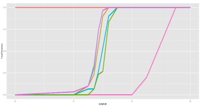
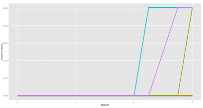
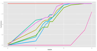
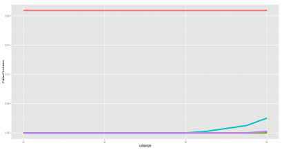
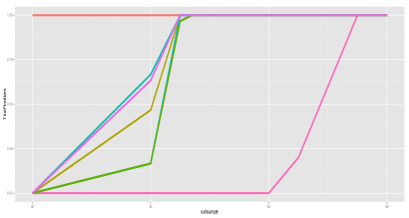
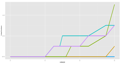
Figure 1: X-axes represents the subsample size $N$ on a logarithmic scale and the Y-axes represents the average selection probability of the signal variables (the first column) and of the noise variables (the second column). The first row is according to Model 1, the second according to Model 2 and the third according to Model 3. Colors represent: red-Lasso, pink-subagging and minimax(6) with brown– $K=1,\tau=1$; dark-brown–$K=1,\tau=1/2$; dark-green–$K=1,\tau=4/5$; green–$K=10,\tau=1$; green-blue–$K=10,\tau=1/2$; light-blue–$K=10,\tau=4/5$; blue–$K=3,\tau=1$ ; purple–$K=3,\tau=1/2$; dark-pink–$K=3,\tau=4/5$.

We complement the results presented in the Figure 1 with the results presented in Tables 1 and 2. There we fix $N=251$ and show average of the true and false positive results for varying choices of the tuning parameter $\lambda_{N}$.

$\lambda_{N}$		$0.001$	$0.005$	$0.008$	$0.01$	$0.03$	0.05	0.1	0.3	0.9	1.5	1.9
Lasso	TP	1	1	1	1	1	1	1	1	1	1	1
	FP	0.94	0.79	0.66	0.59	0.12	0.005	0	0	0	0	0
Subagging	TP	1	1	1	1	1	1	1	1	1	0.93	0.83
	FP	0	0	0	0	0	0	0	0	0	0	0
WMCB, $K=1$, $\tau=1$	TP	1	1	1	1	1	1	1	1	1	0.76	0.46
	FP	0.82	0.01	0.008	0.007	0	0	0	0	0	0	0
WMCB, $K=3$, $\tau=1$	TP	1	1	1	1	1	1	1	1	1	0.90	0.53
	FP	0.99	0.02	0.01	0.01	0	0	0	0	0	0	0
WMCB, $K=10$, $\tau=1$	TP	1	1	1	1	1	1	1	1	1	0.96	0.6
	FP	0.99	0.05	0.02	0.01	0.001	0	0	0	0	0	0
WMCB, $K=1$, $\tau=0.5$	TP	1	1	1	1	1	1	1	1	1	1	0.93
	FP	0.99	0.24	0.20	0.16	0.09	0.07	0.04	0.004	0	0	0
WMCB, $K=3$, $\tau=0.5$	TP	1	1	1	1	1	1	1	1	1	1	1
	FP	0.99	0.47	0.37	0.29	0.13	0.08	0.04	0.003	0	0	0
WMCB, $K=10$, $\tau=0.5$	TP	1	1	1	1	1	1	1	1	1	1	1
	FP	0.99	0.6	0.47	0.36	0.16	0.11	0.06	0.004	0	0	0

Table 1: Average number of true (TP) and false positives (FP) over $100$ replication of a Gaussian linear model with Toeplitz design with $\rho=0.2$ and $\mbox{\boldmath$\beta$}^{*}=(1^{T},0^{T})^{T}$. The model has $p=1000$ and $n=10000$. Subagging and Weighted Maximum-Contrast selection use $N=251$ and $b=3$, $m=3$.

$\lambda_{N}$		$0.001$	$0.005$	$0.008$	$0.01$	$0.03$	0.05	0.1	0.3	0.9	1.5	1.9
Lasso	TP	1	1	1	1	1	1	1	1	1	0	0
	FP	0.88	0.59	0.42	0.29	0.002	0	0	0	0	0	0
Subagging	TP	0.76	0.86	0.86	0.86	0.86	0.86	0.83	0.63	0	0	0
	FP	0	0	0	0	0	0	0	0	0	0	0
WMCB, $K=1$, $\tau=1$	TP	1	1	0.96	0.96	0.96	0.96	0.93	0.4	0	0	0
	FP	0.01	0.003	0.001	0.001	0	0	0	0	0	0	0
WMCB, $K=3$, $\tau=1$	TP	1	1	0.96	0.96	0.96	0.96	0.96	0.46	0	0	0
	FP	0.02	0.001	0	0	0	0	0	0	0	0	0
WMCB, $K=10$, $\tau=1$	TP	1	1	0.97	0.98	0.98	0.99	0.97	0.97	0.97	0.97	0.5
	FP	0.04	0.003	0.002	0.001	0.002	0.001	0	0	0	0	0
WMCB, $K=1$, $\tau=0.5$	TP	1	1	1	1	1	1	1	0.9	0	0	0
	FP	0.25	0.14	0.11	0.12	0.06	0.04	0.003	0.001	0	0	0
WMCB, $K=3$, $\tau=0.5$	TP	1	1	1	1	1	1	1	0.96	0	0	0
	FP	0.46	0.18	0.13	0.13	0.06	0.05	0.01	0	0	0	0
WMCB, $K=10$, $\tau=0.5$	TP	1	1	1	1	1	1	1	1	1	0	0
	FP	0.56	0.22	0.16	0.17	0.08	0.09	0.07	0.02	0	0	0

Table 2: Average number of true (TP) and false positives (FP) over $100$ replication of a Gaussian linear model with Toeplitz design with $\rho=0.2$ and $\mbox{\boldmath$\beta$}^{*}=(0.3^{T},0^{T})^{T}$. The model has $p=1000$ and $n=10000$. Subagging and Weighted Maximum-Contrast selection use $N=251$ and $b=3$, $m=3$.

4.2 Skewed Linear Model

In the next example, we consider two settings that depart from simple dependency and normality assumptions. We consider the same simple linear model as above. Parameter choices are made by the same choices as in the Models 1-3 above: $n=10000$, $p=4000$.

We consider three additional models:

• Model 4: The design matrix has a multivariate Student distribution, with the covariance matrix $\Sigma$ from the Model 3 above. $\mbox{\boldmath$\beta$}^{*}$ is a sparse vector in which the first $30$ elements are equal to $3$ and the rest are equal to $0$. The $\varepsilon_{i}$s are generated as independent, standard Gaussian components.

• Model 5: The design matrix is such that, $X_{ij}$’s are drawn from the Beta distribution with parameters $1+10\frac{j-1}{p-1}$ and $2$ independently for $j=1,\dots,p$. The regression model is calibrated to have mean zero, but the distribution of $\mbox{\bf X}_{i}$ is skewed with skewness that varies across dimensions. $\mbox{\boldmath$\beta$}^{*}$ is a sparse vector in which the first $10$ elements are equal to $1,2,3,\dots,10$ and the rest are equal to $0$. The $\varepsilon_{i}$s are generated as independent, standard Gaussian components.

• Model 6: The design matrix is such that each $\mathbf{X}_{i}$ has a multivariate normal distribution independently, with the covariance matrix $\Sigma$. $\Sigma$ is the covariance matrix of a fractional white noise process, where the difference parameter $l=0.2$. In other words, $\Sigma$ has a polynomial off-diagonal decay, $\mbox{\boldmath$\Sigma$}_{ij}=\mathcal{O}(|i-j|^{1-2l})$. $\mbox{\boldmath$\beta$}^{*}$ is a sparse vector in which the first $10$ elements are equal to $1$ and the rest are equal to $0$. The $\varepsilon_{i}$s are generated as independent components with Student $t$ distribution with $3$ degrees of freedom.

Figures 2 shows results for the regression setting under the three above models. The Lasso estimator is no longer the oracle estimator for all the models; it is an oracle just for the Model 4 where we observe same patters as in Models 1-3. Model 5 is particularly difficult, as column correlations depend through dimensionality $p$. Also, the maximum-contrast estimator is better than the Lasso (for example, $0.8$ versus $0.3$, of the average true positive rate in Model 5), which illustrates the advantage of maximum-contrast estimator for correlated or skewed settings. Model 6 is a challenging model, and we observe that the Lasso estimator fails to recover the correct set of variables. Nevertheless, the maximum-contrast estimator achieves a perfect recovery for all subsample larger than $\sqrt{n}=100$, which illustrates the additional advantage of maximum-contrast estimator for correlated designs. Additionally, note that weight vector $\mathbf{w}_{k}$ is improving the estimation and convergence rate of the introduced method, as the subagging estimators underperform in all of the Models 4-6.

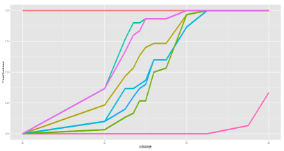
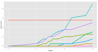
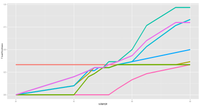
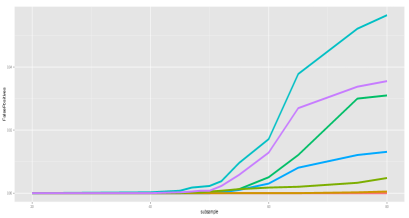
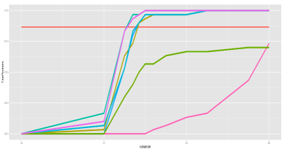
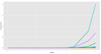
Figure 2: X-axes represents the subsample size $N$ on a logarithmic scale and the Y-axes represents the average selection probability of the signal variables (the first column) and of the noise variables (the second column). The first row is according to Model 4, the second according to Model 5 and the third according to Model 6. Colors represent: red-Lasso, pink-subagging and minimax(6) with brown– $K=1,\tau=1$; dark-brown–$K=1,\tau=1/2$; dark-green–$K=1,\tau=4/5$; green–$K=10,\tau=1$; green-blue–$K=10,\tau=1/2$; light-blue–$K=10,\tau=4/5$; blue–$K=3,\tau=1$ ; purple–$K=3,\tau=1/2$; dark-pink–$K=3,\tau=4/5$.

4.3 Mean Squared Error

Under the same set of Models 1-6 , we investigate the convergence of the proposed method with respect to its mean squared error, as the subsample size $N$ gets larger and larger. In this case, we keep the sample size $n$ to be $10000$. Results are summarized in the Figure 3. The maximum-contrast estimator exhibits faster convergence rate in comparison to the traditional subagging by a large margin across all Models 1-6. Moreover, we see that different choices of $\tau$ do not alter the performance of the estimator by much.

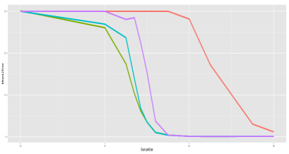
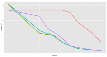
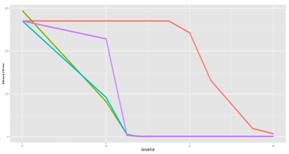
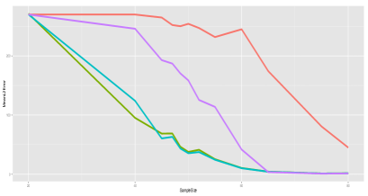
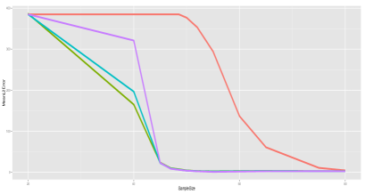
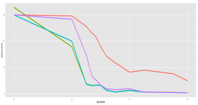
Figure 3: X-axes represents the sample size and the Y-axes represents the average $l_{2}$ error. Simulation settings: the first row is according to Model 1 and 2, the second according to Model 3 and 4, and the third according to Model 5 and 6 . Colors represent: red-subagging and (6) with dark green-$K=3,\tau=0.3$, blue-$K=3,\tau=0.5$ and purple-$K=3,\tau=0.8$

4.4 Sensitivity with respect to the number of blocks $b$

We also test the sensitivity of the proposed method with respect to the choice of the number of blocks $b$. For that purpose, we generate synthetic data from the simple linear model. Model specifications are equivalent to the ones of Model 1. As a measure of performance, we contrast mean selection frequency of the first 30 important variables with a different number of block i.e. boostrap replications. Figure 4 summarizes our findings and reports average selection frequency and its 95% confidence interval for 4 different bootstrap replications: $b=1,2,5$ and $10$. As expected, the larger the $b$, the smaller is the variability in estimating. Interestingly, $b=2$ was sufficient to guarantee perfect recovery for all $\tau>1/2$. Even for $b=1$ this seems to be true in the example considered, but the variability is significantly larger then for $b\geq 2$, hence making general conclusion seem inappropriate.

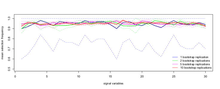
Figure 4: Variability of selection probabilities $\pi_{j}^{*}$ among signal variables with a change in the number of data perturbations ($B=1$, $B=2$,$B=5$ blue, green and pink respectively). X-axes enumerates the first 30 signal variables, whereas the Y-axes show the median selection probability. Dashed lines represent corresponding 95% confidence intervals of it.

5 Discussion

In this paper, we presented results demonstrating that our decomposition-based method for approximate variable selection achieves minimax optimal convergence rates, whenever the number of data partitions is not too large. We allow the number of partitions to grow polynomially with the subsample size. The error guarantees of the maximum-contrast estimator depend on the effective number of blocks of sample splits and the effective dimensionality of the support set (recall bound (14) of Theorem 3). For any number of blocks of sample splits $b\leq\exp\{(1-1/m)n/s+\log n/s\}/2$ and $K\leq\max\{N\rho_{n}^{2}\sqrt{b}/s,Np/s\}$, our method achieves approximate support recovery i.e.

$$P(S\subseteq\hat{S}_{\tau})\geq 1-p^{1-c_{N}},\qquad E|S^{c}\cap\hat{S}_{\tau}|\sim\frac{1}{\sqrt{b}}\frac{s}{p},$$

for all $\lambda_{N}\sqrt{n/\log p}\in(1/c_{N},c_{N})$ and $c_{N}\geq 1$. Theorem 4 confirms these to be minimax optimal for approximate recovery. In addition, we achieve substantial computational benefits coming from the subsampling schemes, in that computational costs scale linearly with $N$ rather than $n$.

The maximal-contrast estimator also has deep connections with the literature of stability selection. Stability selection (Meinshausen and Bühlmann, 2010) and paired stability selection (Shah and Samworth, 2013), and more recent median selection (Wang et al., 2014) can be equivalently formulated as voting estimators. First, we clarify that even when $K=1,m=1,b=d$, maximum-contrast is not the same procedure as Stability selection, although they share the same population objective. The difference is that maximum-contrast utilizes a minimax estimator of the population objective. Second, maximum-contrast is designed for the settings with a growing number of subsamples of a very small size; none of the aforementioned methods can be directly implemented. These methods need a fix number of large subsamples. Third, our theoretical analysis differs from that in the existing work; we do not require irrepresentable condition and we show optimality of the proposed method.

6 Preliminary Lemmas

Let us introduce notation used throughout the proofs. We use $\langle\cdot,\cdot\rangle_{n}$ to denote the empirical inner product, i.e. $\langle\mbox{\bf u},\mbox{\bf v}\rangle_{n}=\frac{1}{n}\mbox{\bf u}^{T}\mbox{\bf v}$. Whenever possible, we will suppress $\lambda_{n}$ and $\lambda_{N}$ in the notation of $\hat{}\mbox{\boldmath$\beta$}(\lambda_{n})$ and $\hat{}\mbox{\boldmath$\beta$}_{i:k}(\lambda_{N})$, and use $\hat{}\mbox{\boldmath$\beta$}$ and $\hat{}\mbox{\boldmath$\beta$}_{i:k}$. Let $P$ and $\mathbb{P}^{*}$ stand for the probability measures generated by the error vector $(\varepsilon_{1},\cdots,\varepsilon_{n})$ and generated jointly by the weights $w_{1},\cdots,w_{N}$ and the errors $\varepsilon_{1},\cdots,\varepsilon_{n}$.

In order to study statistical properties of the proposed estimator, it is useful to present the optimality conditions for solutions of the problems (9) and (3).

$\hat{}\mbox{\boldmath$\beta$}$ is a solution to (9), if and only if

$$\left\langle\mbox{\bf X}_{j},\mbox{\bf Y}-\mbox{\bf X}\hat{}\mbox{\boldmath$\beta$}\right\rangle_{n} =\lambda_{n}\mbox{sign}(\hat{\beta}_{j}), \qquad\hat{\beta}_{j}\neq 0$$ if (16)

$$\left|\left\langle\mbox{\bf X}_{j},\mbox{\bf Y}-\mbox{\bf X}\hat{}\mbox{\boldmath$\beta$}\right\rangle_{n}\right| \leq\lambda_{n}, \qquad\hat{\beta}_{j}=0.$$ if (17)

$\hat{}\mbox{\boldmath$\beta$}_{i:k}$ is a solution to (3), if and only if

$$\left\langle\mbox{\bf D}_{\sqrt{\mathbf{w}_{k}}}\mbox{\bf X}_{I_{i},j},\mbox{\bf D}_{\sqrt{\mathbf{w}_{k}}}\mathbf{Y}_{I_{i}}-\mbox{\bf D}_{\sqrt{\mathbf{w}_{k}}}\mathbf{X}_{I_{i}}\hat{}\mbox{\boldmath$\beta$}_{i:k}\right\rangle_{n} = \lambda_{N}\mbox{sign}(\hat{\beta}_{i:k,j}), \hat{\beta}_{i:k,j}\neq 0$$ if (18)

$$\left|\left\langle\mbox{\bf D}_{\sqrt{\mathbf{w}_{k}}}\mbox{\bf X}_{I_{i},j},\mbox{\bf D}_{\sqrt{\mathbf{w}_{k}}}\mathbf{Y}_{I_{i}}-\mbox{\bf D}_{\sqrt{\mathbf{w}_{k}}}\mathbf{X}_{I_{i}}\hat{}\mbox{\boldmath$\beta$}_{i:k}\right\rangle_{n}\right| \leq \lambda_{N},\qquad\quad \hat{\beta}_{i:k,j}=0.$$ if (19)

In the display above the set of indices $I_{i}$ corresponds to those which were used for the computation of $\hat{}\mbox{\boldmath$\beta$}_{i:k}$.

Below we define the new primal dual witness technique to examine when the solution to one optimization problem is also a solution to the other.

Lemma 3.

Suppose $\hat{}\mbox{\boldmath$\beta$}_{i:k}$ is a solution to the subLasso problem, i.e. it satisfies (18) and (19). Then, if

$$\left|\left\langle\mbox{\bf X}_{j},\mbox{\bf Y}_{I_{i}}-\mbox{\bf X}_{I_{i}}\hat{}\mbox{\boldmath$\beta$}_{i:k}\right\rangle_{n}\right|\leq\lambda_{n}-\lambda_{N},\qquad\mbox{for all }j:\hat{\beta}_{i:k,j}=0,$$

then $\hat{\beta}_{i:k,j}$ satisfies (17), that is $\hat{S}_{i}^{c}\subseteq\hat{S}^{c}$.

Lemma 4.

Suppose $\hat{}\mbox{\boldmath$\beta$}$ is a solution to the Lasso problem, i.e. it satisfies (16) and (17). Then, if

$$\left|\left\langle\mbox{\bf X}_{j},\mbox{\bf Y}_{I_{i}}-\mbox{\bf X}_{I_{i}}\hat{}\mbox{\boldmath$\beta$}\right\rangle_{n}\right|\leq\lambda_{N}/n-\lambda_{n},\qquad\mbox{for all }j:\hat{\beta}_{j}=0,$$

then $\hat{\beta}_{j}$ satisfies (19), that is $\hat{S}^{c}\subseteq\hat{S}_{i}^{c}$.

For the purpose of examining condition number of various design matrices, we first establish a bound on the spectral norm of the difference between the inverses of two positive semidefinite matrices. To establish this result we use Theorem III. 2.8 of Bhatia (1997).

Lemma 5.

Let $\mbox{\bf D},\mbox{\bf G}\in\mathbb{R}^{n\times n}$ be two semi-positive definite matrices. Let $\|\cdot\|$ be a matrix norm induced by the vector $l_{\infty}$ norm. Then,

$$\left\|\mbox{\bf D}^{-1}-\mbox{\bf G}^{-1}\right\|^{2}\leq n\left(\frac{1}{\lambda_{\min}(\mbox{\bf D})}+\frac{1}{\lambda_{\min}(\mbox{\bf G})}\right).$$

Next we show that the solution of the Sub-Lasso problem (3) has good predictive properties. Since proof follows the strategy of Bickel et al. (2009), the proof is presented in the supplement for completeness.

Lemma 6.

Let $\|\mathbf{x}^{j}_{I_{i}}\|_{\infty}\leq c_{2}\sqrt{N/\log p}$, for some constant $c_{2}>1$ and all $1\leq j\leq p$. Then, on the event $\mathcal{A}_{q}(\lambda_{N})=\bigcap_{j=1}^{p}\left\{2\frac{1}{n}\sum_{l\in I_{i}}w_{k,l}|\varepsilon_{i}X_{lj}|\leq\lambda_{N}-q\right\}$, for $q<\lambda_{N}$,

(i) There exists a positive number $\mbox{e}_{n}$ such that $\min\bigl{\{}{{n}^{-1/2}\mathbb{E}_{\mathbf{w}}\{\|\tilde{}\mbox{\bf X}\mathbf{v}\|_{2}\}}/{\|\mathbf{v}_{S}\|_{2}}:|S|\leq s,\mathbf{v}\in\mathbb{R}^{p},\bigl{.}$ $\bigl{.}\mathbf{v}\neq 0,\mathbf{v}\in\mathbb{C}(3,S)\bigl{\}}>\mbox{e}_{n}$. Then, for all $m$ and $b$

$$\left\|\mathbf{X}_{I_{i}}(\boldsymbol{\boldsymbol{\beta}}^{*}-\hat{\boldsymbol{\beta}}_{i:k}(\lambda_{N}))\right\|_{2}^{2}\leq\frac{(4\lambda_{N}-q)^{2}sn}{e_{n}^{2}}a_{N}^{2}\mbox{ for }c_{1}\sigma\sqrt{\frac{\log p}{n}}\leq\lambda_{N}\leq c_{2}\sigma\sqrt{\frac{\log p}{N}},$$

for some positive constant $a_{N}$ such that $P(\min_{1\leq l\leq N}w_{l}\geq\mathbb{E}_{\mathbf{w}}\|\sqrt{\mathbf{w}}\|_{\infty}a_{N}^{-1})\to 1$.

(ii) If Condition 3 holds, then

$$\left\|\tilde{}\mbox{\bf X}_{I_{i}}(\boldsymbol{\boldsymbol{\beta}}^{*}-\hat{\boldsymbol{\beta}}_{i:k}(\lambda_{N}))\right\|_{2}^{2}\leq\frac{(4\lambda_{N}-q)^{2}sn}{\zeta_{N}^{2}},\mbox{ for }c_{1}\sigma\sqrt{\frac{\log p}{n}}\leq\lambda_{N}.$$

Lemma 7.

If Condition 3 holds almost surely for $\tilde{\mathbf{X}}$, and $\lambda_{N}\geq c_{1}\sigma\sqrt{\log p/n}$, then $|{\hat{S}}_{i}(\lambda_{N},k)|\leq\hat{s}:=Cs\lambda_{\max}(\tilde{\mathbf{X}}^{T}\tilde{\mathbf{X}})/(n\zeta_{N}^{2})$ with probability $1-p^{1-c}$, $c>1$.

7 Proofs of the Main Results

In this section, we provide detailed proofs of the main theoretical results of the paper. One difficulty with each of the sub-Lasso problems is that there is no automatic mechanism to provide the regularization parameter $\lambda_{N}$. Note that under Conditions 4 and 3, approximating the true support set becomes equivalent to approximating the support set of the Lasso estimator (9). We explore this connection and find values of the tuning parameter $\lambda_{N}$, which allow the sparsity pattern of the sub-Lasso to approximate the one of the Lasso estimator.

7.1 Proof of Theorem 1

With $k$ fixed, and a little abuse of notation, we use $\hat{}\mbox{\boldmath$\beta$}_{i}$ to denote $\hat{}\mbox{\boldmath$\beta$}_{i:k}$ throughout this proof alone. Utilizing Lemma 3, it suffices to show that the event

$$\Omega_{n}=\left\{\left|\left\langle\mbox{\bf X}_{I_{i}^{c},j},\mbox{\bf Y}_{I_{i}^{c}}-\mbox{\bf X}_{I_{i}^{c}}\hat{\mbox{\boldmath$\beta$}}_{i}\right\rangle_{n}\right|\leq\lambda_{n}-\lambda_{N}\right\},\qquad\mbox{for all }j:\hat{\beta}_{i,j}=0,$$

has large probability. In the display above we used notation

$$\frac{1}{n}\sum_{l\notin I_{i}}X_{lj}(Y_{l}-\mbox{\bf X}_{l}\hat{\mbox{\boldmath$\beta$}}_{i}):=\left\langle\mathbf{X}_{I_{i}^{c},j},\mathbf{Y}_{I_{i}^{c}}-\mathbf{X}_{I_{i}^{c}}\hat{\mbox{\boldmath$\beta$}}_{i}\right\rangle_{n}.$$

Let $\hat{S}_{i}$ denote the set of the non-zero coefficients of $\hat{\mbox{\boldmath$\beta$}}_{i}$. Let us denote with $\hat{A}=\hat{S}_{i}\cup S$. Let $P_{\hat{A}}$ be a projection operator into the space spanned by all variables in the set $\hat{A}$, that is

$$P_{\hat{A}}=\mathbf{X}_{I_{i}^{c},\hat{A}}(\mathbf{X}_{I_{i}^{c},\hat{A}}^{T}\mathbf{X}_{I_{i}^{c},\hat{A}})^{-1}\mathbf{X}_{I_{i}^{c},\hat{A}}^{T}.$$

Then, we can split the inner product $\left\langle\mathbf{X}_{I_{i}^{c},j},\mathbf{Y}_{I_{i}^{c}}-\mathbf{X}_{I_{i}^{c}}\hat{\mbox{\boldmath$\beta$}}_{i}\right\rangle_{n}$ into two terms

$$\left\langle\mathbf{X}_{I_{i}^{c},j},(\mathbb{I}-P_{\hat{A}})(\mathbf{Y}_{I_{i}^{c}}-\mathbf{X}_{I_{i}^{c}}\hat{\mbox{\boldmath$\beta$}}_{i})\right\rangle_{n}+\left\langle\mathbf{X}_{I_{i}^{c},j},P_{\hat{A}}(\mathbf{Y}_{I_{i}^{c}}-\mathbf{X}_{I_{i}^{c}}\hat{\mbox{\boldmath$\beta$}}_{i})\right\rangle_{n}.$$

Controlling the size of the set $\Omega_{n}$ is equivalent to upper bounding previous two expressions separately. The second one is more challenging and is presented first.

7.1.1 Step I: Controlling $\left\langle\mathbf{X}_{I_{i}^{c},j},P_{\hat{A}}(\mathbf{Y}_{I_{i}^{c}}-\mathbf{X}_{I_{i}^{c}}\hat{\mbox{\boldmath$\beta$}}_{i})\right\rangle_{n}$

The KKT equations (18) and (19) provide the upper bound

$$\left\langle\mathbf{X}_{I_{i}^{c},j},P_{\hat{A}}(\mathbf{Y}_{I_{i}^{c}}-\mathbf{X}_{I_{i}^{c}}\hat{\mbox{\boldmath$\beta$}}_{i})\right\rangle_{n}\leq\frac{\lambda_{N}}{n}\mathbf{X}_{I_{i}^{c},j}^{T}\mathbf{X}_{I_{i}^{c},\hat{A}}(\mathbf{X}_{I_{i}^{c},\hat{A}}^{T}\mathbf{X}_{I_{i}^{c},\hat{A}})^{-1}(\mbox{sign}\hat{\mbox{\boldmath$\beta$}}_{i}(\lambda_{N})).$$

By Lemma 7, with high probability

$$|\hat{A}|\leq s+Cs\lambda_{\max}(\tilde{\mathbf{X}}^{T}\tilde{\mathbf{X}})/(n\zeta_{N}):=r,$$ (20)

for some nonnegative constant $C$. Hence, $\lambda_{\min}(\mathbf{X}_{\hat{A}}^{T}\mathbf{X}_{\hat{A}})\geq\inf_{|A|=r}\lambda_{\min}(\mathbf{X}_{A}^{T}\mathbf{X}_{A})$, where the last term is strictly positive by the Condition 3 with a constant $a=1$ and a vector $\mbox{\bf v}=(1,\dots,1,0,\dots,0)$, $\mbox{supp}(\mbox{\bf v})=A$. In turn, we see that the matrix $\mathbf{X}_{A}^{T}\mathbf{X}_{A}$ is invertible with high probability.

We split $\frac{\lambda_{N}}{n}\mathbf{X}_{I_{i}^{c},j}^{T}\mathbf{X}_{I_{i}^{c},\hat{A}}(\mathbf{X}_{I_{i}^{c},\hat{A}}^{T}\mathbf{X}_{I_{i}^{c},\hat{A}})^{-1}(\mbox{sign}\hat{\mbox{\boldmath$\beta$}}_{i}(\lambda_{N}))$ into the sum $T_{1}+T_{2}$ with

$$T_{1}=\frac{\lambda_{N}|\hat{A}|}{n}(\mathbf{X}_{\hat{A}}^{T}\mathbf{X}_{\hat{A}})^{-1}\mathbf{X}_{I_{i}^{c},\hat{A}}^{T}\mathbf{X}_{I_{i}^{c},j}\in\mathbb{R}^{|\hat{A}|}$$

and

$$T_{2}=\frac{\lambda_{N}|\hat{A}|}{n}\left[(\mathbf{X}_{I_{i}^{c},\hat{A}}^{T}\mathbf{X}_{I_{i}^{c},\hat{A}})^{-1}-(\mathbf{X}_{\hat{A}}^{T}\mathbf{X}_{\hat{A}})^{-1}\right]\mathbf{X}_{I_{i}^{c},\hat{A}}^{T}\mathbf{X}_{I_{i}^{c},j}\in\mathbb{R}^{|\hat{A}|}.$$

By the Hölder’s inequality, it suffices to bound $\|T_{1}\|_{\infty}$ and $\|T_{2}\|_{\infty}$. We treat the two terms independently. First, by the triangular inequality

$$\|T_{1}\|_{\infty} \leq \frac{\lambda_{N}|\hat{A}|}{n}\left\|(\mathbf{X}_{\hat{A}}^{T}\mathbf{X}_{\hat{A}})^{-1}\left[\mathbf{X}_{I_{i}^{c},\hat{A}}^{T}\mathbf{X}_{I_{i}^{c},j}-\mathbf{X}_{\hat{A}}^{T}\mathbf{X}_{j}\right]\right\|_{\infty}+\frac{\lambda_{N}|\hat{A}|}{n}\left\|(\mathbf{X}_{\hat{A}}^{T}\mathbf{X}_{\hat{A}})^{-1}\mathbf{X}_{\hat{A}}^{T}\mathbf{X}_{j}\right\|_{\infty}$$

$$:= T_{11}+T_{12}.$$

We proceed to bound $T_{11}$ and $T_{12}$ next. Let us first discuss the term $T_{11}$. By consistency of the vector norm $\|\|$ and its corresponding operator norm $\|\|$, Proposition IV.2.4 of Bhatia (1997), guarantees that

$$\|\mbox{\bf M}\mbox{\bf x}\|\leq\|\mbox{\bf M}\|\|\mbox{\bf x}\|,$$

for a matrix M and a vector x. Therefore, for $\mbox{\bf M}=(\mathbf{X}_{\hat{A}}^{T}\mathbf{X}_{\hat{A}})^{-1}$ and $\mbox{\bf x}=\mathbf{X}_{I_{i}^{c},\hat{A}}^{T}\mathbf{X}_{I_{i}^{c},j}-\mathbf{X}_{\hat{A}}^{T}\mathbf{X}_{j}$,

$$\|T_{11}\|_{\infty}\leq\frac{\lambda_{N}r}{n}\left\|(\mathbf{X}_{\hat{A}}^{T}\mathbf{X}_{\hat{A}})^{-1}\right\|\left\|\mathbf{X}_{I_{i}^{c},\hat{A}}^{T}\mathbf{X}_{I_{i}^{c},j}-\mathbf{X}_{\hat{A}}^{T}\mathbf{X}_{j}\right\|_{\infty},$$

with the induced operator normed $\|\cdot\|$ defined as

$$\left\|(\mathbf{X}_{\hat{A}}^{T}\mathbf{X}_{\hat{A}})^{-1}\right\|=\sup_{\mbox{\bf v}\neq 0}\frac{\|(\mathbf{X}_{\hat{A}}^{T}\mathbf{X}_{\hat{A}})^{-1}\mbox{\bf v}\|_{\infty}}{\|\mbox{\bf v}\|_{\infty}}.$$

Let $\mathcal{E}_{n}=\{\hat{A}=\hat{S}_{i}\cup S,|\hat{A}|\leq r:r\geq 0\}$.

On the event $\mathcal{E}_{n}$, we have

$$\left\|(\mathbf{X}_{\hat{A}}^{T}\mathbf{X}_{\hat{A}})^{-1}\right\|\leq\sup_{A:|A|\leq r}\sup_{\mbox{\bf v}\neq 0}\frac{\|(\mathbf{X}_{A}^{T}\mathbf{X}_{A})^{-1}\mbox{\bf v}\|_{\infty}}{\|\mbox{\bf v}\|_{\infty}}=\max_{\|\mbox{\bf v}\|_{\infty}=1,\mbox{\bf v}\neq 0}\sup_{A:|A|\leq r}{\|(\mathbf{X}_{A}^{T}\mathbf{X}_{A})^{-1}\mbox{\bf v}\|_{\infty}}.$$

For a matrix $\mbox{\bf M}\in\mathbb{R}^{r\times r}$, and its operator and Frobenious norm, a simple inequality holds $\|\mbox{\bf M}\|\leq\sqrt{r}\|\mbox{\bf M}\|_{F}=\sqrt{r}\sqrt{\lambda_{\max}(\mbox{\bf M}^{T}\mbox{\bf M})}$ (Bhatia, 1997). Using such inequality, on the event $\mathcal{E}_{n}$ we have

$$\left\|(\mathbf{X}_{\hat{A}}^{T}\mathbf{X}_{\hat{A}})^{-1}\right\|\leq\sqrt{r}\sup_{A:|A|\leq r}\sqrt{\lambda_{\max}\left((\mathbf{X}_{A}^{T}\mathbf{X}_{A})^{-2}\right)}.$$

Furthermore, as $\lambda_{\max}(\mbox{\bf M}^{-1})=\lambda_{\min}^{-1}(\mbox{\bf M})$ (Bhatia, 1997), on $\mathcal{E}_{n}$

$$\left\|(\mathbf{X}_{\hat{A}}^{T}\mathbf{X}_{\hat{A}})^{-1}\right\|\leq\sqrt{r}/\sup_{|A|\leq r}\lambda_{\min}(\mathbf{X}_{A}^{T}\mathbf{X}_{A})\leq\sqrt{r}/\zeta_{N}^{2},$$

where in the last step Condition 3 guarantees $\lambda_{\min}(\mathbf{X}_{A}^{T}\mathbf{X}_{A})\geq\zeta_{N}^{2}$ on the set $\mathcal{E}_{n}$. At the moment, the bound on $\|T_{11}\|_{\infty}$, conditional on the event $\mathcal{E}_{n}$, is as follows

$$\|T_{11}\|_{\infty}\leq\frac{\lambda_{N}r^{2}}{n\zeta_{N}^{2}}\left\|\mathbf{X}_{I_{i}^{c},\hat{A}}^{T}\mathbf{X}_{I_{i}^{c},j}-\mathbf{X}_{\hat{A}}^{T}\mathbf{X}_{j}\right\|_{\infty}.$$ (22)

Now we observe that simple inequality provides

$$\|\mathbf{X}_{\hat{A}}^{T}\mathbf{X}_{j}\|_{\infty}=\max_{q\in\hat{A}}\sum_{i=1}^{n}|X_{iq}X_{ij}|\geq\max_{q\in\hat{A}}\sum_{i\in I_{i}}|X_{iq}X_{ij}|=\|\mathbf{X}_{I_{i}^{c},\hat{A}}^{T}\mathbf{X}_{I_{i}^{c},j}\|_{\infty}.$$ (23)

Combined with the triangular inequality, conditional on the event $\mathcal{E}_{n}$, guarantees that $T_{11}$ is bounded as

$$\|T_{11}\|_{\infty}\leq\frac{2\lambda_{N}r^{2}}{n\zeta_{N}^{2}}\left\|\mathbf{X}_{\hat{A}}^{T}\mathbf{X}_{j}\right\|_{\infty}.$$ (24)

Moreover, the norm inequality $\|\mbox{\bf x}\|_{\infty}\leq\|\mbox{\bf x}\|_{2}$ holds for any vector x. In combination with Lemmas 1 and 7,

$$\|T_{11}\|_{\infty}=\mathcal{O}_{P}\left(\frac{2\lambda_{N}r^{2}}{n\zeta_{N}^{5}}\right).$$ (25)

For the term $T_{12}$, we first observe that $\|\mbox{\bf x}\|_{\infty}\leq\|\mbox{\bf x}\|_{1}$. Second, if we use equation (8) of Lemma 1, and the result of Lemma 7

$$\|T_{12}\|_{\infty}=\mathcal{O}_{P}\left(\frac{\lambda_{N}r^{3/2}}{n\zeta_{N}}\right).$$ (26)

We now discuss the term $T_{2}$. By the the consistency of the operator and the vector norms we have

$$\|T_{2}\|_{\infty}\leq\frac{\lambda_{N}r}{n}\left\|(\mathbf{X}_{I_{i}^{c},\hat{A}}^{T}\mathbf{X}_{I_{i}^{c},\hat{A}})^{-1}-(\mathbf{X}_{\hat{A}}^{T}\mathbf{X}_{\hat{A}})^{-1}\right\|\|\mathbf{X}_{I_{i}^{c},\hat{A}}^{T}\mathbf{X}_{I_{i}^{c},j}\|_{\infty}$$ (27)

where the operator norm above is defined as

$$\left\|(\mathbf{X}_{I_{i}^{c},\hat{A}}^{T}\mathbf{X}_{I_{i}^{c},\hat{A}})^{-1}-(\mathbf{X}_{\hat{A}}^{T}\mathbf{X}_{\hat{A}})^{-1}\right\|=\sup_{\mbox{\bf v}\neq 0}\frac{\left\|\left((\mathbf{X}_{I_{i}^{c},\hat{A}}^{T}\mathbf{X}_{I_{i}^{c},\hat{A}})^{-1}-(\mathbf{X}_{\hat{A}}^{T}\mathbf{X}_{\hat{A}})^{-1}\right)\mbox{\bf v}\right\|_{\infty}}{\|\mbox{\bf v}\|_{\infty}}.$$

We treat each term in (27) separately.

Using $\mbox{\bf G}=\mathbf{X}_{\hat{A}}^{T}\mathbf{X}_{\hat{A}}$ and $\mbox{\bf D}=\mathbf{X}_{I_{i}^{c},\hat{A}}^{T}\mathbf{X}_{I_{i}^{c},\hat{A}}$ in Lemma 5 we have

$$\left\|(\mathbf{X}_{I_{i}^{c},\hat{A}}^{T}\mathbf{X}_{I_{i}^{c},\hat{A}})^{-1}-(\mathbf{X}_{\hat{A}}^{T}\mathbf{X}_{\hat{A}})^{-1}\right\|\leq\sqrt{r}\sqrt{\lambda_{\min}^{-1}(\mathbf{X}_{I_{i}^{c},\hat{A}}^{T}\mathbf{X}_{I_{i}^{c},\hat{A}})+\lambda_{\min}^{-1}(\mathbf{X}_{\hat{A}}^{T}\mathbf{X}_{\hat{A}})}.$$ (28)

Moreover, on the event $\mathcal{E}_{n}$

$$\lambda_{\min}(\mathbf{X}_{I_{i}^{c},\hat{A}}^{T}\mathbf{X}_{I_{i}^{c},\hat{A}})\geq\lambda_{\min}(\mathbf{X}_{\hat{A}}^{T}\mathbf{X}_{\hat{A}})\geq\inf_{|A|=r}\lambda_{\min}(\mathbf{X}_{A}^{T}\mathbf{X}_{A})\geq\zeta_{n}^{2},$$

where the last inequality follows from Condition 3.

Term $\|\mathbf{X}_{I_{i}^{c},\hat{A}}^{T}\mathbf{X}_{I_{i}^{c},j}\|_{\infty}$ is bounded similarly as with the term $T_{1}$. Therefore, we conclude

$$\|T_{2}\|_{\infty}=\mathcal{O}_{P}\left(\frac{\sqrt{2}\lambda_{N}r^{3/2}}{n\zeta_{n}\zeta_{N}^{3}}\right).$$ (29)

7.1.2 Step II: Controlling $\left\langle\mathbf{X}_{I_{i}^{c},j},(\mathbb{I}-P_{\hat{A}})(\mathbf{Y}_{I_{i}^{c}}-\mathbf{X}_{I_{i}^{c}}\hat{\mbox{\boldmath$\beta$}}_{i})\right\rangle_{n}$

By definition of $\hat{A}$ we have $S\subset\hat{A}$ and by Lemma 7 that $|\hat{A}|\leq r$ with high probability. Hence, with $r$ as in (20), the term of interest is upper bounded with

$$\sup_{A:|A|\leq r}\sup_{j\notin A}\left\langle\mathbf{X}_{I_{i}^{c},j},(\mathbb{I}-P_{A})\boldsymbol{\varepsilon}_{I_{i}^{c}}\right\rangle_{n}.$$

Remember $\|\mbox{\bf X}_{j}\|_{2}=1$. Note that for all $j\notin A$, $|\mbox{\bf X}_{j}^{T}P_{A}\boldsymbol{\varepsilon}|\leq\|P_{A}\boldsymbol{\varepsilon}\|_{2}$. Hence, the expression in the above display is then bounded with

$$\max_{j\in\{1,\cdots,p\}}\left\langle\mathbf{X}_{I_{i}^{c},j},\boldsymbol{\varepsilon}_{I_{i}^{c}}\right\rangle_{n}+\sup_{A:|A|\leq r}\frac{1}{n}\|P_{A}\boldsymbol{\varepsilon}_{I_{i}^{c}}\|_{2}.$$ (30)

Observe that $\|\mathbf{X}_{I_{i}^{c},j}\|_{2}\leq 1$, $|I_{i}^{c}|=N-n$ and that $\langle\cdot,\cdot\rangle$ denotes the empirical inner product. Since $\{\varepsilon_{i}\}_{i=1}^{n}$ are i.i.d. with bounded moments, we have by the weighted Bernstein inequality, that there exists a constant $c>0$ such that for a sequence of positive numbers $u_{n}$

$$P\left(\frac{n}{n-N}\max_{j\in\{1,\cdots,p\}}\left|\left\langle\mathbf{X}_{I_{i}^{c},j},\boldsymbol{\varepsilon}_{I_{i}^{c}}\right\rangle_{n}\right|\geq u_{n}\right)$$

$$=P\left(\frac{1}{n-N}\sum_{i\in I_{i}^{c}}\left|X_{i,j}{\varepsilon}_{i}\right|\geq u_{n}\right)\leq\exp\left\{-c\frac{(N-n)^{2}u_{n}^{2}}{8\sigma^{2}}\right\}.$$ (31)

For a choice of $u_{n}=2\sigma\sqrt{\log p/(N-n)}$ the above probability will converge to zero.

We now bound the second term in (30). Lemma 7 implies that, conditional on the event $\mathcal{E}_{n}$

$$\sqrt{(n-N)}\|P_{\hat{A}}\boldsymbol{\varepsilon}_{I_{i}^{c}}\|_{2}/\sigma\leq\sup_{|A|=r}\sqrt{(n-N)}\|P_{A}\boldsymbol{\varepsilon}_{I_{i}^{c}}\|_{2}/\sigma.$$

Furthermore, $\sup_{|A|=r}\sqrt{(n-N)}\|P_{A}\boldsymbol{\varepsilon}_{I_{i}^{c}}\|_{2}/\sigma$ has a $\chi_{r}$ distribution. Hence, tail bounds of the Chi-squared distribution (Lemma 1 of Laurent and Massart (2000)) lead to

$$P\left((n-N)\sup_{A:|A|\leq r}\|P_{A}\boldsymbol{\varepsilon}_{I_{i}^{c}}\|_{2}^{2}\geq\sigma^{2}r{{(1+4\log p)}{}}\right)\leq\exp\{-3/2r\log p\}.$$ (32)

Plugging in (31) and (32) into (30), we obtain

$$\left|\left\langle\mathbf{X}_{I_{i}^{c},j},(\mathbb{I}-P_{\hat{A}})(\mathbf{Y}_{I_{i}^{c}}-\mathbf{X}_{I_{i}^{c}}\hat{\mbox{\boldmath$\beta$}}_{i})\right\rangle_{n}\right|\leq 2\sigma\sqrt{\frac{(n-N)\log p}{n^{2}}}+2\sigma\sqrt{\frac{4r\log p}{n^{2}(n-N)}}$$ (33)

with probability $1-2p^{-c}$.

Combining (25), (26), (29) and (33) we obtain

$$\left|\left\langle\mathbf{X}_{I_{i}^{c},j},\mathbf{Y}_{I_{i}^{c}}-\mathbf{X}_{I_{i}^{c}}\hat{\mbox{\boldmath$\beta$}}_{i}\right\rangle_{n}\right|\leq\frac{2\lambda_{N}r^{2}}{n\zeta_{N}^{5}}+\frac{2\lambda_{N}r^{3/2}}{n\zeta_{N}}+\frac{\sqrt{2}\lambda_{N}r^{3/2}}{n\zeta_{n}\zeta_{N}^{3}}+2\sigma\sqrt{\frac{(n-N)\log p}{n^{2}}}+2\sigma\sqrt{\frac{4r\log p}{n^{2}(n-N)}},$$

with probability of $1-p^{1-c}$, $c\geq 1$.

Moreover, according to Lemma 3 the RHS of the expression above needs to be smaller than $\lambda_{n}-\lambda_{N}$, for the event $\Omega_{n}$ to hold. This leads to the relation of

$$\lambda_{n} \geq \lambda_{N}+\frac{2\lambda_{N}r^{2}}{n\zeta_{N}^{5}}+\frac{2\lambda_{N}r^{3/2}}{n\zeta_{N}}+\frac{\sqrt{2}\lambda_{N}r^{3/2}}{n\zeta_{n}\zeta_{N}^{3}}+2\sigma\sqrt{\frac{(n-N)\log p}{n^{2}}}+2\sigma\sqrt{\frac{4r\log p}{n^{2}(n-N)}},$$

which completes the proof. ∎

7.2 Proof of Theorem 2

We show that the condition of Lemma 4 holds with high probability for the Lasso estimator $\hat{\boldsymbol{\beta}}=\hat{\boldsymbol{\beta}}(\lambda_{n})$. To that end, we define an event

$$\Omega_{n}=\left\{\left|\left\langle\mbox{\bf X}_{I_{i}^{c},j},\mbox{\bf Y}_{I_{i}^{c}}-\mbox{\bf X}_{I_{i}^{c}}\hat{\mbox{\boldmath$\beta$}}\right\rangle_{n}\right|\leq\lambda_{N}/n-\lambda_{n}\right\},\qquad\mbox{for all }j:\hat{\beta}_{j}=0$$

and show that it has a large probability. In the above, we utilized the following notation

$$\frac{1}{n}\sum_{l\notin I_{i}}X_{lj}(Y_{l}-\mbox{\bf X}_{l}\hat{\boldsymbol{\beta}}):=\left\langle\mathbf{X}_{I_{i}^{c},j},\mathbf{Y}_{I_{i}^{c}}-\mathbf{X}_{I_{i}^{c}}\hat{\mbox{\boldmath$\beta$}}\right\rangle_{n}.$$

Let $\hat{S}$ be the set of non-zero coefficients of the Lasso estimator $\hat{\boldsymbol{\beta}}$. Let $P_{\hat{S}}$ be the projection operator into the space spanned by all variables in the set $\hat{S}$. By repeating similar decomposition analysis developed in Theorem 1, $\left\langle\mathbf{X}_{I_{i}^{c},j},\mathbf{Y}_{I_{i}^{c}}-\mathbf{X}_{I_{i}^{c}}\hat{\mbox{\boldmath$\beta$}}\right\rangle_{n}$ is bounded with

$$\left\langle\mathbf{X}_{I_{i}^{c},j},(\mathbb{I}-P_{\hat{S}})(\mathbf{Y}_{I_{i}^{c}}-\mathbf{X}_{I_{i}^{c}}\hat{\mbox{\boldmath$\beta$}})\right\rangle_{n}+\left\langle\mathbf{X}_{I_{i}^{c},j},P_{\hat{S}}(\mathbf{Y}_{I_{i}^{c}}-\mathbf{X}_{I_{i}^{c}}\hat{\mbox{\boldmath$\beta$}})\right\rangle_{n},$$

the proof setup of Step I and II of Theorem 1 extends easily.

Controlling $\left\langle\mathbf{X}_{I_{i}^{c},j},(\mathbb{I}-P_{\hat{S}})(\mathbf{Y}_{I_{i}^{c}}-\mathbf{X}_{I_{i}^{c}}\hat{\mbox{\boldmath$\beta$}})\right\rangle_{n}$ follows by adapting the proof of Theorem 1 to a different projection matrix. This term is upper bounded by utilizing KKT conditions with

$$\frac{\lambda_{n}}{n}\mathbf{X}_{I_{i}^{c},j}^{T}\mathbf{X}_{I_{i}^{c},\hat{S}}(\mathbf{X}_{I_{i}^{c},\hat{S}}^{T}\mathbf{X}_{I_{i}^{c},\hat{S}})^{-1}(\mbox{sign}\hat{\mbox{\boldmath$\beta$}}(\lambda_{n}))$$

Expression above is bounded by

$$\frac{\lambda_{n}}{n}\mathbf{X}_{I_{i}^{c},j}^{T}\mathbf{X}_{I_{i}^{c},\hat{S}}(\mathbf{X}_{\hat{S}}^{T}\mathbf{X}_{\hat{S}})^{-1}(\mbox{sign}\hat{\mbox{\boldmath$\beta$}}(\lambda_{n}))$$ (34)

$$+ \frac{\lambda_{n}|\hat{S}|}{n}\left\|\left[(\mathbf{X}_{I_{i}^{c},\hat{S}}^{T}\mathbf{X}_{I_{i}^{c},\hat{S}})^{-1}-(\mathbf{X}_{\hat{S}}^{T}\mathbf{X}_{\hat{S}})^{-1}\right]\mathbf{X}_{I_{i}^{c},\hat{S}}^{T}\mathbf{X}_{I_{i}^{c},j}\right\|_{\infty}$$

$$:= U_{1}+U_{2}.$$

We proceed to bound $U_{1}$ and $U_{2}$ independently. By Condition 4, the first term, $U_{1}$, can be bounded with

$$\frac{\lambda_{n}}{n}+\frac{\lambda_{n}|\hat{S}|}{n}\left\|(\mathbf{X}_{\hat{S}}^{T}\mathbf{X}_{\hat{S}})^{-1}\left[\mathbf{X}_{I_{i}^{c},j}^{T}\mathbf{X}_{I_{i}^{c},\hat{S}}-\mathbf{X}_{j}^{T}\mathbf{X}_{\hat{S}}\right]\right\|_{\infty}.$$

By the Hölder’s inequality, the expression above is bounded from above by

$$\frac{\lambda_{n}}{n}+\frac{\lambda_{n}|\hat{S}|}{n}\sup_{|A|\leq r}\lambda_{\min}^{-1}\left(\mathbf{X}_{A}^{T}\mathbf{X}_{A}\right)\sup_{|A|\leq r}\sup_{j\notin A}\left\|\mathbf{X}_{I_{i}^{c},A}^{T}\mathbf{X}_{I_{i}^{c},j}-\mathbf{X}_{A}^{T}\mathbf{X}_{j}\right\|_{\infty},$$

where $r$ denotes the size of the set $\hat{S}$. Its size follows from Lemma B.1 of Bickel et al. (2009), i.e.

$$|\hat{S}|\leq C{s\lambda_{\max}\left(\frac{1}{n}\mathbf{X}^{T}\mathbf{X}\right)}/{\zeta_{n}}:=r$$ (35)

with probability approaching 1. Next, by Condition 3 and Lemma 7 we have, $\sup_{|A|\leq r}\lambda_{\min}^{-1}\left(\mathbf{X}_{A}^{T}\mathbf{X}_{A}\right)\leq\frac{1}{\zeta_{n}^{2}}$ and $\left\|\mathbf{X}_{I_{i}^{c},A}^{T}\mathbf{X}_{I_{i}^{c},j}-\mathbf{X}_{A}^{T}\mathbf{X}_{j}\right\|_{\infty}\leq\left\|\mathbf{X}_{I_{i}^{c},A}^{T}\mathbf{X}_{I_{i}^{c},j}-\mathbf{X}_{A}^{T}\mathbf{X}_{j}\right\|_{2}\leq\sqrt{r}/\zeta_{N-n}$, respectively. Combining all of the above,

$$U_{1}=\mathcal{O}_{P}\left(\frac{\lambda_{n}}{n}+\frac{\lambda_{n}r^{3/2}}{n{\zeta_{n}^{2}\zeta_{N-n}}}\right).$$ (36)

Regarding $U_{2}$ we note that (28) still holds with $\hat{S}$ replacing $\hat{A}$. Moreover, Lemma 1 still applies. Hence, we can conclude

$$U_{2}=\mathcal{O}_{P}\left(\frac{\sqrt{2}\lambda_{n}r^{3/2}}{n\zeta_{n}\zeta_{N-n}^{3}}\right).$$ (37)

Controlling $\left\langle\mathbf{X}_{I_{i}^{c},j},P_{\hat{S}}(\mathbf{Y}_{I_{i}^{c}}-\mathbf{X}_{I_{i}^{c}}\hat{\mbox{\boldmath$\beta$}})\right\rangle_{n}$ is done as in Theorem 1. The same steps still apply by noticing that $S\subseteq\hat{S}$ (as Conditions 4 and 3 hold) and that Lemma 1 holds. Hence, we obtain

$$\left|\left\langle\mathbf{X}_{I_{i}^{c},j},(\mathbb{I}-P_{\hat{A}})(\mathbf{Y}_{I_{i}^{c}}-\mathbf{X}_{I_{i}^{c}}\hat{\mbox{\boldmath$\beta$}})\right\rangle_{n}\right|\leq 2\sigma\sqrt{\frac{(n-N)\log p}{n^{2}}}+2\sigma\sqrt{\frac{4r\log p}{n^{2}(n-N)}}$$ (38)

Adding results of (36) and (37) with the one above, we obtain

$$\left|\left\langle\mathbf{X}_{I_{i}^{c},j},\mathbf{Y}_{I_{i}^{c}}-\mathbf{X}_{I_{i}^{c}}\hat{\mbox{\boldmath$\beta$}}\right\rangle_{n}\right| \leq \frac{\lambda_{n}}{n}+\frac{\lambda_{n}r^{3/2}}{n{\zeta_{n}^{2}\zeta_{N-n}}}+\frac{\sqrt{2}\lambda_{n}r^{3/2}}{n\zeta_{n}\zeta_{N-n}^{3}}$$

$$+ 2\sigma\sqrt{\frac{(n-N)\log p}{n^{2}}}+2\sigma\sqrt{\frac{4r\log p}{n^{2}(n-N)}}$$

with probability $1-p^{1-c}$, $c>1$. Note that for all $\lambda_{n}\geq\sigma\sqrt{\log p/n}$, there exists a constant $C^{\prime}>1$, such that $r\leq C{s\lambda_{\max}\left(\frac{1}{n}\mathbf{X}^{T}\mathbf{X}\right)}/{\zeta_{n}}\leq C^{\prime}s$. According to the definition of $\Omega_{n}$ it suffices to have the RHS above bounded with $\frac{\lambda_{N}}{n}-\lambda_{n}$. In turn, this implies

$$\frac{\lambda_{N}}{n} \geq \lambda_{n}+\frac{\lambda_{n}}{n}+\frac{\lambda_{n}C^{\prime 3/2}s^{3/2}}{n{\zeta_{n}^{2}\zeta_{N-n}}}+\frac{\sqrt{2}\lambda_{n}C^{\prime 3/2}s^{3/2}}{n\zeta_{n}\zeta_{N-n}^{3}}+2\sigma\sqrt{\frac{(n-N)\log p}{n^{2}}}+2\sigma\sqrt{\frac{4C^{\prime}s\log p}{n^{2}(n-N)}}.$$

∎

7.3 Proof of Theorem 3

The main ingredient of the proof is based on the intermediary results stated in Theorems 1 and 2. The first part of the statement follows by utilizing Theorem 1 in order to conclude that $S\subseteq\hat{S}_{\tau}$, with probability close to 1. Unfortunately, as conditions of Theorems 2 contradict those of Theorem 1, we cannot easily use their results to conclude the second part of the statement. Therefore, this paper develops and presents a new method for finding the optimal value of the tuning parameter $\lambda_{N}$. It is based on finding the optimal bias-variance tradeoff, where bias is replaced with variable selection error and variance with prediction error. It allows good, but not the best, prediction properties while obtaining desired variable selection properties. We split the proof into two parts. The first bounds the number of false positives, whereas the second finds the optimal choice of $\lambda_{N}$.

7.3.1 Bounding False Positives

Let $\hat{S}_{i}(\lambda_{N})=\cup_{k=1}^{K}\hat{S}_{i}(\lambda_{N},k)$. Assume that the weighted maximal-contrast subbaging procedure is not worse than a random guess (see Theorem 1 of Meinshausen and Bühlmann (2010)), i.e. for

$$|S^{c}|{\mathbb{E}\left[|S\cap\hat{S}_{i}(\lambda_{N})|\right]}{}\geq{|S|}{}{\mathbb{E}}\left[|S^{c}\cap\hat{S}_{i}(\lambda_{N})|\right]$$ (39)

then the expected number of falsely selected variables is bounded by

$${\mathbb{E}}[|S^{c}\cap\hat{S}_{\tau}|]\leq 2\frac{\sqrt{b}}{1+\sqrt{b}}\frac{K^{M}\left(\max_{1\leq k\leq K}{\mathbb{E}}|\hat{S}_{1}(\lambda_{N},k)|\right)^{M}}{p^{M-1}},$$

for all choices of $\tau\geq\frac{1}{2(1+\sqrt{b})}$.

Proof

Define a binary random variable $H_{K}^{\lambda}=1\{j\subseteq\cap_{l=1}^{m}\hat{S}_{mq+1-l}(\lambda_{N})\}$ for all variables $j\subset\{1,\dots,p\}$ with $\hat{S}_{i}(\lambda_{N})=\cup_{k=1}^{K}\hat{S}_{i}(\lambda_{N},k)$ and $q=1,\cdots,b$. Remember that $mb=d$. Then, the selection probability is expressed as a function of simultaneous selection probability

$${\pi}^{*}_{j}(\lambda_{N}) :=\frac{\sqrt{b}}{1+\sqrt{b}}\mathbb{P}^{*}(j\subseteq\cap_{l=1}^{m}\hat{S}_{mq+1-l}(\lambda_{N}))+\frac{1}{2(1+\sqrt{b})}$$

$$=\frac{\sqrt{b}}{1+\sqrt{b}}E(H_{j}^{\lambda}|Z)+\frac{1}{2(1+\sqrt{b})}$$

where the probability $\mathbb{P}^{*}$ denotes probability with respect to the random sample splitting. Here $Z=(X_{1},\dots,X_{n},Y_{1},\dots,Y_{n})$ denotes the whole original sample of size $n$. Then, for $p_{j}^{*}(\lambda_{N})=\mathbb{P}^{*}(j\subseteq\cap_{l=1}^{m}\hat{S}_{mq+1-l}(\lambda_{N}))$, we have

$$P(\pi_{j}^{*}(\lambda_{N})\geq{\tau})=P\biggl{(}p_{j}^{*}(\lambda_{N})\geq\frac{1+\sqrt{b}}{\sqrt{b}}\biggl{(}\tau-\frac{1}{2(1+\sqrt{b})}\biggl{)}\biggl{)}$$

Then,

$$E(H_{j}^{\lambda}|Z) =E({p}^{*}_{j}(\lambda_{N}))=P(H_{K}^{\lambda}=1)$$

$$\leq\prod_{l=1}^{m}P(K\subseteq\hat{S}_{mq+1-l})=P(j\subseteq\hat{S}_{1}(\lambda_{N}))^{m}.$$

Here $\hat{S}_{1}(\lambda_{N})$ denotes $\cup_{k=1}^{K}\hat{S}_{1}(\lambda_{N},k)$. By Markov inequality for exchangeable Bernoulli random variables, we know that

$$P({p}^{*}_{j}(\lambda_{N})\geq\xi)\leq{E({p}^{*}_{j}(\lambda_{N}))}/{\xi}\leq{P(j\subseteq\hat{S}_{1}(\lambda_{N}))^{m}}/{\xi}.$$

By arguments similar to that of Theorem 1 in Meinshausen and Bühlmann (2010), we know that

$$P(j\subseteq\hat{S}_{1}(\lambda_{N}))\leq{E|\hat{S}_{1}(\lambda_{N})|}/{p}\leq{\max_{1\leq k\leq K}KE|\hat{S}_{1}(\lambda_{N},k)|}/{p}.$$

Hence, for a threshold $\tau\geq\frac{1}{2(1+\sqrt{b})}$ we have

$$P(\pi_{j}^{*}(\lambda_{N})\geq{\tau}) \leq \frac{\sqrt{b}{K^{m}(\max_{1\leq k\leq K}E|\hat{S}_{1}(\lambda_{N},k)|)^{m}}}{(1+\sqrt{b})(\tau-\frac{1}{2(1+\sqrt{b})})p^{m}}$$

$$\leq 2\frac{\sqrt{b}}{1+\sqrt{b}}\frac{K^{m}(\max_{1\leq k\leq K}E|\hat{S}_{1}(\lambda_{N},k)|)^{m}}{p^{m}}.$$

Together with $E[|S^{c}\cap\hat{S}_{\tau}|]=\sum_{j\in S^{c}}P(\max_{\lambda_{N}}\pi_{j}^{*}(\lambda_{N})\geq\tau)$, it leads to the

$$E[|S^{c}\cap\hat{S}_{\tau}|]\leq 2\frac{\sqrt{b}}{1+\sqrt{b}}\frac{K^{m}(\max_{1\leq k\leq K}E|\hat{S}_{1}(\lambda_{N},k)|)^{m}}{p^{m-1}}.$$

7.3.2 Optimal choice of $\lambda_{N}$

Next, we show that proposed aggregated sub-Lasso estimators are better than the random guess in the sense of (39). As expected, such property is not achieved for all values of $\lambda_{N}$. By analyzing equation (39) and utilizing results of Theorem 1, we infer that the sequence of $\lambda_{N}$ that achieves control of false positives and allows results of Theorem 1 to hold, is the optimum of the following optimization problem

$$\min q$$

$$s.t. E|{\hat{S}}_{i}(\lambda_{N})|\leq\frac{1}{2}p^{1-1/m}$$

$$P(\mathcal{A}_{q}(\lambda_{N}))\geq 1-\delta$$

$$\lambda_{N}>0,q\geq 0,\delta>0$$

where the events

$$\mathcal{A}_{q}(\lambda_{N})=\bigcap_{j=1}^{p}\left\{2\frac{1}{n}\sum_{l\in I_{i}}w_{k,l}|\varepsilon_{i}X_{lj}|\leq\lambda_{N}+q\right\}.$$

Although the problem (7.3.2) is stated in terms of $q$, the paper demonstrates that the optimal value of $q$ leads to the optimal value of $\lambda_{N}$.

We provide a few comments on the optimization problem (7.3.2). While allowing deviations of the IR$(N)$ conditions, the first constraint is sufficient to guarantee that sub-Lasso estimators are better than random guessing (i.e. that (39) is satisfied). The second constraint restricts our attention to a sequence of random coverage sets $\mathcal{A}_{q}(\lambda_{N})$. They control variable selection properties, whereas the first constraint intrinsically controls predictive properties. Hence, they cannot be satisfied simultaneously on sets $\mathcal{A}_{0}(\lambda_{N})$. For $q=0$ the best prediction is still achievable, but variable selection is not. Hence, we need to allow for possible deviation of the smallest sets $\mathcal{A}_{0}(\lambda_{N})$ by allowing small perturbations of size $q$. Our goal is to find the smallest possible perturbation $q$, which allows high probability bounds on the selection of the false negatives and simultaneously controls the size of the selected sets in Sub-Lasso estimators.

We further represent conditions of the stochastic problem (7.3.2) in a concise way. Note that from KKT conditions of each of the sub-Lasso problems and definition of the sets $\mathcal{A}_{q}$, we can see that for all $j$ such that $\hat{\beta}_{i:k,j}(\lambda_{N})\neq 0$

$$\frac{1}{n}\sum_{l\in I_{i}}w_{k,l}|\left[\tilde{Y}_{l}-\tilde{}\mbox{\bf X}_{l}\hat{\boldsymbol{\beta}}_{i:k}(\lambda_{N})\right]X_{lj}|={\lambda_{N}}\mbox{sign}(\hat{\beta}_{i:k,j}(\lambda_{N})).$$

Moreover, triangle inequality upper bounds the LHS with

$$\frac{1}{n}\sum_{l\in I_{i}}w_{k,l}|\left[\tilde{}\mbox{\bf X}_{l}\mbox{\boldmath$\beta$}^{*}-\tilde{}\mbox{\bf X}_{l}\hat{\boldsymbol{\beta}}_{i:k}(\lambda_{N})\right]X_{lj}|+\frac{1}{n}\sum_{l\in I_{i}}|w_{k,l}X_{lj}\varepsilon_{l}|.$$

On the set $\mathcal{A}_{q}(\lambda_{N})$ we have that the last term is bounded with $(\lambda_{N}+q)/2$. This leads to

$$\frac{1}{n}\sum_{l\in I_{i}}w_{k,l}\left\|\left[\tilde{}\mbox{\bf X}_{l}\mbox{\boldmath$\beta$}^{*}-\tilde{}\mbox{\bf X}_{l}\hat{\boldsymbol{\beta}}_{i:k}(\lambda_{N})\right]X_{lj}\right\|_{\infty}\geq{\lambda_{N}}-\frac{\lambda_{N}+q}{2}.$$ (41)

Then, on the event $\mathcal{A}_{q}$ from the from the KKT conditions of $\hat{\boldsymbol{\beta}}_{i:k}(\lambda_{N})\neq 0$ for all $j$, such that $\hat{\beta}_{i:k,j}(\lambda_{N})\neq 0$,

$$= \frac{1}{n^{2}}\sum_{j=1}^{p}\left\|{\tilde{}\mbox{\bf X}_{k,j}}^{T}\left(\tilde{}\mbox{\bf X}_{k}\mbox{\boldmath$\beta$}^{*}-\tilde{}\mbox{\bf X}_{k}\hat{\boldsymbol{\beta}}_{i:k}(\lambda_{N})\right)\right\|_{2}^{2}$$

$$\stackrel{{\scriptstyle(i)}}{{\geq}} \frac{1}{n^{2}}\sum_{j\in\hat{S}_{i}(\lambda_{N},k)}\left\|{\tilde{}\mbox{\bf X}_{k,j}}^{T}\left(\tilde{}\mbox{\bf X}_{k}\mbox{\boldmath$\beta$}^{*}-\tilde{}\mbox{\bf X}_{k}\hat{\boldsymbol{\beta}}_{i:k}(\lambda_{N})\right)\right\|_{2}^{2}$$

$$\stackrel{{\scriptstyle(ii)}}{{=}} |{\hat{S}}_{i}(\lambda_{N},k)|(\lambda_{N}-q)^{2}/4,$$

where $(i)$ follows from the non-negativity of the summands and $(ii)$ from (41) and inequality of the vector norms $\|\mbox{\bf x}\|_{\infty}\leq\|\mbox{\bf x}\|_{2}$, for a vector x. All of the above leads to

$$|{\hat{S}}_{i}(\lambda_{N},k)| \stackrel{{\scriptstyle(i)}}{{\leq}} \frac{4\lambda_{\max}({\tilde{\mathbf{X}}_{k}}^{T}\tilde{\mathbf{X}}_{k})}{(\lambda_{N}-q)^{2}n^{2}}\left\|\tilde{\mathbf{X}}_{k}\left[{\boldsymbol{\beta}}^{*}-\hat{\boldsymbol{\beta}}_{i:k}(\lambda_{N})\right]\right\|_{2}^{2},$$ (42)

where inequality $(i)$ follows from the above manipulations and inequality of the norms $\|\mbox{\bf M}^{T}\mbox{\bf x}\|_{2}^{2}\leq\lambda_{\max}(\mbox{\bf M}^{T}\mbox{\bf M})\|\mbox{\bf x}\|_{2}^{2}$ , with a matrix M and a vector x. Moreover, from Lemma 6 (ii) we have that

$$\frac{1}{n}\|\tilde{\mathbf{X}}_{k}({\boldsymbol{\beta}}^{*}-\hat{\boldsymbol{\beta}}_{i:k}(\lambda_{N}))\|_{2}^{2}\leq\frac{(16\lambda_{N}^{2}+q^{2})s}{\zeta_{N}^{2}}.$$

The tower property of expectations together, with (42),

$${\mathbb{E}}|{\hat{S}}_{i}(\lambda_{N})|\leq\frac{(64\lambda_{N}^{2}+4q^{2})sK}{n(\lambda_{N}-q)^{2}\zeta_{N}^{2}}\max_{1\leq k\leq K}\mathbb{E}_{\mathbf{w}}\left(\lambda_{\max}({\tilde{\mathbf{X}}_{k}}^{T}\tilde{\mathbf{X}}_{k})\right).$$ (43)

In the above expressions $\lambda_{N}\geq c_{4}\sqrt{\log p/n}$, for some $c_{4}>0$. We are left to evaluate the size of sets $\mathcal{A}_{q}$. This step of the proof is based on a Bernstein’s inequality for the exchangeable weighted bootstrap sequences contained in an intermediary result Lemma 2. From Lemma 2 we have

$$\mathbb{P}\biggl{(}\Bigl{|}\left\langle\mbox{\boldmath$\varepsilon$}_{I_{i}},\mbox{\bf D}_{\mathbf{w}}\mbox{\bf X}_{I_{i}}\right\rangle_{n}\Bigl{|}>u_{n}\biggl{)}\leq\exp\left\{N\log\mathbf{w}_{2}-\frac{n^{2}u_{n}^{2}}{2\sigma^{2}N\|\mbox{\bf X}_{I_{i}}\|_{\infty,2}+2ncu_{n}\|\mbox{\bf X}_{I_{i}}\|_{\infty,\infty}}\right\},$$

with $\mathbf{w}_{2}$ defined in Condition 1. In display above, $\|\mbox{\bf X}_{I_{i}}\|_{\infty,2}:=\max{}\Bigl{\{}{X}_{I_{i}j}^{2}:I_{i}\subset\{1,\cdots,n\},\Bigl{.}$ $\Bigl{.}|I_{i}|=N,1\leq j\leq p\Bigl{\}}$ and $\|\mbox{\bf X}_{I_{i}}\|_{\infty,\infty}:=\max\Bigl{\{}|{X}|_{I_{i}j}:I_{i}\subset\{1,\cdots,n\},|I_{i}|=N,1\leq j\leq p\Bigl{\}}$. Hence, for $u_{n}=t\sigma\sqrt{2}$, and $t$ such that for two constants $c_{5}$ and $c_{6}$

$$c_{6}\sqrt{\log p/N}\geq t\geq c_{5}\sqrt{\log p/n}$$ (44)

and $\|\mbox{\bf X}_{I_{i}}\|_{\infty,\infty}\leq c_{6}\sqrt{N/\log p\ }$ then there exists a positive constant $c_{0}>1$

$$P\left(\frac{1}{n}\bigl{|}\sum_{l\in I_{i}}w_{k,l}X_{lj}\varepsilon_{l}\bigl{|}>{t}\sigma\sqrt{2}\right)\leq 2\exp\left\{-c_{0}\frac{nt^{2}}{\|\mbox{\bf X}_{I_{i}}\|_{\infty,2}}\right\}.$$

In particular, any choice of $c_{5}<1<c_{6}$ would work; even those as large as $c_{5}=N/n$, $c_{6}=n$ satisfy previous constraints. For a choice of $t$ of $\lambda_{N}-q$ we then have

$$P(\mathcal{A}_{q}(\lambda_{N}))\geq 1-2\exp\left\{-cn(\lambda_{N}-q)^{2}/\|\mbox{\bf X}_{I_{i}}\|_{\infty,2}\right\}\to 1,$$ (45)

as long as $\log\mathbf{w}_{2}^{N}<n/N\log p$, which in turn is guaranteed by the Condition 1.

Now with (43), (44) and (45) we can represent the solution to the stochastic optimization problem (7.3.2) as a solution to the following program

$$\min q\geq 0$$

$$s.t. \frac{(\lambda_{N}-q)^{2}}{\lambda_{N}^{2}+q^{2}/4}\geq{\frac{16sp^{1/m}}{N\zeta_{N}^{2}p}}\max_{1\leq k\leq K}\mathbb{E}_{\mathbf{w}}\left(\lambda_{\max}({\tilde{\mathbf{X}}_{k}}^{T}\tilde{\mathbf{X}}_{k})\right),$$

$$P(\mathcal{A}_{q}(\lambda_{N}))\geq 1-2\exp\left\{-cn(\lambda_{N}-q)^{2}/\|\mbox{\bf X}_{I_{i}}\|_{\infty,2}\right\}$$

$$\max\{c_{4},c_{5}\}\sigma\sqrt{\frac{\log p}{n}}<\lambda_{N}\leq c_{6}\sigma\sqrt{\frac{\log p}{N}}.$$

for constants $\max\{c_{4},c_{5}\}<c_{6}$. The RHS of the last constraint inequality is a consequence of Lemma 6 (which is used numerous times in the steps of the proof). The first constraint of the above problem can be reformulated as

$$\lambda_{N}^{2}>q^{2}+{32q^{2}{\frac{sp^{1/m}}{N\zeta_{N}^{2}p}}}\Lambda_{K}\left({1-\frac{16sp^{1/m}}{N\zeta_{N}^{2}p}}\Lambda_{K}\right)^{-1},$$

with $\Lambda_{K}=\max_{1\leq k\leq K}\mathbb{E}_{\mathbf{w}}\left(\lambda_{\max}({\tilde{\mathbf{X}}_{k}}^{T}\tilde{\mathbf{X}}_{k})\right)$. Then we can see that the optimal values of $q$ are of the order of $c_{7}\sigma\sqrt{\frac{\log p}{n}}$ for a constant $c_{7}>0$ that satisfies

$$c_{7}\leq\sqrt{\frac{n-N}{n}}\frac{\sqrt{\zeta_{N}}+2\sqrt{\Lambda_{K}}}{2\sqrt{\zeta_{N}}+\sqrt{\zeta_{N}}/\lambda_{\min}(\mbox{\bf X}_{I_{i}^{c}}^{T}\mbox{\bf X}_{I_{i}^{c}})}.$$

Notice that the optimal value of $q$ allows sets $\mathcal{A}_{q}(\lambda_{N})$ to have large coverage probability. $c_{4},c_{5},c_{6}$ and $c_{7}$ are constants; they satisfy $0<\max\{c_{4},c_{5}\}+c_{7}<c_{6}$. They are not close , as there is a great deal of latitude as to which number once can choose. For example, constant $c_{6}$ can be chosen to be $\max\{c_{4},c_{5}\}+1$ as constant $c_{7}\leq 1$. All of the above results in the choice of the optimal value of the tuning parameter $\lambda_{N}$ as follows $c_{8}\sigma\sqrt{\frac{\log p}{n}}\leq\lambda_{N}\leq c_{9}\sigma\sqrt{\frac{\log p}{n}}$, where $c_{8}=\max\{c_{1},c_{4},c_{5}\}\leq 1$ and $c_{9}=\min\{c_{2},(c_{6}-c_{7})\}>1$.

∎

7.4 Proof of Theorem 4

7.4.1 Part(a)

To prove the part (a), we use the standard technique of Fanno’s lemma in order to reduce the minimax bound to one problem of testing $M+1$ hypothesis. We split $p$ covariates into $M\geq s$ disjoint subsets $J_{1},\dots,J_{M}$, each of size $p/M$. Let ${J}_{l}$ be a collection of disjoint sets each of sparsity $s$, which we denote with $\{\mathcal{J}_{l}\}$. Hence, each subset $J_{l}$ is a collection of ${p/M\choose s}$, $s$-sparse sets. We proceed by defining probability measures $\mu_{l}$ on the $\mathbb{B}_{0}(s)$ ball to be Dirac measures at $\mbox{\boldmath$\beta$}_{l}$ where $\mbox{\boldmath$\beta$}_{l}$ is chosen as follows. We define $\mbox{\boldmath$\beta$}_{l}$ for $l\neq 0$ as linear combination of vectors in $\mathbb{Z}^{p}$

$$\mbox{\boldmath$\beta$}_{l}=\sum_{\mathbf{z}\in\mathbb{Z}^{p}}\theta_{\mathbf{z},l}\mathbf{z},$$

with $\theta_{\mathbf{z},l}=1$ if $\mathbf{z}=(z_{1},\dots,z_{p})=(1\{1\in\mathcal{J}_{l}\},\dots,1\{p\in\mathcal{J}_{l}\})$ and zero otherwise. Obviously, all $\mbox{\boldmath$\beta$}_{l}\in\mathbb{B}_{0}(s)$ and have $\mathcal{J}_{l}$ as sparsity pattern. These measures $\mu_{l}$ are chosen in such a way that for each $l\geq 1$ there exists a set $\mathcal{J}_{l}$ of cardinality $s$ such that $\mu_{l}\{S\subseteq\mathcal{J}_{l}\}=1$ and all the sets $\mathcal{J}_{l}$ are distinct. The measure $\mu_{0}$ is the Dirac measure at $0$. Consider these $\mu_{l}$ as priors on $\mathbb{B}_{0}(s)$ ball and define the corresponding posteriors $\mathbb{P}_{0},\dots,\mathbb{P}_{M}$ by $\mathbb{P}_{l}(A)=\int_{\boldsymbol{\beta}\in\mathbb{B}_{0}(s)}P_{\boldsymbol{\beta}}(A)d\mu_{l}(\mbox{\boldmath$\beta$}).$

With this choice of $\mbox{\boldmath$\beta$}_{l}$ we can easily check

$$\mathcal{K}(\mathbb{P}_{\boldsymbol{\beta}_{l}},\mathbb{P}_{0})\leq n\rho_{n},$$ (47)

where $\mathcal{K}$ denotes the Kullback-Leibler divergence between two probability measures and for $\rho_{n}<\infty$ and such that

$$\max\left\{\sum_{l=1}^{n}\frac{E(\mathbf{X}_{l}\mathbf{v})^{2}}{\sqrt{n}\|\mathbf{v}_{S}\|_{2}}:|S|\leq s,\mathbf{v}\in\mathbb{R}^{p},\mathbf{v}\neq 0,\mathbf{v}\in\mathbb{C}(3,S)\right\}<\rho_{n}.$$ (48)

Next, observe that

$$\inf_{J}\sup_{\boldsymbol{\beta}\in\mathbb{B}_{0}(s)}P_{\boldsymbol{\beta}}\left(S\not\subseteq J\right)\geq\inf_{J}\sup_{l=1,\cdots,M}\sup_{\mbox{\boldmath$\beta$}\in\Theta_{l}}P_{\mbox{\boldmath$\beta$}}\left(S\not\subseteq J\right)$$

for $\Theta_{l}=\{\mbox{\boldmath$\beta$}:\mbox{supp}(\mbox{\boldmath$\beta$})\subset\mathcal{J}_{l}\}$. By the Scheffe’s theorem and the first Pinsker’s inequality (see Lemma 2.1 and 2.6 of Tsybakov (2009)), the RHS above can be lower bounded with

$$1-\frac{1}{M}\sum_{l=1}^{M}\|\mathbb{P}_{\mbox{\boldmath$\beta$}_{l}}-\mathbb{P}_{0}\|_{TV}\geq 1-\frac{1}{M}\sum_{l=1}^{M}(1-\frac{1}{2}\exp\{-\mathcal{K}(\mathbb{P}_{\boldsymbol{\beta}_{l}},\mathbb{P}_{0})\}),$$

where $\|\|_{TV}$ denotes total variation distance between two probability measures. Notice that we can choose the sets within a collection $\mathcal{J}_{l}$ into ${p/M\choose s}$ ways. Together with (47) we have

$$\inf_{J}\sup_{\boldsymbol{\beta}\in\mathbb{B}_{0}(s)}P_{\boldsymbol{\beta}}\left(S\not\subseteq J\right)\geq\frac{1}{2}\exp\{\log{p/M\choose s}-n\rho_{n}\}\geq\frac{1}{2}\exp\{s^{2}\log(p/s^{2})-n\rho_{n}\}.$$

It suffixes to notice that the RHS is bigger than $p^{1-c^{\prime}}$ under conditions of the theorem.

7.4.2 Part(b)

To prove part (b), we use the Assouad’s lemma with appropriately chosen hypothesis to reduce the minimax bound to $Q$ problems of testing only $2$ hypothesis. Consider the set of all binary sequences of length $p$ that have exactly $s$ non zero elements,

$$\Omega=\{\omega=(\omega_{1},\dots,\omega_{p}),\omega_{i}\in\{0,1\}:\|\omega\|_{0}=s\}.$$

Note that the cardinality of this set is $|\Omega|=2^{s}{p\choose s}$. Let $\rho(\omega,\omega^{\prime})$ be the Hamming distance between $\omega$ and $\omega^{\prime}$, that is $\rho(\omega,\omega^{\prime})=\sum_{q=1}^{Q}1\{\omega_{q}\neq\omega^{\prime}_{q}\}$. First, the focus is on accessing the cardinality of the set $\{\omega^{\prime}\in\Omega:\rho(\omega,\omega^{\prime})\leq 1\}$. Observe that one can choose a subset of size $1$ where $\omega$ and $\omega^{\prime}$ agree and then choose the other $s-1$ coordinates arbitrarily. Hence, the cardinality is less than $3{p\choose 1}$. Now consider the set $A\subset\Omega$ such that $|A|\leq{p\choose s}/{p\choose 1}\leq{(p-s)}$. The set of elements $\omega\in\Omega$ that are within Hamming distance $1$ of some element of $A$ has cardinality of at most $|A|{3}{p\choose 1}<|\Omega|.$ Therefore, for any such set with cardinality $|A|$, there exists an $\omega\in\Omega$ such that $\rho(\omega,\omega^{\prime})>1$ . The expected number of false positives of an estimator $J$ is given by

$$E_{\omega}|J\setminus S_{\omega}|=\sum_{q=1}^{Q}E_{\omega}d_{q}(J,\omega_{q})$$

with $d_{q}(J,\omega_{q})=\rho(1\{q\in J\},w_{q})$ and $\rho$ as Hamming distance. Define the statistic $\omega^{\prime}_{q}=\arg\min_{t=0,1}d_{q}(J,t)$. Then, by the definition of $\omega^{\prime}_{q}$ we have $d_{q}(\omega_{q}^{\prime},\omega_{q})=|\omega_{q}-\omega^{{}^{\prime}}_{q}|\leq d_{q}(J,\omega_{q}^{\prime})+d_{q}(J,\omega_{q})\leq 2d_{q}(J,\omega_{q})$. Moreover,

$$E_{\omega}|J\setminus S_{\omega}|\geq\frac{1}{2}\sum_{q=1}^{p}E_{\omega}|\omega^{\prime}_{q}-\omega_{q}|=\frac{1}{2}E_{\omega}\rho(\omega^{\prime},\omega).$$

Therefore, from Assouad’s Lemma (see Theorem 2.12 of Tsybakov (2009)) we have

$$\inf_{J}\sup_{\boldsymbol{\beta}\in\mathbb{B}_{0}(s)}E_{\boldsymbol{\beta}}|S^{c}\cap J|\geq\frac{1}{2}\inf_{\omega^{\prime}}\sup_{\omega\in\Omega}E_{\omega}\rho(\omega^{\prime},\omega)$$

$$\geq\frac{1}{4}2^{s}{p\choose s}\max\left\{\exp\{-\alpha\},(1-\sqrt{\alpha/2})\right\}$$

as long as $\mathcal{K}(\mathbb{P}_{\omega^{\prime}},\mathbb{P}_{\omega})\leq\alpha<\infty.$ Straight forward computation shows that $\mathcal{K}(P_{\omega^{\prime}},P_{\omega})\leq n\rho_{n}$.

∎

7.5 Proof of Theorem 5

Proof follows simple computations using result of Theorem 1 and equations (10) and (11).

The risk of the estimator $\pi^{*}(\lambda_{n})$ is equal to $E(\pi^{*}(\lambda_{n})-p_{j})^{2}=\frac{1}{4}\frac{1}{(1+\sqrt{b})^{2}}.$ Moreover,

$$\mbox{var}\left(\pi_{j}^{*}(\lambda_{n})\right) \leq \frac{1}{4}\frac{1}{(1+\sqrt{b})^{2}}$$

$$\stackrel{{\scriptstyle(i)}}{{<}} \frac{p_{j}(1-p_{j})}{b}$$

$$\stackrel{{\scriptstyle(ii)}}{{\leq}} \frac{P(\hat{\beta}_{j}(\lambda_{n})\neq 0)\left(1-P(\hat{\beta}_{j}(\lambda_{n})\neq 0)\right)}{b}$$

$$= \mbox{var}\left(\pi_{j}(\lambda_{n})\right)$$

where $(i)$ holds for all $p_{j}\in(1/2-c_{n},1/2+c_{n})$ and for small values of $b$, $c_{n}\sim 1/2$ and $(ii)$ follows from Theorem 1 and equations (10) and (11). ∎

7.6 Proof of Theorem 6

Lemmas 3 and 4 are stated for general sub-Lasso estimator and can easily be adapted to case of bagged estimator. With their help and results of Theorems 1 and 2, we are ready to finalize the proof of Theorem 6. Equivalent of Lemma 3 requires $|\sum_{l\notin I_{i}}(Y_{l}-\mathbf{X}_{l}^{T}\hat{\boldsymbol{\beta}}^{b}(\lambda_{n}^{1}))X_{lj}|\leq n\lambda_{n}-n\lambda_{n}^{1}$ to hold, whereas equivalent of Lemma 4 requires $|\sum_{l\notin I_{i}}(Y_{l}-\mathbf{X}_{l}\hat{\boldsymbol{\beta}}(\lambda_{n})X_{lj}|\leq{\lambda_{n}^{1}}/n-n\lambda_{n}$ to hold. The proof follows easily as a consequence of results obtained in Theorems 3, 1 and 2.

Approximating sparse recovery is not possible as a consequence of the proof of Theorem 3. For the bagged estimator (15), there exists no feasible $q$ that is different from zero, which solves the equivalent of (7.3.2). The equivalent of (7.3.2) would require, on one side $q>\sqrt{\log p/N}$ and on the other $q<\sqrt{\log p/n}$. For $N\ll n$ this is not possible as $\sqrt{\log p/N}>\sqrt{\log p/n}$. For a special case of $N=n/k$, only the choice of $k=1$ and fixed, not divergent $s$ and $p$, allows both conditions to be satisfied.

Second, on the subject of the exact sparse recovery, as a consequence of previous equivalent of Lemma 4 and Theorem 1,

$$\lambda_{n}\geq\lambda_{n}^{1}+\frac{2c_{9}\lambda_{n}^{1}s^{2}}{n\zeta_{N}^{5}}+\frac{2c_{10}\lambda_{n}^{1}s^{3/2}}{n\zeta_{N}}+\frac{\sqrt{2}c_{11}\lambda_{n}^{1}s^{3/2}}{n\zeta_{n}\zeta_{N}^{3}}+2\sigma\sqrt{\frac{(n-N)\log p}{n^{2}}}+2\sigma\sqrt{\frac{4r\log p}{n^{2}(n-N)}},$$ (49)

for some universal, positive and bounded constants $c_{9},c_{10},c_{11}$. As a consequence of equivalent of Lemma 3 and Theorem 2 (where a factor of $1/n$ is lost due to the fact that all weights are equal to $1$)

$${\lambda_{n}^{1}}{} \geq \lambda_{n}+\frac{\lambda_{n}}{n}+\frac{c_{12}\lambda_{n}s^{3/2}}{n{\zeta_{n}^{2}\zeta_{N-n}}}+\frac{\sqrt{2}c_{13}\lambda_{n}s^{3/2}}{n\zeta_{n}\zeta_{N-n}^{3}}+2\sigma\sqrt{\frac{(n-N)\log p}{n^{2}}}+2\sigma\sqrt{\frac{4C^{\prime}s\log p}{n^{2}(n-N)}},$$ (50)

for some universal, positive and bounded constants $c_{12},c_{13}$.

If $N\leq n$ then, from the above contradictory conditions one can see that for all fixed $\lambda_{n}$ and all $j\in\hat{S}(\lambda_{n})$, for all $\lambda_{n}^{1}$, $P(j\in\hat{S}_{i}(\lambda_{n}^{1}))=0$. Moreover, we employ the Massart’s Dvoretzky-Kiefer-Wolfowitz inequality to bound the distance between an empirically determined distribution function and the population distribution function. Hence,

$$P\left(\frac{1}{d}\sum_{i=1}^{d}\mathbbm{1}(j\in\hat{S}_{i}(\lambda_{n}^{1}))\leq\frac{1}{2}P(j\in\hat{S}_{1}(\lambda_{n}^{1}))\right)$$

$$\leq P\left(\sup_{\lambda\in(0,\lambda_{n}^{1}]}\sqrt{n}\left|\frac{1}{d}\sum_{i=1}^{d}\mathbbm{1}(j\in\hat{S}_{i}(\lambda_{n}^{1}))-P(j\in\hat{S}_{1}(\lambda_{n}^{1}))\right|\geq\sqrt{d}/2\ P(j\in\hat{S}_{1}(\lambda_{n}^{1}))\right)$$

$$\leq 2e^{-dP(j\in\hat{S}_{1}(\lambda_{n}^{1}))^{2}/2}.$$

As we have shown that for all $\lambda_{n}^{1}$, $P(j\in\hat{S}_{i}(\lambda_{n}^{1}))=0$, it follows that subagged estimator does not have the same sparsity set as the Lasso estimator, i.e.

$$P\left(\exists\lambda_{n}\geq 0,\exists\lambda_{n}^{1}\geq 0:\hat{S}(\lambda_{n})=\hat{S}^{b}(\lambda_{n}^{1})\right)=0.$$

For a special case of $N=n/k$ we see that the only choice of $k=1$ and fixed, not divergent $s$ and $p$ allows equations (49) and (50) to be satisfied up to a constant. That is, there exist two constants $0<c<\infty$ and $0<c_{1}<\infty$ such that for the choice of $\lambda_{n}=c\lambda_{n}^{1}\geq c_{1}n^{-1/2}$ (i.e. result of Bach (2008) only holds for fixed $p$) ∎

7.7 Proof of Theorem 7

If Condition 3 holds on the bootstrapped data matrix, then the result of this Theorem follows by repeating the steps of the proof of Lemma 6 with simplification of no weighting scheme $\mathbf{w}_{k}$, to obtain

$$\sqrt{\sum_{j\in S}|{\hat{\boldsymbol{\beta}}}_{i:k,j}-\boldsymbol{\boldsymbol{\beta}}^{*}_{j}|^{2}}\leq\frac{\left\|X_{I_{i}}(\hat{\boldsymbol{\beta}}_{i:k}(\lambda_{N})-{\boldsymbol{\beta}}^{*})\right\|_{2}}{\zeta_{N}\sqrt{n}}.$$

Following the steps parallel to those in Bickel et al. (2009), one can obtain the predictive bounds of the order of $s\lambda_{N}/\zeta_{N}^{2}$, for $N=n/k$ and $\lambda_{N}\geq 2\sigma\sqrt{2k\log p/n}$. From the classical results on Lasso prediction bounds, we know that optimal $\lambda_{n}\geq 2\sigma\sqrt{2\log p/n}$. The statement of the theorem follows, if we are able to bound the following expression

$$\delta_{n}=\left|\frac{\lambda_{N}}{\zeta_{N}^{2}}-\frac{\lambda_{n}}{\zeta_{n}^{2}}\right|$$

We write $|\zeta_{N}^{2}-\zeta_{n}^{2}|=\zeta_{n}^{2}-\zeta_{N}^{2}=\epsilon_{n}$ for some $\epsilon_{n}\geq 0$. Then for $\lambda_{N}\leq 2\sigma\sqrt{2k\log p/n}$ we have

$$\delta_{n}=\left|\frac{\lambda_{N}}{\zeta_{n}^{2}-\epsilon_{n}}-\frac{\lambda_{n}}{\zeta_{n}^{2}}\right|<\frac{2\sigma\sqrt{\frac{\log p}{n}}}{\zeta_{n}^{2}}\left(\sqrt{k}\frac{1}{1-\frac{\epsilon_{n}}{\zeta_{n}^{2}}}-1\right)$$

now we claim that if $k\leq 4$ then $\sqrt{k}\frac{1}{1-\frac{\epsilon_{n}}{\zeta_{n}^{2}}}-1\leq C$ for some bounded constant $C>1$. This claim is equivalent to claiming that $\frac{1+\epsilon_{n}/\zeta_{n}^{2}}{1-\epsilon_{n}/\zeta_{n}^{2}}\leq C$, that is $\epsilon_{n}/\zeta_{n}^{2}\leq\frac{C-1}{C+1}$. However, from Condition 3 applied on the full data matrix X, we know that $0\leq\epsilon_{n}<\eta\zeta_{n}^{2}$ for some constant $\eta<1$. Hence, constant $C>1$ that satisfies above properties is $(\eta+1)/(1-\eta)$. Therefore, one can conclude that $\delta_{n}\leq\frac{2C\sigma}{\zeta_{n}^{2}}\sqrt{\frac{\log p}{n}}$. ∎

8 Proofs of Lemmas

8.1 Proof of Lemma 1

Proof.

Observe that $\mathbf{X}_{I,A}(\mathbf{X}_{I,A}^{T}\mathbf{X}_{I,A})^{-1}\mathbf{X}_{I,A}^{T}\mathbf{X}_{I,j}$ is a projection of $\mbox{\bf X}_{I,j}$ onto space spanned by the columns of $\mbox{\bf X}_{I,A}$. Moreover, $\|\mbox{\bf X}_{j}\|_{2}^{2}=1$ and

$$1=\sum_{l=1}^{n}X_{lj}^{2}\geq\sum_{l\in I}X_{lj}^{2}=\|\mbox{\bf X}_{I,j}\|_{2}^{2}.$$

Therefore, by the properties of the projection matrices

$$\left\|\mathbf{X}_{I,A}(\mathbf{X}_{I,A}^{T}\mathbf{X}_{I,A})^{-1}\mathbf{X}_{I,A}^{T}\mathbf{X}_{I,j}\right\|_{2}^{2}\leq 1.$$

Moreover, observe that

$$\|\mbox{\bf M}\mbox{\bf x}\|_{2}^{2}=\mbox{\bf x}^{T}\mbox{\bf M}^{T}\mbox{\bf M}\mbox{\bf x}\geq\lambda_{\min}(\mbox{\bf M}^{T}\mbox{\bf M})\|\mbox{\bf x}\|_{2}^{2}.$$

With $\mbox{\bf M}=\mathbf{X}_{I,A}$ and $\mbox{\bf x}=(\mathbf{X}_{I,A}^{T}\mathbf{X}_{I,A})^{-1}\mathbf{X}_{I,A}^{T}\mathbf{X}_{I,j}$,

$$\left\|\mathbf{X}_{I,A}(\mathbf{X}_{I,A}^{T}\mathbf{X}_{I,A})^{-1}\mathbf{X}_{I,A}^{T}\mathbf{X}_{I,j}\right\|_{2}^{2}\geq\lambda_{\min}\left(\mathbf{X}_{I,A}^{T}\mathbf{X}_{I,A}\right)\left\|(\mathbf{X}_{I,A}^{T}\mathbf{X}_{I,A})^{-1}\mathbf{X}_{I,A}^{T}\mathbf{X}_{I,j}\right\|_{2}^{2}.$$

Next, notice that the last two inequalities combined lead to

$$\left\|(\mathbf{X}_{I,A}^{T}\mathbf{X}_{I,A})^{-1}\mathbf{X}_{I,A}^{T}\mathbf{X}_{I,j}\right\|_{2}^{2}\leq 1/\lambda_{\min}\left(\mathbf{X}_{I,A}^{T}\mathbf{X}_{I,A}\right)\leq 1/\zeta_{N}^{2},$$

where in the last step we used Condition 3 with the vector $\mbox{\bf v}=(1,\dots 1,0,\dots,0)^{T}$ and the constant $a=1$ and have made a simple observation $\lambda_{\min}\left(\mathbf{X}_{I,A}^{T}\mathbf{X}_{I,A}\right)\geq\lambda_{\min}\left(\frac{1}{n}\mathbf{X}_{I,A}^{T}\mathbf{X}_{I,A}\right)$. By the inequality of $l_{p}$ norms, $\|\mbox{\bf x}\|_{2}\geq\sqrt{r}\|\mbox{\bf x}\|_{1}$ for all vectors $\mbox{\bf x}\in\mathbb{R}^{r}$,

$$\left\|(\mathbf{X}_{I,A}^{T}\mathbf{X}_{I,A})^{-1}\mathbf{X}_{I,A}^{T}\mathbf{X}_{I,j}\right\|_{1}^{2}\leq r/\zeta_{N}^{2}.$$

In addition, the following holds

$$1/\zeta_{N}^{2}\geq\left\|(\mathbf{X}_{I,A}^{T}\mathbf{X}_{I,A})^{-1}\mathbf{X}_{I,A}^{T}\mathbf{X}_{I,j}\right\|_{2}^{2}\geq\lambda_{\min}\left((\mathbf{X}_{I,A}^{T}\mathbf{X}_{I,A})^{-2}\right)\left\|\mathbf{X}_{I,A}^{T}\mathbf{X}_{I,j}\right\|_{2}^{2},$$

where the last step follows from the observation $\|\mbox{\bf M}\mbox{\bf x}\|_{2}^{2}=\mbox{\bf x}^{T}\mbox{\bf M}^{T}\mbox{\bf M}\mbox{\bf x}\geq\lambda_{\min}(\mbox{\bf M}^{T}\mbox{\bf M})\|\mbox{\bf x}\|_{2}^{2}$, with $\mbox{\bf M}=(\mathbf{X}_{I,A}^{T}\mathbf{X}_{I,A})^{-1}$ and $\mbox{\bf x}=\mathbf{X}_{I,A}^{T}\mathbf{X}_{I,j}$. Moreover, utilizing the bound $\lambda_{\min}(\mbox{\bf A}^{-1})=\lambda_{\min}^{-1}(\mbox{\bf A})$ for any positive semi-definite matrix A,

$$\|\mathbf{X}_{I,A}^{T}\mathbf{X}_{I,j}\|_{2} \leq \lambda_{\min}^{-1}(\mathbf{X}_{I,A}^{T}\mathbf{X}_{I,A})/{\zeta_{N}}\leq\inf_{|A|=r}\lambda_{\min}^{-1}\left(\mathbf{X}_{I,A}^{T}\mathbf{X}_{I,A}\right)/{\zeta_{N}}\leq\zeta_{N}^{-3},$$ (51)

where Condition 3 guarantees $\lambda_{\min}\left(\mathbf{X}_{I,A}^{T}\mathbf{X}_{I,A}\right)\geq\zeta_{N}$ for any $A$, such that $|A|\leq r$. ∎

8.2 Proof of Lemma 2

Proof.

By simple Markov’s inequality we have

$$\mathbb{P}^{*}\left(|\sum_{l\in I_{i}}w_{l}X_{lj}\varepsilon_{l}|>nu_{n}\right)\leq\inf_{q\geq 0}\left\{\exp\{-nqu_{n}\}\mathbb{E}^{*}\exp\{q|\sum_{l\in I_{i}}w_{l}X_{lj}\varepsilon_{l}|\}\right\}.$$ (52)

Observe that Condition 1 implies that random variables $\exp\{w_{l}X_{lj}\varepsilon_{l}\}$ are negatively dependent. Hence the RHS can be upper bounded with

$$\exp\{-nqu_{n}\}\prod_{l\in I_{i}}\mathbb{E}^{*}\exp\{q|w_{l}X_{lj}\varepsilon_{l}|\},$$

for every $q\geq 0$. Let $\mathbf{w}=(w_{1},\dots,w_{N})$ be a vector of exchangeable random variables that satisfy Condition 1.

Let us define $\mathbf{S}$ to be a random permutation over the set of all combinations of $N$ sized subsets of $1,\dots,n$, by requiring that $w_{\mathbf{S}(1)}\geq w_{\mathbf{S}(2)}\geq\cdots\geq w_{\mathbf{S}(N)}$ and if $w_{\mathbf{S}(j)}=w_{\mathbf{S}(j+1)}$ then $\mathbf{S}(j)<\mathbf{S}(j+1)$. This is one possible definition that is unambiguous to the presence of ties. Let $\mathbf{R}$ denote a random permutation uniformly distributed over the set of all combinations of $N$ sized subsets of $1,\dots,n$. Note that $X_{1},\dots,X_{n}$ are independent of $(\mathbf{w},\mathbf{R})$. Observe that $\mathbf{R}$ is independent of $(\mathbf{w},\mathbf{S})$. Notice that $\mathbb{P}=P_{\epsilon}\times P_{w}$. By exchangeability of vector $\mathbf{w}_{k}$, for $l\in I_{i}$ we have

$$\mathbb{E}\exp\{q|w_{l}X_{lj}\varepsilon_{l}|\} =\mathbb{E}_{w}E_{\varepsilon}\exp\{q|w_{l}X_{lj}\varepsilon_{l}|\}=\mathbb{E}_{w}E_{\varepsilon}\exp q|w_{l}X_{\mathbf{R}(l)j}\varepsilon_{\mathbf{R}(l)}|$$

$$=\mathbb{E}_{w}E_{\varepsilon}\exp q|w_{\mathbf{S}(l)}X_{\mathbf{R}\circ\mathbf{S}(l)j}\varepsilon_{\mathbf{R}\circ\mathbf{S}(l)}|.$$

Let $\circ$ denote pointwise multiplication. Observe that $\mathbf{R}\circ\mathbf{S}$ is independent of $\mathbf{S}$ and has the same distribution as R. Therefore, for an $l\in I_{i}$,

$$\mathbb{E}\exp\{|qw_{l}X_{lj}\varepsilon_{l}|\} =\mathbb{E}_{w}\Bigl{[}E_{\varepsilon}\bigl{[}\exp q|w_{\mathbf{S}(l)}X_{\mathbf{R}\circ\mathbf{S}(l)j}\varepsilon_{\mathbf{R}\circ\mathbf{S}(l)}|\bigl{]}\Bigl{]}$$

$$\stackrel{{\scriptstyle(i)}}{{\leq}}\sqrt{\mathbb{E}_{w}\Bigl{[}\exp 2|w_{\mathbf{S}(l)}|\Bigl{]}}\sqrt{E_{\varepsilon}\Bigl{[}\exp 2q|X_{\mathbf{R}(l)j}\varepsilon_{\mathbf{R}\circ\mathbf{S}(l)}|\Bigl{]}}$$

$$\stackrel{{\scriptstyle(ii)}}{{\leq}}\mathbf{w}_{2}\sqrt{E_{\varepsilon}\Bigl{[}\exp 2q|X_{\mathbf{R}(l)j}\varepsilon_{\mathbf{R}(l)}|\Bigl{]}},$$ (53)

where $(i)$ follows from Cauchy Schwarz inequality and $(ii)$ follows from

$$\mathbf{w}_{2}^{2}=\mathbb{E}_{w}\exp 2|w_{\mathbf{S}(l)}|=\int_{0}^{\infty}P_{w}\left(\exp 2|w_{\mathbf{S}(l)}|\geq t\right)dt=\int_{0}^{\infty}P_{w}\left(|w_{\mathbf{S}(l)}|\geq\frac{1}{2}\log t\right)dt.$$

Next, observe that $P_{w}(X_{i}>a)\leq P_{w}(\sup_{i}X_{i}>a)$ holds for any $a\in\mathbb{R}$. Hence,

$$\mathbf{w}_{2}\leq\sqrt{\int_{0}^{\infty}\sup_{l\in I_{i}}P_{w}\left(w_{\mathbf{S}(l)}\geq\frac{1}{2}\log t\right)dt}\leq\sqrt{\int_{0}^{e^{2n}}P_{w}\left(w_{\mathbf{S}(1)}\geq\frac{1}{2}\log t\right)dt}.$$ (54)

where in the last step we observed that $\max_{l\in I_{i}}w_{i}\leq\sum_{l\in I_{i}}w_{l}=n$ by Condition 1.

Furthermore, the Taylor expansion around $0$ provides

$$E_{\varepsilon}\exp q|X_{\mathbf{R}(l)j}\varepsilon_{\mathbf{R}(l)}|=1+E_{\varepsilon}q|X_{\mathbf{R}(l)j}\varepsilon_{\mathbf{R}(l)}|+q^{2}|X_{\mathbf{R}(l)j}|^{2}\sum_{r=2}^{\infty}\frac{1}{r!}|qX_{\mathbf{R}(l)j}|^{r-2}E_{\varepsilon}|\varepsilon_{\mathbf{R}(l)}|^{r}.$$

Since $E_{\varepsilon}[\varepsilon_{i}]=0$ and $E_{\varepsilon}|\varepsilon_{\mathbf{R}(l)}|^{r}\leq r!\sigma^{2}c^{r-2}/2$ we have

$$E_{\varepsilon}\exp q|X_{\mathbf{R}(l)j}\varepsilon_{\mathbf{R}(l)}|\leq 1+\frac{|X_{\mathbf{R}(l)j}|^{2}\sigma^{2}q^{2}}{2}\sum_{r=2}^{\infty}q^{r-2}|X_{\mathbf{R}(l)j}|^{r-2}c^{r-2},$$

for some constant $c<\infty$.

As $\log e^{\lambda x}\leq e^{\lambda x}-1$, for all $q\leq 1/c$, we have the following estimation of logarithmic moment generating function

$$\log E_{\varepsilon}\exp q|X_{\mathbf{R}(l)j}\varepsilon_{\mathbf{R}(l)}|\leq|X_{\mathbf{R}(l)j}|^{2}\sigma^{2}q^{2}\left(1-qc|X_{\mathbf{R}(l)j}|\right)^{-1}.$$

Observe that $|X_{\mathbf{R}(l)j}|\leq\max_{1\leq l\leq N}\|\mbox{\bf X}_{\mathbf{R}(l)}\|_{\infty}\leq\|\mbox{\bf X}_{I_{i}}\|_{\infty,\infty}$. Hence, the logarithmic moment generating function satisfies

$$\log E_{\varepsilon}\exp q|X_{\mathbf{R}(l)j}\varepsilon_{\mathbf{R}(l)}|\leq|X_{\mathbf{R}(l)j}|^{2}\sigma^{2}q^{2}\left(1-qc\|\mbox{\bf X}_{I_{i}}\|_{\infty,\infty}\right)^{-1}.$$ (55)

Utilizing (52) - (55)

$$\mathbb{P}\left(|\sum_{l\in I_{i}}w_{l}X_{lj}\varepsilon_{l}|>nu_{n}\right) \leq e^{N\log\mathbf{w}_{2}}\inf_{q\geq 0}\Biggl{\{}\exp\left\{-nqu_{n}+\frac{\sigma^{2}q^{2}}{2}\sum_{l=1}^{N}|X_{\mathbf{R}(l)j}|^{2}\left(1-qc\|\mbox{\bf X}_{I_{i}}\|_{\infty,\infty}\right)^{-1}\right\}\Biggl{\}}.$$

Since the right hand side above depends on $q$, we proceed to find the optimal $q$ that minimizes it. This is simply done, and the optimal $q$ is

$$q=\frac{nu_{n}}{\sigma^{2}\sum_{l=1}^{N}|X_{\mathbf{R}(l)j}|^{2}+cnu_{n}\|\mbox{\bf X}_{I_{i}}\|_{\infty,\infty}}.$$

This optimal $q$ leads to the bound

$$\mathbb{P}\left(|\sum_{l\in I_{i}}w_{l}X_{lj}\varepsilon_{l}|>nu_{n}\right)\leq{\mathbf{w}_{2}}^{N}\exp\left\{-\frac{n^{2}u_{n}^{2}}{2\sum_{l=1}^{N}|X_{\mathbf{R}(l)j}|^{2}\sigma^{2}+2ncu_{n}\|\mbox{\bf X}_{I_{i}}\|_{\infty,\infty}}\right\}.$$

By observing simple relations $\sum_{l=1}^{N}|X_{\mathbf{R}(l)j}|^{2}=\|X_{\mathbf{R}(l)j}\circ X_{\mathbf{R}(l)j}\|_{1}\leq N\max_{1\leq l\leq N}\max_{1\leq j\leq p}|X_{\mathbf{R}(l)j}|^{2}$, with the last term being upper bounded with $N\|\mbox{\bf X}_{I_{i}}\|_{\infty,2}=N\max_{1\leq j\leq p}|\mbox{\bf X}_{I_{i}j}|^{2}$ we obtain

$$\mathbb{P}\left(|\sum_{l\in I_{i}}w_{l}X_{lj}\varepsilon_{l}|>nu_{n}\right)\leq\exp\left\{N\log\mathbf{w}_{2}-\frac{n^{2}u_{n}^{2}}{2\sigma^{2}N\|\mbox{\bf X}_{I_{i}}\|_{\infty,2}+2ncu_{n}\|\mbox{\bf X}_{I_{i}}\|_{\infty,\infty}}\right\}.$$

∎

8.3 Proof of Lemma 3

Proof.

We want to show that for all $j$ for which $\hat{\boldsymbol{\beta}}_{i:k,j}(\lambda_{N})=0$ and (19) hold, equation (17) also hold, that is

$$\left|\left\langle\mbox{\bf X}_{j},\mbox{\bf Y}-\mbox{\bf X}\hat{}\mbox{\boldmath$\beta$}_{i:k}\right\rangle_{n}\right|\leq\lambda_{n}.$$

As $\mathbf{w}_{k}$ is a vector of a strictly positive random variables, $\min_{1\leq j\leq N}\sqrt{w_{k,j}}<\sum_{j=1}^{N}\sqrt{w_{k,j}}$. Hence, the desired inequality above follows easily from the following inequality

$$\left|\left\langle\mbox{\bf X}_{j},\mbox{\bf Y}-\mbox{\bf X}\hat{}\mbox{\boldmath$\beta$}_{i:k}\right\rangle_{n}\right|\leq\left|\left\langle\mbox{\bf D}_{\sqrt{\mathbf{w}}_{k}}\mbox{\bf X}_{I_{i},j},\mbox{\bf D}_{\sqrt{\mathbf{w}}_{k}}\mbox{\bf Y}_{I_{i}}-\mbox{\bf D}_{\sqrt{\mathbf{w}}_{k}}\mbox{\bf X}_{I_{i}}\hat{}\mbox{\boldmath$\beta$}_{i:k}\right\rangle_{n}\right|+\left|\left\langle\mbox{\bf X}_{I_{i}^{c},j},\mbox{\bf Y}_{I_{i}^{c}}-\mbox{\bf X}_{I_{i}^{c}}\hat{}\mbox{\boldmath$\beta$}_{i:k}\right\rangle_{n}\right|$$

where the first term in the rhs is bounded by $\lambda_{N}$ (by (19)) and the second with $\lambda_{n}-\lambda_{N}$ (by the assumption of the Lemma). ∎

8.4 Proof of Lemma 4

Proof.

Let us assume that for those $j$ such that $\hat{\boldsymbol{\beta}}_{j}=0$, (17) holds. We show that for such $j$’s, equation (19) also holds. First we observe,

$$\left|\left\langle\mbox{\bf X}_{j},\mbox{\bf Y}-\mbox{\bf X}\hat{}\mbox{\boldmath$\beta$}\right\rangle_{n}\right|\geq\left|\left\langle\mbox{\bf X}_{I_{i},j},\mbox{\bf Y}_{I_{i}}-\mbox{\bf X}_{I_{i}}\hat{}\mbox{\boldmath$\beta$}\right\rangle_{n}-\left\langle\mbox{\bf X}_{I_{i}^{c},j},\mbox{\bf Y}_{I_{i}^{c}}-\mbox{\bf X}_{I_{i}^{c}}\hat{}\mbox{\boldmath$\beta$}\right\rangle_{n}\right|$$

By analyzing two cases individually:

Case (I): $\left|\left\langle\mbox{\bf X}_{I_{i},j},\mbox{\bf Y}_{I_{i}}-\mbox{\bf X}_{I_{i}}\hat{}\mbox{\boldmath$\beta$}\right\rangle_{n}\right|\leq\left|\left\langle\mbox{\bf X}_{I_{i}^{c},j},\mbox{\bf Y}_{I_{i}^{c}}-\mbox{\bf X}_{I_{i}^{c}}\hat{}\mbox{\boldmath$\beta$}\right\rangle_{n}\right|$, and

Case (II): $\left|\left\langle\mbox{\bf X}_{I_{i},j},\mbox{\bf Y}_{I_{i}}-\mbox{\bf X}_{I_{i}}\hat{}\mbox{\boldmath$\beta$}\right\rangle_{n}\right|\geq\left|\left\langle\mbox{\bf X}_{I_{i}^{c},j},\mbox{\bf Y}_{I_{i}^{c}}-\mbox{\bf X}_{I_{i}^{c}}\hat{}\mbox{\boldmath$\beta$}\right\rangle_{n}\right|$, we have

$$\left|\left\langle\mbox{\bf X}_{I_{i},j},\mbox{\bf Y}_{I_{i}}-\mbox{\bf X}_{I_{i}}\hat{}\mbox{\boldmath$\beta$}\right\rangle_{n}\right|\leq\left|\left\langle\mbox{\bf X}_{I_{i}^{c},j},\mbox{\bf Y}_{I_{i}^{c}}-\mbox{\bf X}_{I_{i}^{c}}\hat{}\mbox{\boldmath$\beta$}\right\rangle_{n}\right|+\lambda_{n}$$

holds in both cases. With it we can then see that

$$\left|\left\langle\mbox{\bf D}_{\sqrt{\mathbf{w}}_{k}}\mbox{\bf X}_{I_{i},j},\mbox{\bf D}_{\sqrt{\mathbf{w}}_{k}}\mbox{\bf Y}_{I_{i}}-\mbox{\bf D}_{\sqrt{\mathbf{w}}_{k}}\mbox{\bf X}_{I_{i}}\hat{}\mbox{\boldmath$\beta$}\right\rangle_{n}\right|\leq n\left|\left\langle\mbox{\bf X}_{I_{i}^{c},j},\mbox{\bf Y}_{I_{i}^{c}}-\mbox{\bf X}_{I_{i}^{c}}\hat{}\mbox{\boldmath$\beta$}\right\rangle_{n}\right|+n\lambda_{n}$$

since $\|\mbox{\bf D}_{\sqrt{\mathbf{w}}_{k}}^{2}\|_{F}=\|\mbox{\bf D}_{\mathbf{w}_{k}}\|_{F}\leq n$ for all $k$ almost surely. Hence to show that $\hat{\boldsymbol{\beta}}$ satisfies KKT for sub-Lasso as well, we need $\left|\left\langle\mbox{\bf X}_{I_{i}^{c},j},\mbox{\bf Y}_{I_{i}^{c}}-\mbox{\bf X}_{I_{i}^{c}}\hat{}\mbox{\boldmath$\beta$}\right\rangle_{n}\right|\leq\frac{\lambda_{N}}{n}-\lambda_{n}.$ We observe that the last inequality is in the statement of the lemma. ∎

8.5 Proof of Lemma 5

Proof.

Note that by $\|\mbox{\bf D}\|\leq\sqrt{n}\|\mbox{\bf D}\|_{F}$ and the definition of the Frobenius norm we have that for two semi-positive definite matrices $\mbox{\bf D},\mbox{\bf G}\in\mathbb{R}^{n\times n}$

$$\left\|\mbox{\bf D}^{-1}-\mbox{\bf G}^{-1}\right\|=\sqrt{n}\sqrt{\max\biggl{\{}\left|\lambda_{\min}(\mbox{\bf D}^{-1}-\mbox{\bf G}^{-1})\right|,\left|\lambda_{\max}(\mbox{\bf D}^{-1}-\mbox{\bf G}^{-1})\right|\biggl{\}}}.$$

For all $i,j\geq 1$ and $i+j-1\leq n$, Weyls inequalities and Theorem III.2.8 of Bhatia (1997) we have

$$\lambda_{i+j-1}(\mbox{\bf D}+\mbox{\bf G})\leq\lambda_{i}(\mbox{\bf D})+\lambda_{j}(\mbox{\bf G}).$$

Utilizing that $\lambda_{\max}(-\mbox{\bf G}^{-1})=-\lambda_{\min}(\mbox{\bf G}^{-1})=-\lambda_{\min}^{-1}(\mbox{\bf G})$ and $\lambda_{\max}(\mbox{\bf D}^{-1})=\lambda_{\max}^{-1}(\mbox{\bf D})$ we have

$$\lambda_{\max}(\mbox{\bf D}^{-1}-\mbox{\bf G}^{-1})\leq\left|\frac{1}{\lambda_{\max}(\mbox{\bf D})}-\frac{1}{\lambda_{\min}(\mbox{\bf G})}\right|,$$

$$\lambda_{\min}(\mbox{\bf D}^{-1}-\mbox{\bf G}^{-1})\leq\left|\frac{1}{\lambda_{\min}(\mbox{\bf D})}-\frac{1}{\lambda_{\min}(\mbox{\bf G})}\right|.$$

Therefore,

$$\left\|\mbox{\bf D}^{-1}-\mbox{\bf G}^{-1}\right\|\leq\sqrt{n}\sqrt{\left|\frac{1}{\lambda_{\min}(\mbox{\bf D})}-\frac{1}{\lambda_{\min}(\mbox{\bf G})}\right|}\leq\sqrt{n}\sqrt{\frac{1}{\lambda_{\min}(\mbox{\bf D})}+\frac{1}{\lambda_{\min}(\mbox{\bf G})}}.$$

∎

A Supplementary Matterials

A.1 Proof of Lemma 6

Proof.

Note that part (ii) of this Lemma is an easy consequence of Lemma B.1 in Bickel et al. (2009), hence we omit the details. For part(i) we proceed as follows. From the definition, we have for every realization of random weights $\mathbf{w}_{k}$,

$$\frac{1}{n}\sum_{l\in I_{i}}w_{k,l}(Y_{l}-\mbox{\bf X}_{l}\hat{\boldsymbol{\beta}}_{i:k}(\lambda_{N}))^{2}+2\lambda_{N}\|\hat{\boldsymbol{\beta}}_{i:k}(\lambda_{N})\|_{1}\leq\frac{1}{n}\sum_{l\in I_{i}}w_{k,l}(Y_{l}-\mbox{\bf X}_{l}{{\boldsymbol{\beta}}})^{2}+2\lambda_{N}\|\beta\|_{1}$$

holds for any value of $\beta$. For simplicity of the notation we have suppressed the dependence $\hat{\boldsymbol{\beta}}_{i:k}(\lambda_{N})$ of $\lambda_{N}$ and $k$. By using $Y_{i}=X_{l}{\boldsymbol{\beta}}^{*}+\varepsilon_{i}$, and setting $\boldsymbol{\beta}={\boldsymbol{\beta}}^{*}$, previous becomes equivalent to

$$\frac{1}{n}\sum_{l\in I_{i}}w_{k,l}(\mbox{\bf X}_{l}{\boldsymbol{\beta}}^{*}-\mbox{\bf X}_{l}\hat{\boldsymbol{\beta}}_{i:k}(\lambda_{N}))^{2} \leq 2\frac{\|\hat{\boldsymbol{\beta}}_{i:k}(\lambda_{N})-{\boldsymbol{\beta}}^{*}\|_{1}}{n}\max_{1\leq j\leq p}\left(\sum_{l\in I_{i}}w_{k,l}|\varepsilon_{i}X_{lj}|\right)$$

$$+ 2\lambda_{N}\|{\boldsymbol{\beta}}^{*}\|_{1}+2\lambda_{N}\|{\boldsymbol{\beta}}_{i}\|_{1}.$$

Consider the event $\mathcal{A}_{q}(\lambda_{N})=\bigcap_{j=1}^{p}\left\{2\frac{1}{n}\sum_{l\in I_{i}}w_{k,l}|\varepsilon_{i}X_{lj}|\leq\lambda_{N}-q\right\}$, for $q<\lambda_{N}$. Using the fact that $w_{l}\geq 1$ for all $l\in I_{i}$ we have the following

$$\frac{1}{n}\min_{1\leq l\leq N}w_{l}\left\|\mbox{\bf X}_{I_{i}}(\boldsymbol{\boldsymbol{\beta}}^{*}-\hat{\boldsymbol{\beta}}_{i:k}(\lambda_{N}))\right\|_{2}^{2}+\lambda_{N}\|\hat{\boldsymbol{\beta}}_{i:k}(\lambda_{N})-\boldsymbol{\boldsymbol{\beta}}^{*}\|_{1}$$

$$\leq\frac{1}{n}\sum_{l\in I_{i}}w_{l}(\mbox{\bf X}_{l}\boldsymbol{\boldsymbol{\beta}}^{*}-\mbox{\bf X}_{l}\hat{\boldsymbol{\beta}}_{i:k}(\lambda_{N}))^{2}+\lambda_{N}\|\hat{\boldsymbol{\beta}}_{i:k}(\lambda_{N})-\boldsymbol{\boldsymbol{\beta}}^{*}\|_{1}$$

$$\leq(2\lambda_{N}-q)\|\hat{\boldsymbol{\beta}}_{i:k}(\lambda_{N})-\boldsymbol{\boldsymbol{\beta}}^{*}\|_{1}+2\lambda_{N}\|\boldsymbol{\boldsymbol{\beta}}^{*}\|_{1}-2\lambda_{N}\|\hat{\boldsymbol{\beta}}_{i:k}(\lambda_{N})\|_{1}$$

$$\leq(4\lambda_{N}-q)\sum_{j\in S}|{\hat{\boldsymbol{\beta}}}_{i,j}-\boldsymbol{\boldsymbol{\beta}}^{*}_{j}|$$

which leads to the first conclusion. From the previous result

$$\lambda_{N}\|\hat{\boldsymbol{\beta}}_{i:k}(\lambda_{N})-\boldsymbol{\boldsymbol{\beta}}^{*}\|_{1}\leq(4\lambda_{N}-q)\sum_{j\in S}|{\hat{\boldsymbol{\beta}}}_{i,j}-\boldsymbol{\boldsymbol{\beta}}^{*}_{j}|\leq(4\lambda_{N}-q)\sqrt{s}\sqrt{\sum_{j\in S}|{\hat{\boldsymbol{\beta}}}_{i,j}-\boldsymbol{\boldsymbol{\beta}}^{*}_{j}|^{2}}$$

leading to $\hat{\boldsymbol{\beta}}_{i:k}(\lambda_{N})-{\boldsymbol{\beta}}^{*}\in\mathbb{C}(3,S)$. Using the Expected RE Condition on the set $\Omega_{w}$ we have $\sqrt{\sum_{j\in S}|{\hat{\boldsymbol{\beta}}}_{i,j}-\boldsymbol{\boldsymbol{\beta}}^{*}_{j}|^{2}}\leq{\mathbb{E}_{\mathbf{w}}\left\|\tilde{\mathbf{X}}(\hat{\boldsymbol{\beta}}_{i:k}(\lambda_{N})-{\boldsymbol{\beta}}^{*})\right\|_{2}}/({e_{n}\sqrt{n}}).$ Here $\mathbb{E}_{\mathbf{w}}$ denotes expectation taken with respect to the probability measure generated by $\mathbf{w}_{k}$. Using Jensen’s inequality for concave functions and independence of the weighting scheme $\mathbf{w}_{k}$ of vectors $\mathbf{X}_{l}$, we have

$$\begin{split}\mathbb{E}_{\mathbf{w}}\left\|\tilde{\mathbf{X}}(\hat{\boldsymbol{\beta}}_{i:k}(\lambda_{N})-{\boldsymbol{\beta}}^{*})\right\|_{2}&\leq\left\|\mathbb{E}_{\mathbf{w}}[\tilde{\mathbf{X}}](\hat{\boldsymbol{\beta}}_{i:k}(\lambda_{N})-{\boldsymbol{\beta}}^{*})\right\|_{2}\\ &\leq\mathbb{E}_{\mathbf{w}}\|\sqrt{\mathbf{w}}\|_{\infty}\left\|{\mathbf{X}}_{I_{i}}(\hat{\boldsymbol{\beta}}_{i:k}(\lambda_{N})-{\boldsymbol{\beta}}^{*})\right\|_{2}.\end{split}$$ (56)

Combining previous inequalities we have

$$\frac{1}{n}\min_{1\leq l\leq N}w_{l}\left\|{\mathbf{X}}_{I_{i}}(\hat{\boldsymbol{\beta}}_{i:k}(\lambda_{N})-{\boldsymbol{\beta}}^{*})\right\|_{2}^{2}\leq(4\lambda_{N}-q)\sqrt{s}\mathbb{E}_{\mathbf{w}}\|\sqrt{\mathbf{w}}\|_{\infty}\frac{\left\|{\mathbf{X}}_{I_{i}}(\hat{\boldsymbol{\beta}}_{i:k}(\lambda_{N})-\boldsymbol{\boldsymbol{\beta}}^{*})\right\|_{2}}{e_{n}\sqrt{n}}.$$

leading to $\|{\mathbf{X}}_{I_{i}}(\boldsymbol{\boldsymbol{\beta}}^{*}-\hat{\boldsymbol{\beta}}_{i:k}(\lambda_{N}))\|_{2}\leq{(4\lambda_{N}-q)\sqrt{sn}}\mathbb{E}_{\mathbf{w}}\|\sqrt{\mathbf{w}}\|_{\infty}/{e_{n}(\min_{1\leq l\leq N}w_{l})}.$ Hence, if we define $a_{N}$ as such that event $\{\min_{1\leq l\leq N}w_{l}\geq\mathbb{E}_{\mathbf{w}}\|\sqrt{\mathbf{w}}\|_{\infty}/a_{N}\}$ has probability close to 1, then

$$\left\|{\mathbf{X}}_{I_{i}}(\boldsymbol{\boldsymbol{\beta}}^{*}-\hat{\boldsymbol{\beta}}_{i:k}(\lambda_{N}))\right\|_{2}^{2}\leq\frac{(4\lambda_{N}-q)^{2}sn}{e_{n}^{2}}a_{N}^{2}.$$ (57)

The size of the set $\mathcal{A}_{q}(\lambda_{N})$ can be deduced from Lemma 2 and is hence omitted. ∎

A.2 Proof of Lemma 7

In light of the result of Lemma 6, the proof follows by repeating exact steps of Theorem 7.2 of Bickel et al. (2009). By contrast, with the difference that the loss function is now weighted least squares loss function; hence we omit the proof.

References

- Antognini and Giannerini (2007) A. B. Antognini and S. Giannerini. Generalized p lya urn designs with null balance. Journal of Applied Probability, 44(3):pp. 661–669, 2007. ISSN 00219002.
- Bach (2008) F. Bach. Bolasso: model consistent lasso estimation through the bootstrap. CoRR, abs/0804.1302, 2008.
- Banerjee and Richardson (2013) M. Banerjee and T. Richardson. Exchangeable bernoulli random variables and bayes? postulate. Electron. J. Statist., 7:2193–2208, 2013.
- Bhatia (1997) R. Bhatia. Matrix analysis, volume 169 of Graduate Texts in Mathematics. Springer-Verlag, New York, 1997. ISBN 0-387-94846-5.
- Bickel et al. (1997) P. J. Bickel, F. Götze, and W. R. van Zwet. Resampling fewer than observations: gains, losses, and remedies for losses. Statist. Sinica, 7(1):1–31, 1997. ISSN 1017-0405. Empirical Bayes, sequential analysis and related topics in statistics and probability (New Brunswick, NJ, 1995).
- Bickel et al. (2009) P. J. Bickel, Y. Ritov, and A. B. Tsybakov. Simultaneous analysis of lasso and Dantzig selector. Ann. Statist., 37(4):1705–1732, 2009. ISSN 0090-5364.
- Breiman (1996) L. Breiman. Bagging predictors. Machine Learning, 24(2):123–140, 1996. ISSN 0885-6125.
- Bühlmann and Yu (2002) P. Bühlmann and B. Yu. Analyzing bagging. Ann. Statist., 30(4):927–961, 2002. ISSN 0090-5364.
- Bunea (2008) F. Bunea. Consistent selection via the Lasso for high dimensional approximating regression models, volume Volume 3 of Collections, pages 122–137. Institute of Mathematical Statistics, Beachwood, Ohio, USA, 2008.
- Comminges and Dalalyan (2012) L. Comminges and A. S. Dalalyan. Tight conditions for consistency of variable selection in the context of high dimensionality. Ann. Statist., 40(5):2667–2696, 10 2012.
- Diaconis and Freedman (1980) P. Diaconis and D. Freedman. Finite exchangeable sequences. Ann. Probab., 8(4):745–764, 08 1980.
- Efron (1979) B. Efron. Bootstrap methods: another look at the jackknife. Ann. Statist., 7(1):1–26, 1979. ISSN 0090-5364.
- Fan et al. (2013) J. Fan, F. Han, and H. Liu. Challenges of Big Data Analysis. ArXiv e-prints, August 2013.
- Fithian and Hastie (2014) W. Fithian and T. Hastie. Local case-control sampling: Efficient subsampling in imbalanced data sets. The Annals of Statistics, 42(5):1693–1724, 10 2014.
- Kleiner et al. (2014) A. Kleiner, A. Talwalkar, P. Sarkar, and M. I. Jordan. A scalable bootstrap for massive data. Journal of the Royal Statistical Society: Series B (Statistical Methodology), 76(4):795–816, 2014. ISSN 1467-9868.
- Kontorovich and Ramanan (2008) L. Kontorovich and K. Ramanan. Concentration inequalities for dependent random variables via the martingale method. Ann. Probab., 36(6):2126–2158, 11 2008. 10.1214/07-AOP384. URL http://dx.doi.org/10.1214/07-AOP384.
- Laurent and Massart (2000) B. Laurent and P. Massart. Adaptive estimation of a quadratic functional by model selection. Ann. Statist., 28(5):1302–1338, 10 2000.
- Lehmann and Casella (1998) E. L. Lehmann and G. Casella. Theory of point estimation. Springer Texts in Statistics. Springer-Verlag, New York, second edition, 1998. ISBN 0-387-98502-6.
- Lounici (2008) K. Lounici. Sup-norm convergence rate and sign concentration property of lasso and dantzig estimators. Electronic Journal of Statistics, 2:90–102, 2008.
- Lounici et al. (2011) K. Lounici, M. Pontil, S. van de Geer, and A. B. Tsybakov. Oracle inequalities and optimal inference under group sparsity. Ann. Statist., 39(4):2164–2204, 08 2011.
- McDonald et al. (2010) R. McDonald, K. Hall, and G. Mann. Distributed training strategies for the structured perceptron. In Human Language Technologies: The 2010 Annual Conference of the North American Chapter of the Association for Computational Linguistics, HLT ’10, pages 456–464, Stroudsburg, PA, USA, 2010. Association for Computational Linguistics. ISBN 1-932432-65-5.
- Meinshausen and Bühlmann (2010) N. Meinshausen and P. Bühlmann. Stability selection. J. R. Stat. Soc. Ser. B Stat. Methodol., 72(4):417–473, 2010. ISSN 1369-7412.
- Minsker (2013) S. Minsker. Geometric Median and Robust Estimation in Banach Spaces. ArXiv e-prints, August 2013.
- Minsker et al. (2014) S. Minsker, S. Srivastava, L. Lin, and D. B. Dunson. Robust and Scalable Bayes via a Median of Subset Posterior Measures. ArXiv e-prints, March 2014.
- Permantle and Peres (2014) R. Permantle and Y. Peres. Concentration of lipschitz functionals of determinantal and other strong rayleigh measures. Combinatorics, Probability and Computing, 23:140–160, 1 2014. ISSN 1469-2163. 10.1017/S0963548313000345. URL http://journals.cambridge.org/article_S0963548313000345.
- Politis et al. (2001) D. N. Politis, J. P. Romano, and M. Wolf. On the asymptotic theory of subsampling. Statist. Sinica, 11(4):1105–1124, 2001.
- Præstgaard and Wellner (1993) J. Præstgaard and J. A. Wellner. Exchangeably weighted bootstraps of the general empirical process. Ann. Probab., 21(4):2053–2086, 1993. ISSN 0091-1798.
- Raskutti et al. (2010) G. Raskutti, M. J. Wainwright, and B. Yu. Restricted eigenvalue properties for correlated Gaussian designs. J. Mach. Learn. Res., 11:2241–2259, 2010. ISSN 1532-4435.
- Samworth (2003) R. Samworth. A note on methods of restoring consistency to the bootstrap. Biometrika, 90(4):985–990, 2003.
- Shah and Samworth (2013) R. D. Shah and R. J. Samworth. Variable selection with error control: another look at stability selection. J. R. Stat. Soc. Ser. B. Stat. Methodol., 75(1):55–80, 2013. ISSN 1369-7412.
- Tsybakov (2009) A. B. Tsybakov. Introduction to nonparametric estimation. Springer Series in Statistics. Springer, New York, 2009. ISBN 978-0-387-79051-0. Revised and extended from the 2004 French original, Translated by Vladimir Zaiats.
- van de Geer and Bühlmann (2009) S. A. van de Geer and P. Bühlmann. On the conditions used to prove oracle results for the Lasso. Electron. J. Stat., 3:1360–1392, 2009. ISSN 1935–7524.
- Wang et al. (2014) X. Wang, P. Peng, and D. B Dunson. Median selection subset aggregation for parallel inference. In Z. Ghahramani, M. Welling, C. Cortes, N.D. Lawrence, and K.Q. Weinberger, editors, Advances in Neural Information Processing Systems 27, pages 2195–2203. Curran Associates, Inc., 2014. URL http://papers.nips.cc/paper/5328-median-selection-subset-aggregation-for-parallel-inference.pdf.
- Zhang et al. (2012) Y. Zhang, J. C. Duchi, and M. Wainwright. Comunication-Efficient Algorithms for Statistical Optimization. ArXiv e-prints, September 2012.
- Zhang et al. (2013) Y. Zhang, J. C. Duchi, and M. J. Wainwright. Divide and Conquer Kernel Ridge Regression: A Distributed Algorithm with Minimax Optimal Rates. ArXiv e-prints, May 2013.