A Simple Policy for Multiple Queues with Size-Independent Service Times

Abstract

We consider a service system with two Poisson arrival queues. A server chooses which queue to serve at each moment. Once a queue is served, all the customers will be served within a fixed amount of time. This model is useful in studying airport shuttling or certain online computing systems. We propose a simple yet optimal state-independent policy for this problem which is not only easy to implement, but also performs very well.

1 Introduction

Finding efficient and practical service plans for multi-queue systems has always been an important question for both researchers and practitioners. In this paper, we consider a special type of two-queue system that has the following features: 1) the customer arrivals in both queues are Poisson processes; 2) there is only one server; 3) once a queue is chosen to be served, all the customers in that queue will be served in a fixed amount of time. The decision in such a system is to decide at each time, which queue should be served and the overall objective is to minimize the total expected delays of the customers.

The above model covers a wide range of problems that may occur in practice. For example, in an airport transportation system, a shuttle bus picks up passengers from multiple locations (e.g., different hotels or rental car locations) and drops them off at the terminal. Due to the route constraints, the shuttle bus can only go to one location each time (i.e., a cyclic route is not permissible). Customers arrive at each location with a certain rate and the service provider has to decide its service schedule (the schedule could be either state-dependent or independent) to minimize the total delays of all customers. Given sufficiently large capacity, the shuttle can pick up all the passengers waiting in the location that it serves and the service time does not depend on the job size. Another example is an online computing service system, in which a server provides computational services for several types of customers. In some applications, the service time mainly depends on the setup time (software initializations and warm up, etc) and depends little on the job size. In this case, again, the decision for the server is to decide which type of customer to serve at each time period, with an overall objective of minimizing the total delays of jobs.

In this work, we first formulate this problem as a Markov Decision Process (MDP) in Section 3. Although the MDP formula is a precise description of the actual problem and the policy obtained therefore is optimal, the optimal policy has the feature of being state-dependent. However, in practice, such a feature might be undesirable due to the limit knowledge of the state of the system and the implementation constraints. To solve this problem, in Section 4, we propose a simple policy that is independent of the current state. Among the state-independent policies, we prove that the optimal one must consist of cycles of a fixed schedule, and each cycle consists of serving the slow-arriving queue once followed by serving the fast-arriving queue multiple ($k$) times. We then show how to choose the optimal $k$. We give an explicit formula for the optimal $k$. In particular, we show that when the discount factor across periods approaches $1$, $k$ will be approximately $\sqrt{2r}-1$, where $r$ is the ratio of the arrival rates between the fast-arriving queue and the slow one. This result quantifies the optimal strategy for the service providers of how often should the slow-arriving queue be served, and thus is insightful for practitioners. We implement this strategy in Section 5 and show that it performs well.

Before we proceed to the models, we review some related literature in the following.

2 Literature Review

Our work is related to the batched service systems in queueing theory. For a comprehensive review of batched service system, we refer the readers to the books by Chaudhry and Templeton [1], Cooper [2] and Gross et al. [3].

One research question that has attracted a lot of attention in queueing community is how to optimally schedule a multi-class queue. In such problems, there is a single server. Multiple classes of customers are served using this server with different service time distributions. At each time the server becomes idle, it must choose which class of queue to serve. And the objective is to find a service discipline so as to minimize the total expected cost over a certain horizon. A classical $c\mu$-rule has been proposed for this model, see, e.g., Baras et al. [4, 5], Buyukkoc et al. [6], Shanthikumar and Yao [7]. In the $c\mu$-rule, the priority of jobs are ranked by descending order of the product of $c$ and $\mu$, where $c$ and $\mu$ refer to the cost and the inverse of the mean service requirement of each customer class. It has been proved in a vast literature that the $c\mu$-rule is optimal under a variety of input assumptions, and this model has been applied to many practical systems, for example, traffic control systems (Dunne and Potts [8]). For the sake of brevity, we are not going to review these results in more detail, but refer the readers to the references above and thereafter. Our problem is similar to this stream of studies in terms of the decisions being made, however, we assume that the jobs are served in a batched fashion and within a fixed amount of time rather than having an i.i.d. service time. This difference distinguishes our model from this line of research.

There also has been a vast literature in designing systems where a shuttle runs between two (or more) terminals. The studies of those problems can be classified by whether the shuttle is finitely capacitated (Deb [9], Deb and Schmidt [10]) or not (Ignall and Kolesar [11], Weiss [12, 13]); whether the control can be exerted at both terminals (Deb and Schmidt [10], Deb [9], Weiss [12], Lee and Srinivasan [14]) or only can be exerted at a single terminal (Ignall and Kolesar [11], Weiss [13]). The cost usually consists of a fixed cost, a per passenger costs, and the waiting costs of the customers. In our work, we assume there are two queues, and the service provider can serve one of them at each time. Therefore, although the background shares some similarity, our model is quite different from this body of studies.

3 Model and Analysis

We consider a system of two independent queues without capacity limits. Customers arrive in each of these two queues according to Poisson processes, with rates $\lambda_{1}$ and $\lambda_{2}$ respectively. One distinguishing feature of our model is that at each time the server is idle, it could choose one of the two queues to serve. And once a queue is chosen to be served, all of its current customers will be served (and depart the system) within a deterministic time (However, the customers that arrive after the service has started will not be served during this service cycle). This model characterizes situations in which the service time is largely determined by the setup time but not how much service it needs to provide. Furthermore, we assume the service time for both queues are the same. Without loss of generality, we assume that the service time equals to $1$.

We use $Q_{i}$, $i=1,2$ to denote the $i$th queue. Due to the assumption of our problem, we can consider this problem in a number of discrete time periods. The decision in our model is to decide a queue to serve at each time period. And the objective is to determine a service rule such that the expected discounted total waiting time of all the customers is minimized. To mathematically capture this objective function, we adopt a Markov Decision Process (MDP) approach. We use $s=(x,y)$ to denote the state when there are $x$ people waiting in the first queue and $y$ people waiting in the second queue. We use $V(x,y)$ to denote the optimal expected discounted waiting time onward (the cost function) when the state is $(x,y)$. The Bellman equation for this MDP problem can be written as

$$V(x,y)=\lambda+\min\{\gamma\mathbb{E}[V(Z_{1},Z_{2}+y)]+y,\gamma\mathbb{E}[V(Z_{1}+x,Z_{2})]+x\}.$$ (1)

where $\lambda=(\lambda_{1}+\lambda_{2})/2$, $Z_{1}$ and $Z_{2}$ are independent Poisson random variables with parameter $\lambda_{1}$ and $\lambda_{2}$ respectively. In (1), the first term is the expected waiting time for the arriving customers during the current period. Note that if the arrivals are Poisson processes, given the number of arrivals in one period, the exact arrival time during this period is uniformly distributed. Therefore, the expected waiting time of the new arrivals are $\lambda_{i}/2$ for each queue $i$. The second term in (1) corresponds to the two choices available at the current period, i.e., to serve either the first queue or the second queue. When the first queue is served, the state will change to $(Z_{1},Z_{2}+y)$ and the expected waiting time occurred in this time period for the customers currently in the queue is $y$. Similarly, when the second queue is served, the state will change to $(Z_{1}+x,Z_{2})$ and the expected waiting time occurred in this time period for the customers currently in the queue is $x$. $\gamma$ is the discount factor for the later periods.

The MDP defined in (1) is an infinite state problem. In order to solve it exactly, we truncate it into a finite state space problem and apply the normal procedures to solve it (e.g., value iteration). The solution method is standard and is thus omitted.

4 State-Independent Policies

In Section 3, we established an MDP model for this problem. Although the MDP problem is easily solvable, the optimal control is state-dependent, that is, at each moment, the service provider needs to know the exact queue length of each queue to make his decision. However, in practice, a state-independent policy might be desirable. There are two reasons for this. First, it might be impractical for the service provider to know exactly how many people are waiting in each queue at each moment. Consider the airport shuttle example we gave earlier, when dispatching a shuttle to one location, it is hard to know how many people are waiting in that location. Second, in real operations, it is very desirable to have a fixed service schedule. A fixed service schedule not only simplifies the service provider’s task, but also relaxes the customers by informing them the next service time. In this section, we study state-independent policies. We first find the optimal state-independent policy and then show that it performs quite well in test problems.

4.1 Optimal structures of the state-independent policy

In this section, we prove the structures of the optimal state-independent policy. In the following discussion, without loss of generality, we assume $\lambda_{1}\leq\lambda_{2}$. We prove the following theorem.

Theorem 1

The optimal state-independent policy is cyclic after a certain number of periods. In each cycle, $Q_{1}$ is served once followed by serving $Q_{2}$ $k\geq 1$ times.

The proof of Theorem 1 follows from the following claims.

Claim 1

The optimal state-independent policy is cyclic after a certain number of periods. In each cycle, $Q_{1}$ is served $k_{1}$ times followed by serving $Q_{2}$ $k_{2}$ times.

Claim 2

$k_{1}=1$.

Proof of Claim 1. We consider any state-independent policy $\pi$. We call $\pi$ “reasonable” if it serves each queue infinite many times. It is obvious that the optimal policy must be a “reasonable” one. Now we only focus on “reasonable” policies. Consider the following piece of service schedule $\pi(l_{1},l_{2})$ ($l_{1}\geq 0$, $l_{2}\geq 1$): Serve $Q_{1}$ $l_{1}$ times, then serve $Q_{2}$ $l_{2}$ times, then serve $Q_{1}$. Note that any “reasonable” policy can be decomposed into such pieces based on each occurrence of $(Q_{2},Q_{1})$ in its schedule. Also note that for fixed $l_{1}$ and $l_{2}$, the expected costs during this piece discounted back to its beginning is a constant. To see this, we first note that since the prior piece always ends up with serving $Q_{2}$ then $Q_{1}$ (by definition), at the beginning of each piece, the initial state must have a distribution of $(Z_{1},Z_{2}^{1}+Z_{2}^{2})$, where $Z_{1}$ is a Poisson random variable with parameter $\lambda_{1}$ and $Z_{2}^{i}$ ($i=1,2$) are independent Poisson random variables with parameter $\lambda_{2}$. Thus given $(l_{1},l_{2})$ fixed, the expected cost of a piece $(l_{1},l_{2})$ is a constant. Denote $t_{0}$ to be the first time that $Q_{2}$ is served at $t_{0}-2$ and $Q_{1}$ is served at $t_{0}-1$. Denote $V$ to be the optimal expected cost from $t_{0}$. Now if in the optimal policy, the first piece is $\pi(l_{1},l_{2})$ (as argued before, it must complete such a piece at a certain point), then we must have

$$V=V(l_{1},l_{2})+\gamma^{l_{1}+l_{2}+1}V$$

where $V(l_{1},l_{2})$ is the expected cost during this piece discounted back to its beginning. This is because the state after $l_{1}+l_{2}+1$ periods after $t_{0}$ have exactly the same distribution as that at time $t_{0}$ and thus the optimal expected cost onward are the same. Noting that repeatedly using $\pi(l_{1},l_{2})$ will achieve $V$. Therefore, repeatedly using $\pi(l_{1},l_{2})$ is an optimal policy from time $t_{0}$.

Finally, if we put $\pi(l_{1},l_{2})$ together and break it by each time we switch from $Q_{2}$ to $Q_{1}$, we get the optimal state-independent policy must be cyclic from $t_{0}-1$ and in each cycle, $Q_{1}$ is served $k_{1}$ times followed by $Q_{2}$ served $k_{2}$ times. $\Box$

Proof of Claim 2. We prove by showing that for any cyclic policy with $k_{1}>1$, we can always find another policy that reduces the expected cost. We consider two cases:

• Case 1: $k_{1}>2$. Then we compare the following two policies:

  1. Serve $Q_{1}$ $k_{1}$ times, followed by serving $Q_{2}$ $k_{2}$ times, i.e.. $\begin{array}[]{cc}\underbrace{Q_{1}...Q_{1}}\underbrace{Q_{2}...Q_{2}}\\ k_{1}\quad\mbox{ }\quad k_{2}\end{array}$

  2. Serve $Q_{1}$ once, then $Q_{2}$ once, then $Q_{1}$ $k_{1}-2$ times, then $Q_{2}$ $k_{2}$ times, i.e., $\begin{array}[]{cc}Q_{1}Q_{2}\underbrace{Q_{1}...Q_{1}}\underbrace{Q_{2}...Q_{2}}\\ \mbox{ }\quad\mbox{ }k_{1}-2\mbox{ }\mbox{ }\quad\mbox{ }k_{2}\end{array}$

  Since the time periods covered by policy $1$ and $2$ are both $k_{1}+k_{2}$, therefore to compare the expected cost, we can simply compare the expected cost within each cycle. The expected cost for each cycle of the first policy is:

  $$C_{1}=\lambda\sum_{i=0}^{k_{1}+k_{2}-1}\gamma^{i}+\lambda_{2}\sum_{i=1}^{k_{1}}i\gamma^{i-1}+\lambda_{1}\gamma^{k_{1}}\sum_{i=1}^{k_{2}}i\gamma^{i-1},$$

  where the first term is the waiting time incurred by the new arrivals in each period, the second term is the waiting time of $Q_{2}$ in the first $k_{1}$ periods, and the third term is the waiting time of $Q_{1}$ in the last $k_{2}$ periods. Similarly, the cost for each cycle of the second policy is:

  $$C_{2}=\lambda\sum_{i=0}^{k_{1}+k_{2}-1}\gamma^{i}+\lambda_{2}+\lambda_{1}\gamma+\lambda_{2}\sum_{i=3}^{k_{1}}(i-2)\gamma^{i-1}+\lambda_{1}\gamma^{k_{1}}\sum_{i=1}^{k_{2}}i\gamma^{i-1}.$$

  Now we compare $C_{1}$ and $C_{2}$, we have $C_{1}-C_{2}=\lambda_{2}\sum_{i=2}^{k_{1}}2\gamma^{i-1}-\lambda_{1}\gamma>0$ when $\lambda_{2}>\lambda_{1}$. Therefore, we proved that any cycle with $k_{1}>2$ can’t be optimal.

• Case 2: $k_{1}=2$. We consider two further cases:

  • Case 2.1: $k_{2}=1$, then we compare the cycles $Q_{1}Q_{1}Q_{2}$ with $Q_{1}Q_{2}Q_{2}$. Again, since both cycles cover $3$ time periods, we only need to compare the expected cost within the cycle. In the cycle $Q_{1}Q_{1}Q_{2}$, the expected cost is $\lambda\sum_{i=0}^{2}\gamma^{i}+\lambda_{2}+2\lambda_{2}\gamma+\lambda_{1}\gamma^{2}$, whereas in the cycle $Q_{1}Q_{2}Q_{2}$, the expected cost is $\lambda\sum_{i=0}^{2}\gamma^{i}+\lambda_{2}+\lambda_{1}\gamma+2\lambda_{1}\gamma^{2}$. It is easy to see that when $\lambda_{2}>\lambda_{1}$ and $\gamma<1$, the expected cost in the first cycle is larger. Therefore, it can’t be the optimal policy.

  • Case 2.2: $k_{2}\geq 2$. Then we compare the following two policies:

    1. Serve $Q_{1}$ twice followed by $Q_{2}$ $k_{2}$ times

    2. Serve $Q_{1}$ once, then $Q_{2}$ once, then $Q_{1}$ once and then $Q_{2}$ $k_{2}-1$ times

    Again, we only need to compare the cost within these two cycles. In the first cycle, the expected cost is:

    $$C_{1}=\lambda\sum_{i=0}^{k_{2}+1}\gamma^{i}+\lambda_{2}+2\lambda_{2}\gamma+\lambda_{1}\gamma^{2}\sum_{i=1}^{k_{2}}i\gamma^{i-1}$$

    where the first term is the waiting time due to the arrivals within each time period, the second and third term are the waiting time in $Q_{2}$ in the first and second time periods and the last term is the waiting time in $Q_{1}$ in the last $k_{2}$ time periods. Similarly, the expected cost in the second cycle is:

    $$C_{2}=\lambda\sum_{i=0}^{k_{2}+1}\gamma^{i}+\lambda_{2}+\lambda_{1}\gamma+\lambda_{2}\gamma^{2}+\lambda_{1}\gamma^{3}\sum_{i=1}^{k_{2}-1}i\gamma^{i-1}$$

    By taking the difference, we have $C_{1}-C_{2}=2\lambda_{2}\gamma-\lambda_{1}\gamma-\lambda_{2}\gamma^{2}+\lambda_{1}\sum_{i=1}^{k_{2}}\gamma^{i+1}>0$ when $\lambda_{2}>\lambda_{1}$ and $\gamma<1$. Therefore $k_{1}=2$ can’t be optimal too and Claim 2 is proved. $\Box$

4.2 Finding optimal $k$

We first compute the expected discounted cost in each cycle.

Lemma 1

Consider a cycle of $(Q_{1},Q_{2},...,Q_{2})$ with length $k+1$ (thus $k$ $Q_{2}$s). The expected discounted cost in this cycle is

$$\lambda\sum_{i=0}^{k}\gamma^{i}+\lambda_{2}+\lambda_{1}\sum_{i=1}^{k_{2}}i\gamma^{i}.$$ (2)

In (2), the first term is the waiting time due to the arrivals within each period, the second term is the waiting time in $Q_{2}$ in the first time period and the last term is the waiting time in $Q_{1}$ in the last $k$ periods. The lemma just follows by summing these costs together.

Now we consider the total expected costs throughout the time horizon, if a cyclic policy with length $k+1$ is used, each with cost $C$, then the total discounted cost will be $C/(1-\gamma^{k+1})$. Therefore we have the following theorem.

Theorem 2

Assuming the initial state is $(M,\lambda_{2})$ where $M>\lambda_{2}$. Then the total expected cost of using cyclic policy $(Q_{1},Q_{2},...,Q_{2})$ with length $k+1$ (thus $k$ $Q_{2}$s) is

$$C(k)=\frac{\lambda\sum_{i=0}^{k}\gamma^{i}+\lambda_{2}+\lambda_{1}\sum_{i=1}^{k}i\gamma^{i}}{1-\gamma^{k+1}}.$$

Remark. The reason we involve the big $M$ is to make sure that it is better to serve $Q_{1}$ in the first period, and the expected cost in the very first period is the same as in the first period of each cycle later. In practice, if one focuses on the long run, then the costs in the first period does not matter too much and the result still approximately holds, otherwise, a modification is needed. $\Box$

Now our task is simply to find $k$ to minimize $C(k)$. The following theorem shows that $C(k)$ is unimodal in $k$. For the convenience of notation, we denote $r=\frac{\lambda_{2}}{\lambda_{1}}>1$ in the following discussions.

Theorem 3

There exists a unique $k^{*}$ such that $C(k^{*}-1)\geq C(k^{*})$ and $C(k^{*}+1)\geq C(k^{*})$.

Proof. We compare $C(k)$ and $C(k+1)$. Note that the $\lambda$ part in $C(k)$ are the same for all $k$ (all equal to $\frac{\lambda}{1-\gamma}$). Therefore, it suffices to compare

$$C^{\prime}(k)=\frac{\lambda_{2}+\lambda_{1}\sum_{i=1}^{k}i\gamma^{i}}{1-\gamma^{k+1}}$$

with $C^{\prime}(k+1)$. Further by factoring out $\lambda_{1}$, we only need to compare

$$\bar{C}(k)=\frac{r+\sum_{i=1}^{k}i\gamma^{i}}{1-\gamma^{k+1}}$$

with $\bar{C}(k+1)$. We have $\bar{C}(k+1)\geq\bar{C}(k)$ if and only if

$$(r+\sum_{i=1}^{k}i\gamma^{i})(1-\gamma^{k+2})-(r+\sum_{i=1}^{k+1}i\gamma^{i})(1-\gamma^{k+1})\leq 0.$$ (3)

By expanding and regrouping terms, we get that (3) is equivalent as

$$r\leq(k+1)\sum_{i=0}^{k}\gamma^{i}-\sum_{i=1}^{k}i\gamma^{i}=\sum_{i=0}^{k}(k+1-i)\gamma^{i}.$$ (4)

Note that the right hand side of (4) is increasing in $k$. And when $k=0$, the right hand side is $1$ which is less than $r$, and when $k$ goes to infinity, the right hand also goes to infinity (since it is greater than $k$). Therefore, there exists a unqiue integer $k^{*}$ such that

$$\sum_{i=0}^{k^{*}}(k^{*}-i)\gamma^{i}\leq r<\sum_{i=0}^{k^{*}+1}(k^{*}+1-i)\gamma^{i}.$$ (5)

Such $k^{*}$ will satisfy the property stated in the theorem. $\Box$

Remark. By Theorem 3, finding the optimal $k$ in the state-independent policy simply becomes to find $k$ that satisfies (5). This can be done very fast. Moreover, we can see that $k$ only depends on $\lambda_{1}$ and $\lambda_{2}$ through $r=\frac{\lambda_{2}}{\lambda_{1}}$. When $r$ is larger, $k$ is also larger, and vice versa. This is consistent with our intuition that if the arrival rate of $Q_{2}$ is much larger than that of $Q_{1}$, we should serve it more frequently.

In Figure 1, we show an example of the optimal $k^{*}$ and the function $C(k)$.

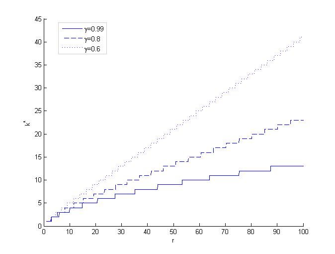
(a) Optimal $k^{*}$

(b) $C(k)$ with $\lambda_{1}=1$, $\lambda_{2}=9$, $\gamma=0.8$

Figure 1: Illustrations of $k^{*}$ and $C(k)$

The next theorem points out the relationship between the optimal $k$ and the discount factor $\gamma$ and two important limit cases. The proof follows immediately from (5).

Theorem 4

The optimal $k$ is decreasing with the discount factor $\gamma$. Furthermore, when $\gamma\rightarrow 1$, $k\sim\sqrt{2r}-1$ and when $\gamma\rightarrow 0$, $k\sim r$.

Theorem 4 is quite instrumental. It directly links the discount factor to the optimal frequency of serving each queue. In particular, when discount factor is small, then we are more focused on the current state, and we will choose the longer queue to serve at each moment. Under the state-independent assumption, this means that if the ratio between the arrival rates is $r$, then the ratio of the frequency of serving the two queues should be about $r$ (i.e., serve the slow-arrival queue only when it accumulates the same amount of customers as the long queue). On the contrary, when the discount factor goes to $1$, we have to be careful about the accumulation effect, that is, the accumulated waiting time for $k$ period for one queue is roughly of order $k^{2}$, and we want to serve the slow-arrival queue if $k^{2}$ is of order $r$. Therefore, the ratio of the frequency between serving the two queues should be about $O\left(\sqrt{r}\right)$. This rule, although simple, may provide important guidance for practitioners when they decide how frequent to serve each queue.

5 Numerical experiments

In this section, we conduct numerical experiments to verify our findings. The results are shown in Table 1.

$\gamma$	$r$	$k^{*}$	$C(1)$	$C(r)$	$C(k^{*})$	OPT	Gap(1)	Gap($r$)	Gap($k^{*}$)
0.6	1	1	5.00	5.00	5.00	4.62	8.29%	8.29%	8.29%
0.6	3	2	10.63	10.71	10.51	9.93	6.98%	7.81%	5.82%
0.6	5	3	16.25	15.76	15.51	14.91	8.96%	5.68%	3.97%
0.6	9	4	27.50	25.15	24.95	24.51	12.20%	2.63%	1.82%
0.8	1	1	10.00	10.00	10.00	8.85	13.04%	13.04%	13.04%
0.8	3	2	20.56	21.21	20.41	18.47	11.28%	14.80%	10.49%
0.8	5	2	31.11	31.12	29.51	27.27	14.06%	14.08%	8.18%
0.8	9	4	52.22	49.07	46.20	43.93	18.86%	11.68%	5.16%
0.99	1	1	200.00	200.00	200.00	167.86	19.14%	19.14%	19.14%
0.99	3	2	399.50	424.12	399.33	342.91	16.35%	23.43%	16.30%
0.99	5	2	599.00	630.82	565.33	500.30	19.49%	25.75%	12.86%
0.99	9	3	997.99	1032.23	871.87	718.22	25.37%	29.60%	9.75%

Table 1: Numerical results of our policies

In Table 1, the first and second column show the $\gamma$ and $r$ used. The third column is the optimal $k^{*}$ computed from (5). The fourth to sixth column are the expected costs when one uses a state-independent policy with serving $Q_{1}$ once followed by serving $Q_{2}$ $1$, $r$ or $k^{*}$ time respectively. The reason we choose $k=1$ and $k=r$ to compare is they are the simplest choices thus might be chosen in practice. The next column OPT is the optimal expected cost in the MDP. Note that OPT provides a lower bound of the cost for all state-independent policies. The last three columns in Table 1 show the cost gap between the state-independent policies and $OPT$. For all the numbers, we use $(M,\lambda_{2})$ as our initial state, which conforms to Theorem 2.

In Table 1, we see that the policy $k^{*}$ indeed performs much better than other choices. In particular, we see that choosing $k=1$ and $k=r$ usually result in comparable gaps from $OPT$, while choosing $k^{*}$ results in about half of the gaps. Furthermore, the gap becomes smaller when $r$ becomes larger, since if one queue has much faster arrival than the other, in either state-independent or dependent policy, one has to serve that queue more frequently, and the discrepancies between these two policies are smaller. Also, the gap becomes larger when $\gamma$ becomes larger, potentially due to that if the performance is evaluated in a long run, the ability to adjust to the current state is more important.

References

- Chaudhry and Templeton [1983] M. Chaudhry, J. Templeton, A First Course in Bulk Queues, Wiley, New York, 1983.
- Cooper [1981] R. Cooper, Introduction to Queueing Theory, 2nd ed, Elsevier, North-Holland, New York, 1981.
- Gross et al. [2008] D. Gross, J. Shortle, J. Thompson, C. Harris, Fundamentals of Queueing Theory, Fourth Edition, Wiley, 2008.
- Baras et al. [1985a] J. Baras, A. Dorsey, A. Makowski, Two competing queues with linear costs and geometric service requirement: the -rule is often optimal, Advances in Applied Probability 17 (1) (1985a) 186–209.
- Baras et al. [1985b] J. Baras, D. Ma, A. Makowski, K competing queues with geometric service requirements and linear costs: the -rule is always optimal, System and Control Letters 6 (3) (1985b) 173–180.
- Buyukkoc et al. [1985] C. Buyukkoc, P. Varaiya, J. Walrand, The rule revisited, Advances in Applied Probability 17 (1985) 237–238.
- Shanthikumar and Yao [1992] G. Shanthikumar, D. Yao, Multiclass queueing systems: polymatroidal structure and optimal scheduling control, Operations Research 40 (1992) 293–299.
- Dunne and Potts [1964] M. Dunne, R. Potts, Algorithm for traffic control, Operations Research 12 (6) (1964) 870–881.
- Deb [1978] R. Deb, Optimal dispatching of a finite capacity shuttle, Management Science 24 (1978) 1362–1372.
- Deb and Schmidt [1987] R. Deb, C. Schmidt, Optimal average cost policies for the two-terminal shuttle, Management Science 3 (5) (1987) 662–669.
- Ignall and Kolesar [1974] E. Ignall, P. Kolesar, Optimal dispatching of an infinite-capacity shuttle: control at a single terminal, Operations Research 22 (5) (1974) 1008–1024.
- Weiss [1979] H. Weiss, The computation of optimal control limits for a queue with batch services, Management Science 25 (4) (1979) 320–328.
- Weiss [1981] H. Weiss, Further results on an infinite capacity shuttle with control at a single terminal, Operations Research 29 (1981) 1212–1217.
- Lee and Srinivasan [1990] H. Lee, M. Srinivasan, The shuttle dispatch problem with compound Poisson arrivals: control at two terminals, Queueing Systems 6 (2) (1990) 207–221.