Horizontal or vertical magnetic fields on the quiet Sun:

Different analyses of identical Hinode SOT/SP data of quiet-sun magnetic fields have in the past led to contradictory answers to the question of whether the angular distribution of field vectors is preferentially horizontal or vertical. These answers have been obtained by combining the measured circular and linear polarizations in different ways to derive the field inclinations. A problem with these combinations is that the circular and linear polarizations scale with field strength in profoundly different ways. Here, we avoid these problems by using an entirely different approach that is based exclusively on the fundamental symmetry properties of the transverse Zeeman effect for observations away from the disk center without any dependence on the circular polarization. Systematic errors are suppressed by the application of a doubly differential technique with the 5247-5250 Å line pair for observations with the ZIMPOL-2 imaging polarimeter on the French THEMIS telescope on Tenerife. For the weakest, intranetwork-type magnetic fields, the angular distribution changes sign with the center-to-limb distance, being preferentially horizontal limbwards of $\mu$ (cosine of the heliocentric angle) $=0.2$, while favoring the vertical direction inside this disk position. Since decreasing $\mu$ corresponds to increasing height of line formation, this finding implies that the intranetwork fields are more peaked around the vertical direction in the low to middle photosphere, while they are more horizontal in the upper photosphere. The angular distribution is however also found to become more vertical with increasing flux density. Thus, all facular points that we have observed have a strong preference for the vertical direction for all disk positions, including those all the way to the extreme limb. In terms of spatial averages weighted by the intrinsic magnetic energy density, these results are independent of telescope resolution.

1 Introduction

Although the relation between the Zeeman-effect polarization and the magnetic field vector (strength and orientation) has been known for a century, most explorations of solar magnetic fields have been based on the longitudinal Zeeman effect alone, which gives us the line-of-sight component of the field. There have been relatively few attempts to determine the full field vector (starting with Stepanov & Severny 1962) by using the transverse Zeeman effect as well, but there are very good reasons for this. Firstly the measurement noise for weak to moderately strong fields is larger by typically a factor of 25 in the transverse field component as compared with the longitudinal field component, assuming that the polarization noise is the same for the circular and linear polarization measurements. In addition to this magnetic insensitivity, the relation between polarization and field strength is highly nonlinear (approximately quadratic) in the transverse Zeeman-effect case, in contrast to the nearly linear field-strength dependence on the circular polarization. It is this linear response that allows direct mapping of the line-of-sight component of the field. What usually goes under the name magnetogram is simply a map of the circular polarization recorded in the wing of a Zeeman-sensitive spectral line.

The nonlinear response of the linear polarization to the magnetic field creates a serious problem for the interpretation of the measurements. It is well known from past work with the longitudinal Zeeman effect that the magnetic structuring continues on scales far smaller than current resolution limits of solar telescopes (cf. Stenflo 2012). While the optical average over the spatial resolution element leads to a circular polarization that (because of its linear response) can be interpreted as a magnetic flux, the meaning of the corresponding optical average for the linear polarization depends on the poorly known properties of the subresolution magnetic structuring. It is therefore not so surprising that previous attempts to combine circular and linear polarization measurements to determine the vector magnetic field have led to highly divergent results.

Although the circular polarization alone only gives us one component of the field vector, it is possible to draw conclusions about the angular distribution of the field directions by examining how the appearance of the field pattern changes in line-of-sight magnetograms as we go from disk center to the limb and by comparing the appearance of magnetograms made in spectral lines formed at different heights. By comparing magnetograms in photospheric and in chromospheric lines, Giovanelli (1980) and Jones & Giovanelli (1983) thus concluded that the largely vertical magnetic field in facular regions rapidly diverges with height to develop a significant horizontal component with the formation of magnetic canopies having base heights of about 600-800 km, which are not far above the temperature minimum.

Since the application four decades ago of the 5250/5247 line-ratio method for the circular polarization (Stenflo 1973), we know that most of the flux that we see on the quiet Sun in full-disk magnetograms comes from strong (kG-type) fields. The main size range for these flux elements is estimated to be 10-100 km (Stenflo 2011), which is generally below the resolution of current telescopes, but there have been direct observations of resolved flux tubes since the upper tail of the size distribution falls in the domain that can be resolved. This was first accomplished by Keller (1992) by introducing the technique of speckle polarimetry and more recently by Lagg et al. (2010) with the IMaX magnetograph on the balloon-borne SUNRISE telescope. Pressure balance with the surroundings demands that the magnetic field lines of these flux elements must rapidly diverge with height because of the exponential decrease of the ambient gas pressure and therefore develop canopies in the upper layers. At the same time, the buoyancy, which also has its origin in the exponential height decrease of density and pressure, forces the magnetic configuration to stand upright. We therefore expect the flux from the intermittent flux elements (most often referred to as flux tubes) to be preferentially vertical in the lower photospheric layers and that the angular distribution will widen with height with an increasing proportion of highly inclined fields.

Although the kG fields are responsible for a major fraction of the net magnetic flux that we see in magnetograms with moderately high spatial resolution, they occupy only a low fraction of the photospheric volume of the quiet Sun. Through applications of the Hanle effect, we have long known (Stenflo 1982) that the remaining fraction is far from empty. On the contrary, it is seething with an “ocean” of flux that can be referred to as hidden, since it is invisible in medium-resolution magnetograms because of cancellation of the contributions from the opposite magnetic polarities within the telescope resolution element. However, it starts to emerge in magnetograms with high resolution, as in the Hinode data (Bellot Rubio & Orozco Suárez 2012). Since much of this field component is likely to be composed of elements that are expected to be much smaller than the atmospheric scale height (with sizes probably less than a few km, cf. Stenflo 2012), it has been natural to assume that their angular distribution is nearly isotropic.

The kG flux tubes and the microturbulent field represent two complementary idealizations in the description of the underlying reality. For theoretical reasons, we expect the weakest and strongest fields to be connected by a continuous field distribution with a continuous scale spectrum from the nearly global scales to the magnetic diffusion limit. In this continuum, we expect the weaker fields to be more tilted, since they are more easily buffeted by the turbulent or granular motions. Mixed-polarity fields of intermediate sizes will form a multitude of small loops, which will be characterized by largely horizontal fields at their tops. The question is then if all these various processes add up such that the total flux will on average be more vertical or more horizontal. In any case, we expect the relative proportion of horizontal fields to grow as we move up in height (cf. Steiner 2010).

In recent years there has been increasing use of the combination of the transverse and longitudinal Zeeman effects to derive both the strength and orientation of the magnetic field vector with the availability of imaging polarimeters that can record the full Stokes vector. Computer algorithms for this conversion (often referred to as Stokes inversion) have been developed and applied not only to active solar regions, where the S/N ratio of the data is good, but also to quiet regions, where the linear polarization signal for the majority of pixels is overwhelmed by noise.

Recordings of quiet-sun magnetic fields with superb spatial resolution by the SOT/SP instrument on the Hinode satellite (Kosugi et al. 2007; Tsuneta et al. 2008; Suematsu et al. 2008) reveal that not only vertical but also intermittent patches of horizontal magnetic fluxes can be found everywhere on the quiet Sun. Initial analysis of these data using the combination of the Stokes $V$ circular polarization signals with those of the linear polarization provided by Stokes $Q$ and $U$ led to claims not only that the angular distribution is more horizontal than vertical at the photospheric level of formation of the 6301 and 6302 Å lines that were used for the disk-center observations, but also that there is even as much as five times more horizontal than vertical flux (Orozco Suárez et al. 2007; Lites et al. 2008). In contrast, subsequent analysis of the identical Hinode data set led to the conclusion that the angular distribution is quasi-isotropic (Asensio Ramos 2009) or preferentially vertical, although becoming nearly isotropic in the weak flux-density limit (Stenflo 2010).

In these various investigations, the field inclination angles have been derived from different types of combinations of the observed circular and linear polarizations. The circumstance in which the obtained results are so divergent indicates that there are pitfalls in doing this. In the present work, we use an approach that aims at avoiding these pitfalls. By refraining from any comparison between the linear and circular polarization amplitudes and by instead basing our analysis on the linear polarization alone, as observed far away from the center of the solar disk to break the geometrical symmetry for the transverse Zeeman effect, we are able to determine for each center-to-limb position, whether the angular distribution favors the horizontal or the vertical direction. This method is model independent in the sense that it only makes use of the fundamental symmetry properties of the Zeeman effect.

2 Stokes profile signatures of field orientation

2.1 Symmetry properties of the Zeeman effect

The dependence of the emergent Stokes $Q$, $U$, and $V$ parameters on field strength $B$ and orientation (inclination $\gamma$ relative to the line of sight and azimuth $\chi$ relative to the direction that defines positive $Q$) can be expressed in the following factorized form(Stenflo 1994) as

$$Q = q_{\lambda}\,g_{Q}\,,$$

$$U = u_{\lambda}\,g_{U}\,,$$ (1)

$$V = v_{\lambda}\,g_{V}\,,$$

where nearly all of the angular dependence is contained in the angular factors of

$$g_{Q} = \sin^{2}\!\gamma\,\cos 2\chi\,,$$

$$g_{U} = \sin^{2}\!\gamma\,\sin 2\chi\,,$$ (2)

$$g_{V} = \cos\gamma\,,$$

while $q_{\lambda}$, $u_{\lambda}$, and $v_{\lambda}$ represent profile functions that describe the shape of the respective Stokes profile. In the optically thin case (weak-line limit), the profile functions depend on field strength $B$ but not on field orientation, and $q_{\lambda}=u_{\lambda}$. In the general case when the spectral lines are optically thick, $q_{\lambda}$ and $u_{\lambda}$ can differ from each other, but they are statistically identical for an axially symmetric field distribution. Each value of $q_{\lambda}$, $u_{\lambda}$, and $v_{\lambda}$ also has a weak dependence on field orientation, besides field strength, in the optically thick regime. This directional dependence has its origin both in line saturation (radiative-transfer effects) and magneto-optical effects and may mildly modify the shape of the profile functions but not their sign pattern.

For absorption lines, the central $\pi$ component of the transverse Zeeman effect is linearly polarized with the electric vector perpendicular to the direction of the transverse field component, while the blue- and red-shifted $\sigma$ component lobes are linearly polarized along the transverse field. For emission lines, we have the orthogonal polarization orientations. The signs of $Q$ and $U$ depend on the direction that we choose to define positive Stokes $Q$, but regardless of this definition the $\pi$ and $\sigma$ components of $q_{\lambda}$ and $u_{\lambda}$ have opposite signs.

The relative sign pattern of the transverse Zeeman-effect profiles (e.g. whether the $\pi$ component is positive or negative) is determined by the angular functions $g_{Q}$ and $g_{U}$. The weak directional dependence of $q_{\lambda}$ and $u_{\lambda}$ does not significantly change this qualitative aspect, although it modifies the shape and amplitudes. The analysis approach of the present paper is exclusively based on this qualitative symmetry property. It therefore does not depend on any assumptions concerning the field strengths (weak or strong) or line strength (optically thick line-formation effects).

Although the present work does not make direct use of the $B$ dependence of $q_{\lambda}$ and $u_{\lambda}$, this dependence plays a role in the understanding of the meaning of the spatial averages of the observed $Q$ and $U$ parameters, since it governs the weighting functions in the ensemble averages. If the Zeeman splitting is much smaller than the line width, both $q_{\lambda}$ and $u_{\lambda}$ of the linear polarization are proportional to $B^{2}$ or the magnetic energy density, while $v_{\lambda}$ of the circular polarization is proportional to $B$ or the magnetic flux. For the photospheric lines with which we are normally dealing, this weak-field case represents an excellent approximation for $B\la 0.5$ kG. We expect this regime to cover most of the intranetwork magnetic fields, although our analysis does not depend on this assumption.

The concept of using the symmetry properties of Stokes $Q$ distributions was introduced and applied long ago in center-to-limb observations of Stokes $Q$ (Stenflo 1987) to constrain the angular distribution of the spatially unresolved vector magnetic fields together with the field-strength constraints imposed on these hidden fields by the Hanle effect. The implementation of this concept was limited at that time by being based on observations with 1-pixel detectors (photomultipliers). With the availability of high-precision imaging Stokes polarimeters it is therefore only now that we are in a position to exploit the technique more fully.

2.2 Angular scaling functions in the atmospheric reference frame

The angular distribution functions that govern the signs of the Stokes $Q$, $U$, and $V$ parameters must be specified in the atmospheric reference frame relative to the vertical direction in the atmosphere, while the observed Stokes parameters have been expressed relative to the line of sight. We therefore need to convert the angles $\gamma$ and $\chi$ of the Stokes reference frame to the angle $\theta_{B}$ of the field vector relative to the vertical direction and azimuth $\phi$ of the field vector around the vertical, using the direction that defines positive $Q$ as projected onto the horizontal plane as the zero point. This conversion depends on the viewing angle, defined by the heliocentric angle $\theta$, which defines the center-to-limb distance of the observations at the same time.

With the help of spherical trigonometry, the converted expressions for the angular scaling factors in Eq. (2.1) become

$$g_{Q} = -\sin^{2}\!\theta_{B}\,\sin^{2}\!\phi\,+\,(\sin\theta\,\cos\theta_{B}\,-\mu\sin\theta_{B}\,\cos\phi\,)^{2}\,,$$

$$g_{U} = 2\sin\theta_{B}\,\sin\phi\,\,\,(\sin\theta\,\cos\theta_{B}\,-\mu\sin\theta_{B}\,\cos\phi\,)\,,$$ (3)

$$g_{V} = \mu\cos\theta_{B}\,+\,\sin\theta\,\sin\theta_{B}\,\cos\phi\,,$$

where $\mu=\cos\theta$. The symmetry direction that defines positive Stokes $Q$ and the zero point of the azimuths is the radius vector from disk center to the point of observation.

Next, we follow Stenflo (1987) and characterize the distribution over all the field inclination angles $\theta_{B}$ by the function,

$$f_{a}\,\sim\mu_{B}^{a}\,,$$ (4)

which is defined by the single free parameter $a$. Here, $\mu_{B}=\cos\theta_{B}$. The azimuth distribution is assumed to be axially symmetric (independent of $\phi$). The normalization constant is fixed by the requirement that the integration over all directions should give unity.

We can now conveniently classify the nature of the various angular distributions in terms of parameter $a$: An isotropic distribution is described by $a=0$, while a flat “pancake” distribution consisting of fields that are confined to the horizontal plane is represented by $a=-1$. As $a$ increases, the distribution increasingly peaks around the vertical direction. In the limit of infinite $a$, all fields are exactly vertical.

Let us already stress here that the results of the present paper, which are based on the qualitative symmetry properties of the $g_{Q}$ distributions, do not depend on the particular parametrization described by Eq. (4), although the particular choice of the $\mu_{B}^{a}$ distribution is made for mathematical and conceptual convenience.

Figure 1: Distribution of the angular scaling factors $g_{Q,U,V}$ of Eq. (2.2), representing the geometric scalings of Stokes $Q$ (solid line), $U$ (dashed line), and $V$ (dotted line). The scalings were computed by Monte Carlo simulations for the choice of an angular distribution parameter $a=1.5$ and a viewing angle defined by $\mu=0.3$.

We have used Monte Carlo simulations to explore the properties of the $g_{Q,U,V}$ distributions that result for a given choice of $a$ (angular-distribution parameter) and viewing angle (defined by $\mu$). Thus, each of the values for $g_{Q,U,V}$ is based on a pair of independent Monte Carlo samplings: one for $\phi$ based on a flat distribution and one for $\theta_{B}$ based on the distribution of Eq. (4). We use 20 million of these samples for each ($a$, $\mu$) combination to obtain smooth distribution functions. Figure 1 shows an example for the choice of $a=1.5$ (representing a distribution that favors vertical fields) and $\mu=0.3$ (representing a typical $\mu$ value of our observational data set).

The fundamental symmetry property is clearly brought out by Fig. 1: While the $g_{U}$ and $g_{V}$ distributions are symmetric relative to positive and negative values, the $g_{Q}$ distribution is not, as it strongly favors positive values. Therefore, an average over the distributions of $Q$, $U$, or $V$ values would give zero for $U$ and $V$ (assuming that the statistical sample used is sufficiently large), while the average of $Q$ would be nonzero. This symmetry property is valid for all viewing angles with the singular exception of disk center ($\mu=1.0$), where the $Q$ average also becomes zero because of symmetry around the vertical direction.

Figure 2: Distribution of the angular scaling factor $g_{Q}$ for $a=1.5$ and a sequence of $\mu$ values, decreasing from the disk-center value 1.0 (the symmetric solid line) to the extreme limb value of 0.0 in steps of 0.2. As $\mu$ decreases, the curves in the right-hand part of the diagram become increasingly elevated.

The asymmetry of the $g_{Q}$ distribution increases monotonically from zero as we go from disk center to the limb, as illustrated in Fig. 2, for the same choice of angular distribution parameter as in Fig. 1 ($a=1.5$). For negative values of $a$, the asymmetry goes in the opposite direction in favor of negative values. The more $a$ deviates from zero, the more pronounced the asymmetry becomes.

As we average $g_{Q,U,V}$ in Eq. (2.2) over the angular distribution defined by Eq. (4), we get zero for $g_{U,V}$, while the average $\bar{g}_{Q}$ of $g_{Q}$ is

$$\bar{g}_{Q}\,=\,{a\over a+3}\,(1-\mu^{2})$$ (5)

(Stenflo 1987). Note that $1-\mu^{2}=(r/r_{\odot})^{2}$, where $r/r_{\odot}$ is the radius vector in units of the disk radius $r_{\odot}$. Eq. (5) directly shows how the sign of $\bar{g}_{Q}$ determines whether the distribution is more vertical or more horizontal.

2.3 Relation between the $g_{Q}$ and $Q$ distributions

While the observed Stokes $Q$ scales with both $q_{\lambda}$ and $g_{Q}$, the profile function $q_{\lambda}$ has a fixed relative sign pattern between its $\pi$ and $\sigma$ components, although its detailed shape and amplitude scale with the field strength (in the weak-field regime in proportion to $B^{2}$). This sign pattern is either of the form $-+-$ or $+-+$. These two forms are governed by the angular function $g_{Q}$.

In our analysis approach, we deal with ensemble averages of field distributions. These distributions are functions of both field strength $B$ and field orientation. If the $B$ distribution were stochastically independent of the angular distribution, then the sign of the average ${\bar{Q}}$ of the observed $Q$ distribution would be determined exclusively by the sign of $\bar{g}_{Q}$, and spatial averaging over $Q$ would unambiguously determine whether the fields are more horizontal or more vertical. However, the angular distribution is $B$ dependent as will be shown in the present analysis, in the sense that the distribution becomes more peaked around the vertical direction as the flux density increases, as found earlier from Hinode quiet-sun disk-center analysis (Stenflo 2010). We know that there is a wide range of field strengths that coexist on the quiet Sun from near-zero to kG fields. In terms of our $a$ parameter that characterizes the angular distributions, this implies that there is a coexistence of a range of $a$-values.

To understand the meaning of the observed ${\bar{Q}}$ averages, let us subdivide the field-strength distribution in field-strength bins and consider the total vector field distribution (of both field strength and orientation) as a linear superposition of angular distributions with a different value of $a$ for each field-strength bin. The average ${\bar{Q}}$ is then obtained by first forming the angular averages of $Q$ for each field-strength bin and then the weighted sum of these averages over all the field-strength bins with $q_{\lambda}$ as weights is computed. Since $q_{\lambda}\sim B^{2}$ is a good approximation for field strengths below about 0.5 kG, the weighting function is approximately proportional to the pixel-average of the magnetic energy density. However, our analysis does not depend on any assumption concerning the validity of this approximation.

The meaning of the sign of ${\bar{Q}}$ depends on whether we refer $Q$ to the $\pi$ or $\sigma$ component amplitude of the transverse Zeeman effect (see below). For the present discussion, let us assume that positive ${\bar{Q}}$ means that the field distribution is preferentially vertical under the assumption of a $B$-independent angular parameter $a$. In the generalized framework of a $B$-dependent $a$, a positive ${\bar{Q}}$ then means that the distribution when weighted (approximately in terms of the magnetic energy densities) is preferentially vertical, while it is preferentially horizontal when ${\bar{Q}}$ is negative.

Since this weighting favors the contributions from the higher flux densities like facular points and, as we will see below, these fluxes are always strongly peaked around the vertical direction for all disk positions (all $\mu$ values), the contribution of the weak fluxes may easily get overwhelmed and masked by the domination of concentrated fields. As the main focus of the present work is to explore the angular distribution properties of the weakest fluxes, since they represent the only viable candidates for horizontal fields, we have particularly selected recordings in the most quiet, non-facular solar regions, where all the fluxes covered by the spectrograph slit are extremely weak (with very few pixels having $Q/I$ amplitudes in excess of 0.2 % and $V/I$ in excess of 0.5 %). The measurement of these weak polarization signatures has become possible thanks to the ZIMPOL technology, with which the polarimetric precision is almost exclusively limited by photon statistics. The 1-$\sigma$ error in the determination of the $Q/I$ amplitude is on the order of 0.01 % for each spatial pixel and is reduced by an order of magnitude when averaging over all pixels along the slit. By isolating these weak fluxes, the observationally determined averages ${\bar{Q}}$ will avoid the dominance of the higher flux densities and more closely approximate the angular-distribution properties in the weak flux limit, which is representative of what we may call the intranetwork fields.

2.4 Influence of the telescope resolution

The averaging over the values of $Q$ that gives us ${\bar{Q}}$ for a given area of the solar disk can be done in two different ways: (1) Optical integration over the area, or (2) numerical integration over the different resolved spatial pixels in the selected area. In practice, there is always a combination of the two, since the quiet-sun magnetic fields are at best only partially resolved. As the integration over Stokes $Q$ represents a linear superposition of the contributions from each infinitesimally small solar surface element, the results of an optical and a numerical integration however are identical. This would not at all have been the case if we would have averaged over flux densities or field strengths instead, since the relation between Stokes $Q$ and field strength is very nonlinear. As the observed $Q$ is however proportional to the number of polarized photons, optical and numerical summation are equivalent.

The consequence of this equivalence is that the average ${\bar{Q}}$ over a given area of the Sun’s surface is independent of telescope resolution. The average would not be different if we would use the substantially higher spatial resolution of Hinode, or any hypothetical future telescope with far higher angular resolution.

Let us for clarity stress that the resolution independence that we talk about here exclusively refers to the ensemble averages. The magnetic structuring that is directly revealed by the observations is, of course, extremely dependent on telescope resolution. With each new generation of solar telescopes, the solar images reveal a new world of structures that was not visible before. In the Stokes images presented in the present paper and elsewhere, structures of varying amplitudes, signs, and sizes are seen everywhere, and their visibility depends on telescope resolution. This dependence does not in any way contradict our arguments concerning independence of telescope resolution for the ensemble averages. The only assumption that is involved here is that the statistical sample used when calculating these ensemble averages is sufficiently large and representative. This is not a principle limitation, since it can be improved through increase of the size of the data base.

Similar resolution independence has been encountered 40 years ago with the Stokes $V$ 5250/5247 line ratio technique (which revealed the intermittent kG nature of quiet-sun magnetic flux) and 30 years ago with the application of the Hanle depolarization technique (which revealed the existence of the hidden, turbulent magnetic field). Since the unique power of all these methods is their independence of telescope resolution, observational applications of them give priority to polarimetric precision combined with high spectral resolution, while high spatial resolution is secondary.

3 Observations and reduction technique

3.1 ZIMPOL-2 at THEMIS

The data set used here was recorded on Tenerife with the ZIMPOL-2 polarimeter of ETH Zurich that was installed at the French THEMIS telescope, which has a 90 cm aperture and is nearly polarization-free at the location in the optical train where the polarization is being analyzed. Two observing campaigns with ZIMPOL on THEMIS have been carried out so far: one in 2007 (July 30 - August 13, 2007) and the other in 2008 (May 29 - June 12, 2008). The main aim was to explore the spatial structuring of the Second Solar Spectrum with its Hanle effect in different prominent spectral lines, but some recordings of the Zeeman effect were also carried out, in particular for the 5247-5250 Å data set used here.

The ZIMPOL (Zurich Imaging Polarimeter) technology (Povel 1995, 2001; Gandorfer et al. 2004) solves the compatibility problem between fast (kHz) polarization modulation and the slow read-out of large-scale array detectors by creating fast hidden buffer storage areas in the CCD sensor. This allows the photocharges to be cycled between four image planes in synchrony with the fast modulation. Linear combinations of the four image planes give us the simultaneous images of the four Stokes parameters. The images of the fractional polarizations, $Q/I$, $U/I$, and $V/I$, are free from both gaintable and seeing noise, because the flat-field effects divide out when the fractional polarizations are formed (since the identical pixels are used for the four image planes), and because the modulation is substantially faster than the seeing fluctuations.

The ZIMPOL-2 version creates the four fast buffers by placing a mask on the CCD (in the manufacturing process), such that three pixel rows are covered for buffer storage for every group of four pixel rows, while one is exposed. To prevent loss of 75 % of the photons that would fall on the masked part of the CCD, an array of cylindrical microlenses is mounted on top of the pixel array. Each cylindrical lens has the width of four pixels and focuses all the light on the unmasked pixels, thereby eliminating the light loss.

To modulate all four Stokes parameters simultaneously at about 1 kHz, we use two phase-locked ferro-electric liquid crystal (FLC) modulators in combination with a fixed retarder, followed by a fixed linear polarizer. By optimizing the relative azimuth angles of the three components in front of the polarizer, the modulator can be made sufficiently achromatic to be able to simultaneously modulate the Stokes parameters with high efficiency in two widely separated wavelength windows. Since our campaign employed two ZIMPOL-2 CCD sensors to exploit the opportunity offered at THEMIS to simultaneously observe in different parts of the spectrum, we needed this semi-achromatic optimization. The optimized settings led to a Mueller matrix of the modulator package that is highly nondiagonal in different ways at the selected wavelengths, but this is of no concern, since the matrix is always fully determined by the polarization calibration procedure and then numerically diagonalized. The only criterion is to simultaneously optimize the modulation efficiency in the four Stokes parameters.

The field of view for the observations was approximately 70 arcsec (along the slit) in the spatial direction and about 5.1 Å in the wavelength direction. The array size was 770 pixels in the wavelength direction multiplied by $4\times 140=560$ pixels in the spatial direction. Since the grouping of the pixel rows by the mask and microlenses is done in the slit direction, the effective number of spatial resolution elements was 140. The size of this effective resolution element corresponded to 0.5 arcsec on the Sun, which means that the effective (seeing-free) spatial resolution was limited to 1 arcsec. Seeing compensation was done with an active-optics tip-tilt system. The pixel size in the wavelength direction was 6.6 mÅ. The slit width was about 1.0 arcsec in the solar image, which corresponds to about 40 mÅ in the spectral focus.

The spectrograph slit was always oriented perpendicular to the radius vector, i.e., parallel to the nearest solar limb. In all our reductions and figures, the orientation of the Stokes system has been defined such that the positive $Q$ direction is parallel to the slit. In the 2-D spectral images, positive polarization signatures are brighter, and negative ones are darker than the surroundings.

Since the polarimetric sensitivity of the ZIMPOL system is practically only limited by the Poisson statistics of the collected photoelectrons, the S/N ratio scales with the square root of the effective integration time. Since polarimetric precision had the overriding priority over spatial and temporal resolution for the present type of work, very long effective integration times were used, usually 20-30 min, which is typical of explorations of the Second Solar Spectrum and the Hanle effect. These long integrations are also much needed when dealing with the miniscule signatures of the transverse Zeeman effect on the quiet Sun.

3.2 5247-5250 data set

The optimum region in the visible spectrum in terms of both sensitivity to the Zeeman effect and highest degree of model independence in magnetic-field diagnostics is the 5247-5250 Å range that includes the line pair Fe i 5247.06 and 5250.22 Å. This line pair is unique in several respects: As the two lines belong to the same multiplet (no. 1 of neutral iron), have the same line strength, and have the same excitation potential, they are formed in the same way in the solar atmosphere, in contrast to most other line combinations like the Fe i 6301.5 and 6302.5 Å lines, which differ significantly in their thermodynamic properties and heights of formation. The 5250 Å line has a Landé factor of 3.0, unsurpassed by any other relevant line in the Sun’s spectrum. It is therefore one of the most Zeeman-sensitive lines in the Sun’s visible spectrum. The only significant difference between the two lines of the pair is their Landé factors: For the 5247.06 Å line the effective Landé factor is 2.0, which is still large enough to also make this line highly Zeeman sensitive but is significantly different from 3.0, which makes this line combination an ideal “magnetic line ratio” for differential, nearly model-independent diagnostics.

The discovery of the kG nature of quiet-Sun magnetic flux was made by determining the differential Zeeman saturation from the ratio of the circular polarizations in these two lines (Stenflo 1973). Their identical line-formation properties allows a clean separation of the magnetic-field effects from the thermodynamic effects, although the sizes of the responsible flux elements are far lower than the telescope resolution. This insight laid the foundation for the construction of semi-empirical flux tube models, which were largely based on multiline analysis of recordings with an FTS (Fourier Transform Spectrometer) polarimeter (cf. Solanki 1993).

Here, we will not use the 5247-5250 line pair in the traditional way by forming Stokes $V$ or Stokes $Q$ line ratios, but we instead determine differential effects between the two lines when computing the spatial averages of Stokes $Q$. To eliminate the possible infiltration of subtle but systematic polarization effects at the level below 0.01 %, e.g. weak polarized fringes, we determine not only the $Q$ amplitude difference between the $\pi$ and $\sigma$ components of the transverse Zeeman pattern but also the difference between the two lines of these quantities. It is the use of these doubly differential quantities that allows an extraordinary precision in the determination of the angular distributions.

The recordings of the 5247-5250 Å range with ZIMPOL-2 at THEMIS were carried out on June 9-10, 2008. On the first day, a sequence of quiet-sun recordings at $\mu$ positions 0.1, 0.2, 0.3, 0.4, and 0.5 from the heliographic N pole along the central meridian were performed to provide us with a center-to-limb sequence of the most quiet Sun. Inspection of the recordings showed that none of the slit positions contained contributions from any facular points. All of them represented what we would call intranetwork. On the second day, recordings in a number of limb regions with various types of facular points (from tiny to medium size) and small spots and additional recordings in other quiet regions were made. A total of 14 high-quality Stokes spectra of the 5247-5250 Å range were thus secured.

3.3 Evidence of vertical or horizontal fields through visual inspection

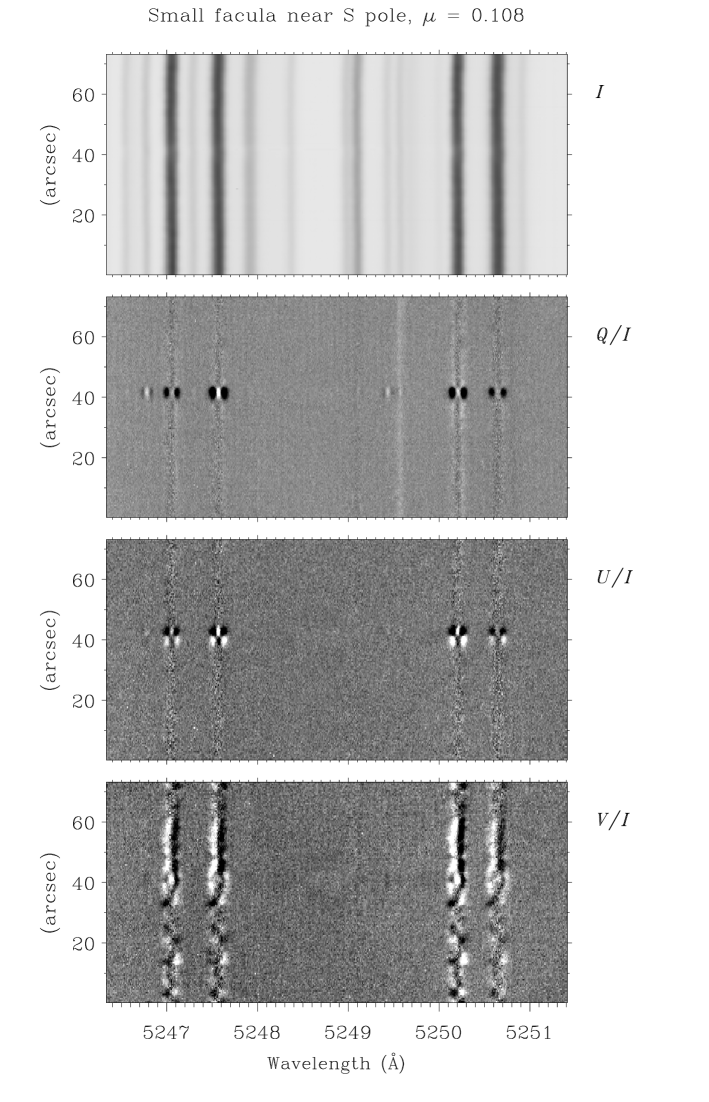
Figure 3: Stokes spectral images obtained with the slit crossing a small facula at $\mu=0.108$ near the heliographic S pole. The recording was made with ZIMPOL-2 at THEMIS on June 10, 2008. The transverse Zeeman-effect signatures in $Q/I$ show that the facular magnetic field is nearly vertical.

Figure 3 shows one example of such a recording (from June 10, 2008) across a small facula close to the solar limb at $\mu=0.108$ near the heliographic S pole. The facula stands out in the $Q/I$ and $U/I$ images with its spatially localized intense and symmetric polarization signatures from the transverse Zeeman effect, not only in the 5247.06 and 5250.22 Å lines, but also in the Cr i 5247.57 and Fe i 5250.65 Å lines with Landé factors of 2.5 and 1.5, respectively. In contrast, the antisymmetric $V/I$ profiles from the longitudinal Zeeman effect are not that localized but are conspicuous along most of the slit. Much of the reason for this difference in appearance between the transverse and longitudinal Zeeman effect has to do with their profoundly different relations between field strength and polarization. While this relation is nearly linear in the case of the circular polarization, it is highly nonlinear and approximately quadratic for the linear polarization. This leads to a relative magnification of the linear polarization in strong-field and relative suppression in weak-field regions.

When the sign of the polarization signatures of the transverse Zeeman effect with the central $\pi$ component of $Q/I$ is positive while the $\sigma$ components in the line wings are negative, this implies that the transverse component of the facular magnetic field is aligned with the radius vector, which for limb observations is evidence that the field is nearly vertical. If the transverse field had been perpendicular to the radius vector, the signs would have been reversed. For transverse fields that are $\pm 45^{\circ}$ to the radius vector, there would be no signal in $Q/I$, only in $U/I$ instead. The $U/I$ image shows a sign change across the facula. The signs are balanced, so that the spatially averaged $U/I$ almost vanishes. The presence of nonzero $U/I$ signatures shows that the facular field is not strictly vertical but has a significant angular spread around the vertical direction.

This sign behavior has been found for all faculae and spots for all center-to-limb positions that we have observed. Mere inspection of the Stokes spectra thus allows us to conclude that all these magnetic features have magnetic field distributions that peak around the vertical direction. Since the height of line formation increases as we move towards the limb, the field must retain the strong preference for a vertical orientation over the entire height range covered by our various $\mu$ values.

When we carefully inspect the slit region outside the small facula in Fig. 3 in the most Zeeman-sensitive line (5250.22 Å), we notice however a faint polarization signature that has a sign opposite to that of the facula almost all along the slit with positive $\sigma$ components and negative $\pi$ components. This is the signature for predominantly horizontal fields. It indicates that there is a profound dependence of the angular distribution on flux density: While the stronger isolated flux concentrations, like faculae, are found to be nearly vertical at all disk positions, the weakest background fields on the quiet Sun are preferentially horizontal near the solar limb.

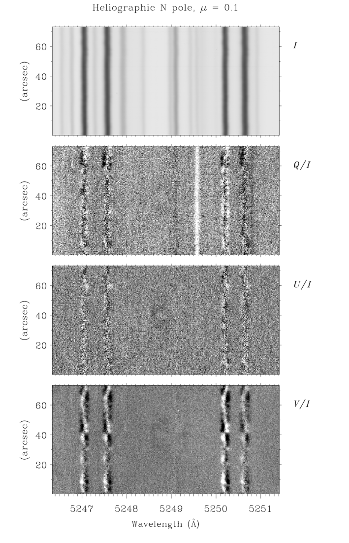
Figure 4: Stokes spectral images of a very quiet region (devoid of faculae) at $\mu=0.1$ near the heliographic N pole recorded with ZIMPOL-2 at THEMIS on June 9, 2008. Direct inspection reveals that the weak flux densities are preferentially horizontally oriented and that the great majority of the corresponding magnetic elements are unresolved.

We therefore need to turn our full attention to the weak background fields by selecting recordings of the most quiet regions, which are devoid of any facular points. Figure 4 shows a recording made at $\mu=0.1$ near the heliographic N pole. In contrast to Fig. 3 we can set the grey-scale cuts much lower to bring out the weakest signals, since there are no strong polarization features. Inspection of $Q/I$ for the 5250.22 Å line confirms the impression from Fig. 3 that the $\sigma$ components are predominantly positive and the $\pi$ component negative, as expected for preferentially horizontal fields.

Readers unfamiliar with the Second Solar Spectrum (the linearly polarized spectrum that is exclusively formed by coherent scattering processes) may be surprised by the bright emission-like line to the left of the 5250 Å line in the $Q/I$ panel. It was also seen in Fig. 3 but stands out in much higher contrast in Fig. 4 because of the lower setting of the grey-scale cuts. Like most rare earth lines in the Sun’s spectrum the Nd ii 5249.58 Å line (of singly ionized neodynium) exhibits strong scattering polarization (with the electric vector oriented parallel to the solar limb) (cf. Stenflo & Keller 1997) at the same time as it shows no trace of the Zeeman effect — an enigmatic behavior that is not yet understood. Near the limb, the continuous spectrum is also significantly polarized, mainly by coherent scattering in the distant wings of the Lyman series lines and by Thomson scattering (Stenflo 2005). The transverse Zeeman-effect signatures therefore sit on an elevated $Q/I$ continuum, which must be accounted for in the quantitative analysis.

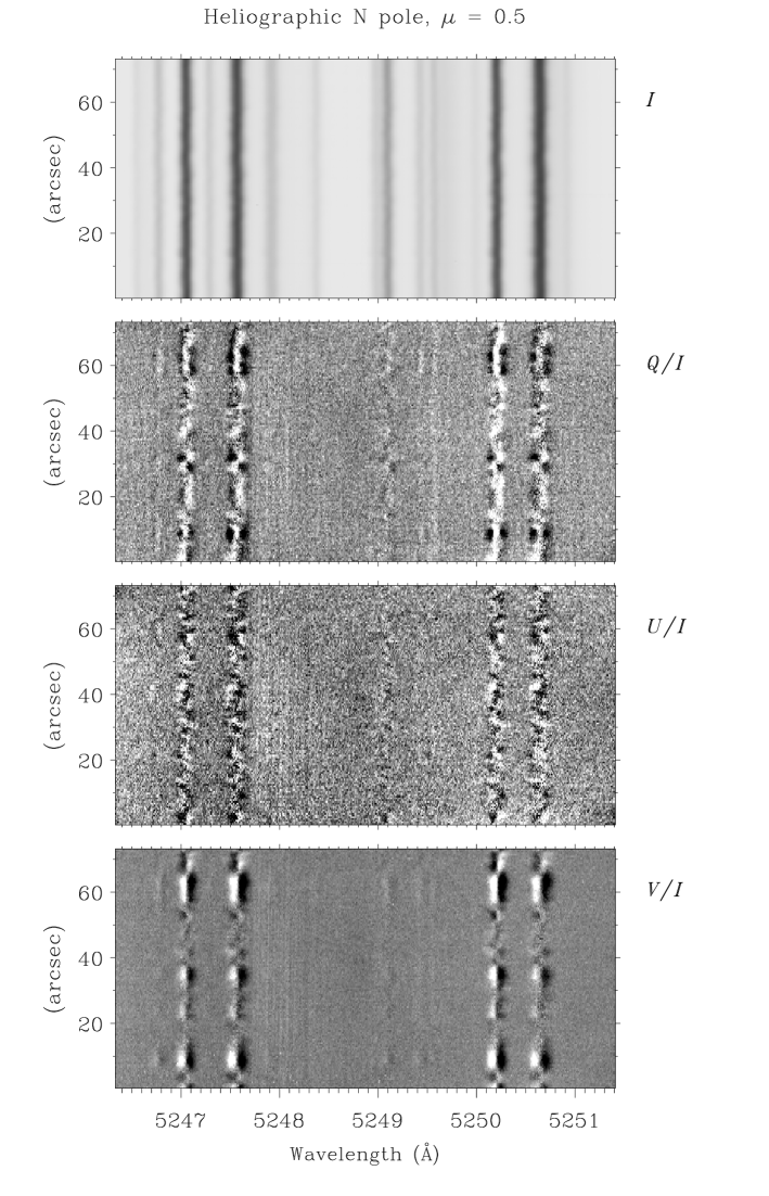
Figure 5: Same as for Fig. 4, except that the recording was made at a $\mu$ position of 0.5 near the heliographic N pole. Visual inspection reveals that for this larger $\mu$ value the weak flux densities have changed to be more vertically oriented.

As we move away from the limb, the angular distribution of the background fields becomes preferentially vertical, as shown by Fig. 5 for a very quiet region at $\mu=0.5$ near the heliographic N pole. Visual inspection of $Q/I$ of the 5250.22 Å line reveals that it is now the $\pi$ component that is predominantly positive, while the $\sigma$ components are more negative, which is the signature for predominantly vertical fields.

Direct inspection of Figs. 4 and 5 also allows us to conclude that the magnetic elements that collectively constitute the background field are much smaller than the telescope resolution. One telltale signature of the presence of multiple distinct magnetic elements within each spatial resolution element is the highly anomalous $U/I$ profile shapes in Fig. 5 with no resemblance of the well-known symmetry properties of the transverse Zeeman effect (approximate symmetry around line center). This can easily be understood in terms of the superposition of spatially unresolved magnetic elements, of which each has slightly different Doppler shifts because of their different positions within the solar granulation. It is well known from explorations of Stokes $V$ profiles (e.g. Sigwarth 2001) that the superposition of the contributions from unresolved magnetic elements with different relative Doppler shifts is the main cause of the observed anomalous Stokes $V$ profile shapes. This superposition does not have to be for different unresolved elements in the transversal plane. Anomalous $V$ profiles are also produced by correlated velocity and magnetic field gradients along the line of sight (Illing et al. 1975; Auer & Heasley 1978). Anomalous $Q$ and $U$ profiles are produced in the same way.

3.4 Extraction of Stokes parameters

After having demonstrated how far-reaching and model-independent conclusions can be made from pure visual inspection of the Stokes images, we now turn to the quantitative analysis of the images. Since we are dealing with very weak polarization signals, most of which have amplitudes in the range of 0.01 - 0.1 %, and the 1-$\sigma$ noise level is on the order of 0.01 % per spatial pixel, it is imperative to use a technique for the extraction of the Stokes profile amplitudes, which does not lead to skewed distributions for amplitudes comparable to or smaller than the noise, but which have a symmetric Gaussian error distribution. This ensures that the observational histogram (PDF) of Stokes profile amplitudes represents the intrinsic, noise-free histogram convolved with the Gaussian noise distribution.

This technique was developed and implemented in the analysis of quiet-sun Hinode SOT/SP spectra by Stenflo (2010), and it will be applied here as well. An average Stokes spectrum that has a high S/N ratio is used to construct templates. The blue and red $\sigma$ component lobes and the $\pi$ component lobe are cut out and amplitude normalized to become the templates for iterative least squares fitting of the Stokes spectrum for each spatial pixel. Before fitting, the spectrum is Doppler shifted and interpolated to the wavelength scale used for the template spectrum. The only free parameter in the least squares fit is the amplitude of the respective lobe, which is determined together with its standard error. This fitting procedure is extremely robust with immediate and entirely unique convergence. The error distribution is symmetric and Gaussian.

Figure 6: Slit average of the Stokes profiles recorded on June 10, 2008 in a facular region at $\mu=0.261$ near the heliographic N pole. Note the signature of a vertical field: positive $\pi$ components in $Q/I$, almost zero signal in the spatial average of $U/I$.

For the template spectrum we use the average along the spectrograph slit for a recording across faculae at $\mu=0.261$ near the heliographic N pole. This averaged spectrum is shown in Fig. 6. Since $U/I$ changes sign along the slit with a balanced sign distribution, the slit average of $U/I$ is nearly zero. In contrast $Q/I$ consistently has the same sign along the slit, since the fields remain nearly vertical.

Since the $Q/I$ and $U/I$ relative profile shapes from the transverse Zeeman effect are identical on average, the lobe templates that we cut out from the $Q/I$ profiles in Fig. 6 also serve as templates for least-squares fitting of the $U/I$ lobes. While the $V/I$ profiles have two lobes (the blue and red $\sigma$ components), the $Q/I$ and $U/I$ profile have three lobes to fit (because of the additional $\pi$ component).

Let us stress here that we make no assumption that the actual Stokes profiles resemble the template profiles in Fig. 6. As the amplitudes of each of the three profile lobes of $Q$ and $U$ (the $\pi$ and the two $\sigma$ components) are determined independently of each other, the profiles are allowed to have any anomalous balance between these components, like single-lobe profiles, same-sign lobes, etc. The determination is independent of the S/N ratio of the data, since each lobe amplitude is determined with an unbiased, symmetric, and well-defined Gaussian error distribution. This property represents the special strength of our extraction technique.

4 Angular distributions from the CLV of Stokes $Q$

4.1 Conclusions from direct visual inspection

Figure 7: Slit averages of the 2-D $Q/I$ spectra in Figs. 4 and 5. The zero point of the polarization scale, which should lie at the level of the dashed line, has been shifted to represent the continuum level, since the amplitudes of the Zeeman effect are measured relative to the continuum. The dotted vertical lines mark the line centers of the 5247.06 and 5250.22 Å lines. The reversal of the sign of the transverse Zeeman effect from $\mu=0.1$ to $\mu=0.5$ shows that the angular distribution changes from predominantly horizontal to vertical as we move away from the limb.

In Sect. 3.3, we concluded from visual inspection of Figs. 4 and 5 that the $Q/I$ profiles had opposite signs on average in the two figures and that therefore the weak background magnetic fields on the quiet Sun change from being predominantly horizontal near the extreme limb to become preferentially vertical when we move away from the limb. This implies a corresponding height variation in the angular distribution, a property that is brought out more clearly in Fig. 7, which shows the spectra of Figs. 4 and 5 after averaging along the spectrograph slit. Since the linear polarization of the transverse Zeeman effect sits on top of an elevated continuum that is polarized by processes (Rayleigh and Thomson scattering) that are irrelevant to our Zeeman-effect analysis, we have shifted the zero point of the $Q/I$ polarization scale so that it represents the continuum, relative to which the amplitudes of the line-profile lobes that are caused by the Zeeman effect are measured. The true zero point of the polarization scale is indicated by the dashed line in the two panels. Since the scattering polarization increases steeply towards the limb, the shift is much larger for $\mu=0.1$ than for $\mu=0.5$. Similarly, the polarization amplitude of the neodynium line at 5249.58 Å decreases steeply as we move away from the limb.

Figure 7 clearly shows that the $\pi$ component for $\mu=0.1$ points in the negative direction and the $\sigma$ components in the positive direction, which indicates a preference for horizontal fields. For $\mu=0.5$ the signs however are reversed and represent preferentially vertical fields.

Careful inspection of Fig. 7 indicates that the continuum level that serves as our reference level for the Zeeman effect is not entirely flat but there seem to be large-scale fluctuations on the order of 0.005 %, possibly beacuse of weak polarized fringes. To eliminate errors that are caused by this effect we will not describe the transverse Zeeman effect in terms of the amplitudes of the $\pi$ and $\sigma$ components alone, but instead in terms of the amplitude difference between the $\pi$ component and the average of the blue and red lobe $\sigma$ components. This difference is insensitive to the level of the continuum or zero point of the polarization scale. By using the average of the blue and red lobe $\sigma$ components, we effectively symmetrize the $Q/I$ profiles to avoid issues with the anomalous profiles that are caused by the superposition of subpixel structures with different Doppler shifts. The use of these differential techniques is crucial for all diagnostic work to isolate the phenomenon of interest from possible contamination from a multitude of undesired effects.

4.2 Histogram properties

Figure 8: Histograms of $Q/I$ (solid) and $U/I$ (dashed) for the 5250.22 Å line, which are sampled along the spectrograph slit for the two Stokes spectra illustrated in Figs. 4 and 5. The measured quantity is the difference between the $\pi$ component and the average of the two $\sigma$ components. The error bars for a single pixel are indicated (with asterisk representing $Q/I$, cross $U/I$). While the $U/I$ distributions are symmetric around zero, the $Q/I$ distributions are skewed in favor of horizontal fields in the upper panel and in favor of vertical fields in the bottom panel.

While Fig. 7 shows the slit average of the 2-D spectra in Figs. 4 and 5, Fig. 8 shows the histogram distributions of all the pixels along the slit of the same Stokes spectra, for $Q/I$ (solid curves) and $U/I$ (dashed curves) of the 5250.22 Å line. The quantity that is represented by the histograms is the amplitude difference between the $\pi$ component and the average of the two $\sigma$ components, which is insensitive to errors in the zero point of the polarization scale or the continuum level.

While the $U/I$ distributions are symmetric around the zero point for both $\mu$ positions as expected for symmetry reasons, the $Q/I$ distributions are strongly asymmetric, showing that the angular distributions differ significantly from the isotropic, symmetric case. For $\mu=0.1$, the asymmetry strongly favors negative values, implying preferentially horizontal fields, while it strongly favors the positive values for $\mu=0.5$, implying preference for vertical fields. Since the widths of the distributions are substantially larger than the 1-$\sigma$ error bars, the spread of the values is of solar origin for the most part (as seen with the resolving power of the telescope).

One may think of the distributions in Fig. 8 as one part of a sum that is symmetric and the rest that is non-symmetric. When forming the slit averages to obtain Fig. 7, the contribution from the symmetric part vanishes, and all the contribution comes from the lop-sided non-symmetric part.

While the symmetry properties of the histograms are those of the angular scaling functions $g_{Q}$ and $g_{U}$ that were discussed in Sect. 2.2, the histogram shapes cannot be directly compared with these functions, since the observed $Q/I$ and $U/I$ are proportional not only to the angular functions but also approximately to $B^{2}$, the square of the field strength. In addition, the shape of the angular distribution is a strong function of field strength. The importance of the angular scaling functions of Sect. 2.2 is to show how the preference for a horizontal or a vertical field distribution arises from the sign of the $g_{Q}$ asymmetry, independent of any assumption for the $B$ distribution.

4.3 Height transition from vertical to horizontal preference

So far, we have focused our attention only on the two recordings represented by Figs. 4 and 5, to illustrate very explicitly the physical basis for our conclusions about the angular distributions. In our next figures, we represent diagrams of the types in Figs. 7 and 8 by a single data point per $\mu$ value and spectral line.

From our 5247-5250 data set of 14 $\mu$ positions, seven represent regions devoid of any faculae, which we select here as representative of the quiet-sun background (or intranetwork) fields. We have verified that there is no subtle influence from any facular point by comparing the results for two separate slit averages: (1) taking the average of all the pixels, or (2) only averaging the pixels for which $V/I<0.5$ %. For all the seven selected regions, the two slit averages result in the same $Q/I$ profile amplitudes, in clear contrast to the remaining seven regions with faculae. For the facular regions the full slit averages always show the fields to be strongly vertically oriented at all $\mu$. There is only evidence of horizontal fields near the limb for the weak background fields.

The seven background-field regions consist of the five recordings along the central meridian from the heliographic N pole from $\mu=0.1$ to 0.5 in steps of 0.1 plus two recordings near the heliographic E limb at $\mu=0.08$ and 0.132.

So far, we have focused the discussion on the behavior of the 5250.22 Å line, since it is the most Zeeman-sensitive of the lines and therefore has the highest S/N ratio. We have not yet made use of the opportunity of having a companion line (5247.06 Å) within the field of view with the same line-formation properties that only differ in Landé factor. For the transverse Zeeman effect, the expected linear polarization amplitudes of the two lines should (in the weak-field limit, for $B\la 500$ G) be approximately proportional to the square of the respective Landé factors for the 5250/5247 ratio, thus proportional to $9/4=2.25$. We should expect to find the same results from the two lines but with a smaller amplitude in the 5247 Å line.

Figure 9: Amplitude of the $Q/I$ $\pi$ component (upper panel) and the average of the blue and red lobe $\sigma$ components (bottom panel) as a function of $\mu$ for the 7 solar regions with only weak background intranetwork-type fields. Filled circles: 5250.22 Å line. Open circles: 5247.06 Å line. The dashed line represents the position of the polarization zero level before being shifted to the continuum level.

In Fig. 9, we have plotted the $\pi$ component amplitudes that have been extracted from the seven recordings (upper panel) and the average of the blue and red $\sigma$ components (bottom panel) as filled circles for the 5250 Å line, as open circles for the 5247 Å line as a function of $\mu$. For reference, the dashed line represents the true position of the polarization zero level owing to the continuum polarization before shifting the zero to the continuum level used as the reference level for the Zeeman effect analysis.

In Fig. 9, we have not plotted the $\pi-\sigma$ difference like in Fig. 8 but plotted the absolute values of the separate components. These values are susceptible to errors in the polarization zero level used, and the errors may, in addition, be different for the two lines, if they are caused by weakly polarized fringes. This is the reason why the positions of the points look inconsistent and demonstrates why it is so important to use differential measures, such as the $\pi-\sigma$ amplitude difference used in Fig. 8. This differential measure is obtained by subtracting the values in the lower panel of Fig. 9 from the corresponding values in the upper panel. It is not meaningful to go into a detailed interpretation of Fig. 9 before having formed these differential measures. Instead, the figure illustrates the possible pitfalls of an analysis that is not differential.

Figure 10: Difference between the $\pi$ and $\sigma$ components for the 5250 Å line minus the corresponding difference for the 5247 Å line, plotted as a function of $\mu$ for our seven intranetwork regions. The negative values show that the angular distribution is preferentially horizontal limbwards of $\mu=0.22$ (the zero crossing of the straight-line fit), while it is preferentially vertical on the diskward side.

These $\pi-\sigma$ differentials can be formed separately for the 5250 and 5247 Å lines from the difference between the two panels in Fig. 9. These differentials should show the same behavior for the two lines, except with much smaller amplitude for the 5247 Å line. In Fig. 10, we go a step further to create a double differential by forming the difference between the $\pi-\sigma$ differential for the 5250 Å line and the corresponding differential for the 5247 Å line. By doing so, we doubly suppress systematic errors that can arise from fringes and varying polarization background levels.

Besides random measurement noise the remaining scatter of the points around the straight-line fit in Fig. 10 is mainly related to the finiteness of our modest statistical sample of solar resolution elements (140 effective spatial pixels for each of the 7 Stokes images). In this sense, the scatter of the points is partly solar in origin, and it is therefore not so meaningful to assign error bars to them. Note that the standard deviation of the scatter of the points around the straight-line fit is only $5\times 10^{-5}$, much of which is of solar origin.

In terms of this doubly differential measure, positive values correspond to angular distributions that are more peaked around the vertical direction (in comparison with the isotropic distribution), while negative values represent angular distributions that favor the horizontal plane. The zero crossing of the straight-line fit in Fig. 10 occurs at $\mu=0.22$. Limbwards of this center-to-limb position, the intranetwork fields are preferentially horizontal, while diskwards they are preferentially vertical. This confirms the qualitative conclusions in a more quantitative way that we could draw from plain inspection of the slit-averaged Stokes spectra.

5 Interpretation and conclusions

5.1 Height and flux-density dependence

The height of line formation increases with decreasing $\mu$, when we move closer to the limb. Our finding that the $\pi-\sigma$ amplitude changes sign around $\mu=0.22$ for the weak background fields implies that the angular distribution of the field vectors is more pancake-like (horizontal) in the upper photosphere near the temperature minimum and above, while it is more vertical in the middle photosphere and below. For disk-center observations of spectral lines like the 5247-5250 or the 6301-6302 line pairs, the distribution is always more vertical (than the isotropic case), which confirms our previous conclusions from the analysis of Hinode observations (Stenflo 2010).

There is a close relation between angular distribution and flux density. The stronger flux densities remain peaked around the vertical direction for the whole height range covered by our various $\mu$ values. This is consistent with our previous Hinode results (Stenflo 2010) that the degree of concentration around the vertical direction increases steeply with flux density, while the distribution tends to become nearly isotropic in the limit of low flux densities. In the present work, we find that as we move up in the atmosphere, the distribution does not approach the isotropic case in the limit of low flux densities but changes from being more vertical to becoming more horizontal above a certain level.

Here, we have made the distinction between solar regions containing faculae and regions with background fields devoid of facular points, but we could also have used the terminology network and intranetwork. Thus network flux remains preferentially vertical throughout the considered height range. In contrast, intranetwork fields are preferentailly vertical in the lower and middle photosphere but become preferentially horizontal in the higher layers.

While there is a correspondence between $\mu$ value and geometrical height, a quantitative translation of $\mu$ into a height scale would require radiative-transfer modelling, which is outside the scope of the present work.

5.2 Roles of buoyancy and stratification

The outer envelope of the Sun is highly stratified with a steep outwards decrease in the gas pressure. This has important consequences for the height dependence on the magnetic field, which is governed by three main factors: buoyancy, containment of the magnetic pressure, and topology (in particular the scales of polarity mixing).

As the magnetic flux concentrations are partially evacuated to satisfy pressure equilibrium with the surroundings, they become subject to strong buoyancy forces. Field lines that are anchored (by the frozen-in condition) in the dense deeper layers will be forced by buoyancy towards the upright orientation. Buoyancy tries to generate angular distributions that are peaked around the vertical direction.

The equilibrium between magnetic pressure and ambient gas pressure shifts rapidly in favor of the magnetic pressure as we move up in height. This means that any magnetic-field concentration will expand and the field lines flare out. For this reason, the angular distribution will contain a larger proportion of highly inclined fields in the higher layers.

Numerical simulations of magneto-convection do indeed show that the magnetic field becomes more horizontal in the upper photospheric layers (Abbett 2007; Schüssler & Vögler 2008; Steiner et al. 2008). The maximum height of magnetic flux loops scales with the separation of their footpoints at the bottom of the photosphere. Near the top of the loops, the flux is largely horizontal. The smaller the polarity mixing scale of the flux footpoints, the lower is the loop height, which means a lower transition height in the atmosphere from a vertical to a horizontal field distribution (cf. Steiner 2010).

We thus have a competition between buoyancy, which favors vertical fields, and the other two effects (flux expansion and polarity mixing), which lead to an increasing proportion of inclined fields as we move up in height. We expect the height at which buoyancy loses to the other effects to depend on field strength, since the magnitude of the buoyancy force scales with field strength. Therefore, stronger fields are expected to retain their vertical preference at greater heights, as observed. In contrast, the weakest fluxes are not only less affected by buoyancy, but they are also more easily buffeted by the dynamic pressure of convective turbulence and thereby develop more small-scale polarity mixing. While the quiet-sun network fields tend to be fairly unipolar (on the supergranulation scale), the intranetwork fields are thus characterized by mixed polarities on small scales.

Observations with 3 arcsec spatial resolution of the temporal variations in the line-of-sight component of this intranetwork field reveal that it is highly dynamic and that its fluctuations get much more pronounced near the solar limb (Harvey et al. 2007). This is evidence of a dynamic horizontal field component in the upper photosphere (where the spectrum observed near the limb originates). A related result has been obtained from Hinode observations by Lites (2011), who finds an increased line-of-sight flux density for the intranetwork fields as one goes from disk center towards the solar limb. Part of this effect is owing to the circumstance that the intranetwork field has a wide angular distribution, and part of it is a height variation. However, these observations do not tell in which sense the angular distribution deviates from the isotropic case (for instance in favor of horizontal fields), and whether this deviation changes sign with height. This is the issue that is being addressed by our present analysis.

Hanle-effect observations have shown that the photosphere is seething with an ocean of mixed-polarity fields on scales on the order of a few km or less. The atmospheric stratification becomes increasingly irrelevant as we go to smaller and smaller tangled magnetic structures in the size domain below the scale height. Because of scale separation, the angular distribution may be expected to approach the isotropic case in the small scale limit.

5.3 Model independence of the conclusions

Our method to determine whether the angular distribution of field vectors is more horizontal or more vertical as compared to the isotropic distribution is model independent in the sense that it only depends on the fundamental symmetry property of the transverse Zeeman effect: If $\pi-\sigma$ for the spatially averaged $Q/I$ is positive, then the field distribution is more vertical, while it is more horizontal if it is negative. The magnitudes of the polarization values never enter in this decision, only the sign. By forming double differentials, like the difference of the $\pi-\sigma$ values between the 5250 and the 5247 Å lines, we suppress possible systematic errors.

This approach does not depend on the particular choice of parametrization of the magnetic-field distribution functions given by Eq. (4), since the qualitative symmetry properties describing the relation between the sign of the average $Q/I$ and the horizontal-vertical preference would be the same with any choice.

Note that we do not try in the present paper to convert polarization values into field strength or $\mu$ values into geometrical height but limit our determination to the variation in the sign of the vertical-horizontal preference with center-to-limb distance. A conversion to geometrical height and to field strength values at these heights would require radiative-transfer modelling and make the results model dependent. By letting this be outside the scope of the present paper, we keep the results that are presented here model independent in the sense described.

5.4 Independence of angular resolution

While improvements of angular resolution are necessary to advance our knowledge about the morphology and evolution of solar magnetic fields, several of the main fundamental insights into the nature of quiet-sun magnetic fields have not depended on the resolving power of the telescope used. Examples are as follows: The extreme intermittency with much of the total quiet-sun magnetic flux being carried by collapsed, kG-type fields was discovered with an angular resolution of several arcsec thanks to the near model-independence that is a unique property of the 5250-5247 line ratio (Stenflo 1973). The discovery that the photosphere is seething with vast amounts of hidden magnetic flux with strengths in the range of 10-100 G was made by interpreting observations of the Hanle effect depolarization with a resolution on the order of one arcmin (Stenflo 1982). Similarly, the use of distribution functions for the transverse Zeeman effect to derive model-independent constraints on the angular distribution functions of quiet-sun magnetic fields, which has been the topic of the present paper, does not depend on the resolving power of the telescope, as clarified in Sect. 2.4. Although this method was known and applied more than a quarter of a century ago (Stenflo 1987), it is only now that we are in a position to more fully exploit it. The reason is not because of the improved angular resolution but because of the advances in high-precision imaging Stokes polarimetry, in particular through the availability of the ZIMPOL technology. In contrast, the 1987 investigation was based on observations with single-pixel detectors (photomultipliers).