A formula for damping interarea oscillations
with generator redispatch

Abstract

We derive a new formula for the sensitivity of electromechanical oscillation damping with respect to generator redispatch. The formula could lead to some combination of observations, computations and heuristics to more effectively damp interarea oscillations.

1 Introduction

Large-scale power systems have multiple low frequency and lightly damped electromechanical modes of oscillation. If the damping of these modes becomes too small or positive, then the resulting oscillations can cause equipment damage, malfunction or blackouts. The oscillations can appear for large or unusual power transfers, and may become more frequent as power systems experience greater variability of loading conditions. Practical limits for power system security often require sufficient damping of oscillatory modes [5, 27] and power transfers on tie lines are sometimes limited by oscillations [5, 16, 17, 4].

There are several approaches to suppressing low-frequency oscillations, including limiting power transfers, installing closed loop controls, and taking control actions such as redispatching generation. In this paper we do analysis to underpin the suppression of oscillations via redispatch of generation. Changes in generator dispatch change the oscillation damping by exploiting the nonlinearity of the power system: changing the dispatch changes the operating equilibrium and hence the linearization of the power system about that equilibrium that determines the oscillatory modes and their damping. The use of generator dispatch to damp oscillations has been demonstrated and there are several previous approaches:

1. There are heuristics in terms of the mode shapes for the redispatch for some simpler grid structures [11, 12].

2. There are exact computations of the sensitivity of the damping from a dynamic power grid model [8, 9, 22, 32]. The formulas from these computations require Hessians and left eigenvectors of the mode shapes, or derivatives of eigenvectors.

3. The effective generator redispatches can be determined by repetitive computation of eigenvalues of a dynamic power grid model to give numerical sensitivities [4, 14, 15, 7].

The requirement in approaches 2 and 3 of a large scale power system dynamic model poses some difficulties. It is challenging to obtain validated models of generator dynamics over a wide area and particularly difficult to determine dynamic load models. Moreover, in approach 2, it does not seem feasible to estimate the left eigenvectors of the mode shapes or derivatives of eigenvectors from measurements.

The new formula for modal sensitivity we derive largely depends on power system quantities that can, at least in principle, be observed from measurements. In particular, the formula shows that the first order effect of a generator redispatch largely depends on the mode shape and the power flow. (The assumed equivalent generator dynamics only appear as a factor common to all redispatches.) The mode shape (right eigenvector of the oscillatory mode of interest) is to some considerable extent obtainable from power system measurements [13, 29, 3, 10]. As a general goal, we would like to move towards approaches that take more advantage of synchrophasor measurements, and are less dependent on detailed wide area power system dynamic models that are hard to obtain. While we have not yet proved that the formula can be the basis for doing this, the formula does open up this promising possibility.

Another possible approach would be to use the new formula to gain insights into oscillation damping by generator redispatch that can be expressed and applied as heuristics. In fact our analytic work is inspired by the heuristics by Fisher and Erlich in [11, 12], and a general goal is to confirm, refine and extend their heuristics by supplying an analytic basis for the heuristics.

A key barrier to better understanding and computing or deriving heuristics for generator redispatch to damp oscillations has been the difficulty of the analysis. In this paper we are able to combine several new and old methods of analysis to derive a new formula for the sensitivity of the oscillation damping and frequency with respect to generator redispatch. Most of the paper is devoted to deriving the new formula, but we also give some special cases and simple examples to begin the process of understanding the formula and how it might be applied. The paper results will also appear in Spanish as part of PhD thesis [21].

2 Notation

We use the following notation and definitions. All quantities are in per unit unless otherwise stated.

$n$	number of buses
$m$	number of generator buses;
	buses 1,2,  … ,$m$ are the generator buses
$\ell$	number of transmission lines
$\delta_{i}$	voltage angle of bus $i$
$\delta$	vector of voltage angles $(\delta_{1},\delta_{2},...,\delta_{n})^{T}$
$V_{i}$	voltage magnitude at bus $i$
$V$	vector of voltage magnitudes $(V_{m+1},V_{m+2},...,V_{n})^{T}$
	at load buses
$z$	state vector $(\delta,V)^{T}$
$V_{i}^{\rm ln}$	${\rm ln}V_{i}$; logarithm of voltage magnitude at bus $i$
$P_{i}$	net real power injection at bus $i$
$Q_{i}$	net reactive power injection at bus $i$
$\omega_{0}$	nominal frequency in rad/s
$h_{i}$	inertia at bus $i$ in seconds
$m_{i}$	$2h_{i}/\omega_{0}$
$M$	diagonal matrix ${\rm diag}\{m_{1},m_{2},...,m_{{2n-m}}\}$
$d_{i}$	damping coefficient at bus $i$ in seconds
$D$	diagonal matrix ${\rm diag}\{d_{1},d_{2},...,d_{{2n-m}}\}$
$b_{ij}$	imaginary part of $ij$ element of bus admittance
	matrix (for $i\neq j$, $b_{ij}$ is the absolute value of the
	susceptance of the line joining bus $i$ and bus $j$;
	$b_{ii}$ is the sum of the susceptances incident on bus $i$.)
$b_{k}$	absolute value of the susceptance of line $k$
$p_{k}$	real power flow in line $k$ defined in (62)
$q_{k}$	part of reactive power flows in line $k$ defined in (61)
$R$	scalar potential energy function defined in (3)
$L$	a weighted Laplacian matrix; Hessian of $R$
$L^{\dagger}$	Matrix pseudo-inverse of $L$
$Q$	$M\lambda^{2}+D\lambda+L$; a quadratic matrix function of $\lambda$
$x$	eigenvector of $Q$

The bus-line incidence matrix $A$ is defined by

$$A_{ik}=\left\{\begin{array}[]{rl}1&\text{if bus $i$ is the sending end of line $k$,}\\ -1&\text{if bus $i$ is the receiving end of line $k$,}\\ 0&\text{otherwise.}\end{array}\right.$$ (4)

The matrix of absolute values of the entries of $A$ is written as $|A|$. That is,

$$|A_{ik}|=\left\{\begin{array}[]{ll}1&\text{if bus $i$ is the sending or receiving end of line $k$,}\\ 0&\text{otherwise.}\end{array}\right.$$ (7)

The angle across line $k$ is defined as

$$\theta_{k}=\sum_{r=1}^{n}\!A_{rk}\delta_{r}=\left\{\begin{array}[]{ll}\delta_{i}-\delta_{j}&\text{if bus $i$ is sending end of line $k$},\\ \delta_{j}-\delta_{i}&\text{if bus $i$ is receiving end of line $k$},\\ \end{array}\right.$$ (10)

and we write $\theta=(\theta_{1},\theta_{2},....,\theta_{\ell})^{T}$ for the vector of angles across all the lines.

The new voltage coordinate for line $k$ that connects bus $i$ to bus $j$ is defined by

$$\nu_{k} =\sum_{r=1}^{n}|A_{rk}|\ln{V_{r}}=\ln{(V_{i}V_{j})},$$

and we write $\nu=(\nu_{1},\nu_{2},....,\nu_{\ell})^{T}$ for the vector of voltage coordinates for all the lines.

$z^{\prime}$	state vector $(\theta,\nu)^{T}$ (“dashed” coordinates)
$h$	$z^{\prime}=h(z)$; transforms undashed to dashed coordinates
$H$	Jacobian of coordinate change $h$
$x^{\prime}$	eigenvector of $Q$ in dashed coordinates $z^{\prime}$

3 Power System Model

We model the generators with simple swing dynamic equations and also consider the real and reactive power balance algebraic equations of the network. The transmission lines are lossless.

The real power balance equations for all buses are

$$m_{i}\ddot{\delta}_{i}+d_{i}\dot{\delta}_{i}+\sum_{j\sim i}b_{ij}V_{i}V_{j} \sin(\delta_{i}-\delta_{j})=P_{i},$$

$$i=1,2,\ldots,n.$$ (11)

The notation $j\sim i$ means that the summation is over all buses $j$ connected to bus $i$, excluding $i$.

The reactive power balance equations for all load buses are

$$-\sum_{j\sim i}b_{ij}V_{j}\cos(\delta_{i}-\delta_{j})= \,\frac{Q_{i}}{V_{i}}+b_{ii}V_{i},$$

$$i=m+1,\ldots,n.$$ (12)

Note that the reactive power balance equations (3) have been divided by the bus $i$ voltage magnitude $V_{i}$ [6].

The model (3) and (3) is differential-algebraic equations written in terms of state variables $z=(\delta,V)$ of the bus voltage angles $\delta$ and the voltage magnitudes of the load buses $V$. (The generator voltage magnitudes $V_{1},V_{2},...,V_{m}$ are assumed to be constant.) The coupling of the machine angle dynamics of (3) into the voltages of (3) is emphasized in [31].

There are two types of buses:

1. Generators. Generator $i$ is assumed to have constant voltage magnitude $V_{i}$ and the overall effect of its dynamics described by the swing equation.

2. Loads. Load $i$ can be modeled as a constant power load with real power $P_{i}<0$ and reactive power $Q_{i}$. Moreover, $m_{i}=d_{i}=0$. However, if desired, it is straightforward to model the frequency dependence of real power with $d_{i}\neq 0$, and to allow the reactive power $Q_{i}$ to be a function of $V_{i}$. Connecting buses are a special case of load buses with $m_{i}=0$, $d_{i}=0$, $P_{i}=0$, and $Q_{i}=0$.

Now we rewrite (3) and (3) in terms of the partial derivatives of the scalar potential energy function

$$R =-\sum_{\begin{subarray}{c}i,j\\ i\neq j,i\sim j\end{subarray}}b_{ij}V_{i}V_{j}\cos(\delta_{i}-\delta_{j})$$

$$\qquad-\sum_{i=1}^{n}(P_{i}\delta_{i}+{\textstyle\frac{1}{2}}b_{ii}V_{i}^{2}+Q_{i}\ln V_{i}).$$ (13)

The first summation in (3) is over all the lines. $R$ is well-known from energy function approaches to power systems [2, 1, 23, 30, 25, 6]. Then (3) and (3) can be rewritten as

$$m_{i}\ddot{\delta}_{i}+d_{i}\dot{\delta}_{i}+\frac{\partial R}{\partial\delta_{i}} =0,\quad i=1,2,\ldots,n,$$ (14)

$$\frac{\partial R}{\partial V_{i}} =0,\quad i=m+1,\ldots,n.$$ (15)

The model is differential-algebraic equations with parameters $P_{i}$ representing the generator power injections that we seek to change to best damp the oscillations. Note that the parameters $P_{i}$ do not appear explicitly in the Jacobian of (14-15); the mechanism of the damping is that changing $P_{i}$ changes the operating point at which the Jacobian is evaluated and, since the power system is nonlinear, changes the eigenvalues and the damping. The generator redispatch damping is an open-loop control exploiting nonlinearity.

4 Linear Stability Analysis

The dynamics of the system is described by a set of nonlinear differential-algebraic equations, and we will apply linear stability analysis to compute the electromechanical nodes of the system. The state vector $z=(\delta,V)$. Linearizing (14-15) and evaluating at the operating equilibrium $z_{*}$, we have

$$m_{i}\ddot{\Delta\delta_{i}}+d_{i}\dot{\Delta\delta_{i}}+\sum_{j=1}^{2n-m}L_{ij}\Delta z_{j} =0,\ i=1,2,\ldots,n,$$ (16)

$$\sum_{j=1}^{2n-m}L_{ij}\Delta z_{j} =0,\ i=m+1,\ldots,n.$$ (17)

The linearized deviations from the equilibrium are written as $\Delta z=(\Delta\delta,\Delta V)$. The weighted Laplacian matrix $L$ is defined as the Hessian of $R$ evaluated at the equilibrium:

$$L=\frac{\partial^{2}R}{\partial z^{2}}\Big{|}_{z_{*}}=\left.\begin{pmatrix}\displaystyle\frac{\partial^{2}R}{\partial\delta^{2}}&\displaystyle\frac{\partial^{2}R}{\partial\delta\,\partial V}\\[5.0pt] \displaystyle\frac{\partial^{2}R}{\partial V\partial\delta}&\displaystyle\frac{\partial^{2}R}{\partial V^{2}}\end{pmatrix}\right|_{z_{*}}$$ (18)

$L$ is a symmetric $(2n-m)\times(2n-m)$ matrix. We can use the matrices $M={\rm diag}\{m_{1},m_{2},...,m_{2n-m}\}$ and $D={\rm diag}\{d_{1},d_{2},...,d_{2n-m}\}$ to rewrite (16) and (17) in matrix form as

$$M\ddot{\Delta z}+D\dot{\Delta z}+L\Delta z=0.$$ (19)

Now, following [20], we define the quadratic matrix function

$$Q(\lambda)=M\lambda^{2}+D\lambda+L.$$ (20)

$Q$ is a symmetric complex matrix. We consider the quadratic eigenvalue problem of finding $(\lambda,x)\in\mathbb{C}\times\mathbb{C}^{2n-m}$ such that

$$Q(\lambda)x=0.$$ (21)

$x$ is the right eigenvector associated to the eigenvalue $\lambda$.

We assume throughout the paper that the Jacobian evaluated at the operating equilibrium $z_{*}$ has no zero eigenvalues except for those associated with the uniform increase of all the angles. Moreover, we assume throughout the paper that the eigenvalue $\lambda$ is nonresonant (algebraic multiplicity one). These generic assumptions ensure that $\lambda$ and $x$ (suitably normalized) are locally smooth functions of system parameters. Although the calculations apply to any nonresonant eigenvalue, it is convenient to consider in the sequel a particular complex eigenvalue $\lambda$ corresponding to an interarea oscillation. Then $x$ is a complex eigenvector.

Since $M$, $D$, $L$, and $Q$ are symmetric, the left eigenvector is the row vector $x^{T}$; i.e., $x^{T}Q=0$.

We have

$$\sum_{i,j}Q_{ij}x_{i}x_{j}=x^{T}Qx=0.$$ (22)

It might seem more natural at this point to write ${\bar{x}}^{T}Qx=0$ instead of (22), but nevertheless it is important to proceed with (22).

Using a state vector $(\omega_{g},\delta)$, where $\omega_{g}$ is the vector of generator speeds, the second order parts of (16) can be rewritten as first order differential-algebraic equations, and an extended Jacobian $J$ obtained. The appendix shows that the finite generalized eigenvalues of $J$ are the same as the eigenvalues of the quadratic eigenvalue problem and that the eigenvectors also correspond. In particular, eigenvector $x$ of the quadratic eigenvalue problem with eigenvalue $\lambda$ corresponds exactly to a right generalized eigenvector $(\lambda x_{g},x)$ of $J$, where $x_{g}$ is the vector of components of $x$ corresponding to generator angles. Thus there is a direct relationship between the eigenvector $x$ and eigenvalue $\lambda$ of (21) and the conventional right eigenvector eigenstructure of the differential-algebraic equations.

5 Eigenvalue Sensitivity

In this section we compute the sensitivity of the electromechanical modes of the system starting from (22). We suppose that $M$ and $D$ are constant matrices.

Computing the differential of (22) and using (21),

$$0 =d(x^{T}Qx)=(dx^{T})Qx+x^{T}(dQ)x+x^{T}Q\,dx$$

$$=x^{T}\!(dQ)x=x^{T}\!\left(d(\lambda^{2}M+\lambda D+L)\right)x$$

$$=2\lambda x^{T}Mx\,d\lambda+x^{T}Dx\,d\lambda+x^{T}(dL)x.$$ (23)

Then solving for $d\lambda$ gives the complex equation

$$d\lambda=-\frac{x^{T}dL\,x}{2\lambda x^{T}Mx+x^{T}Dx}.$$ (24)

The linearization (24) captures the first order sensitivity of a mode. Several conclusions may be drawn from (24). The sensitivity of a mode depends on its associated eigenvector $x$, but not on changes of the eigenvector. This means that to predict to first order the changes of a mode one does not need to take into account the variation of its mode shape. Moreover, the change in a mode is proportional to the changes in the network $dL$ caused by the generator redispatch. It is convenient to define the complex number

$$\alpha=2\lambda x^{T}Mx+x^{T}Dx.$$ (25)

Then (24) becomes

$$d\lambda=-\frac{x^{T}dL\,x}{\alpha}.$$ (26)

Given a particular mode of interest $\lambda$, the generator dynamical parameters $M$ and $D$ and the eigenvalue $\lambda$ only appear in (26) as the complex factor $\alpha$ in the denominator that is the same for all redispatches.

As (26) depends on the differential $dL$ of the Laplacian, the next subsections will, after introducing new coordinates, focus in calculating $dL$.

5.1 New Coordinates Related to the Transmission Lines

We know that the change in the eigenvalue is proportional to the change $dL$ of the Laplacian of the system. $L$ carries all the information of the network; i.e., $L$ describes aspects of the power flow through every transmission line of the network, so this suggests computing $L$ with coordinates that are related to the transmission lines of the network, instead of coordinates that are related to the buses. For this reason we define new dashed coordinates $z^{\prime}=(\theta,\nu)$. $z^{\prime}$ is a vector of size $2\ell$, where $\ell$ is the number of transmission lines in the network. For line $k$ joining buses $i$ and $j$, the variables $\theta_{k}$ and $\nu_{k}$ are defined by

$$\theta_{k} =\sum_{r=1}^{n}A_{rk}\delta_{r}=\delta_{i}-\delta_{j},$$ (27)

$$\nu_{k} =\sum_{r=1}^{n}|A_{rk}|\ln{V_{r}}=\ln{(V_{i}V_{j})}.$$ (28)

Equations (27) and (28) are a nonlinear change of coordinates

$$(\theta,\nu) =h(\delta,V),\quad\mbox{or}$$ (29)

$$z^{\prime} =h(z).$$ (30)

The Jacobian of the coordinate change $h$ is a ${2\ell\times(2n-m)}$ matrix written as

$$H=\frac{\partial h}{\partial z},$$ (31)

with the entries

$$H_{ki} =\left\{\begin{array}[]{ll}A_{ik},&i=1,\ldots,n\\ 0,&i=m+1,\ldots,n\\ \end{array}\right\},\quad k=1,\ldots,\ell,$$ (34)

$$H_{ki} =\left\{\begin{array}[]{ll}0,&i=1,\ldots,n\\ {\displaystyle\frac{|A_{ik}|}{V_{i}}},&i=m+1,\ldots,n\\ \end{array}\right\},\quad k=\ell+1,\ldots,2\ell.$$ (37)

Note that (37) depends on the magnitude of the load voltage $V_{i}$. The eigenvectors $x=(x_{\delta},x_{V})$ transform to eigenvectors $x^{\prime}=(x^{\prime}_{\theta},x^{\prime}_{\nu})$ according to

$$x^{\prime}=Hx.$$ (38)

That is, for $k=1,\ldots,\ell$,

$$x^{\prime}_{\theta_{k}} =\sum_{r=1}^{n}A_{rk}x_{\delta_{r}}$$

$$=\left\{\begin{array}[]{ll}x_{{}_{\delta_{i}}}-x_{{}_{\delta_{j}}}&\text{if bus $i$ is sending end of line $k$},\\ x_{{}_{\delta_{j}}}-x_{{}_{\delta_{i}}}&\text{if bus $i$ is receiving end of line $k$}.\\ \end{array}\right.$$ (41)

$$x^{\prime}_{\nu_{k}} =\sum_{r=m+1}^{n}\frac{|A_{rk}|}{V_{r}}x_{{}_{V_{r}}}$$

$$=\left\{\begin{array}[]{ll}\displaystyle\frac{x_{\scriptscriptstyle{V_{i}}}}{V_{i}}+\frac{x_{{}_{V_{j}}}}{V_{j}}&\text{if line $k$ joins load bus $i$ to load bus $j$},\\[11.38109pt] \displaystyle\frac{x_{\scriptscriptstyle{V_{i}}}}{V_{i}}&\text{if line $k$ joins load bus $i$ to generator bus $j$}.\end{array}\right.$$ (44)

(In (5.1), we neglect the case that two generator buses are joined by a line. This case can be excluded by combining together models for generators behind a common step-up transformer, and modeling the transformer as a bus.)

In most cases, the new coordinates are overdetermined or redundant; that is, the system has more line coordinates than the number of independent voltage angles and magnitudes. This does not affect the derivation of the formula in this paper, which applies generally, but the dependencies between the line coordinates should be kept in mind in future work applying the formula.

The Laplacian matrix in the new coordinates is

$$L^{\prime}_{ij}=\frac{\partial^{2}R}{\partial z^{\prime}_{i}\partial z^{\prime}_{j}},$$ (45)

$L^{\prime}$ is a $2\ell\times 2\ell$ matrix. The partial derivatives transform according to

$$\frac{\partial}{\partial z_{i}}=\sum_{k=1}^{2\ell}H_{ik}\frac{\partial}{\partial z^{\prime}_{k}}.$$ (46)

Then $L$ and $L^{\prime}$ are related by

$$L_{ij} =\frac{\partial^{2}R}{\partial z_{i}\partial z_{j}}$$

$$=\sum_{h,k=1}^{2\ell}H_{ih}H_{kj}\frac{\partial^{2}R}{\partial z^{\prime}_{h}\partial z^{\prime}_{k}}=\sum_{h,k=1}^{2\ell}H_{ih}H_{kj}L^{\prime}_{hk},$$ (47)

or

$$L =H^{T}L^{\prime}H.$$ (48)

Then

$$dL =d(H^{T}L^{\prime}H)=H^{T}(dL^{\prime})H+2H^{T}L^{\prime}dH.$$ (49)

5.2 Computing dL

In this section the goal is to compute the right hand side of expression (49). To do it we have to express $R$ from (3) in terms of $z^{\prime}$, but note that $R$ is naturally composed by one part related to the transmission lines and another part that refers to the buses of the system. As $z^{\prime}$ is related to the transmission lines, this suggests to express just the first part of $R$ in terms of $z^{\prime}$ and to keep the second part in terms of the bus coordinates; i.e.,

$$R =R_{\rm line}+R_{\rm bus},$$ (50)

where

$$R_{\rm line} =-\sum_{\begin{subarray}{c}i,j\\ i\neq j,i\sim j\end{subarray}}b_{ij}V_{i}V_{j}\cos(\delta_{i}-\delta_{j}),$$ (51)

$$R_{\rm bus} =-\sum_{i}^{n}(P_{i}\delta_{i}+\frac{1}{2}b_{ii}V_{i}^{2}+Q_{i}\ln V_{i}).$$ (52)

Correspondingly,

$$L=L_{\rm line}+L_{\rm bus},$$ (53)

where

$$L_{\rm line} =\frac{\partial^{2}R_{\rm line}}{\partial z^{2}},$$ (54)

$$L_{\rm bus} =\frac{\partial^{2}R_{\rm bus}}{\partial z^{2}}.$$ (55)

Note that $R_{\rm bus}$ contributes just in the diagonal terms of $L$ that are related with the algebraic variables $V_{i}$. Computing the differential of $L$ from (53),

$$dL=dL_{\rm line}+dL_{\rm bus}.$$ (56)

In subsection 5.3 we compute $dL_{\rm line}$ in the new coordinates related to the transmission lines and compute $dL_{\rm bus}$ in the bus coordinates.

5.3 Computing $dL_{\rm line}$

Similarly to (48),

$$L_{\rm line}=H^{T}L^{\prime}_{\rm line}H.$$ (57)

Then

$$dL_{\rm line} =d(H^{T}L^{\prime}_{\rm line}H)$$

$$=2H^{T}L^{\prime}_{\rm line}dH+H^{T}(dL^{\prime}_{\rm line})H.$$ (58)

We first compute $L^{\prime}_{\rm line}$. $R_{\rm line}$ can be nicely written in the line coordinates as

$$R^{\prime}_{\rm line} =-\sum_{k=1}^{\ell}b_{k}e^{\nu_{k}}\cos\theta_{k}.$$ (59)

Of course, since $R_{\rm line}$ is a scalar, $R^{\prime}_{\rm line}=R_{\rm line}$. Then

$$L^{\prime}_{\rm line} =\frac{\partial^{2}R^{\prime}_{\rm line}}{\partial z^{\prime 2}}=\left(\begin{matrix}\frac{\partial^{2}R^{\prime}_{\rm line}}{\partial\theta^{2}}&\frac{\partial^{2}R^{\prime}_{\rm line}}{\partial\theta\partial\nu}\\[5.0pt] \frac{\partial^{2}R^{\prime}_{\rm line}}{\partial\nu\partial\theta}&\frac{\partial^{2}R^{\prime}_{\rm line}}{\partial\nu^{2}}\end{matrix}\right).$$ (60)

It is convenient to define for line $k$ the quantities

$$p_{k} =\phantom{-}b_{k}e^{\nu_{k}}\sin\theta_{k},$$ (61)

$$q_{k} =-b_{k}e^{\nu_{k}}\cos\theta_{k}.$$ (62)

$p_{k}$ is the real power flow on line $k$, and $q_{k}$ is part of the expression for the reactive power flows on line $k$. Then

$$\frac{\partial^{2}R^{\prime}_{\rm line}}{\partial\theta_{k}^{2}} =b_{k}e^{\nu_{k}}\cos{\theta_{k}}=-q_{{}_{k}},$$ (63)

$$\frac{\partial^{2}R^{\prime}_{\rm line}}{\partial\theta_{k}\partial\nu_{k}} =b_{k}e^{\nu_{k}}\sin{\theta_{k}}=p_{{}_{k}},$$ (64)

$$\frac{\partial^{2}R^{\prime}_{\rm line}}{\partial\nu_{k}^{2}} =-b_{k}e^{\nu_{k}}\cos{\theta_{k}}=q_{{}_{k}}.$$ (65)

And the block submatrices of $L^{\prime}_{\rm line}$ in (60) become the diagonal matrices

$$\frac{\partial^{2}R^{\prime}_{\rm line}}{\partial\theta^{2}} =-{\rm diag}\{q_{1},q_{2},\ldots,q_{\ell}\},$$ (66)

$$\frac{\partial^{2}R^{\prime}_{\rm line}}{\partial\theta\partial\nu} ={\rm diag}\{p_{1},p_{2},\ldots,p_{\ell}\},$$ (67)

$$\frac{\partial^{2}R^{\prime}_{\rm line}}{\partial\nu^{2}} ={\rm diag}\{q_{1},q_{2},\ldots,q_{\ell}\}.$$ (68)

The corresponding block submatrices of $dL^{\prime}_{\rm line}$ are then

$$d\left(\frac{\partial^{2}R^{\prime}_{\rm line}}{\partial\theta^{2}}\right) =-{\rm diag}\{dq_{1},dq_{2},\ldots,dq_{\ell}\},$$ (69)

$$d\left(\frac{\partial^{2}R^{\prime}_{\rm line}}{\partial\theta\partial\nu}\right) ={\rm diag}\{dp_{1},dp_{2},\ldots,dp_{\ell}\},$$ (70)

$$d\left(\frac{\partial^{2}R^{\prime}_{\rm line}}{\partial\nu^{2}}\right) ={\rm diag}\{dq_{1},dq_{2},\ldots,dq_{\ell}\}.$$ (71)

Now we compute the matrix $dH$. From (34) and (37) we have that the entries different from zero of $dH$ are the entries related to (37); i.e.,

$$dH_{ki}={\displaystyle-\frac{dV_{i}}{V_{i}^{2}}}|A_{ik}|,\ i=m+1,\ldots,n,\ k=\ell+1,\ldots,2\ell.$$ (72)

Defining $V_{i}^{\ln}=\ln{V_{i}}$, then

$$dV_{i}^{\ln} =d(\ln{V_{i}})=\frac{dV_{i}}{V_{i}}.$$ (73)

With (73) in mind, (72) becomes

$$dH_{ki}={\displaystyle-\frac{dV_{i}^{\ln}}{V_{i}}}|A_{ik}|,\ i=m+1,\ldots,n,\ k=\ell+1,\ldots,2\ell.$$ (74)

Lastly, we compute $dL_{\rm bus}$. Using (55), note that $L_{\rm bus}$ contributes only in the diagonal terms of $L$ that are related with the algebraic variables $V_{i}$; i.e.,

$$(L_{\rm bus})_{ij}=\left\{\begin{array}[]{ll}{\displaystyle-b_{ii}+\frac{Q_{i}}{V^{2}_{i}}}&\mbox{if $i=j$ and $i=m+1,\ldots,n$}.\\[4.0pt] 0&\text{otherwise.}\end{array}\right.$$ (77)

Using (73),

$$(dL_{\rm bus})_{ij}=\left\{\begin{array}[]{ll}{\displaystyle-\frac{2Q_{i}}{V^{2}_{i}}dV_{i}^{\ln}}&\mbox{if $i=j$ and $i=m+1,\ldots,n$}.\\ 0&\text{otherwise.}\end{array}\right.$$ (80)

5.4 Computing $x^{T}dLx$

In this section we compute $x^{T}dLx$. From (56) we have

$$x^{T}dLx=x^{T}(dL_{\rm line})x+x^{T}(dL_{\rm bus})x.$$ (81)

First we calculate $x^{T}(dL_{\rm line})x$ using (58):

$$x^{T}(dL_{\rm line})x =x^{T}[H^{T}(dL^{\prime}_{\rm line})H+2H^{T}L^{\prime}_{\rm line}dH]x$$

$$=x^{\prime T}(dL^{\prime}_{\rm line})x^{\prime}+2x^{\prime T}L^{\prime}_{\rm line}(dH)x.$$ (82)

Then

$$x^{\prime T} (dL^{\prime}_{\rm line})x^{\prime}=(x^{\prime}_{\theta},x^{\prime}_{\nu})\begin{pmatrix}d\left(\frac{\partial^{2}R_{\rm line}}{\partial\theta^{2}}\right)&d\left(\frac{\partial^{2}R_{\rm line}}{\partial\theta\partial\nu}\right)\\[5.0pt] d\left(\frac{\partial^{2}R_{\rm line}}{\partial\theta\partial\nu}\right)&d\left(\frac{\partial^{2}R_{\rm line}}{\partial\nu^{2}}\right)\end{pmatrix}\left(\begin{matrix}x^{\prime}_{\theta}\\ x^{\prime}_{\nu}\end{matrix}\right),$$

$$\mbox{and using (\ref{dL dash theta square}-\ref{dL dash nu square})},$$

$$=\sum_{k=1}^{\ell}[(x^{\prime}_{\nu_{k}})^{2}-(x^{\prime}_{\theta_{k}})^{2}]dq_{{}_{k}}+2\sum_{k=1}^{\ell}x^{\prime}_{\theta_{k}}x^{\prime}_{\nu_{k}}dp_{{}_{k}}.$$ (83)

Now we calculate $2x^{\prime T}L^{\prime}_{\rm line}(dH)x$.

Using (74), the first $k$ entries of $(dH)x$ are zero, and the last $k$ entries of $(dH)x$ are

$$(dH)x=\begin{pmatrix}0\\ c_{\nu}\end{pmatrix},$$ (84)

where, writing $x_{{}_{V_{i}}}^{\ln}=\displaystyle\frac{x_{{}_{V_{i}}}}{V_{i}}$,

$$c_{\nu_{k}} =-\sum_{i=m+1}^{n}{\displaystyle x_{{}_{V_{i}}}^{\ln}dV_{i}^{\ln}}|A_{ik}|,\quad k=\ell+1,\ldots,2\ell.$$ (85)

Now

$$2x^{\prime T}(L^{\prime}_{\rm line})(dH)x =2(x^{\prime}_{\theta},x^{\prime}_{\nu})\begin{pmatrix}\frac{\partial^{2}R_{\rm line}}{\partial\theta^{2}}&\frac{\partial^{2}R_{\rm line}}{\partial\theta\partial\nu}\\[5.0pt] \frac{\partial^{2}R_{\rm line}}{\partial\theta\partial\nu}&\frac{\partial^{2}R_{\rm line}}{\partial\nu^{2}}\end{pmatrix}\left(\begin{matrix}0\\ c_{\nu}\end{matrix}\right),$$

$$\mbox{and using (\ref{L dash theta square}-\ref{L dash nu square})},$$

$$=2\sum_{k=1}^{\ell}\left(x^{\prime}_{\theta_{k}}p_{{}_{k}}+x^{\prime}_{\nu_{k}}q_{{}_{k}}\right)c_{\nu_{k}}$$

$$=-\!\sum_{i=m+1}^{n}\Bigg{\{}2\sum_{k=1}^{\ell}|A_{ik}|(x^{\prime}_{\theta_{k}}p_{{}_{k}}+x^{\prime}_{\nu_{k}}q_{{}_{k}})\,x_{{}_{V_{i}}}^{\ln}\Bigg{\}}dV_{i}^{\ln}.$$ (86)

From (83) and (86),

$$x^{T}(dL_{\rm line})x=\sum_{k=1}^{\ell}[(x^{\prime}_{\nu_{k}})^{2}-(x^{\prime}_{\theta_{k}})^{2}]dq_{{}_{k}}+2\sum_{k=1}^{\ell}x^{\prime}_{\theta_{k}}x^{\prime}_{\nu_{k}}dp_{{}_{k}}$$

$$\qquad-\sum_{i=m+1}^{n}\left\{2\sum_{k=1}^{\ell}|A_{ik}|\left(x^{\prime}_{\theta_{k}}p_{{}_{k}}+x^{\prime}_{\nu_{k}}q_{{}_{k}}\right)x_{{}_{V_{i}}}^{\ln}\right\}dV_{i}^{\ln}.$$ (87)

Lastly, we compute $x^{T}(dL_{\rm bus})x$. From (80),

$$x^{T}(dL_{\rm bus})x=-\sum_{i=m+1}^{n}2(x_{{}_{V_{i}}}^{\ln})^{2}Q_{i}dV_{i}^{\ln}.$$ (88)

From (87) and (88),

$$x^{T}dLx =\sum_{k=1}^{\ell}[(x^{\prime}_{\nu_{k}})^{2}-(x^{\prime}_{\theta_{k}})^{2}]dq_{{}_{k}}+2\sum_{k=1}^{\ell}x^{\prime}_{\theta_{k}}x^{\prime}_{\nu_{k}}dp_{{}_{k}}$$

$$\quad-\sum_{i=m+1}^{n}\left\{2\sum_{k=1}^{\ell}|A_{ik}|\left(x^{\prime}_{\theta_{k}}p_{{}_{k}}+x^{\prime}_{\nu_{k}}q_{{}_{k}}\right)x_{{}_{V_{i}}}^{\ln}\right\}dV_{i}^{\ln}$$

$$\quad-\sum_{i=m+1}^{n}2(x_{{}_{V_{i}}}^{\ln})^{2}Q_{i}dV_{i}^{\ln}.$$ (89)

Expressing $dp_{k}$ and $dq_{k}$ in terms of $d\theta_{k}$, $dV_{i}^{\ln}$ and $dV_{j}^{\ln}$,

$$dp_{{}_{k}} =-q_{{}_{k}}d\theta_{k}+p_{{}_{k}}dV_{i}^{\ln}+p_{{}_{k}}dV_{j}^{\ln},$$ (90)

$$dq_{{}_{k}} =p_{{}_{k}}d\theta_{k}+q_{{}_{k}}dV_{i}^{\ln}+q_{{}_{k}}dV_{j}^{\ln}.$$ (91)

Substituting (90) and (91) in (89) and rearranging terms,

$$x^{T}dLx =\sum_{k=1}^{\ell}[(x^{\prime}_{\nu_{k}})^{2}-(x^{\prime}_{\theta_{k}})^{2}](p_{{}_{k}}d\theta_{k}+q_{{}_{k}}dV_{i}^{\ln}+q_{{}_{k}}dV_{j}^{\ln})$$

$$\quad+2\sum_{k=1}^{\ell}x^{\prime}_{\theta_{k}}x^{\prime}_{\nu_{k}}(-q_{{}_{k}}d\theta_{k}+p_{{}_{k}}dV_{i}^{\ln}+p_{{}_{k}}dV_{j}^{\ln})$$

$$\quad-\sum_{i=m+1}^{n}\left\{2\sum_{k=1}^{\ell}|A_{ik}|\left(x^{\prime}_{\theta_{k}}p_{{}_{k}}+x^{\prime}_{\nu_{k}}q_{{}_{k}}\right)x_{{}_{V_{i}}}^{\ln}\right\}dV_{i}^{\ln}$$

$$\quad-\sum_{i=m+1}^{n}2(x_{{}_{V_{i}}}^{\ln})^{2}Q_{i}dV_{i}^{\ln}$$

$$=\sum_{k=1}^{\ell}\left\{[(x^{\prime}_{\nu_{k}})^{2}-(x^{\prime}_{\theta_{k}})^{2}]p_{{}_{k}}-2x^{\prime}_{\theta_{k}}x^{\prime}_{\nu_{k}}q_{{}_{k}}\right\}d\theta_{k}$$

$$\quad+\!\!\!\!\sum_{i=m+1}^{n}\sum_{k=1}^{\ell}|A_{ik}|\left\{x^{\prime}_{\nu_{k}}[x^{\prime}_{\nu_{k}}-2x_{{}_{V_{i}}}^{\ln}]-(x^{\prime}_{\theta_{k}})^{2}\right\}q_{{}_{k}}dV_{i}^{\ln}$$

$$\quad+\sum_{i=m+1}^{n}\sum_{k=1}^{\ell}|A_{ik}|\left\{x^{\prime}_{\nu_{k}}-x_{{}_{V_{i}}}^{\ln}\right\}2x^{\prime}_{\theta_{k}}p_{{}_{k}}dV_{i}^{\ln}$$

$$\quad-\sum_{i=m+1}^{n}2\left(x_{{}_{V_{i}}}^{\ln}\right)^{2}Q_{i}dV_{i}^{\ln}.$$ (92)

Define

$$C_{q_{{}_{k}}} =x^{\prime}_{\nu_{k}}\left(x^{\prime}_{\nu_{k}}-2x_{{}_{V_{i}}}^{\ln}\right)-(x^{\prime}_{\theta_{k}})^{2},$$ (93)

$$C_{p_{{}_{k}}} =2x^{\prime}_{\theta_{k}}\left(x^{\prime}_{\nu_{k}}-x_{{}_{V_{i}}}^{\ln}\right),$$ (94)

$$C_{Q_{i}} =-2\left(x_{{}_{V_{i}}}^{\ln}\right)^{2}.$$ (95)

Note that $C_{p_{{}_{k}}}\neq 0$ only when the $k$th line is connecting two load buses. Substituting (93-95) into (92),

$$x^{T}dLx=\sum_{k=1}^{\ell}\left\{[(x^{\prime}_{\nu_{k}})^{2}-(x^{\prime}_{\theta_{k}})^{2}]p_{{}_{k}}-2x^{\prime}_{\theta_{k}}x^{\prime}_{\nu_{k}}q_{{}_{k}}\right\}d\theta_{k}$$

$$\quad+\sum_{i=m+1}^{n}\Bigg{\{}\sum_{k=1}^{\ell}|A_{ik}|(C_{q_{{}_{k}}}q_{{}_{k}}+C_{p_{{}_{k}}}p_{{}_{k}})+C_{Q_{i}}Q_{i}\Bigg{\}}dV_{i}^{\ln}.$$ (96)

The expression (96) is the numerator of (26), so that the final formula is

$$d\lambda =-\frac{x^{T}dLx}{\alpha}$$

$$=-\frac{1}{\alpha}\left\{\sum_{k=1}^{\ell}\left\{[(x^{\prime}_{\nu_{k}})^{2}-(x^{\prime}_{\theta_{k}})^{2}]p_{{}_{k}}-2x^{\prime}_{\theta_{k}}x^{\prime}_{\nu_{k}}q_{{}_{k}}\right\}d\theta_{k}\right.$$

$$\quad+\left.\sum_{i=m+1}^{n}\left[\sum_{k=1}^{\ell}|A_{ik}|(C_{q_{{}_{k}}}q_{{}_{k}}+C_{p_{{}_{k}}}p_{{}_{k}})+C_{Q_{i}}Q_{i}\right]dV_{i}^{\ln}\right\},$$ (97)

where, repeating (25) for convenience,

$$\alpha=2\lambda x^{T}Mx+x^{T}Dx.$$ (98)

We make some general observations about formula (97):

• Generator redispatch results in the changes $d\theta$ and $dV^{\rm ln}$ and affects only the numerator of (97). The denominator $\alpha$ depends on the equivalent generator parameters, the eigenvalue $\lambda$, and the eigenvector $x$, and is the same for all generator redispatches. Thus, after accounting for the common effect of the denominator on all the generator redispatches, we can determine the effective or ineffective generator dispatches by their varying effects on the numerator.

• The numerator depends on the redispatch via the changes in angles across the lines $d\theta$ and changes in load voltage magnitudes $dV^{\rm ln}$. The coefficients of $d\theta$ depend on the mode eigenvector $x$ expressed in line coordinates and the real and reactive power line flows. The coefficients of $dV^{\rm ln}$ additionally depend on the load voltage magnitude coordinates of the mode eigenvector $x$ and the reactive power load.

• To find a good generator redispatch to improve the mode eigenvalue, we need to identify lines $k$ that have coefficients $d\theta_{k}$ of suitable magnitude and sign, and then find a redispatch that suitably changes $\theta_{k}$ on those lines. If the redispatch also affects load voltage magnitudes, we need to also consider $dV^{\rm ln}$ and the coefficients of $dV^{\rm ln}$.

• In (97), the change in the mode eigenvalue is given as a complex number. In practice, for maintaining oscillatory stability, we are most interested in the change in damping (the real part of $d\lambda$) or the change in the damping ratio.

• The sensitivity of a mode depends linearly on the active and reactive power flow through every line of the network at the equilibrium. In the case of load buses the constant reactive power demand also affects linearly the sensitivity of the mode.

• The formula (97) is independent of the scaling of the eigenvector $x$.

6 Relating the redispatch to changes $d\theta$ and $dV_{i}^{\ln}$

Formula (97) relates the mode change $d\lambda$ to $d\theta$ and $dV_{i}^{\ln}$. It remains to express $d\theta$ and $dV_{i}^{\ln}$ in terms of the redispatch $dP$ using the linearization of the load flow equations.

The linearization of the load flow equations is

$$\sum_{j=1}^{2n-m}L_{ij}dz_{j} =dP_{i},\quad i=1,2,\ldots,n,$$ (99)

$$\sum_{j=1}^{2n-m}L_{ij}dz_{j} =0,\quad i=m+1,\ldots,n.$$ (100)

where $dz=(d\delta,dV)^{T}$. In matrix form,

$$Ldz =\begin{pmatrix}dP\\ 0\end{pmatrix}$$ (101)

Then we can use the matrix pseudo-inverse (indicated by $\dagger$) to obtain

$$\begin{pmatrix}d\delta\\ dV\end{pmatrix}=dz =L^{\dagger}\begin{pmatrix}dP\\ 0\end{pmatrix}$$ (102)

Then $d\theta$ and $dV^{\ln}$ are easily obtained:

$$d\theta_{k} =\sum_{r=1}^{n}A_{rk}\,d\delta_{r},\quad k=1,\ldots,\ell.$$ (103)

$$dV^{\ln}_{i} =\frac{dV_{i}}{V_{i}},\quad i=m+1,\ldots,n.$$ (104)

7 Computing $d\lambda$ for a 3-bus System

In order to show an example of the derivation in a more explicit fashion, we compute $d\lambda$ using the new coordinates for the simple three bus system shown in Fig. 1. Bus 1 is a generator bus, bus 2 is a connecting point, and bus 3 is a load bus.

Fig. 1: 3-bus system

For this small system, $\delta=(\delta_{1},\delta_{2},\delta_{3})^{T}$ and $V=(V_{2},V_{3})^{T}$, so that $z=(\delta_{1},\delta_{2},\delta_{3},V_{2},V_{3})^{T}$. The incidence matrix associated with the network is

$$A=\left(\begin{array}[]{cc}1&0\\ -1&1\\ 0&-1\\ \end{array}\right),$$ (108)

so that the $z^{\prime}=(\theta,\nu)$ coordinates are

$$\theta=A^{T}\delta=\left(\begin{array}[]{ccc}1&-1&0\\ 0&1&-1\\ \end{array}\right)\left(\begin{array}[]{c}\delta_{1}\\ \delta_{2}\\ \delta_{3}\\ \end{array}\right)=\left(\begin{array}[]{c}\theta_{1}\\ \theta_{2}\\ \end{array}\right),$$ (116)

$$\nu=|A^{T}|\left(\begin{array}[]{c}\ln{V_{1}}\\ \ln{V_{2}}\\ \ln{V_{3}}\\ \end{array}\right)=\left(\begin{array}[]{ccc}1&1&0\\ 0&1&1\\ \end{array}\right)\left(\begin{array}[]{c}\ln{V_{1}}\\ \ln{V_{2}}\\ \ln{V_{3}}\\ \end{array}\right)=\left(\begin{array}[]{c}\nu_{1}\\ \nu_{2}\\ \end{array}\right).$$ (127)

Then the matrix transformation $H$ is

$$H=\frac{\partial h}{\partial z}=\left(\begin{array}[]{ccccc}1&-1&0&0&0\\ 0&1&-1&0&0\\ 0&0&0&\frac{1}{V_{2}}&0\\ 0&0&0&\frac{1}{V_{2}}&\frac{1}{V_{3}}\\ \end{array}\right).$$ (132)

An eigenvector $\left(x_{\delta_{1}},x_{\delta_{2}},x_{\delta_{3}},x_{{}_{V_{2}}},x_{{}_{V_{3}}}\right)^{T}$ transforms as

$$x^{\prime}=Hx =\left(\begin{array}[]{ccccc}1&-1&0&0&0\\ 0&1&-1&0&0\\ 0&0&0&\frac{1}{V_{2}}&0\\ 0&0&0&\frac{1}{V_{2}}&\frac{1}{V_{3}}\\ \end{array}\right)\left(\begin{array}[]{c}x_{{}_{\delta_{1}}}\\ x_{{}_{\delta_{2}}}\\ x_{{}_{\delta_{3}}}\\ x_{{}_{{}_{V_{2}}}}\\ x_{{}_{{}_{V_{3}}}}\\ \end{array}\right)$$ (142)

$$=\left(\begin{array}[]{c}x_{{}_{\delta_{1}}}-x_{{}_{\delta_{2}}}\\ x_{{}_{\delta_{2}}}-x_{{}_{\delta_{3}}}\\[3.0pt] \displaystyle\frac{x_{{}_{{}_{V_{2}}}}}{V_{2}}\\ \displaystyle\frac{x_{{}_{V_{2}}}}{V_{2}}+\frac{x_{{}_{V_{3}}}}{V_{3}}\\ \end{array}\right)=\left(\begin{array}[]{c}x^{\prime}_{\theta_{1}}\\ x^{\prime}_{\theta_{2}}\\ x^{\prime}_{\nu_{1}}\\ x^{\prime}_{\nu_{2}}\\ \end{array}\right).$$ (151)

The potential energy $R$ of the system is

$$R =R_{\rm line}+R_{\rm bus}=-\!\!\!\!\!\!\sum_{\begin{subarray}{c}(i,j)=\\ (1,2),(2,3)\end{subarray}}\!\!\!\!b_{ij}V_{i}V_{j}\cos(\delta_{i}-\delta_{j})$$

$$\qquad-\sum_{i=1}^{3}(P_{i}\delta_{i}+{\textstyle\frac{1}{2}}b_{ii}V_{i}^{2}+Q_{i}\ln V_{i}).$$ (152)

Expressing $R_{\rm line}$ in $z^{\prime}$ coordinates we have

$$R =R^{\prime}_{\rm line}+R_{\rm bus}=-\sum_{k=1}^{2}b_{k}e^{\nu_{k}}\cos\theta_{k}$$

$$\qquad-\sum_{i=1}^{3}(P_{i}\delta_{i}+{\textstyle\frac{1}{2}}b_{ii}V_{i}^{2}+Q_{i}\ln V_{i}).$$ (153)

To compute the sensitivity of the mode, first we will get $x^{T}dLx$, the numerator of (26), by using (81), so $x^{T}dLx=x^{T}(dL_{\rm line})x+x^{T}(dL_{\rm bus})x$. Working with the first term, according to (82) we have to compute $L^{\prime}_{\rm line},~{}dL^{\prime}_{\rm line}$ and $(dH)x$.

$$L^{\prime}_{\rm line}=$$

$$\left(\begin{array}[]{cccc}b_{1}e^{\nu_{1}}\cos\theta_{1}&0&b_{1}e^{\nu_{1}}\sin\theta_{1}&0\\ 0&b_{2}e^{\nu_{2}}\cos\theta_{2}&0&b_{2}e^{\nu_{2}}\sin\theta_{2}\\ b_{1}e^{\nu_{1}}\sin\theta_{1}&0&-b_{1}e^{\nu_{1}}\cos\theta_{1}&0\\ 0&b_{2}e^{\nu_{2}}\sin\theta_{2}&0&-b_{2}e^{\nu_{2}}\cos\theta_{2}\\ \end{array}\right),$$ (158)

and, using (61) and (62),

$$=\left(\begin{array}[]{cccc}-q_{1}&0&p_{1}&0\\ 0&-q_{2}&0&p_{2}\\ p_{1}&0&q_{1}&0\\ 0&p_{2}&0&q_{2}\\ \end{array}\right).$$ (163)

Then

$$dL^{\prime}_{\rm line}=\left(\begin{array}[]{cccc}-dq_{1}&0&dp_{1}&0\\ 0&-dq_{2}&0&dp_{2}\\ dp_{1}&0&dq_{1}&0\\ 0&dp_{2}&0&dq_{2}\\ \end{array}\right)$$ (168)

and

$$x^{\prime T}dL^{\prime}_{\rm line}x^{\prime} =\left(\begin{array}[]{c}x^{\prime}_{\theta_{1}}\\ x^{\prime}_{\theta_{2}}\\ x^{\prime}_{\nu_{1}}\\ x^{\prime}_{\nu_{2}}\\ \end{array}\right)^{T}\left(\begin{array}[]{cccc}-dq_{1}&0&dp_{1}&0\\ 0&-dq_{2}&0&dp_{2}\\ dp_{1}&0&dq_{1}&0\\ 0&dp_{2}&0&dq_{2}\\ \end{array}\right)\left(\begin{array}[]{c}x^{\prime}_{\theta_{1}}\\ x^{\prime}_{\theta_{2}}\\ x^{\prime}_{\nu_{1}}\\ x^{\prime}_{\nu_{2}}\\ \end{array}\right)$$ (181)

$$=\sum_{k=1}^{2}[(x^{\prime}_{\nu_{k}})^{2}-(x^{\prime}_{\theta_{k}})^{2}]dq_{{}_{k}}+2\sum_{k=1}^{2}x^{\prime}_{\theta_{k}}x^{\prime}_{\nu_{k}}dp_{{}_{k}}.$$ (182)

Now we compute $2x^{\prime T}L(dH)x$

$$dH=\left(\begin{array}[]{ccccc}0&0&0&0&0\\ 0&0&0&0&0\\ 0&0&0&-\frac{dV_{2}\vphantom{)}}{V_{2}^{2}\vphantom{)}}&\vphantom{\bigg{)}}0\\ 0&0&0&-\frac{dV_{2}}{V_{2}^{2}\vphantom{|}}&-\frac{dV_{3}}{V_{3}^{2}\vphantom{)}}\\ \end{array}\right)=\left(\begin{array}[]{ccccc}0&0&0&0&0\\ 0&0&0&0&0\\ 0&0&0&-\frac{dV^{\ln}_{2}\vphantom{\big{)}}}{V_{2}\vphantom{)}}&0\\ 0&0&0&-\frac{dV^{\ln}_{2}\vphantom{\big{)}}}{V_{2}}&-\frac{dV^{\ln}_{3}\vphantom{\big{)}}}{V_{3}}\\ \end{array}\right),$$ (191)

Then $(dH)x$ is

$$dHx =\left(\begin{array}[]{ccccc}0&0&0&0&0\\ 0&0&0&0&0\\ 0&0&0&-\frac{dV^{\ln}_{2}}{V_{2}}&0\\ 0&0&0&-\frac{dV^{\ln}_{2}}{V_{2}}&-\frac{dV^{\ln}_{3}}{V_{3}}\\ \end{array}\right)\left(\begin{array}[]{c}x_{{}_{\delta_{1}}}\\ x_{{}_{\delta_{2}}}\\ x_{{}_{\delta_{3}}}\\ x_{{}_{{}_{V_{2}}}}\\ x_{{}_{{}_{V_{3}}}}\\ \end{array}\right)$$ (201)

$$=\left(\begin{array}[]{c}0\\ 0\\ -x^{\ln}_{{}_{V_{2}}}dV^{\ln}_{2}\\ -x^{\ln}_{{}_{V_{2}}}dV^{\ln}_{2}-x^{\ln}_{{}_{V_{3}}}dV^{\ln}_{3}\\ \end{array}\right).$$ (206)

And

$$2x^{\prime T}LdHx=$$

$$2\left(\begin{array}[]{c}x^{\prime}_{\theta_{1}}\\ x^{\prime}_{\theta_{2}}\\ x^{\prime}_{\nu_{1}}\\ x^{\prime}_{\nu_{2}}\\ \end{array}\right)^{\!\!\!T}\left(\begin{array}[]{cccc}-q_{1}&0&p_{1}&0\\ 0&-q_{2}&0&p_{2}\\ p_{1}&0&q_{1}&0\\ 0&p_{2}&0&q_{2}\\ \end{array}\right)\left(\begin{array}[]{c}0\\ 0\\ -x^{\ln}_{{}_{V_{2}}}dV^{\ln}_{2}\\ -x^{\ln}_{{}_{V_{2}}}dV^{\ln}_{2}-x^{\ln}_{{}_{V_{3}}}dV^{\ln}_{3}\\ \end{array}\right)$$ (219)

$$=-\!\sum_{i=2}^{3}\Bigg{\{}2\sum_{k=1}^{2}|A_{ik}|(x^{\prime}_{\theta_{k}}p_{{}_{k}}+x^{\prime}_{\nu_{k}}q_{{}_{k}})(x_{{}_{V_{i}}}^{\ln})\Bigg{\}}dV_{i}^{\ln}.$$ (220)

From (182) and (220),

$$x^{T}dL_{\rm line}x =\sum_{k=1}^{2}[(x^{\prime}_{\nu_{k}})^{2}-(x^{\prime}_{\theta_{k}})^{2}]dq_{{}_{k}}+2\sum_{k=1}^{2}x^{\prime}_{\theta_{k}}x^{\prime}_{\nu_{k}}dp_{{}_{k}}$$

$$\quad-\!\sum_{i=2}^{3}\Bigg{\{}2\sum_{k=1}^{2}|A_{ik}|(x^{\prime}_{\theta_{k}}p_{{}_{k}}+x^{\prime}_{\nu_{k}}q_{{}_{k}})(x_{{}_{V_{i}}}^{\ln})\Bigg{\}}dV_{i}^{\ln}.$$ (221)

Now we compute $x^{T}(dL_{\rm bus})x$.

$$L_{\rm bus}=\left(\begin{array}[]{ccccc}0&0&0&0&0\\ 0&0&0&0&0\\ 0&0&0&0&0\\ 0&0&0&-b_{22}&0\\ 0&0&0&0&-b_{33}+\frac{Q_{3}}{V_{3}^{2}}\\ \end{array}\right),$$ (227)

and

$$dL_{\rm bus}=\left(\begin{array}[]{ccccc}0&0&0&0&0\\ 0&0&0&0&0\\ 0&0&0&0&0\\ 0&0&0&0&0\\ 0&0&0&0&-2\frac{Q_{3}dV_{3}}{V_{3}^{3}}\\ \end{array}\right)=\left(\begin{array}[]{ccccc}0&0&0&0&0\\ 0&0&0&0&0\\ 0&0&0&0&0\\ 0&0&0&0&0\\ 0&0&0&0&-2\frac{Q_{3}dV^{\ln}_{3}}{V_{3}^{2}}\\ \end{array}\right).$$ (238)

Then

$$x^{T}dL_{\rm bus}x =-2\left(x_{{}_{V_{3}}}^{\ln}\right)^{2}Q_{3}\,dV_{3}^{\ln}.$$ (239)

From (221) and (239),

$$x^{T}dLx =\sum_{k=1}^{2}[(x^{\prime}_{\nu_{k}})^{2}-(x^{\prime}_{\theta_{k}})^{2}]dq_{{}_{k}}+2\sum_{k=1}^{2}x^{\prime}_{\theta_{k}}x^{\prime}_{\nu_{k}}dp_{{}_{k}}$$

$$\quad-\!\sum_{i=2}^{3}\Bigg{\{}2\sum_{k=1}^{2}|A_{ik}|(x^{\prime}_{\theta_{k}}p_{{}_{k}}+x^{\prime}_{\nu_{k}}q_{{}_{k}})(x_{{}_{V_{i}}}^{\ln})\Bigg{\}}dV_{i}^{\ln}$$

$$\quad-2\left(x_{{}_{V_{3}}}^{\ln}\right)^{2}Q_{3}dV_{3}^{\ln}.$$ (240)

From (90-91) and (93-95), (240) becomes

$$x^{T}dLx =\sum_{k=1}^{2}\left\{[(x^{\prime}_{\nu_{k}})^{2}-(x^{\prime}_{\theta_{k}})^{2}]p_{{}_{k}}-2x^{\prime}_{\theta_{k}}x^{\prime}_{\nu_{k}}q_{{}_{k}}\right\}d\theta_{k}$$

$$\quad+\sum_{i=2}^{3}\Bigg{\{}\sum_{k=1}^{2}|A_{ik}|(C_{q_{{}_{k}}}q_{{}_{k}}+C_{p_{{}_{k}}}p_{{}_{k}})+C_{Q_{i}}Q_{i}\Bigg{\}}dV_{i}^{\ln}.$$ (241)

Then

$$d\lambda =-\frac{x^{T}dLx}{\alpha}$$

$$\quad-\frac{1}{\alpha}\left\{\sum_{k=1}^{2}\left\{[(x^{\prime}_{\nu_{k}})^{2}-(x^{\prime}_{\theta_{k}})^{2}]p_{{}_{k}}-2x^{\prime}_{\theta_{k}}x^{\prime}_{\nu_{k}}q_{{}_{k}}\right\}d\theta_{k}\right.$$ (242)

$$\quad+\sum_{i=2}^{3}\Bigg{[}\left.\sum_{k=1}^{2}|A_{ik}|(C_{q_{{}_{k}}}q_{{}_{k}}+C_{p_{{}_{k}}}p_{{}_{k}})+C_{Q_{i}}Q_{i}\Bigg{]}dV_{i}^{\ln}\right\}.$$ (243)

8 Special Case: Mode with Zero Damping

To start to understand the general formula (97), it is useful to consider special cases. Given a pair $(\lambda,x)$ and following [20], the quadratic equation $\bar{x}^{T}Q(\lambda)x=0$ can be solved to give

$$\lambda=\left\{\begin{array}[]{ll}\displaystyle-\frac{l(x)}{d(x)}&\text{if }m(x)=0,\\ \displaystyle\frac{-d(x)\pm\sqrt{d(x)^{2}-4m(x)l(x)}}{2m(x)}&\text{otherwise, }\end{array}\right.$$ (246)

where $m(x)=\bar{x}^{T}Mx$, $d(x)=\bar{x}^{T}Dx$ and $l(x)=\bar{x}^{T}Lx$. (246) is the only calculation in the paper that makes use of $\bar{x}^{T}Q(\lambda)x=0$ instead of $x^{T}Q(\lambda)x=0$.

Note that since $M\geq 0$, $D>0$, and $L\geq 0$, we have $m(x)\geq 0$, $d(x)>0$, and $l(x)\geq 0$ for all $x$.

If the mode has zero damping so that $\lambda$ is purely imaginary with $\lambda=j\omega$, then from (246) we can see that $0=d(x)=\bar{x}^{T}Dx=|\sqrt{D}x|^{2}$. Then $0=\sqrt{D}x=Dx$ and (22) becomes the real matrix equation $(-\omega^{2}M+L)x=0$. This implies that the eigenvector $x$ (which is in general complex) can be taken to be real. Then the components of $x$ are either exactly in phase or exactly $180\,^{\circ}$ out of phase with each other according to their sign. Moreover, in this case,

$${\alpha} =j2\omega x^{T}Mx,$$ (247)

$$\frac{-1}{\alpha} =j\frac{1}{2\omega x^{T}Mx},$$ (248)

and the formula for $d\lambda$ in (97) becomes purely imaginary. We conclude that in the case that $\lambda$ is purely imaginary, changes in line angles and load bus voltage magnitudes do not change the eigenvalue damping to first order; i.e, redispatch does neither stabilizes nor destabilizes the operating point. The only first order change possible in this case is a change in mode frequency.

This conclusion will remain approximately true if the mode damping is very small. In the generic case of non-coincident eigenvalues, since the eigenvector $x$ is a smooth function of parameters, it follows that a very lightly damped mode has an approximately real eigenvector $x$ and that the damping effect of redispatch is small.

9 Special Case: Voltage Magnitudes Constant

Another special case, for which the general formula (97) simplifies dramatically, is when the voltage magnitude is considered constant in all the buses. The differential-algebraic equations that describe the dynamics of the system are (14). Then (92) simplifies to

$$x^{T}dLx=-\sum_{k=1}^{\ell}(x^{\prime}_{\theta_{k}})^{2}p_{{}_{k}}d\theta_{k}.$$ (249)

Substituting (249) in (26), and letting $\lambda=\sigma\pm j\omega$, with $\omega$ positive,

$$d\lambda=d\sigma+jd\omega=-\frac{x^{T}dLx}{\alpha}=\sum_{k=1}^{\ell}\frac{(x^{\prime}_{\theta_{k}})^{2}p_{{}_{k}}}{\alpha}d\theta_{k}.$$ (250)

9.1 Undamped mode case

If the voltage magnitudes are assumed constant and $\lambda$ is a mode of the system with zero damping; i.e., $\lambda=\pm j\omega$, then section 8 shows that the eigenvector $x$ can be taken to be real and ${\alpha}=j2\omega x^{T}Mx$. Then (250) becomes

$$d\lambda=d\sigma+jd\omega=-\sum_{k=1}^{\ell}j\frac{(x^{\prime}_{\theta_{k}})^{2}p_{{}_{k}}}{2\omega m}d\theta_{k}$$ (251)

Since $(x^{\prime}_{\theta_{k}})^{2}p_{{}_{k}}/(2\omega m)$ is a positive real number,

$$d\sigma =0,$$ (252)

$$d\omega =-\sum_{k=1}^{\ell}\left[\frac{(x^{\prime}_{\theta_{k}})^{2}p_{{}_{k}}}{2\omega m}\right]d\theta_{k}.$$ (253)

In accordance with section 8, (252) implies no change in $\sigma$ to first order. From (253), defining the positive number $(x^{\prime}_{\theta_{k}})^{2}p_{{}_{k}}/2\omega m=a_{k}$ and substituting in (253),

$$d\omega=-\sum_{k=1}^{\ell}a_{k}.d\theta_{k}=-a\cdotp d\theta.$$ (254)

Note that if $a$ and $d\theta$ are parallel, every entry of the vector $a$ will contribute to $d\omega$. Which entries of the vector $a$ will contribute more? We answer this question in subsections 9.1.1 and 9.1.2.

9.1.1 Undamped mode: 3-bus system

In order to illustrate the use of formula (250), we consider a simple 3-bus system with the power flow and oscillating mode pattern of its undamped critical mode shown in Fig. 2.

Fig. 2: The gray lines joining the buses show the magnitude of the power flow with the grayscale and the direction of the power flow with the arrows. Each line is numbered as shown. The red arrows at each bus show the oscillation mode shape associated with the critical eigenvalue of the system; that is, the magnitude and direction of the real entries of the right eigenvector $x$ associated to the critical eigenvalue $\lambda$. 1, 2 and 3 are generator buses.

The mode pattern shows that generator 1 is swinging against generator 3. Following the modal descriptions in [11], 1 and 3 are antinodes of the system (locations with highest swing amplitude). Generator 2 is not participating in the oscillation, so it is a node (a location with zero swing amplitude). In more general power systems the nodes and antinodes may not be located exactly at the buses.

According to (253), the sensitivity of the critical eigenvalue is

$$d\omega=-\left[\frac{(x_{{}_{\delta_{1}}}-x_{{}_{\delta_{2}}})^{2}p_{1}}{2\omega m}\right]d\theta_{1}-\left[\frac{(x_{{}_{\delta_{2}}}-x_{{}_{\delta_{3}}})^{2}p_{2}}{2\omega m}\right]d\theta_{2},$$ (255)

where $p_{1}=b_{1}V_{1}V_{2}\sin{(\delta_{1}-\delta_{2})}$ and $p_{2}=b_{2}V_{2}V_{3}\sin{(\delta_{2}-\delta_{3})}$. As the power flow goes from bus 1 to bus 2, $\delta_{1}>\delta_{2}$, then $p_{1}>0$, and similarly $p_{2}>0$. As bus 2 is a node, $x_{{}_{\delta_{2}}}=0$, and

$$d\omega=-\left[\frac{x_{{}_{\delta_{1}}}^{2}p_{1}}{2\omega m}\right]d\theta_{1}-\left[\frac{x_{{}_{\delta_{3}}}^{2}p_{2}}{2\omega m}\right]d\theta_{2}.$$ (256)

Defining the positive real numbers $a_{1}=x_{{}_{\delta_{1}}}^{2}p_{1}/(2\omega m)$ and $a_{2}=x_{{}_{\delta_{3}}}^{2}p_{2}/(2\omega m)$ and substituting in (256),

$$d\omega=-a_{1}d\theta_{1}-a_{2}d\theta_{2}=-a\cdotp d\theta,$$ (257)

where $a=(a_{1},a_{2})^{T}$, $d\theta=(d\theta_{1},d\theta_{2})^{T}$. Define $\omega_{i}$ as the natural frequency of the system in the base case; i.e., in the case of zero redispatch. Define $\omega_{f}$ as the natural frequency of the system after redispatch, so that $d\omega=\omega_{f}-\omega_{i}$ Then $\omega_{f}=\omega_{i}+d\omega$. There are several cases:

1. Transfer between an antinode and an antinode. There are two subcases:

   1. The transfer is made in the direction of the power flow in the base case; i.e., from bus 1 to bus 3. Then the vectors $a$ and $d\theta$ are parallel. And from (257), $d\omega<0$ and $\omega_{f}<\omega_{i}$, so the frequency of the mode decreases with the redispatch.

   2. The transfer is made in the opposite direction of the power flow in the base case; i.e., from bus 3 to bus 1. Then $a$ and $d\theta$ are antiparallel. From (257), $d\omega>0$ and $\omega_{f}>\omega_{i}$, so the frequency of the mode increases with the redispatch.

2. Transfer between a node and an antinode; for example, between bus 1 and 2. From (257), if the transfer is made in the direction of the base case power flow, then $d\theta$ is positive and $\omega_{f}<\omega_{i}$. If the transfer is made in the opposite direction to the power flow in the base case, then $d\theta<0$ and $\omega_{f}>\omega_{i}$; i.e, the frequency increases with the redispatch.

From cases 1 and 2 we can conclude that the frequency of the mode decreases when the vectors $a$ and $d\theta$ are parallel. As $a$ is a vector with positive real entries, to decrease the frequency the redispatch has to be done in the same direction as the power flow in the base case.

9.1.2 Undamped mode: n-bus system

We consider an n-bus system that has an interarea mode with zero damping; i.e, $\lambda=\pm j\omega$. Then

$$d\omega=-\sum_{k=1}^{\ell}\left[\frac{(x^{\prime}_{\theta_{k}})^{2}p_{{}_{k}}}{2\omega m(x)}\right]d\theta_{k}=-\sum_{k=1}^{\ell}a_{k}d\theta_{k}.$$ (258)

We note that $a_{k}\geq 0~{}\mbox{with}~{}k=1,\ldots\ell$. If vectors $a$ and $d\theta$, are parallel (i.e., every $d\theta_{k}>0$, or, in other words, the redispatch causes power in every line to increase in the direction of the power flow in the base case), then every entry of the summation in (258) will contribute to the decrease of the frequency of the mode. Any lines for which the redispatch causes the power to decrease in the direction of the power flow in the base case will tend to increase the frequency of the mode.

The terms of the summation (258) that contribute more correspond to those lines in which the product $(x^{\prime}_{\theta_{k}})^{2}p_{{}_{k}}$ is large. These lines have large power flows and a large change in the eigenvector angle across the line.

One case of interest is when there is a power system area that includes an antinode $A_{1}$ transferring power to another power system area that includes an antinode $A_{2}$, but $A_{2}$ is swinging in the opposite direction to $A_{1}$. Consider a path of lines joining $A_{1}$ to $A_{2}$ in which the power flow in each line is in the direction from $A_{1}$ to $A_{2}$. Also assume that the amplitude of the oscillation behaves sinusoidally in space so that it decreases as one moves on the path away from antinode $A_{1}$ until a node $N$ is encountered, and then the amplitude increases, but with opposite phase as one passes from the node $N$ to antinode $A_{2}$. Since antinodes are maxima of oscillation amplitude, near the antinode, changes in the eigenvector components are small and $(x^{\prime}_{\theta_{k}})^{2}$ is small. At the node the amplitude of the oscillation is zero but the gradient of the change in amplitude is large, and $(x^{\prime}_{\theta_{k}})^{2}$ is large. Thus if there is redispatch from $A_{1}$ to $A_{2}$ that increases the power flow in all the lines in the path, then the lines in the path near node $N$ contribute the most to decreasing the frequency of the mode. A redispatch from $A_{1}$ to $N$, or a redispatch from $N$ to $A_{2}$ will also decrease the frequency of the mode.

9.2 Damped mode case

Interarea modes are lightly damped electromechanical modes of oscillation. In this section the sensitivity of a lightly damped mode will be treated. The sensitivity of a mode is given by (250). We write $\alpha$ as

$$\alpha=\alpha_{r}+j\alpha_{{}_{I}}.$$ (259)

Substituting (259) in (250),

$$d\lambda =d\sigma+jd\omega=\left[\frac{\alpha_{r}-j\alpha_{{}_{I}}}{\alpha_{r}^{2}+\alpha_{{}_{I}}^{2}}\right]\sum_{k=1}^{\ell}(x^{\prime}_{\theta_{k}})^{2}p_{{}_{k}}d\theta_{k}$$ (260)

$$=\left[\frac{\alpha_{r}-j\alpha_{{}_{I}}}{\alpha_{r}^{2}+\alpha_{{}_{I}}^{2}}\right]\sum_{k=1}^{\ell}(Re[(x^{\prime}_{\theta_{k}})^{2}]+jIm[(x^{\prime}_{\theta_{k}})^{2}])p_{{}_{k}}$$ (261)

$$=\sum_{k=1}^{\ell}\frac{\alpha_{r}Re[(x^{\prime}_{\theta_{k}})^{2}]+\alpha_{{}_{I}}Im[(x^{\prime}_{\theta_{k}})^{2}]}{\alpha_{r}^{2}+\alpha_{{}_{I}}^{2}}p_{{}_{k}}$$

$$\qquad+j\sum_{k=1}^{\ell}\frac{\alpha_{r}Im[(x^{\prime}_{\theta_{k}})^{2}]-\alpha_{{}_{I}}Re[(x^{\prime}_{\theta_{k}})^{2}]}{\alpha_{r}^{2}+\alpha_{{}_{I}}^{2}}p_{{}_{k}}.$$ (262)

Then

$$d\sigma =\sum_{k=1}^{\ell}\frac{\alpha_{{}_{I}}Im[(x^{\prime}_{\theta_{k}})^{2}]+\alpha_{r}Re[(x^{\prime}_{\theta_{k}})^{2}]}{\alpha_{r}^{2}+\alpha_{{}_{I}}^{2}}p_{{}_{k}}d\theta_{k}$$

$$=\sum_{k=1}^{\ell}a_{rk}d\theta_{k}=a_{{}_{r}}\cdotp d\theta,$$ (263)

$$d\omega =\sum_{k=1}^{\ell}\frac{\alpha_{r}Im[(x^{\prime}_{\theta_{k}})^{2}]-\alpha_{{}_{I}}Re[(x^{\prime}_{\theta_{k}})^{2}]}{\alpha_{r}^{2}+\alpha_{{}_{I}}^{2}}p_{{}_{k}}d\theta_{k}$$

$$=\sum_{k=1}^{\ell}a_{{}_{Ik}}d\theta_{k}=a_{{}_{I}}\cdotp d\theta.$$ (264)

The ideal case to increase the magnitude of $\sigma$ and decrease $\omega$ (and with this increase the damping ratio) is when $a_{r}$ and $a_{{}_{I}}$ are parallel vectors and antiparallel with the vector $d\theta$. If $d\theta$ is antiparallel just with $a_{r}$, $\sigma$ will increase, but also $\omega$ will increase which is not good. If $d\theta$ is antiparallel just with $a_{{}_{I}}$, $\omega$ will decrease, but also $\sigma$ will decrease which is also not good. Which entries of the vectors $a_{r}$ and $a_{{}_{I}}$ will contribute more?. We answer this question in subsections 9.2.1 and 9.2.2.

9.2.1 Damped mode: 3-bus system

In this section the sensitivity of the lightly damped electromechanical mode of oscillation of a 3-bus system is treated. The power flow and oscillating mode pattern of its critical mode is shown in Fig. 3.

Fig. 3: The gray lines joining the buses show the magnitude of the power flow with the grayscale and the direction of the power flow with the arrows. Each line is numbered as shown. The red arrows at each bus show the oscillation mode shape; that is, the magnitude and direction of the complex entries of the right eigenvector $x$ associated to the critical complex eigenvalue $\lambda$. Buses 1, 2 and 3 are generator buses.

The mode pattern shows that generator 1 is swinging against generator 3 and that bus 2 is not participating in the oscillation. According to (9.2) and (9.2), the sensitivity of the nonzero eigenvalue of the system is given by

$$d\sigma =\frac{\alpha_{{}_{I}}Im[(x^{\prime}_{\theta_{1}})^{2}]+\alpha_{r}Re[(x^{\prime}_{\theta_{1}})^{2}]}{\alpha_{r}^{2}+\alpha_{{}_{I}}^{2}}p_{{}_{1}}d\theta_{1}$$

$$\qquad+\frac{\alpha_{{}_{I}}Im[(x^{\prime}_{\theta_{2}})^{2}]+\alpha_{r}Re[(x^{\prime}_{\theta_{2}})^{2}]}{\alpha_{r}^{2}+\alpha_{{}_{I}}^{2}}p_{{}_{2}}d\theta_{2}$$ (265)

$$=a_{r}d\theta,$$ (266)

$$d\omega =\frac{\alpha_{r}Im[(x^{\prime}_{\theta_{1}})^{2}]-\alpha_{{}_{I}}Re[(x^{\prime}_{\theta_{1}})^{2}]}{\alpha_{r}^{2}+\alpha_{{}_{I}}^{2}}p_{{}_{1}}d\theta_{1}$$

$$\qquad+\frac{\alpha_{r}Im[(x^{\prime}_{\theta_{2}})^{2}]-\alpha_{{}_{I}}Re[(x^{\prime}_{\theta_{2}})^{2}]}{\alpha_{r}^{2}+\alpha_{{}_{I}}^{2}}p_{{}_{2}}d\theta_{1}$$ (267)

$$=a_{{}_{I}}d\theta,$$ (268)

where $p_{1}=b_{1}V_{1}V_{2}\sin{(\delta_{1}-\delta_{2})}$ and $p_{2}=b_{2}V_{2}V_{3}\sin{(\delta_{2}-\delta_{3})}$. As the power flow goes from bus 1 to bus 2, $\delta_{1}>\delta_{2}$ so that $p_{1}>0$. Similarly, $p_{2}>0$.

From Fig. 3 we can see that $x_{\delta_{1}}$ is in the second quadrant of the complex plane and that $x_{\delta_{3}}$ is in the fourth quadrant of the complex plane. Then

1. The complex numbers $x^{T}Mx,~{}x^{T}Dx$ are in the fourth quadrant of the complex plane. Then

   $$\alpha =2\lambda x^{T}Mx+x^{T}Dx$$

   $$=2(-\sigma+j\omega)x^{T}Mx+x^{T}Dx$$

   $$=\alpha_{r}+j\alpha_{{}_{I}},$$ (269)

   with $\alpha_{r},\alpha_{{}_{I}}$ positive real numbers and $\alpha_{r}\ll\alpha_{{}_{I}}$.

2. $a_{{}_{I1}}<0$, $a_{{}_{I2}}<0$. So from (9.2.1) to decrease $\omega$, the redispatch has to be done in the direction of the power flow in the base case. This result coincides with the conclusions for the undamped mode case.

3. $Re[(x^{\prime}_{\theta_{1}})^{2}]>0$, $Re[(x^{\prime}_{\theta_{2}})^{2}]>0$, $Im[(x^{\prime}_{\theta_{1}})^{2}]<0$, $Im[(x^{\prime}_{\theta_{2}})^{2}]<0$, so to increase $|\sigma|$ we have to make the redispatch through the line in which the entry of $a_{r}$ is negative.

Note that $|d\sigma|<|d\omega|$.

9.2.2 Damped mode: $n$-bus system

The sensitivity of an electromechanical mode of oscillation of a network of $n$ buses is given by equations (9.2) and (9.2). The ideal case to increase the magnitude of $\sigma$ and decrease $\omega$ (and with this increase the damping ratio) is when $a_{r}$, $a_{{}_{I}}$ are parallel vectors and antiparallel with the vector $d\theta$. If $d\theta$ is antiparallel just with $a_{r}$, $\sigma$ will increase, but also $\omega$ will increase which is not good. If $d\theta$ is antiparallel just with $a_{{}_{I}}$, $\omega$ will decrease, but also $\sigma$ will decrease which is also not good. The terms of the summations (9.2) and (9.2) that contribute more are those in which the product $(x^{\prime}_{\theta_{k}})^{2}p_{{}_{k}}$ is large. We would expect, as discussed in section 9.1.2, that $(x^{\prime}_{\theta_{k}})^{2}p_{{}_{k}}$ would be large in lines with substantial power flows that are near nodes at which the oscillation phase changes by approximately 180 degrees. The redispatch should be chosen to exploit these lines, but we need to learn more about the general spatial structure of the modes to be able to better describe this with confidence and in detail.

10 Verifying the new formula: AC power flow, 10-bus system

In this section, formula (97) is verified in the 10-bus system shown in Fig. 4. The system is based on the system in [19], and consists of two similar areas connected by a weak tie line. Each generator is represented by the same classical model with $H=6$.5 s, $D=1$.0 s, and transient reactance $x^{\prime}=0$.3. The internal constant voltage magnitudes of the generators are $V_{1}=0$.998337, $V_{2}=1$.26781, $V_{3}=1$.0782 and $V_{4}=1$.1449. In the base case, $p_{{}_{7}}=3$.8897 is flowing through the tie line from area 1 to area 2. Table 1 shows the generation and the power demanded by the constant loads in the base case.

Fig. 4: 10-bus system

Table 1: Generator and load bus data of 10-bus system

bus	type	$P_{g}$	$P_{L}$	$Q_{L}$
1	G	7.0	0.0	0.0
2	G	7.0	0.0	0.0
3	G	7.22049	0.0	0.0
4	G	7.0	0.0	0.0
5	L	0.0	10.110245	1.0
6	L	0.0	18.110245	1.0

All the numerical computation is done with the software Mathematica. First the power flow equations are solved, and then the base case eigenvalues are computed. The system has three electromechanical modes. Table 2 shows the electromechanical eigenvalues of the system for the base case.

Table 2: Eigenvalues of 10-bus system in the base case

mode base case	eigenvalue (rad/s)	Swing profile
$\lambda_{1i}$	-0.038462 + 8.8206i	1,4 $\leftrightarrow$ 2,3
$\lambda_{2i}$	-0.038462 + 8.6023i	1,4 $\leftrightarrow$ 2,3
$\lambda_{3i}$	-0.038462 + 2.3832i	1,2 $\leftrightarrow$ 3,4

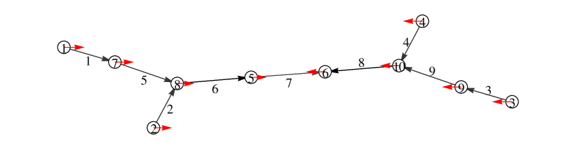
Fig. 5: The gray lines joining the buses show the magnitude of the power flow with the grayscale and the direction of the power flow with the arrows. Each line is numbered as shown. The red arrows at each bus show the oscillation mode shape; that is, the magnitude and direction of the entries of the right eigenvector $x_{{}_{\delta}}$ associated with the complex eigenvalue $\lambda_{3i}$. 1, 2, 3 and 4 are generator buses and 5 and 6 are load buses.

The power flow and oscillation for the base case is shown in Fig. 5 as well as the mode pattern of $\lambda_{3i}$. The mode pattern shows that area 1 is swinging against area 2.

Table 3: $\lambda_{3f}$ for redispatch from G1 to G3 in 10-bus system

​​​​Redispatch​​​​​​​​	Exact mode	Approximate mode
0.000	-0.038462 + 2.3832j	-0.038462 + 2.3832j
0.003	-0.038462 + 2.3785j	-0.038462 + 2.3786j
0.006	-0.038462 + 2.3738j	-0.038462 + 2.3739j
0.009	-0.038462 + 2.3691j	-0.038462 + 2.3692j
0.010	-0.038462 + 2.3675j	-0.038462 + 2.3676j
0.03	-0.038462 + 2.3350j	-0.038462 + 2.3357j
0.06	-0.038462 + 2.2829j	-0.038462 + 2.2858j
0.09	-0.038462 + 2.2262j	-0.038462 + 2.2331j
0.10	-0.038462 + 2.2061j	-0.038462 + 2.2149j
0.15	-0.038462 + 2.0947j	-0.038462 + 2.1173j
0.20	-0.038462 + 1.9586j	-0.038462 + 2.0060j
0.25	-0.038462 + 1.7810j	-0.038462 + 1.8735j
0.30	-0.038462 + 1.5152j	-0.038462 + 1.7005j

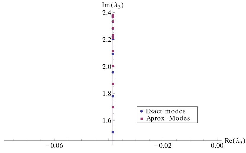
Fig. 6: Comparing the exact and approximate modes in the 10-bus system.

We examine changes in $\lambda_{3i}$ to test formula (97). Redispatch is made between generator 1 of area 1 and generator 3 of area 2. The generation of G1 is increased by an amount $r$ and the generation of G3 is decreased by $r$. Using formula (97), $d\lambda_{3}$ is computed for several values of $r$, then the approximate eigenvalue $\lambda_{3f}=d\lambda_{3}+\lambda_{3i}$ is calculated for every $r$. Table 3 shows $\lambda_{3f}$ for different steps of redispatch between G1 and G3 and compares the exact and approximate eigenvalues. Fig. 6 compares the exact and approximate eigenvalues of table 3 in the complex plane and Fig. 7 compares the exact and approximate imaginary part of the eigenvalues versus the redispatch. From table 3 we can confirm that formula (97) reproduces the first order variation of the eigenvalues with respect to the redispatch.

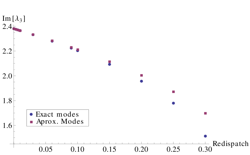
Fig. 7: Exact and approximate mode frequencies versus amount of redispatch in the 10-bus system.

11 6-bus system

In this section, we illustrate the use of formulas (9.2) and (9.2) in a simple 6-bus system. These formulas compute the sensitivity in the special case in which the voltage is considered constant at every bus. The loads are modeled with frequency dependence of real power. The bus data of the system is given in the table 4 and the data of the transmission lines is given in table 5.

Table 4: Bus data of the 6-bus system

bus	type	H (s)	D (s)	$P_{g}$	$P_{L}$
1	G	3.0	2.0	0.8	0.0
2	G	3.0	2.0	0.8	0.0
3	G	24.0	16.0	6.4	0.0
4	L	0.0	2.0	0.0	1.0
5	L	0.0	2.0	0.0	1.0
6	L	0.0	16.0	0.0	6.0

Table 5: Transmission line data of the 6-bus system

Line	$x$
1	0.45
2	0.45
3	0.0563
4	0.02
5	0.075

The system has two electromechanical modes. Table 6 shows the electromechanical eigenvalues of the system for the base case.

Table 6: Eigenvalues of the 6-bus system in the base case

				swing
	f (Hz)	$\zeta(\%)$	eigenvalue (rad/s)	profile
$\lambda_{1i}$	1.53802	1.81694	-0.175611 + 9.66364j	1,2$\leftrightarrow$3
$\lambda_{2i}$	1.72281	1.54097	-0.166826 + 10.8247j	1 $\leftrightarrow$ 2

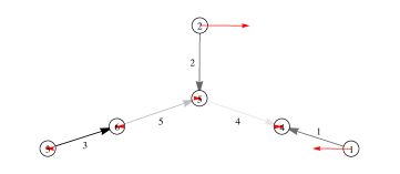
Fig. 8: Six-bus system: The gray lines joining the buses show the magnitude of the power flow with the grayscale and the direction of the power flow with the arrows. Each line is numbered as shown. The red arrows at each bus show the oscillation mode shape; that is, the magnitude and direction of the complex entries of the right eigenvector $x_{{}_{\delta}}$ associated to the critical complex eigenvalue $\lambda_{2i}$. Buses 1 and 2 are antinodes and buses 3,4,5,6 are nodes.

The power flow oscillation in the base case and the mode pattern of $\lambda_{2i}$ are shown in Fig. 8. The mode pattern shows that G1 is swinging against G2. The real coefficients $a_{{}_{rk}}$ and $a_{{}_{Ik}}$ in the equations (9.2) and (9.2) for the 6-bus system are shown in table 7.

Table 7: Coefficients $a_{{}_{rk}}$ and $a_{{}_{Ik}}$ for the 6-bus system

$a_{{}_{r1}}$	- 0.001346	$a_{{}_{I1}}$	- 0.70652
$a_{{}_{r2}}$	- 0.001275	$a_{{}_{I2}}$	- 1.13594
$a_{{}_{r3}}$	- 0.000055	$a_{{}_{I3}}$	- 0.006992
$a_{{}_{r4}}$	0.0	$a_{{}_{I4}}$	- 0.000351
$a_{{}_{r5}}$	0.0	$a_{{}_{I5}}$	- 0.001029

From table 7, coefficients related to the lines 1 and 2 are the biggest components of the vectors $a_{{}_{r}}$ and $a_{{}_{I}}$, but only the coefficients associated to the line 1 have the same sign, $a_{{}_{r1}}<0$ and $a_{{}_{I_{1}}}<0$. Line 1 connects generator G1, so it is clear from table 7 that increasing G1 helps to damp the oscillation. Fig. 9 shows the eigenvalue changes for redispatch between G1-G3, G1-G2, and G2-G3. When G1 (antinode) increases and G3 (node) decreases, $|\sigma_{2}|$ increases and $\omega_{2}$ decreases. If G1 decreases and G3 increases the effect is opposite. Any other combination of generators increases or decreases both the real and imaginary part of $\lambda_{2}$. Table 8 shows the values of $\lambda_{2f}=d\lambda_{2}+\lambda_{2i}$ for different steps of redispatch between G1 and G3. The damping is depicted in Fig. 10 as a function of the redispatch of active power. The damping ratio improves best when G1 increases and G3 decreases and when G2 increases and G3 decreases.

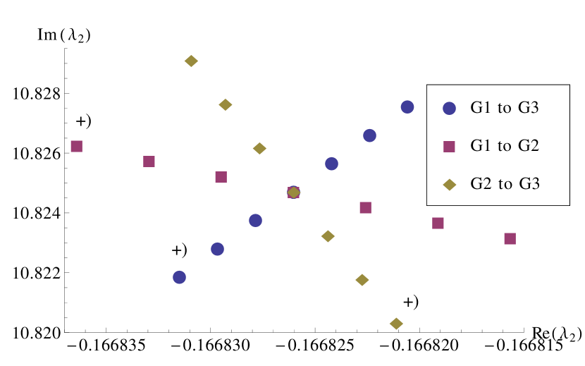
Fig. 9: Eigenvalues for redispatches of the 6-bus system.

Table 8: $\lambda_{2f}$ of redispatch G1 to G3 in the 6-bus system

Redispatch	$\lambda_{2f}$
0.009	-0.166830 + 10.8219j
0.006	-0.166830 + 10.8228j
0.003	-0.166828 + 10.8238j
0.0	-0.166826 + 10.8247j
-0.003	-0.166824 + 10.8257j
-0.006	-0.166822 + 10.8266j
-0.009	-0.166821 + 10.8276j

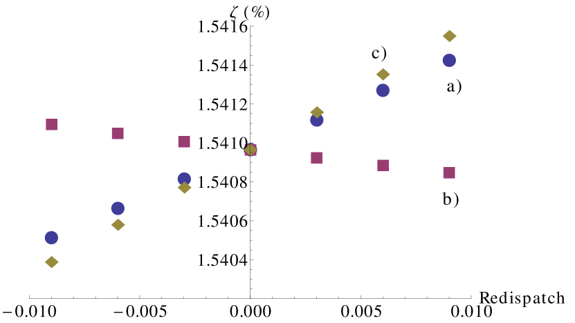
Fig. 10: Damping ratio versus redispatch   a) from G1 to G3, b) from G1 to G2, c) from G2 to G3.

12 Conclusions

We derive a new formula (97) for the sensitivity of oscillatory eigenvalues with respect to generator redispatch. The motivation is to understand and improve the damping of interarea oscillations with generator redispatch.

We use a power system dynamic model that expresses both real and reactive power flows and allows for variation of both angle and voltage magnitudes. The generator dynamics are a simple second order swing equation. The load modeling allows for frequency dependence and reactive power depending on voltage magnitude, but does not allow real power to depend on voltage magnitude. These modeling assumptions are the usual assumptions permitting energy function analysis of the power system, and in particular the network has a symmetric Laplacian. Indeed the derivation of the formula exploits the energy function structure. The hypothesis of the generator dynamic modeling is that there is some equivalent second order dynamic model for each generator that suffices for representing the wide-area oscillations, but that we do not need to know the parameters of each equivalent generator model. The formula (97) only includes the combined generator dynamics as a common factor that is the same for all redispatches.

In the past, there have multiple unsuccessful attempts to derive a formula with the properties of (97), and sometimes this derivation has been considered to be impossible. The combination of several ideas in this paper, some new and some old, enables the successful derivation of formula (97):

1. The new idea of working with the complex symmetric matrix form $x^{T}Qx$ (and not the more obvious Hermitian matrix form ${\bar{x}}^{T}Qx$).

2. New “line” coordinates $(\theta,\nu)$ for the angle differences and logarithm of the product of the voltages across the transmission lines. These new coordinates greatly simplify parts of the derivation.

3. Quadratic formulation of the eigenvalue problem. This formulation was recently applied to a power systems model by Mallada and Tang in [20].

4. The classical assumptions of lossless lines and no dependence of load real power on voltage magnitude that yield the energy function $R$ and a symmetric network Laplacian [2, 1, 23, 30, 25, 6].

The new formula (97) that describes the mode sensitivity has a factor $\alpha$ in the denominator that is the same for all generator redispatches, and $\alpha$ depends on the eigenvalue, the equivalent generator dynamics, and the modal eigenvector. Since the denominator of (97) is the same for all redispatches, to a large extent we can discriminate the effective redispatches by examining the effect of the redispatch on the numerator of (97).

The numerator of (97) expresses the changes in the mode in terms of the changes in angles across lines and load voltage magnitudes caused by the redispatch, with coefficients that depend on the mode shape and the base case power flows in the lines and the reactive power load demands. The base case power flows and the reactive power load demands are available from static state estimation. The mode shape is available from synchrophasor measurements, as discussed below. The new formula (97) is numerically verified in a 10 bus example in section 10.

Line coordinates $\theta$ that are the angle differences across the lines are discussed by Bergen and Hill in [2]. It is also known that it can be useful to divide the reactive power balance equations by the bus voltage magnitude, and use the logarithm of the bus voltage magnitudes, as, for example, in [24]. The line coordinates $(\theta,\nu)$ are a generalization that includes $\nu$ coordinates that describe the logarithm of the product of the voltage magnitudes associated with the lines, not the buses. The line coordinates not only greatly simplify the derivation of the formula, but are also expected to make the formula easier to interpret when it is applied. There are dependencies between the line coordinates in general meshed networks that are discussed in section 5.1.

The redispatch of real power naturally changes the pattern of real power flows and hence the angles across lines. Any reactive power flows caused by generator redispatch may also alter the voltage magnitude products across lines. The numerator of formula (97) identifies in which lines these changes in power flow is most effective.

The main emphasis of this paper is deriving formula (97). We have also begun to explore the implications and applications of (97) and we now indicate some initial conclusions.

1. In the case that the oscillatory mode has exactly zero damping, the formula predicts that, to first order, the generator redispatch changes only the mode frequency and not the mode damping. This suggests that generator redispatch could be more effective for maintaining sufficient damping than for emergency control when damping has vanished.

2. In the special case of considering real power dynamics only with constant voltage magnitudes, the formula (97) reduces to the remarkably simple form (250), in which changes in the mode depend on the changes in angles across lines caused by the redispatch, the real power flow in the lines, and the line angle coordinates of the mode shape eigenvector $x$.

3. The formula indicates which lines have suitable power flow and eigenvector components to affect oscillation damping. In particular, it is effective to use the redispatch to change the angle across lines that have both changes in the mode shape across the line and sufficient power flow in the right direction.

We note the following considerations and speculations towards implementing formula (97) to choose the generators to redispatch that are effective in maintaining suitable oscillation damping or damping ratio. The complex number $\alpha$ in the denominator of (97) that combines all the equivalent generator dynamics is common to all redispatches, so an approximate indication of the argument of $\alpha$ is probably all that is needed. The base case line power flows are known from the state estimator, and the load flow equations can be used to relate the generator redispatches to changes in the angles across lines and the load voltage magnitudes. The main remaining challenge is to determine the mode shape.

The mode shape is the quadratic eigenvector $x$ corresponding to $\lambda$ and it is easy to obtain from a conventional right eigenvector. The mode shape is in principle, and to some considerable extent in practice, available from ambient or transient synchrophasor measurements [29, 3, 10]. This is important since it is desirable to use measurements to minimize the use of poorly known dynamic power system models. Moreover, it is established [26, 33, 31, 18] that synchrophasors can make online measurements of the critical eigenvalue $\lambda$, the oscillatory mode frequency and damping. And, especially for the low frequency interarea modes, once the mode frequency is known, the mode might have a recurrent and fairly robust mode shape. Then it is conceivable that historical observations or offline computations or general principles about the mode shape could be used to augment or interpolate the real-time observations, or that the real time observations could be used to verify a predicted mode shape. Thus some combination of measurements and calculation from models could yield the mode shape needed to apply the formula to online calculations of optimum generation redispatch.

An alternative application of the formula is to use it to specify and justify heuristics for oscillation damping based on the mode shape and line power flows. This approach would similarly use a combination of measurements and calculation from models to obtain the mode shape, but one might expect that the approximate overall form of the mode shape might suffice. Our initial results suggest a basis for heuristics for redispatch based on changing the angles across lines with sufficient power flow and sufficient changes in the mode shape. These heuristics would be similar to heuristics for modal damping due to Fisher and Erlich [11, 12] that inspired our search for analytic patterns in modal damping, and we would like to confirm and refine these heuristics in future work.

More generally, for future work we will fully explore the implications and applications of the formula in order to realize its potential for controlling oscillation damping by generator redispatch. The formula could enable some combination of observations, computations and heuristics to more effectively damp interarea oscillations.

13 Acknowledgements

We gratefully acknowledge support in part from NSF grant CPS-1135825 and the Arend J. and Verna V. Sandbulte professorship. Sarai Mendoza-Armenta gratefully acknowledges support in part from Universidad Michoacana de San Nicolás de Hidalgo, Conacyt PhD Scholarship 202024. Ian Dobson gratefully acknowledge past support towards the solution of this problem coordinated by the Consortium for Electric Reliability Technology Solutions with funding provided in part by the California Energy Commission, Public Interest Energy Research Program, under Work for Others Contract No. 500-99-013, BO-99-2006-P. The Lawrence Berkeley National Laboratory is operated under U.S. Department of Energy Contract No. DE-AC02-05CH11231. Ian Dobson thanks Joe Eto for his support of long-term research.

Appendix: Jacobian and Quadratic Eigenstructure

In this appendix we show that the eigenvalues and eigenvectors of the quadratic form and the Jacobian of the system correspond. It is convenient to work with the full system of $2n-m$ equations, assumed to have balanced power injections, and without a reference bus. Then the system always has a mode with all angles increasing with a zero eigenvalue, which we can neglect.

To compute the eigenvalues of the system Jacobian, first we will change the second ordinary differential equations (19) to a set of first ordinary differential equations by defining the variable $\omega_{{}_{(2n-m)+i}}=\dot{\delta_{i}},\ i=1\ldots m$. Then the linearized equations become

$$\dot{\Delta z_{i}} =\Delta\omega_{{}_{(2n-m)+i}},\ i=1,\ldots m.$$ (A.1)

$$\dot{\Delta\omega}_{{}_{(2n-m)+i}} =-\frac{d_{i}}{m_{i}}\Delta\omega_{{}_{(2n-m)+i}}-\sum_{j=1}^{2n-m}\frac{L_{ij}}{m_{i}}\Delta z_{j},\ i=1,\ldots m.$$ (A.2)

$$0 =-\sum_{j=1}^{2n-m}L_{ij}\Delta z_{j},\ i=m+1,\ldots 2n-m.$$ (A.3)

Writing (A.1-A.3) in matrix form we have

$$\left(\begin{matrix}\dot{\Delta z^{d}}\\ 0\end{matrix}\right)=\left(\begin{matrix}J_{11}&J_{12}\\ J_{21}&J_{22}\end{matrix}\right)\left(\begin{matrix}\Delta z^{d}\\ \Delta z^{a}\\ \end{matrix}\right),$$ (A.4)

where $z^{d}$ is a vector of size $2m$ composed by the dynamical variables of the system, and $\Delta z^{a}$ is a vector of size $2(n-m)$ composed of the algebraic variables.

The differential algebraic system can be reduced to a purely differential system by expressing the algebraic variables in terms of the dynamic variables and substituting them in the system. This leads to $\Delta z^{a}=-J^{-1}_{22}J_{21}\Delta z^{d}$ and the linearization of the reduction

$$\dot{\Delta z^{d}}=J_{red}{\Delta z^{d}},$$ (A.5)

where $J_{red}=J_{11}-J_{12}J^{-1}_{22}J_{21}$. Once the system is reduced, the symmetry of the Laplacian of the system is destroyed.

To avoid the reduction (A.5), it is better to work directly with the differential-algebraic equations [28]. (A.4) can be written as a singular ordinary differential equation system

$$E\left(\begin{matrix}\dot{\Delta z^{d}}\\ \dot{\Delta z^{a}}\end{matrix}\right)=J\left(\begin{matrix}\Delta z^{d}\\ \Delta z^{a}\end{matrix}\right),\quad\text{where}\quad E=\left(\begin{matrix}I&0\\ 0&0\end{matrix}\right).$$ (A.6)

To find the eigenvalues associated with (A.6), the generalized eigenvalue problem has to be solved; i.e., $\mu Ev=\gamma Jv$. The eigenvalues $\lambda$ are defined as $\lambda=\frac{\mu}{\gamma}$. If $\gamma=0$, the eigenvalue $\lambda$ is regarded as infinite. The infinite eigenvalues arise from the singularity of the $E$ matrix.

For the finite eigenvalues of the Jacobian, we can write $Jv=\lambda Ev$. The eigenvector $v$ is $v=(v^{d},v^{a})$, where the size of the vector $v^{d}$ is the number of dynamics variables ($z^{d}$), and the size of $v^{a}$ is the number of algebraic variables. It has been proved [28] that for any triple $(\lambda,v^{d},v^{a})$ that satisfies (A.6), the pair $(\lambda,v^{d})$ satisfies (A.5). Conversely if $(\lambda,v^{d})$ satisfies the reduced system, then $(\lambda,v^{d},v^{a})$ satisfies the complete system with $v^{a}=-J^{-1}_{22}J_{21}v^{d}$, so the finite eigenvalues of $J$ are the modes of the system.

Now we will prove that the finite eigenvalues of $J$ are finite eigenvalues of $Q$. Let $v$ be an eigenvector associated with the finite eigenvalue $\lambda$; that is, $Jv=\lambda E$. Then, from (A.1-A.3),

$$\lambda v_{i} =v_{(2n-m)+i}$$ (A.7)

$$\lambda v_{(2n-m)+i} =-\frac{d_{i}}{m_{i}}v_{(2n-m)+i}-\sum_{j=1}^{2n-m}\frac{L_{ij}}{m_{i}}v_{j}$$ (A.8)

$$0 =-\sum_{j=1}^{2n-m}L_{ij}v_{j}.$$ (A.9)

Using (A.7) in (A.8), and multiplying by $m_{i}$,

$$\lambda^{2}m_{i}v_{i}+\lambda d_{i}v_{i}+\sum_{j=1}^{n+m}L_{ij}v_{j} =0$$ (A.10)

$$\sum_{j=1}^{n+m}L_{ij}v_{j} =0.$$ (A.11)

But (A.10)-(A.11) is (21). Then the eigenvector $x$ of the quadratic eigenvalue problem with finite eigenvalue $\lambda$ corresponds exactly to the eigenvector $v=(\lambda x_{g},x)$ of $J$, where $x_{g}$ is the vector of components of $x$ corresponding to the generator angles.

References

[1] A. Arapostathis, S.S. Sastry, P. Varaiya,
IEEE Trans. Circuits and Systems, vol CAS-29, no. 10, October 1982, pp. 673-679.
[2] A.R. Bergen, D.J. Hill, A structure preserving model for power systems stability analysis, IEEE Trans. Power App. Syst., vol. PAS-101, pp. 25-35, Jan. 1981.
[3] N.R. Chaudhuri, B. Chaudhuri, Damping and relative mode-shape estimation in near real-time through phasor approach, IEEE Trans. Power Syst., vol. 26, no. 1, pp. 364-373, Feb. 2011.
[4] C.Y. Chung, L. Wang, F. Howell, P. Kundur,
Generation rescheduling methods to improve
power transfer capability constrained by
small-signal stability,
IEEE Trans. Power Syst., vol. 19, no. 1, pp. 524-530, Feb. 2004.
[5] Cigré Task Force 07 of Advisory Group 01 of Study Committee 38,
Analysis and control of power system oscillations, Paris, December 1996.
[6] C. L. DeMarco, J. J. Wassner, A generalized
eigenvalue perturbation approach to coherency, Proc. IEEE
Conference on
Control Applications, Albany, NY, September 1995, pp. 605-610.
[7]
R. Diao, Z. Huang, N. Zhou, Y. Chen, F. Tuffner, J. Fuller, S. Jin, J.E Dagle,
Deriving optimal operational rules for mitigating inter-area oscillations,
Power Systems Conference and Exposition, Phoenix AZ USA, March 2011.
[8] I. Dobson, Fernando Alvarado, C. L. DeMarco, Sensitivity
of Hopf bifurcations to power system parameters, Proceedings of the 31st
Conference on Decision and Control, Tucson, Arizona, December 1992.
[9] I. Dobson, F.L. Alvarado, C.L. DeMarco, P. Sauer, S. Greene, H. Engdahl, J. Zhang,
Avoiding and suppressing oscillations,
PSerc publication 00-01, December 1999.
[10] L. Dosiek, N. Zhou, J.W. Pierre, Z. Huang, D.J. Trudnowski,
Mode shape estimation algorithms under ambient conditions: A comparative review,
IEEE Transactions on Power Systems, vol. 28, no. 2,
May 2013, pp. 779-787.
[11] A. Fischer, I. Erlich, Assessment of power
system small signal stability based on mode shape information,
IREP Bulk Power System Dynamics and Control V,
Onomichi, Japan, Aug 2001.
[12] A. Fischer, I. Erlich, Impact of
long-distance power transits on the dynamic security of
large interconnected power systems,
IEEE Porto Power Tech Conference,
Porto, Portugal, September 2001.
[13] M. Jonsson, M. Begovic, J. Daalder,
A new method suitable for real-time
generator coherency determination,
IEEE Transactions on Power Systems, vol. 19, no. 3,
August 2004, pp. 1473-1482.
[14] Z. Huang, N. Zhou, F. Tuffner, Y. Chen, D. Trudnowski, W. Mittelstadt, J. Hauer, J. Dagle,
Improving small signal stability through operating point
adjustment, IEEE PES General Meeting,
Minneapolis, MN USA, July 2010.
[15] Z. Huang, N. Zhou, F.K. Tuffner, Y. Chen, D.J. Trudnowski, MANGO - Modal Analysis for Grid Operation:
A method for damping improvement through operating point adjustment,
Prepared for the U.S Department of Energy
October, 2010.
[16] IEEE Power system engineering committee,
Eigenanalysis and frequency domain
methods for system dynamic performance,
IEEE Publication 90TH0292-3-PWR, 1989.
[17]
IEEE Power Engineering Society Systems Oscillations Working Group,
Inter-area oscillations in power systems, IEEE Publication 95 TP 101,
October 1994.
[18] IEEE Task Force on Identification of Electromechanical Modes,
Identification of electromechanical modes in power systems,
IEEE Special Publication TP462,
June 2012.
[19] M. Klein, G.J. Rogers, P. Kundur,
A fundamental study of inter-area oscillations in power systems,
IEEE Transactions on Power Systems, vol. 6,
no. 3, August 1991, pp. 914-921.
[20] E. Mallada, A. Tang, Improving damping of power networks: power scheduling and impedance adaptation,
50th IEEE Conference on Decision and Control and European Control Conference (CDC-ECC),
Orlando, FL, USA, December 2011.
[21] S. Mendoza-Armenta, Analysis of degenerate and interarea oscillations in electric power systems, (in Spanish),
PhD thesis, Instituto de Física y Matemáticas, Universidad Michoacana, Morelia, Michoacán, México, to appear in 2013.
[22] H.K. Nam, Y.K. Kim, K.S. Shim, K.Y. Lee, A new eigen-sensitivity theory of augmented matrix and its applications to power system stability, IEEE Trans. Power Systems, vol. 15, pp. 363-369, Feb. 2000.
[23]
N. Narasimhamurthi and M. T. Musavi, A general energy function for transient stability of power systems, IEEE Trans. Circuits and Systems., vol. CAS-31, pp. 637-645, July 1984.
[24]
T.J. Overbye, I. Dobson, C.L. DeMarco,
Q-V Curve interpretations of energy
measures for voltage security,
IEEE Transactions on Power Systems,
vol. 9, no. 1, Feb. 1994, pp. 331-340.
[25] M. A. Pai, Energy Function Analysis for Power System Stability,
Kluwer Academic Publishers, Boston, 1989.
[26] J.W. Pierre, D.J. Trudnowski, M.K. Donnelly,
Initial results in electromechanical mode identification from
ambient data,
IEEE Transactions on Power Systems, vol. 12,
no. 3, August 1997, pp. 1245-1251.
[27] G. Rogers, Power System Oscillations, Kluwer Academic, 2000.
[28] T. Smed, Feasible eigenvalue sensitivity for large
power systems, IEEE Transactions on Power Systems, Vol. 8, No. 2,
May 1993, pp. 555-563.
[29] D.J. Trudnowski, Estimating electromechanical mode shape from synchrophasor measurements, IEEE Trans. Power Syst., vol. 23, no. 3, pp. 1188-1195, Aug. 2008.
[30] N.K. Tsolas, A. Arapostathis, P.P. Varaiya, A structure preserving energy function for power system transient stability analysis,
IEEE Trans. Circuits and Systems, vol. CAS-32, no. 10, October 1985, pp. 1041-1049.
[31] L. Vanfretti, J.H. Chow,
Analysis of power system oscillations for developing synchrophasor data applications,
2010 IREP Symposium - Bulk Power System Dynamics and Control VIII, Buzios, Brazil, August 2010,
[32] Shao-bu Wang, Quan-yuan Jiang, Yi-jia Cao,
WAMS-based monitoring and control of Hopf bifurcations in multi-machine power systems,
Journal of Zhejiang University Science A, vol. 9, no. 6, pp. 840-848, 2008.
[33] R.W. Wies, J.W. Pierre, D.J. Trudnowski,
Use of ARMA block processing for estimating
stationary low-frequency electromechanical modes
of power systems,
IEEE Trans. Power Syst., vol. 18, no. 1, Feb. 2003, pp. 167-173.