The 4-Body Problem in a (1+1)-Dimensional Self-Gravitating System

A. Lauritzen, P. Gustainis, and R.B. Mann
Dept. of Physics & Astronomy, University of Waterloo Waterloo, ONT N2L 3G1, Canada
PACS numbers: 04.40.-b, 04.25.-g, 05.45.Ac, 04.20.Jb

We report on the results of a study of the motion of a four particle non-relativistic one-dimensional self-gravitating system. We show that the system can be visualized in terms of a single particle moving within a potential whose equipotential surfaces are shaped like a box of pyramid-shaped sides. As such this is the largest $N$-body system that can be visualized in this way. We describe how to classify possible states of motion in terms of Braid Group operators, generalizing this to $N$ bodies. We find that the structure of the phase space of each of these systems yields a large variety of interesting dynamics, containing regions of quasiperiodicity and chaos. Lyapunov exponents are calculated for many trajectories to measure stochasticity and previously unseen phenomena in the Lyapunov graphs are observed.

1 Introduction

One of the oldest problems in physics is that of determining the motion of $N$ bodies under a specified mutual force. Commonly referred to as the $N$-body problem, it occurs frequently in many distinct subfields and remains an active area of research.  When the specified interaction is gravitation the problem is particularly interesting, partly because of obvious astrophysical applications and partly because some basic issues in the statistical behaviour of such systems are still not well-understood.

One-dimensional self-Gravitating Systems (OGS’s) continue to play an important role in this regard.  Even in the simplified setting of one spatial dimension, there are still many open questions about the OGS concerning its ergodic behaviour, the conditions (if any) under which equipartition of energy is attained, and whether or not it can reach a true equilibrium configuration from arbitrary initial conditions. Furthermore, even for non-relativistic (Newtonian) gravity, OGS’s have proven to be very useful in modeling many diverse physical systems. Stable core-halo structures have been shown to exist in the OGS phase-space that are reminiscent of those found in globular clusters [1], in which a dense core of particles near equilibrium are surrounded by a cloud of particles with high kinetic energy that interact very weakly with the core. The OGS also models the motion of stars interacting with a highly flattened galaxy [2] and the dynamics of flat, parallel sheets colliding along a perpendicular axis [3]. A preliminary study of the relativistic case yielded a complete derivation of the partition and single-particle distribution functions in both the canonical and microcanonical ensembles to leading order in a post-Newtonian expansion [4].  Recently non-relativistic OGS’s have been shown to exhibit a new phase of evolution in which fractal spatial structure emerges from non-fractal initial conditions [5].

Even for small values of $N$, OGS’s exhibit interesting novel behaviour and model interesting physical systems. The 3-body OGS is equivalent to a system of two elastically colliding billiard balls in a uniform, gravitational field [6], as well as to a bound state of three quarks to form a “linear baryon” [7].  It can be extended to fully include relativistic gravitational interactions [8], and investigations have been carried out for both the equal mass [9] and unequal mass [10] cases .  Furthermore, it is isomorphic to a system in which a billiard elastically collides with a wedge of fixed angle in a uniform, gravitational field [3].  As such, one can study the 3-body OGS (non-relativistically and relativistically) by studying the motion of a single particle moving in two spatial dimensions in a specified potential.  The motion in this case is readily visualizable, and the different types of motion can be classified into three categories: annulus, where each particle always crosses the other two in succession; pretzel, in which two particles cross each other at least twice in a row before either crosses the third; and chaotic, where the sequence of particle crossings does not progress in a discernible pattern.

In this paper we carry out an investigation of the 4-body OGS. Analogous to its 3-body counterpart, this system is isomorphic to the motion of a single particle moving in three spatial dimensions in a specified potential.  Consequently the 4-body case is of particular interest in that it is the largest value of $N$ for which the motion of the system can be directly visualized (we note that evidence has been provided that when $N\geqq 11$ there is no segementation of the phase space and the system is ergodic [11]).  We consider only the non-relativistic case (which to our knowledge has never been studied), leaving the relativistic case for future work.

The outline of our paper is as follows. We begin with an overview of the problem of 4-body motion in Newtonian gravity, and describe a general classification scheme for the motion of the particles that is an extension of that employed in the 3-body case [9].   Two numerical solution methods employed in the paper are described: the first using numerical integration and the equations of motion to obtain smooth particle trajectories. The second method uses collisions between particles as time steps and maps between the collisions, providing a means to analyze trajectories and accurately calculate Lyapunov exponents at very large time scales. Utilizing two solution methods also provided a useful cross check for results obtained. We then specify to a system of equal masses, and describe sample trajectories of various dimensionality.  Following this we present a proposal for constructing Poincare plots for the various trajectories encountered in this system. These plots are three-dimensional generalizations of the two-dimensional plots constructed for the three-body case [3]. Although difficult to visualize in complete generality, they do provide interesting information concerning the chaotic behaviour of the system. We also analyze the Lyapunov exponents for the system we consider to obtain measures of stochasticity. The analysis was done using a method due to Benettin et.al.[16] for calculating the largest Lyapunov exponent. These results are very consistent with what would be expected from the plots from qualitative assessment of the stochasticity of the different trajectories. We find as well an unexpected feature of some Lyapunov graphs where the perturbed and unperturbed trajectories diverged significantly from one another. We refer to this effect as orbital bifurcation, and find that it is caused by small changes in the collision order between the two trajectories, ultimately leading to large differences in their qualitative behaviour. We then close our paper with some concluding remarks.

2 Four-Body Motion in Newtonian Gravity

In (1+1) dimensional Newtonian gravity, the Hamiltonian of our system of particles is given by:

$$H=\sum_{a=1}^{4}\frac{p_{a}^{2}}{2m_{a}}+\pi G\sum_{a=1}^{4}\sum_{b=1}^{4}m_{a}m_{b}\left|z_{a}-z_{b}\right|$$ (1)

which is simply the sum of the kinetic energies of the particles and the potential interactions between them. The gravitational potential is determined from

$$\nabla^{2}\phi=4\pi G\rho=4\pi G\sum_{a=1}^{4}m_{a}\delta(x-z_{a})$$ (2)

where $\rho$ is the mass density of the system, here modeled as a set of four point particles. In one spatial dimension the solution to this equation is

$$\phi\left(x\right)=2\pi G\sum_{a=1}^{4}m_{a}\left|x-z_{a}\right|$$ (3)

and the potential is given by $V=\frac{1}{2}\sum_{a=1}^{4}m_{a}\phi\left(z_{a}\right)$. The equations of motion are given by:

$$\dot{z}_{a}=\frac{\partial H}{\partial p{{}_{a}}},\qquad\dot{p}_{a}=-\frac{\partial H}{\partial z{{}_{a}}}$$ (4)

Since the momentum is conserved and since the potential depends only on the separations between the particles, there are actually only six independent degrees of freedom in the 4-body system: the three separations between the particles and their conjugate momenta.  This is easily seen by making the following convenient change of coordinates

$$\begin{array}[]{cc}z_{12}=\sqrt{2}\rho&z_{34}=\sqrt{2}\alpha\\ z_{13}=\frac{1}{\sqrt{2}}(\rho+\sqrt{3}\beta-\alpha)&z_{23}=\frac{1}{\sqrt{2}}(-\rho+\sqrt{3}\beta-\alpha)\\ z_{24}=\frac{1}{\sqrt{2}}(-\rho+\sqrt{3}\beta+\alpha)&z_{14}=\frac{1}{\sqrt{2}}(\rho+\sqrt{3}\beta+\alpha)\end{array}$$ (5)

where $z_{ij}=z_{i}-z_{j}$.  The conjugate momenta are given by

$$\begin{array}[]{cc}p_{1}=\frac{1}{\sqrt{2}}(p_{\rho}+\frac{\sqrt{3}}{2}p_{\beta})&p_{2}=\frac{1}{\sqrt{2}}(-p_{\rho}+\frac{\sqrt{3}}{2}p_{\beta})\\ p_{3}=\frac{1}{\sqrt{2}}(p_{\alpha}-\frac{\sqrt{3}}{2}p_{\beta})&p_{4}=\frac{1}{\sqrt{2}}(-p_{\alpha}-\frac{\sqrt{3}}{2}p_{\beta})\end{array}$$ (6)

where we have set $p_{1}+p_{2}+p_{3}+p_{4}=0$ by conservation of momentum.  Without loss of generality the centre of mass of the system can be fixed at the origin. The reason for this choice of coordinate transformation is to produce a symmetric potential in 3 spatial dimensions. It can be obtained by requiring that it reduce to the more familiar 3-body-like potential [6] when two particles are placed directly on top of one another (i.e. when one of $z_{12}$, $z_{23}$, or $z_{13}$ vanish).

In the equal mass case the Hamiltonian (1) becomes

$$H =\frac{1}{2m}(p_{\rho}^{2}+p_{\alpha}^{2}+\frac{3}{2}p_{\beta}^{2})+\frac{8\pi Gm^{2}}{\sqrt{8}}\left[\left|\rho\right|+\left|\alpha\right|+\frac{1}{2}\left|\rho+\alpha+\sqrt{3}\beta\right|\right.$$

$$\left.+\frac{1}{2}\left|\rho-\alpha+\sqrt{3}\beta\right|+\frac{1}{2}\left|\rho+\alpha-\sqrt{3}\beta\right|+\frac{1}{2}\left|\rho-\alpha-\sqrt{3}\beta\right|\right]$$ (7)

which is the Hamiltonian of a single particle moving in three spatial dimensions in a linear potential whose shape is that of a 3-simplex.  In general a the $N$ particle OGS can be mapped to a single particle moving in $N-1$ dimensions in a linear potential whose equipotential surfaces are that of an $N-1$ simplex.  As such, the 4-body OGS is the largest system for which the motion can be directly visualized.  We shall refer to the form (7) as the Hamiltonian of the box-particle.

Using this result, plot the potential in the equal mass case from equation (7), defined as

$$V(\rho,\beta,\alpha)=H(p_{\rho}=0,p_{\beta}=0,p_{\alpha}=0)$$ (8)

which can be drawn in $(\rho,\beta,\alpha)$ space as shown in Figure 1. An equipotential surface is that of a cube of pyramid-shaped sides.  A cross-section of this surface through any of the edges of one of these pyramids yields a hexagon whose sides are not all of equal length. This is reflective of the fact that on such cross-sections the problem reduces to that of the three-body problem with unequal masses [10] since two particles occupy the same position.

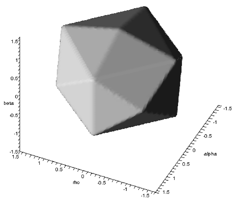
Figure 1: Shape of the Newtonian potential in the equal mass case, for a certain value of $V$.  Larger values of $V$ will produce larger scaled “boxes”.

2.1 Methods for Solving the Equations of Motion

We turn now to the problem of solving the equations of motion (4). As there are no singularities in the potential whenever two particles cross, we assume that the particles pass through each other freely upon collision.   Prior to any collision, solving the equations is trivial: since the acceleration of each particle is constant at any given instant, the trajectory of each particle is a quadratic function of time. However after each subsequent crossing the acceleration of a given particle changes its magnitude, since the number of bodies to the right and left of it have changed.  Hence an analytic closed-form solution to the equations of motion (4) is completely impractical.

We therefore solve the equations of motion numerically, using a Matlab ODE (ordinary differential equation) routine to integrate the equations of motion (4).  For the most part the standard “ode45” routine proved to be completely sufficient for our needs.  In some cases we also used the “ode113” routine because of our extremely stringent error tolerances ($10^{-9}$ relative and $10^{-10}$ absolute).  The former is based on the Runge-Kutta formula while the latter is a variable order Adams-Bashforth-Moulton PECE solver (see the Matlab ODE documentation for more detail and references). This solution method was very useful for mapping the Lissajous figures and particle trajectories along smooth paths, allowing one to see trajectory patterns, such as annulus and pretzel, more clearly.

Integration of the equations of motion is not sufficient for computation of the largest Lyapunov exponents, and so we employed a different solution method. The differential equation solver yields numerical errors that are negligible on the smaller time scales used for mapping trajectories and Poincare plots. However, when analyzing Lyapunov exponents, very large time scales are required to obtain reliable asymptotic behaviour. Numerical errors from the differential equation solver cause Lyapunov graphs to diverge after only a few hundred time steps. We therefore compute the trajectories from collision to collision, a feasible problem that can can be solved in closed form because all particles follow paths of constant acceleration in between collisions. Using this method, such numerical divergences are avoided and stable Lyapunov graphs can be obtained.

As a cross-check on our methods, we find that the Lissajous plots are very similar and Poincare plots precisely the same between the two methods. This is confirmed through careful analysis of the Lissajous figures. As will be seen, the dimensions of the figures are the same and the features, such as the bands and stripes, seen clearly on the collision method plots, are shared between plots from the two methods. Furthermore, the Poincare plots can be matched point-to-point between the two methods, further confirming that the solution methods are equivalent (these are not shown for simple reasons of redundancy).

We employ two methods of analysis.  One is that of plotting the trajectories of the box-particle in $(\rho,\beta,\alpha)$ space for a variety of initial conditions. We also plot the motions of the four particles as a function of time for each case.  This provides an alternate means of visualizing the difference between various types of motions that can arise in the system.

To perform the numerical analysis we rescale the variables to have dimensionless values

$$p_{i}=M_{tot}c\hat{p_{i}}\qquad z_{i}=\frac{4}{\kappa M_{tot}c^{2}}\hat{z_{i}}$$ (9)

where $M_{tot}=4m$ is the total mass of the system and $\hat{p_{i}}$ and $\hat{z_{i}}$ are the dimensionless momenta and positions respectively.  The dimensionless mass and Hamiltonian are:

$$\eta=\frac{H}{M_{tot}c^{2}}\qquad\hat{m_{i}}=\frac{m_{i}}{M_{tot}}$$ (10)

Using the dimensionless variables in (9) and (10), the Hamiltonian (1) becomes:

$$\eta=\sum\limits_{a=1}^{4}\frac{\hat{p_{a}^{2}}}{2\hat{m_{a}}}+\frac{1}{2}\sum\limits_{a=1}^{4}\sum\limits_{b=1}^{4}\hat{m_{a}}\hat{m_{b}}\left|\hat{z_{a}}-\hat{z_{b}}\right|$$ (11)

As for the equations of motion (4) one gets:

$$\frac{\partial\eta}{\partial\hat{p_{i}}} = \frac{d\hat{z}_{i}}{d\hat{t}}$$ (12)

$$\frac{\partial\eta}{\partial\hat{z_{i}}} = -\frac{d\hat{p_{i}}}{d\hat{t}}$$ (13)

where $t=\frac{4c}{8\pi GM_{tot}}\hat{t}$.

A time step in the numerical code has a value $\hat{t}=1$.  All the numerical calculations were carried out using the rescaled variables (9).  Henceforth we drop all of the “hats” of the dimensionless variables for convenience.

Note that since the energy is a constant of the motion, we could further rescale all quantities in terms of $\eta$, thereby fixing this final redundant scale. However we shall find it convenient to employ the above rescalings, as it affords us more freedom in choosing initial conditions.

2.2 Classifying the Motions

Prior to any collision between the particles the evolution of the system is straightforward: each particle moves with a constant acceleration that is proportional to the difference between the total mass on its right and left sides.  However after a collision, where we assume that the particles pass through each other, the mass difference changes, and with it the accelerations of the particles.  It is these repeated changes in the accelerations of the particles that yield the interesting dynamics of the system.

From the perspective of the box particle, such crossings correspond to the box particle crossing any plane that bisects the 3-simplex through its vertices and edges, yielding a discontinuous change in the box particle’s acceleration. These planes occur in pairs whose line of intersection is along each of the three principal axes, for a total of six such planes. Their equations are given by setting any one of the six quantities in eq. (5) to zero, and each plane corresponds to the crossing of a pair of particles. For example $\rho=0$ corresponds to the crossing of particles 1 and 2, whereas $\rho=\sqrt{3}\beta+\alpha$ corresponds to the crossing of particles 2 and 4.

Initially we have all of the crossings listed in order as a string of vanishing quantities. $\{z_{12}z_{13}z_{14}z_{23}z_{24}z_{34}\}$. The direction of crossing is irrelevant; for example 1 crossing 2 is equivalent to 2 crossing 1.  At any given instant we can fix the positions of particles in a certain order from left to right, i.e. $(1,2,3,4)$, in which case we only have 3 possible crossings: $\{z_{12},z_{23},z_{34}\}$.  We denote these using the Braid operators $\{\sigma_{1},\sigma_{2},\sigma_{3}\}$, with $\sigma_{1}$ corresponding to an interchange between the right-most pair of particles, $\sigma_{2}$ for the middle pair and $\sigma_{3}$ for the left-most pair. More generally, instead of defining the actual particles as $(1,2,3,...)$, we define the positions as that sequence: the left-most particle is at position $1$, next $2$, and so on with the right-most particle being at position $N$. Given any sequence of particle crossings, we can employ Braid Group notation [12, 13] to classify the motion, denoting pair crossings with the set $\{\sigma_{1},\sigma_{2},\ldots,\sigma_{N-1}\}$. For example the sequence $z_{12}z_{13}z_{23}z_{14}z_{24}...$ is described by $\sigma_{1}\sigma_{2}\sigma_{1}\sigma_{3}\sigma_{2}$, and the initial configuration $(1,2,3,4)$ becomes the final configuration $(3,4,2,1)$.  Since crossing direction is irrelevant, the reciprocal notation for the Braid Group is ignored (i.e. $\sigma_{j}=\sigma_{j}^{-1}$  in this context). We do not concern ourselves with the permutation properties of the braid groups. We use this notation out of convenience in classifying the sequence of motion of the particles. Since the particular sequence of collision is important, any permutation of the operators would result in loss of information about the motion in the system.  

We are now ready to classify the distinct kinds of motion that can occur. Consider first the 3-body case. This problem can be mapped to that of a single particle moving in a hexagonal-shaped well, with the bisectors of the hexagon denoting pair-crossings of the particles [9]. In this case we have $\{\sigma_{1},\sigma_{2}\}$ as the Braid operators.  For any string of these we can classify the motion in the equal mass case as follows:

$$\begin{array}[]{cc}\sigma_{1}\sigma_{1}\;,\;\sigma_{2}\sigma_{2}&\text{A motion}\\ \sigma_{1}\sigma_{2}\;,\;\sigma_{2}\sigma_{1}&\text{B motion}\end{array}$$ (14)

by comparing subsequent items in the string; we have included the $A/B$ descriptors employed previously in 3-body studies [9].  In other words, since crossing direction is irrelevant, the only interesting types of motion are when the same pair of particles crosses twice in a row ($A$-motion) corresponding to crossing a single bisector of the hexagon twice in succession, or when one particle crosses each of its compatriots in succession ($B$-motion) corresponding to the crossing of two successive bisectors.  In the unequal mass case the hexagon is no longer symmetric, and so $\sigma_{1}\sigma_{1}$, say, is now distinguishable from $\sigma_{2}\sigma_{2}$.  However one could impose an equivalence relation between these two motions and continue to employ the above notation.  Any given motion in the system can be characterized by a sequence of letters $A$ and $B$ (called a symbol sequence), with a finite exponent $n$ denoting $n$-repeats and an over-bar denoting an infinite repeated sequence.

This idea extends naturally to the 4-body system. Here the Braid operators are $\{\sigma_{1},\sigma_{2},\sigma_{3}\}$.  We can construct the following definitions:

$$\begin{array}[]{cc}\sigma_{1}\sigma_{1}\;,\;\sigma_{2}\sigma_{2}\;,\;\sigma_{3}\sigma_{3}&\text{A motion}\\ \sigma_{1}\sigma_{2}\;,\;\sigma_{2}\sigma_{1}\;,\;\sigma_{2}\sigma_{3}\;,\;\sigma_{3}\sigma_{2}&\text{B motion}\\ \sigma_{1}\sigma_{3}\;,\;\sigma_{3}\sigma_{1}&\text{C motion}\end{array}$$ (15)

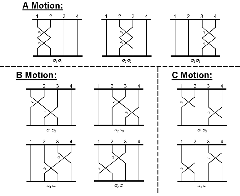
Figure 2: 4-body motion classes.

whose results can be visualized in Figure 2. The $A$ and $B$ motions still represent the same physical situations as in the 3-body case. However there is now a new type of motion: $C$ motion, which is when two particles cross one another and then the other two cross one another.

We can proceed further, generalizing our arguments and definitions to the $N$-body case and make a more formal definition of our motion classes whose specific cases for $N=3$ and $N=4$ will be equivalent to what we have described above.

To describe crossings of $N$ particles for a specific trajectory we have the Braid operators $\{\sigma_{1},\sigma_{2},\ldots,\sigma_{N}\}$.  A sequence of $m$ pair crossings will be described by

$$\sigma_{f(1)}\sigma_{f(2)}\sigma_{f(3)}...\sigma_{f(m)}$$ (16)

where $1\leq f(x)\leq(N-1)$ for all $1\leq x\leq m$ is a discrete integer function .  Here $\sigma_{f(x)}$ means that the particles currently in positions $f(x)$ and $f(x)+1$ cross.  Any given sequence of $m$ Braid operators forms a unique ordered list of crossings for the given trajectory.  As stated previously, crossing directions are irrelevant.

Now we define a new function

$$g(x)\equiv|\Delta f(x)|=|f(x+1)-f(x)|$$ (17)

using the finite forward difference function of $f$ [14]. We are interested in the absolute difference between subsequent terms, and thus we have $0\leq g(x)\leq(N-2)$ for all $1\leq x\leq(m-1).$ Now $g(x)$ defines a metric that describes the relative “distance” between any pair of crossings, and we classify the motion according to this distance

$$\begin{array}[]{cc}g(x)&\text{Motion Class}\\ 0&A\\ 1&B\\ 2&C\\ ..\end{array}$$ (18)

denoting each type by increasing letters of the alphabet. In other words, $A$-motion corresponds to any 2 crossings in nearest proximity – two particles cross each other twice in succession.  $B$-motion corresponds to any 2 crossings in next-nearest proximity – two particles cross each other, and then one of them crosses its other nearest neighbour.  $C$-motion corresponds to any 2 crossings in next-to-next-nearest proximity: two particles cross each other and then a neighbouring pair cross each other.  We can continue on in this fashion until we reach the extreme case in which the right-most pair of particles cross one another followed by the crossing of the left-most pair (or vice-versa).

We illustrate this classification with some examples. For $N=3$, we have $1\leq f(x)\leq 2$.  Suppose we have a crossing sequence $\sigma_{1}\sigma_{2}\sigma_{1}\sigma_{1}\sigma_{2}$, yielding from (14) the symbol sequence $BBAB$. By our definition above we have

$$\begin{array}[]{cccccc}x&1&2&3&4&5\\ f(x)&1&2&1&1&2\\ g(x)&1&1&0&1\end{array}$$ (19)

and from (18) we get $BBAB$ as we expected.  For $N=4$, we have $1\leq f(x)\leq 3$.  Consider the previous example $\sigma_{1}\sigma_{2}\sigma_{1}\sigma_{3}\sigma_{2}$, which from (15) yields the symbol sequence $BBCB$, the same result we would obtain from computing successive values of $g(x)$ (which are $1,1,2,1$ for this example).

The preceding classification system is limited to pair-wise crossings and does not cover situations in which more than one pair of particles crosses at the exact same time step.  While the braid group notation does allow for multiple collisions by writing them “left-to-right”, it is important in our system whether or not these collisions occur at the same time step.  For the $N$-body problem, a simultaneous collision of $m$ particles corresponds to the crossing of a single particle through an $(N-m)$-dimensional surface in the interior of the $(N-1)$ simplex.  This surface is obtained by continually bisecting the simplex along its (higher-dimesional) edges and vertices until the surface of appropriate dimensionality is obtained.  We can denote such collisions by extending the braid group notation with the set $\{\sigma_{1^{m}},\sigma_{2^{m}},\ldots,\sigma_{(N+1-m)^{m}}\}$, where the subscript denotes which set of particles is involved, beginning with the left-most, and the superscript (on these subscripts) denotes the number of particles in the collision.  For example $\sigma_{9^{7}}$ denotes a 7-particle collision that involves particles 9-15.  We shall drop the superscript “2” when pair-wise collisions are involved. All collisions yield crossings except for the situation in which the initial conditions cause $m$ particles to occupy the same point throughout the motion.  In this latter case the system reduces to that of an (unequal mass) $\left(N-m\right)$-body problem.

Of course for the 3 and 4-body cases the numbers of multiple collisions are simple. There is a single type of multiple collision in the 3-body case, which occurs when the hex particle crosses the origin.  In the 4-body case we can have two kinds of 3-body collisions (described by  $\{\sigma_{1^{3}},\sigma_{2^{3}}\}$) that occur when the box particle crosses the line of intersection of any two bisecting planes of the 3-simplexes.  We also have two kinds of 4-body collisions (described by $\{\sigma_{1^{2}3^{2}},\sigma_{1^{4}}\}$).  The former occurs when two pairs of particles cross each other at the same time, and corresponds to the box particle crossing one of the three lines connecting opposite vertices of the pyramids in the simplex (see Figure 1).  The latter is when all four particles cross at once, equivalent to the box particle crossing the origin.

One interesting feature of multiple particle collisions is that one can always predict the new order of particles given the preceding order of particles alone so long as all particles cross simultaneously. Suppose we have a multiple collision of $n$ particles. Consider two adjacent particles in this multiple collision some small time just before the collision occurs; we assign the ‘right’ direction as postive for the purpose of assigning velocities to the particles. In order for these two particles to cross one another, the particle on the left must have a larger velocity than the particle on the right, or else the right particle will be moving away, not towards, the left particle and no collision would occur. Apply this reasoning to every adjacent pair and you discern that the left-most particle must have the largest velocity, decreasing as you move rightward in the sequence of particles just before the multiple collision. Therefore, the order immediately after the collision occurs will be the reverse of the original order because the previously left-most particle will be travelling rightward faster than all other particles in the collision and emerge afterwards as the right-most, and so on for all particles in the collision. Note that if any one of the $n$ particles does not satisfy the increasing velocity condition then the multiple collision has fewer than $n$ particles.

3 Equal Mass Trajectories

In this section we consider the equal-mass case. We study the behaviour of the four-body system using a variety of initial conditions, and compare to the 3-body case [9] where relevant.  Many patterns of motion in the 3-body system have natural counterparts in the 4-body case.

3.1 Two-Dimensional Trajectories

A necessary check on the code is to see if we can reproduce results in the 3-body case.  Indeed, if one of the box-particle’s position and momentum coordinates is initially zero it will remain zero throughout the motion, and the motion of the box-particle will be restricted to a plane. This corresponds to the situation mentioned near the end of the previous section, as is easily shown. From the Hamiltonian (7), the equations of motion for the $\alpha$ coordinate are:

$$\dot{p}_{\alpha} =-\frac{\partial H}{\partial\alpha}=\frac{8\pi Gm^{2}}{\sqrt{8}}\left[-\frac{1}{2}sgn(\rho-\alpha+\sqrt{3}\beta)-\frac{1}{2}sgn(-\rho-\alpha+\sqrt{3}\beta)\right.$$

$$\left.+\frac{1}{2}sgn(-\rho+\alpha+\sqrt{3}\beta)+\frac{1}{2}sgn(\rho+\alpha+\sqrt{3}\beta)+\frac{1}{2}sgn(\alpha)\right]$$ (20)

$$\dot{\alpha}=\frac{\partial H}{\partial p_{\alpha}}=\frac{p_{\alpha}}{m}$$ (21)

So if the initial conditions are $\alpha=0$ and $p_{\alpha}=0$, then we have clearly from eq.(21) that $\alpha=0\;\;$for all $t$, which implies that eq.(20) becomes

$$\dot{p}_{\alpha} = \frac{\kappa m^{2}c^{4}}{\sqrt{8}}\left[-\frac{1}{2}sgn(\rho+\sqrt{3}\beta)-\frac{1}{2}sgn(-\rho+\sqrt{3}\beta)+\frac{1}{2}sgn(-\rho+\sqrt{3}\beta)+\frac{1}{2}sgn(\rho+\sqrt{3}\beta)\right]$$ (22)

$$= 0$$

and so the motion is restricted to the $\left(\rho,\beta\right)$ plane. Similarly, it is not difficult to convince oneself that the box-particle is also restricted to the $(\alpha,\beta)$ plane when the initial momentum and position $p_{\rho}$ and $\rho$ are both zero, and to the $(\alpha,\rho)$ plane when $p_{\beta}$ and $\beta$ are initially both zero.  Note, however, that even if there is no momentum along $\alpha$ initially, it does not mean that the particles will never move in the $\alpha$ direction.  Indeed if the initial position $\alpha_{o}\neq 0$, then the particle will acquire momentum according to eq.(20).

Consequently we should recover all of the patterns of motion that the hex particle exhibits in the 3-body case [9] for the subset of initial conditions in which  $\alpha=0$ and $p_{\alpha}=0$. We found this to be the case, and recovered the annulus, pretzel and chaotic motions referred to in the introduction.  Figure 3 illustrates some examples belonging to the first and second classes.  Note that this is not an equal-mass 3-body system, but rather one with unequal masses, because the two particles that are moving together are like one single particle with a mass twice as large. Indeed, two trajectories (out of four) are exactly identical, which means that two particles are moving together.

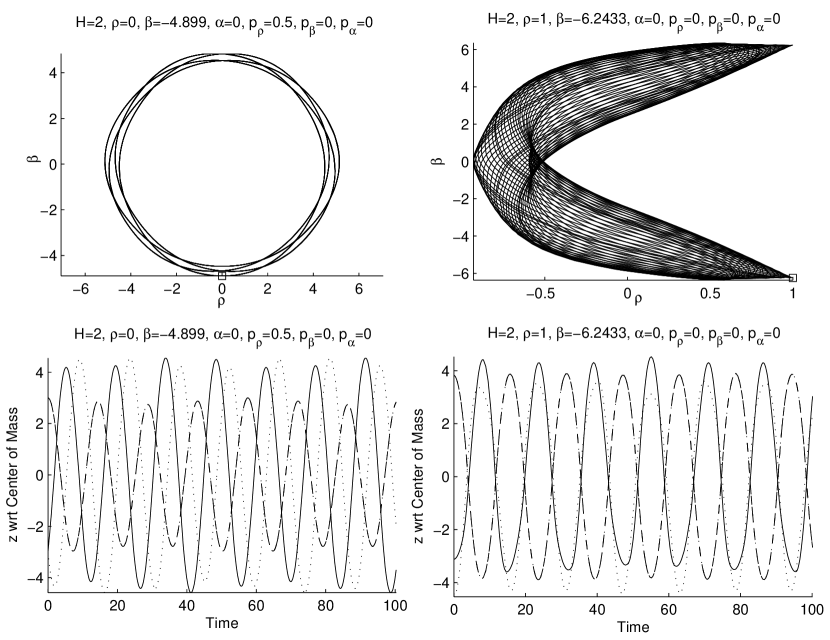
Figure 3: Annulus (on the left) and pretzel (on the right) orbits for 500 time steps and $H=2$.  The initial conditions for the plots on the left are: $\rho=0,$ $\alpha=0,$ $p_{\rho}=0.5,$ $p_{\beta}=0,$ $p_{\alpha}=0$.  $\beta$ will be calculated so that eq. (7) is satisfied initially.  The initial conditions for the plots on the right are: $\rho=1,$ $\alpha=0,$ $p_{\rho}=0,$ $p_{\beta}=0,$ $p_{\alpha}=0$.

Similarly, it is not surprising that we recover the two-body case if we choose two momentum and position coordinates to be zero initially.  For example, if we set $\rho_{0}=0$, $\ \alpha_{0}=0$ and $p_{\rho 0}=0$, $\ p_{\alpha 0}=0$, then the box-particle will move on a line parallel to the $\beta$-axis.  In this case, the $z(t)$ plots show only two distinguishable trajectories, because we have actually two pairs of particles moving.  Unlike the reduction to the three-body case from the equal mass four-body problem, we have here a reduction to an equal mass two-body problem.

3.2 Three-Dimensional Trajectories

Of course the more interesting situation is when there is motion in all spatial directions, generating three-dimensional patterns.  Changing the initial conditions a little bit from those used for the plots shown in Figure 3 by giving, for example, a small momentum along the $\alpha$ direction gives us the three-dimensional trajectories (Figure 4). Not surprisingly, these patterns are direct generalizations of what we observed in Figure 3, since the motion in the $\alpha$ direction simply perturbs the patterns previously obtained in the $\left(\alpha,\beta\right)$ plane when we set $\alpha=0$ and $\ p_{\alpha}=0$, initially.  Essentially the original hex-particle patterns develop a “thickness” in the $\alpha$ direction.

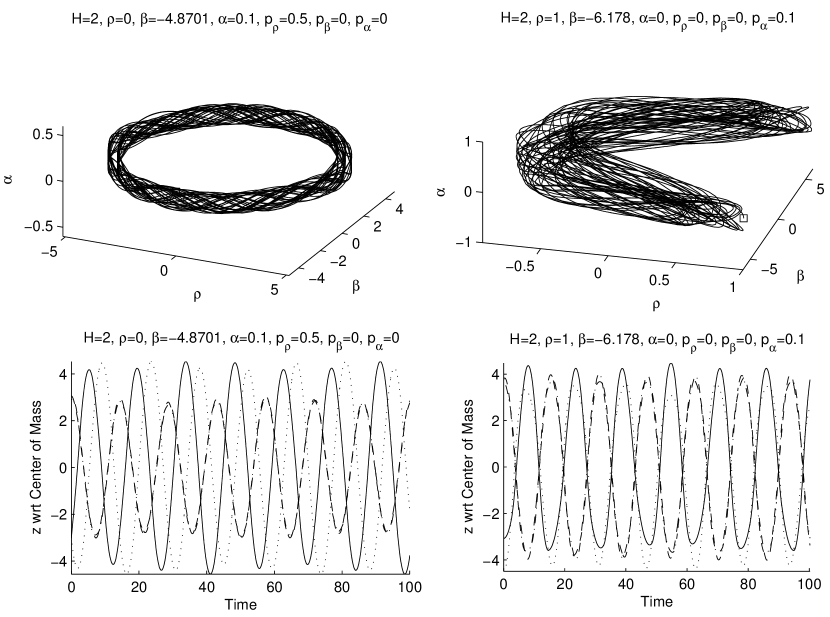
Figure 4: Annulus and pretzel orbits for 500 time steps and $H=2$.  The initial conditions for the plots on the left are: $\rho=0,$ $\alpha=0.1,$ $p_{\rho}=0.5,$ $p_{\beta}=0,$ $p_{\alpha}=0$. The Lyapunov exponent for this trajectory was calculated to be 1.214$\times$$10^{-2}$. The initial conditions for the plots on the right are: $\rho=1,$ $\alpha=0,$ $p_{\rho}=0,$ $p_{\beta}=0,$ $p_{\alpha}=0.1$. The Lyapunov exponent for this trajectory was calculated to be 7.350$\times$$10^{-3}$.

For the three-dimensional annulus, we chose initial conditions to show that a non-zero $\alpha_{0}$ induces a non-zero $p_{\alpha}(t)$, even if $p_{\alpha 0}=0$.  It is also interesting to compare the peaks of Figure 3 with those of Figure 4.  We see that the three-dimensional trajectories experience a small deviation (near the peak) in the trajectories of the two particles that were exactly the same for the two-dimensional box-particle trajectories.  The more we increase the value of the initial conditions $\alpha_{0}$ or $p_{\alpha 0}$ the bigger the deviation, and in the $(\rho,\beta,\alpha)$ space, the particle will have a larger amplitude in the $\alpha$ direction.

To further investigate the trajectories that can be obtained in the full three-dimensional case, we follow the method in [9] - that is using initial condition constraints of fixed-energy (FE) and of fixed-momentum (FM). Since the Hamiltonian is a homogeneous function of the coordinates and momenta, it can always be rescaled to unity by an appropriate rescaling of the phase space variables. Fixed energy conditions are equivalent to rescaling all variables in terms of $\eta$, as noted previously. Anticipating future comparison with the relativistic case, we find it convenient to choose different initial values for $H,\rho,\beta,\alpha,p_{\rho},$ and $p_{\beta}$, adjusting $p_{\alpha}$ using the Hamiltonian constraint (7), and check that $H$ remains at its initial value throughout the motion (Figures 3, 4, 6, 14, 16, 17).  We have chosen to vary $p_{\alpha}$, to more easily facilitate comparison with the previous results in the equal-mass 3-body case [9].  Similarly for the fixed-momenta case (Figure 5, Figure 8 - 13) , we will choose $\rho,\beta,\alpha,p_{\rho},p_{\beta}$ and $p_{\alpha}$ while allowing $H$ to vary as the initial conditions vary. This allows us to more easily select qualitatively different types of motions.

We imposed error tolerances on the Matlab ODE routine and checked that the total energy of the system remained constant throughout the motion for any given set of initial conditions.  Since we were using an improved version of the code, we were able to get the error down to $10^{-8}$ in most cases, and always less than $10^{-7}$.

As noted above, small perturbations of the three-body case yield three-dimensional trajectories that usually have a nice shape similar to that of the three-body case if projected onto one of the planes $(\rho,\beta),(\rho,\alpha)$ or $(\beta,\alpha)$.  However, the third axis is generally just a periodic oscillation with no real pattern relative to the other axes, as in Figure 5.  This trajectory’s motion is characterized by the symbol sequence $\overline{CB^{2}CB^{2}CB^{6}}$. The Lyapunov graph shown in the bottom-middle is the ‘fixed’ Lyapunov graph where the perturbation was sufficiently small to prevent orbital bifurcation. The bottom right figure displays orbital bifurcation where, after some number of collision steps, the trajectories reconverge suddenly. This is seen by the sudden curve downwards. In theory, if this trajectory was run for a sufficiently large number of collision steps, the value would converge to the Lyapunov exponent of the ‘fixed’ trajectory.

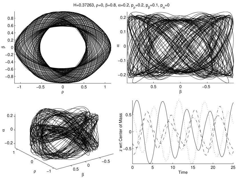
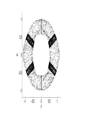
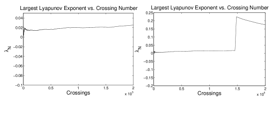
Figure 5: The top two plots show the trajectory from two different directions.  It is clear that while being a nice annulus shape in the $(\rho,\beta)$ plane, the plot is much more random in the $(\beta,\alpha)$ plane, although one can still observe a semi-periodic pattern.  The bottom-left isometric plot of the trajectory shows that the periods of oscillation in the various axes do not line up nicely for these initial conditions.  The bottom-right plot show the four particle positions vs. time; the symbol sequence is $\overline{CB^{2}CB^{2}CB^{6}}$. The bottom-left figure was obtained using the collision to collision mapping solution. Note the same size, shape and banding structure between the two figures. – these are faint in the diagram at the upper left, but are visible. The Lyapunov graph is shown at the bottom-middle with a calculated Lyapunov exponent of 2.138$\times$$10^{-2}$. The Lyapunov graph on the bottom-right is an example of orbital bifurcation where the trajectories reconverge after some number of collision steps. It is also seen that even in the ’fixed’ trajectory, the Lyapunov graph does not clearly converge. This seems likely due to problem within the numerics of the system.

However, cases where these periods do line up can be obtained with carefully chosen initial conditions.  For example, figure 6 shows a trajectory that has a pretzel form when projected onto two of the planes ($(\rho,\beta)$ and $(\rho,\alpha)$), and an annulus when projected onto the third ($(\beta,\alpha)$).  The three-dimensional isometric (in which there is no perspective so that objects further away do not appear smaller) view shows a periodic three-dimensional path - a qualitatively new feature that has no analogue in the 3-body system.  The motion here is described by $\overline{(CB^{2}CB^{2}CB^{6})^{2}CB^{6}}$, which is very similar to the previous figure. This trajectory also displays orbital bifurcation in its Lyapunov graph (shown bottom-right). In this case, the trajectories do not reconverge in the 200,000 collision steps in this simulation.

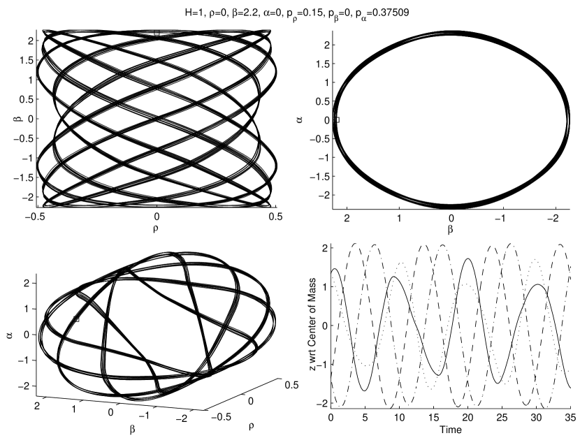
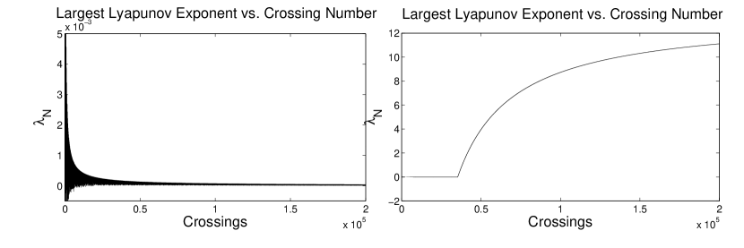
Figure 6: The layout of the plots is the same as Figure 5.  In this case however, we see that from every direction the trajectory forms a recognizable two-dimensional plot (third direction is not shown, but it is a pretzel similar to the top-left).  Since the periods of the motions in various axes are compatible in this case, we see from the isometric plot (middle-left) that a fully three-dimensional periodic trajectory exists.  Note that FE ($H=1$) constraints were used in this case for convenience. At the lower-left is the Lyapunov graph for this trajectory, whose Lyapunov exponent was calculated to be 2$.835\times 10^{-5}$ . The figure at the lower right is another example of orbital bifurcation.

To give an even better idea of the types of paths that can be obtained with compatible periods, another example is shown in Figure 7.  The symbol sequence for this trajectory is similar to the other example in that it contains mostly sets of $CB^{2}$ and $CB^{6}$; however $CB^{12}$ also shows up occasionally.

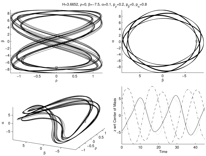
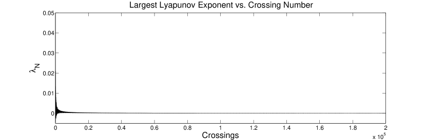
Figure 7: Another example of a periodic three-dimensional path. The Lyapunov graph for this trajectory is at the bottom, and its Lyapunov exponent was calculated to be $3.323\times 10^{-5}.$

Suffice it to say that many interesting trajectories can be obtained, although most are generalizations of the three-body case, as seen in the previous section, or are simply chaotic.  As expected we find that the latter case produces the same type of dense orbits in three-dimensions as its 3-body counterpart did in two.

3.3 Trajectory Plots of Special-Cases

We will now focus our attention on the various special cases that we can attain by starting particles very close to one another.  For example, we can put two sets of two particles together, and we expect those two to repeatedly cross one another, while on average the two pairs behave as a equal-mass two body system.  Similarly we could put three particles very close together and one separate.

From this and the fact that we have equal masses we will consider six initial configurations: 1+1+1+1, 2+2, 3+1, 2+1+1, 1+2+1 and 1+1+2, where “a+b+c” notation indicates the relative size of the initial $z$ values, with largest at the left and smallest at the right; a number larger than unity indicates that the difference between the $z$-values of these particles is small relative to all other spacings. For example, “2+1+1” denotes that we have a pair of particles starting close together (relative to the other spacings) with the greatest $z$ values, and two independent (far apart) particles with the lower two $z$ values.  Strictly speaking the 1+1+2 and 2+1+1 cases are symmetric (equal masses) and indeed they produce similar plots as we will see.

For each of these possible cases, we construct plots of  the box-particle in $(\rho,\beta,\alpha)$ space and the associated plot of particle positions on the line.  The easiest way to find suitable initial conditions is to use (5) to choose $\rho,\beta$ and $\alpha$ so that we get suitable particle starting positions, and set the momenta to zero.  Thus we use the fixed-momenta conditions and allow $H$ to vary.  Only one angle of the $(\rho,\beta,\alpha)$ plots is shown, though the captions describe them in more detail.

Figure 8 shows the case where the four particles begin spaced at equal unit spacing with no momentum.  Predictably they are all drawn together and cross at the same point, continuing this pattern indefinitely.  Since all four particles always ‘collide’ at the same time step, the symbol sequence in terms of $A$, $B$, and $C$ is undefined. Instead the motion reduces to that of a single body of mass $4m.$  The box particle travels back and forth along a line in $(\rho,\beta,\alpha)$ space, with all particles simultaneously crossing at the origin. This motion is unstable: a slight change in any of the initial conditions (either via a small displacement or small momentum) throws the system into chaos, as shown in the bottom two images of Figure 8.

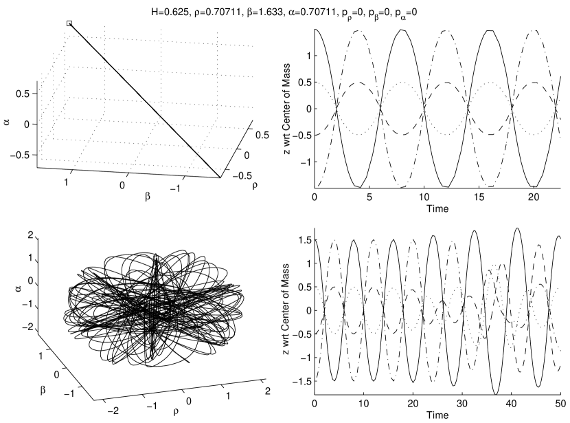
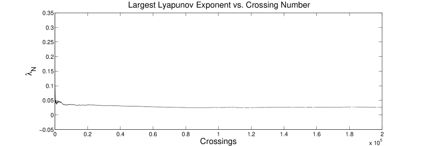
Figure 8: The 1+1+1+1 case.  The $(\rho,\beta,\alpha)$ plot is a single line diagonal through the three axes, as shown here.  The bottom two images show what happens if we change the initial conditions very slightly (here we set $\rho^{\prime}=\rho+0.0001$).  As can be seen on the $(z,t)$ plot, the system quickly degenerates into chaos. The Lyapunov graph for the perturbed trajectory, whose Lyapunov exponent was calculated to be$2.697\times 10^{-2}$ appears at the bottom.

In Figure 9, we see the case with two pairs of particles, denoted as 2+2. Each of the two tightly bound states undergo mildly irregular motion (where each particle randomly attains the maximal separation from the origin), but that the orbit of each bound pair about the other is quite regular, with fairly constant frequency and amplitude.  Numerically we estimate the frequency of the oscillation of the pairs at $0.16$ cycles per time step, with an amplitude of $1.2$.  The motion is a string of $A$’s, $B$’s, and $C$’s without any discernible pattern, the only noticeable feature being that the $B$’s always occur in pairs ($B^{2}$).

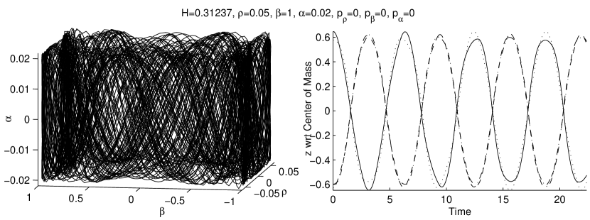
Figure 9: The 2+2 case.  The $(\rho,\beta,\alpha)$ plot is a very dense pretzel if projected onto two of the planes, and an almost fully filled square in the third. The Lyapunov exponent for this trajectory was calculated to be $1.307\times 10^{-2}.$

Figure 10 shows the  3+1 case with three particles closely bound together.  These undergo a mildly chaotic orbit that itself regularly oscillates with an amplitude of about $1.4$ and a frequency of $0.15$ cycles per time step about the 4th particle in a loosely bound state.  The symbol sequence is mostly $B$’s, with $A$ or $C$ occasionally appearing.  Note that while we still do not see any $B^{1\text{'}}$s here, we do see some odd numbered groups of $B$’s.

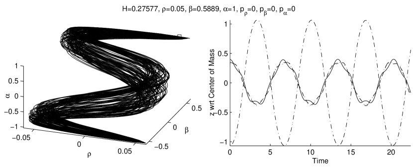
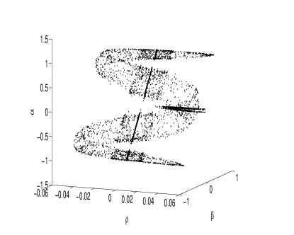
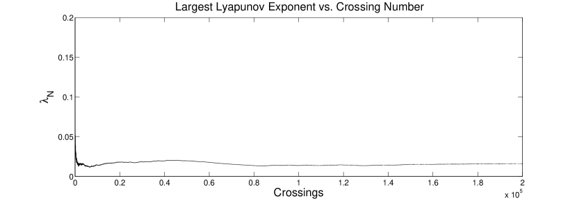
Figure 10: The 3+1 case.  The $(\rho,\beta,\alpha)$ plot is an almost two-dimensional pretzel rotated sideways. The figure below it was obtained using the collision to collision mapping solution. Once again, the dimensions and banding structure are common features of the two plots, though these features are only faintly visible in the upper right graph. The bottom figure is the Lyapunov graph for this trajectory, whose Lyapunov exponent was found to be $1.609\times 10^{-2}.$

Figures 11-13 show the cases where only one pair of particles is closely bound, namely 2+1+1, 1+2+1 and 1+1+2 respectively. Fig. 11 generates a thick ‘fish’ pattern: the tightly bound state of two particles executes a $\overline{B^{4}A}$ motion with respect to the other two.  However the full 4-body sequence does not exhibit any clear pattern.

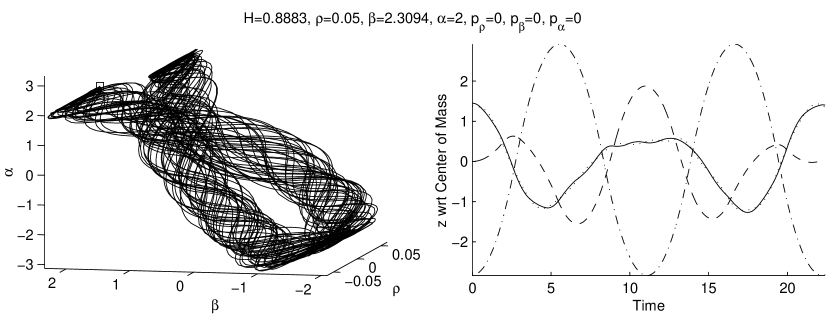
Figure 11: The 2+1+1 case.  The $(\rho,\beta,\alpha)$ plot is a “fish” type shape in one plane, and a mess in the others (as seen in the previous sections). Similar “molecular” structures have been noted previously in the relativistic [9, 10] and non-relativistic [15] 3-body cases. The Lyapunov exponent for this trajectory was calculated to be $2.336\times 10^{-2}.$

Fig. 12 illustrates a similar kind of motion, in which the tightly bound state undergoes a $\overline{B^{10}A}$ motion with respect to the other two; the time period shown on the graph is too short to see this explicitly in the figure.  Again the 4-body crossing sequence has no discernible pattern.

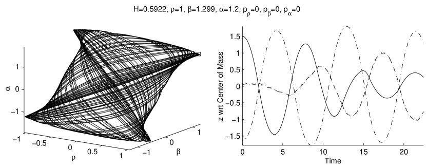
Figure 12: The 1+2+1 case.  The $(\rho,\beta,\alpha)$ plot is an almost two-dimensional pretzel rotated on two axes and skewed on one. The Lyapunov exponent for this trajectory was calculated to be $1.133\times 10^{-2}.$

In Fig. 13 we see another similar trajectory, but with subtly distinct features.  The two particles are not as tightly bound as in the preceding cases, but (over the time scales we observed) execute a highly regular oscillatory interaction with the other two particles.  The four particles repeatedly come very close together before executing near parabolic motion about the centre of mass.  However after about 80 time steps the trajectory degenerates into chaos.  While the paired particles remain bound, they eventually fall out of the parabolic motion and begin to move chaotically with respect to the other particles.  No pattern is obvious in the symbol sequence.

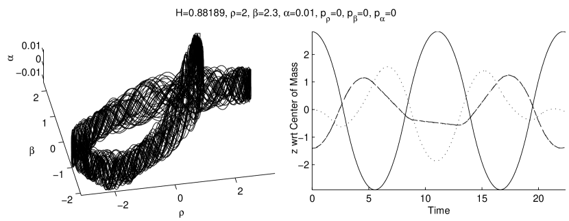
Figure 13: The 1+1+2 case.  The $(\rho,\beta,\alpha)$ plot is a very nice “fish” shape in one plane. The Lyapunov exponent for this trajectory was calculated to be $2.842\times 10^{-2}.$

3.4 Poincare Plots

We will now examine the Poincare plots of these trajectories in the Newtonian system.  Unfortunately, this turns out to be much more difficult in the four-body case than it was in the three-body.  The reason is that in the three-body system, the Poincare plots were a collection of points in two-dimensions [9, 10], while in the four-body system they are a collection of points in three dimensions.  The latter collection is much more difficult to visualize since it is impossible for the human eye to determine the depth of a single point on these three-dimensional plots with sufficient precision.  Furthermore, the outer layers of points tend to obscure inner ones exists.  Thus we will examine the Poincare plots of several independent three-dimensional trajectories, and then look at ways of visualizing the “total” Poincare plot, with a broad range of initial conditions combined.

Poincare plots are plots of sections of phase space, affording a comparison of classes of trajectories over a broad range of initial conditions. We shall set $H=1$ throughout. In the equal mass case all of the bisectors of the 3-simplex represent equivalent crossings of particles.  Thus we can plot the crossing of any two particles (equivalent to the $(\rho,\beta,\alpha)$ particle crossing one of the bisectors in the three-dimensional potential) all on the same graph.

In the three-body case the Poincare plot was that of the radial momentum of the simplex particle plotted against its angular momentum every time the particle crossed a simplex bisector [3, 9, 10]. The most natural extension of the construction of these plots to three dimensions is to use spherical coordinates, and plot the radial momentum, denoted here as $p_{R},$ against the two angular momenta squared: $p_{\phi}^{2}$ and $p_{\theta}^{2}$.  More concisely, we define $R$ to be the distance from the origin to our point of crossing in $(\rho,\beta,\alpha)$ space, $\phi$ to be the azimuthal angle in the $(\rho,\beta)$ plane (with $0\leq\phi\leq 2\pi$), and $\theta$ to be the polar angle from the $\alpha$ axis (with $0\leq\theta\leq\pi$).  From this, we denote the associated momenta of $R,\phi$ and $\theta$ as $p_{R},p_{\phi}$ and $p_{\theta}$ respectively.

Specifically, from simple geometry relating our spherical coordinates $(R,\phi,\theta)$ to our Cartesian coordinates $(\rho,\beta,\alpha)$, we have that

$$\sin\phi = \frac{\beta}{\sqrt{\rho^{2}+\beta^{2}}},\quad\quad\quad\;\cos\phi=\frac{\rho}{\sqrt{\rho^{2}+\beta^{2}}}$$ (23)

$$\sin\theta = \frac{\sqrt{\rho^{2}+\beta^{2}}}{\sqrt{\rho^{2}+\beta^{2}+\alpha^{2}}},\quad\cos\theta=\frac{\alpha}{\sqrt{\rho^{2}+\beta^{2}+\alpha^{2}}}$$

and the unit vectors for these spherical coordinates are:

$$\hat{R}=\left[\begin{array}[]{c}\cos\phi\sin\theta\\ \sin\phi\sin\theta\\ \cos\theta\end{array}\right],\quad\hat{\phi}=\left[\begin{array}[]{c}-\sin\phi\\ \cos\phi\\ 0\end{array}\right],\quad\hat{\theta}=\left[\begin{array}[]{c}\cos\phi\cos\theta\\ \sin\phi\cos\theta\\ -\sin\theta\end{array}\right]$$ (24)

The desired momenta are:

$$p_{R}=\hat{R}\cdot\vec{p},\qquad p_{\phi}=\hat{\phi}\cdot\vec{p},\qquad p_{\theta}=\hat{\theta}\cdot\vec{p}$$ (25)

where $\vec{p}\equiv(p_{\rho},p_{\beta},p_{\alpha})$ is the momentum vector in $(\rho,\beta,\alpha)$ space.  Then by substituting (23) and (24) into (25), we can find an expression for the momenta in terms of $\rho,\beta,\alpha,p_{\rho},p_{\beta}$ and $p_{\alpha}$:

$$p_{R} = \frac{p_{\rho}\rho+p_{\beta}\beta+p_{\alpha}\alpha}{\sqrt{\rho^{2}+\beta^{2}+\alpha^{2}}}$$

$$p_{\phi} = \frac{-p_{\rho}\beta+p_{\beta}\rho}{\sqrt{\rho^{2}+\beta^{2}}}$$ (26)

$$p_{\theta} = \frac{p_{\rho}\rho\alpha+p_{\beta}\beta\alpha-p_{\alpha}(\rho^{2}+\beta^{2})}{\sqrt{(\rho^{2}+\beta^{2}+\alpha^{2})(\rho^{2}+\beta^{2})}}$$

Thus we can use (26) to plot $p_{R}$ , $p_{\phi}^{2}$ and $p_{\theta}^{2}$ whenever two of the four particles cross one another.

3.4.1 Single Trajectory Poincare Plots

As we will discover further on, it becomes very difficult to visualize a complete Poincare plot in three dimensions. We therefore will build up to this case by first examining individual Poincare plots generated from single trajectories. Note that all of the following Poincare plots were produced using both methods and found to be exactly the same, checking the validity of the following results.

To keep things simple, we will first look at the case where our trajectory is in two dimensions.  This should result in a two dimensional Poincare plot as well, as in the three-body case.  Since $p_{\alpha}$ is varied to keep the initial conditions consistent, we will arbitrarily choose $\beta$ and $p_{\beta}$ as the variables that we set to zero, thus making it into a two dimensional trajectory as seen in previous sections.

Our intuition is indeed correct, as can be seen in Figure 14.  There a two-dimensional pretzel shape produces a two-dimensional Poincare plot that coincides with those seen in the three-body case, consistent with the quasiperiodic motion of this trajectory. As expected, the value of the $p_{\phi}$ (the momenta of the azimuthal angle) remains zero throughout.  This can also be seen from (26), with $\beta=0$ and $p_{\beta}=0$. More importantly, this confirms that the Poincare plots of the four-body system will be generalizations of the three-body system, as was seen with the trajectories, validating our approach for generating these plots.

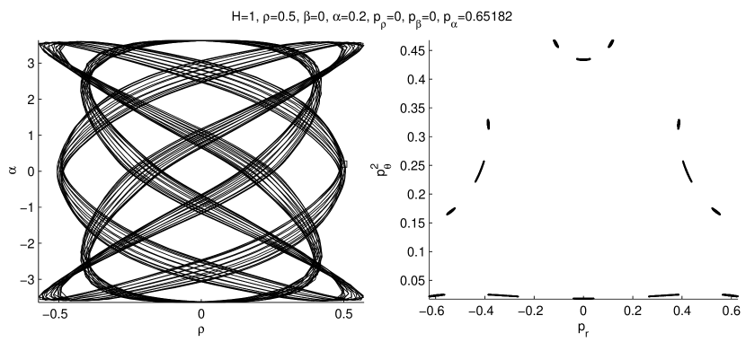
Figure 14: The trajectory and Poincare plots for a two-dimensional pretzel.  Note that the trajectory is shown for five hundred time steps, while the Poincare section is generated from five thousand time steps.  The latter is required to generate enough points from a single trajectory to show a meaningful plot.

Now, we will look at the Poincare plots for some of the “nicer” three-dimensional trajectories.  From Figure 6 we generate a Poincare plot that is given in figure 15, shown from a few angles.

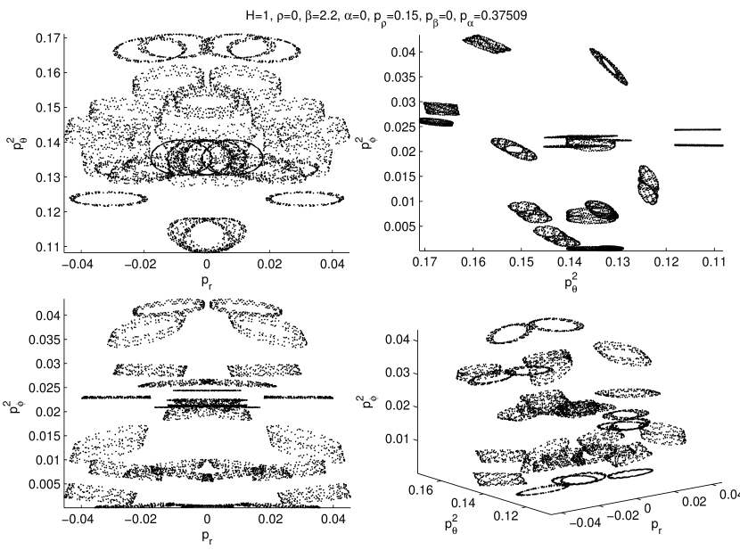
Figure 15: The Poincare plot of the trajectory in Figure 6, shown here from all three directions, and from an isometric perspective.  The broad circular bands are indicative of the quasiperiodic character of this trajectory.

This plot is extremely interesting in that it does not seem to exhibit the same patterns as the three-body case.  Remembering that this shape is actually a combination of annuli and pretzels, we can begin to see some patterns.  First, the elliptical shells (they are actually extruded ellipses) in this plot are very similar to the ellipses in the pretzel section of the three-body Poincare plots, although no geometric pattern is immediately obvious.  Second, if we compare the scale on this plot to that of the previous and final Poincare plots (see next section), we discover that indeed it is only occurring in a smaller region of the larger plot - potentially the three-dimensional equivalent of the “pretzel region” seen in the three-body case (albeit more complex, since this trajectory is not exclusively a pretzel).

Another example is shown in Figure 16.  We can see here that because of the skew of the shape in the trajectory plot, the Poincare plot is not nearly as structured as the previous ones.  Still, we can note some pattern, although it is much more difficult to see in three dimensions. Each trajectory is quasiperiodic, but spread over a three dimensional space, with the pretzel trajectories forming a non-overlapping knotted structure. As with the 3-body case, the Poincare plots consist of circles with some width. These occupy a three dimensional volume, and the more loosely dispersed dots form a “shell” over the top of the Poincare plot.

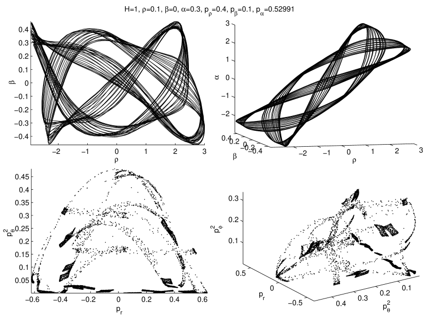
Figure 16: The top two images show the trajectory plot, while the bottom two show the corresponding Poincare plot.  Although it is difficult to see on static images, the more loosely dispersed dots form a sort of “shell” over the top of the Poincare plot.  We can already see the trouble with visualizing this, even with only a single trajectory shown! The Lyapunov exponent for this trajectory was calculated to be $4.700\times 10^{-4}.$

Examining other Poincare plots of three-dimensional trajectories, we reach the limits of this particular approach.  As we saw earlier, very few initial conditions actually produce nice three-dimensional paths, and the ones that do not produce similarly uninformative Poincare plots.  It is possible that if run for a significant number of time steps these plots would materialize into more than just a random collection of points in space, but the amount of computation required to produce the hundreds of thousands of time steps that would be required to check this is daunting, and probably not the best use of resources.  Moreover, it becomes increasingly difficult to visualize these plots as the number of time steps increases.

However, there is some support for the conjecture that more time steps will reveal better patterns.  More time steps yield more particle crossings, and thus more points on the Poincare plot.  Instead of extending the length of the trajectory though, we can instead choose initial conditions such that two particles are extremely close together and cross frequently.

We illustrate this with an example in figure 17.  The motion of the box-particle is characterized by a huge number of $A$’s with an occasional $B$ and $C$ (as we would expect due to the large number of collisions between the two tightly bound particles).  This trajectory produces a very nice three dimensional shape, demonstrating  that three-dimensional Poincare plots can be considerably more complicated than their two-dimensional counterparts.

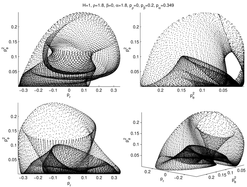
Figure 17: The Poincare plot of a highly refined trajectory.  The box-particle trajectory is uninteresting: it is basically just a two-dimensional annulus rotated approximately forty-five degrees in two axes.  Notice the complex patterns displayed even in the Poincare plot for a single trajectory! The Lyapunov exponent for this trajectory was calculated to be $2.602\times 10^{-3}.$

To conclude this section, we plot a graph (figure 18) that contains all of the previous Poincare plots combined, just to give an idea of scale.

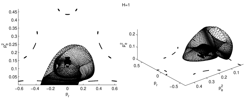
Figure 18: The top and isometric views of the combined Poincare plots in this section.  Note the relative scale.

3.4.2 3D Poincare plots

Now we move on to the problem of visualizing the complete Poincare plot, with a variety of initial conditions included.  The traditional approach generally involves choosing a range of initial conditions that fill in the important regions, and plotting all of the points on a combined two-dimensional plot.  This approach has two immediate problems in three dimensions.

First, the amount of space to fill in three - as opposed to two - dimensions makes the task of manually choosing initial conditions formidable.  There is no reasonable way of ensuring that all of the possibilities have been covered, especially since there are a large number of variations and combinations of three-dimensional trajectories.  We attempted to address this problem by automating the generation of data over a specific range of initial conditions. With five independent variables the number of possible plots is very large, necessitating a significant reduction in the number of time steps for each initial condition.  We generated Poincare data for each trajectory for five hundred time steps, giving about 1,000 Poincare points per trajectory. The second problem is that of effectively visualizing all of these discrete points in three-dimensional space. We approached this problem by converting the data into volumetric density data, separating out the space into millions of tiny three-dimensional boxes, assigning a position corresponding to the location of the box and a value corresponding to the number of Poincare points that fall inside.  This yields a large three-dimensional grid of values, each representing the density of points in the Poincare plot at that approximate location.

The advantage of this approach is that we can now easily take slices and contours, colouring them according to the volumetric value at the corresponding locations. This effectively decomposes the three dimensional data into a series of two dimensional plots. However there are disadvantages, the most significant being that we are more limited in our ability to zoom in to see self-similar patterns and structures at the resolution the number of chosen grid points.  Although we can always use more grid points, we quickly arrive at a situation in which there are too few points in a small region to satisfactorily “fill up” the density data. However we expect that some of the other important features, like the highly saturated regions of chaos, will show up well in our new plots.  Since those regions have a large number of points, they should get a very high density value and thus stand out from the surrounding region.  With enough points and a small enough grid, it should also still be possible to see the general shape of the Poincare plot in three dimensions.

We will first examine two special slices: that of $p_{\phi}=0$ (the “bottom” slice) and $p_{\theta}=0$ (the “side” slice).

For the bottom slice, we can use the condition $p_{\phi}=0$ to select the applicable points. This yields 400,000 points out of the 12 million that we generated.  As we see in Figure 19, this two-dimensional slice compares quite well to the 3-body case [9].  The figure suggests the presence of mixed regions of chaos and integrability, as further implied by figures 20 and 21.

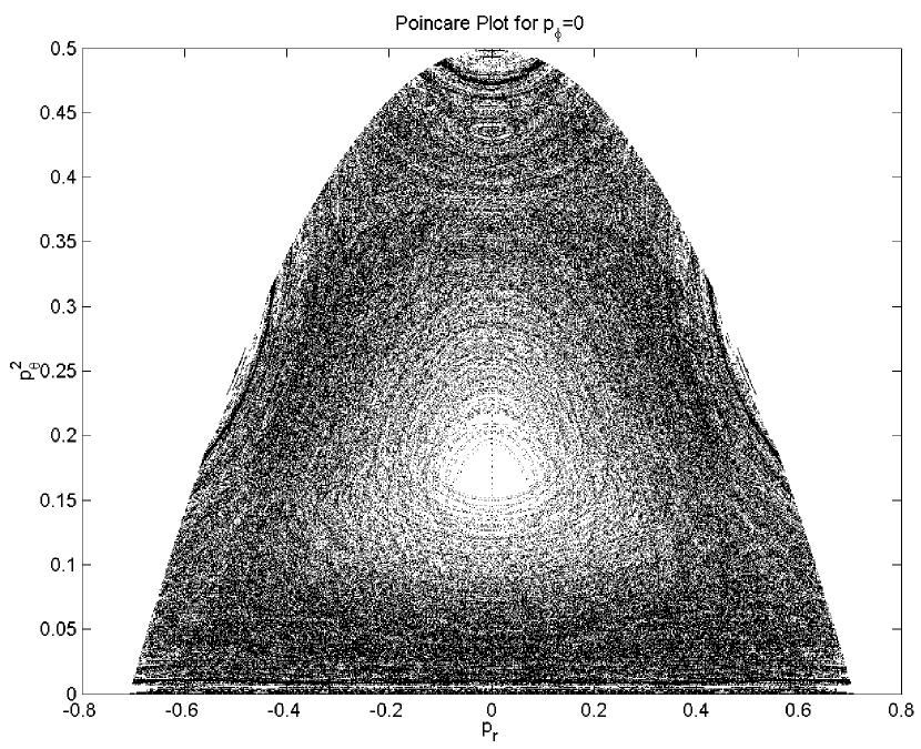
Figure 19: The bottom slice of the complete Poincare plot (~400,000 points).

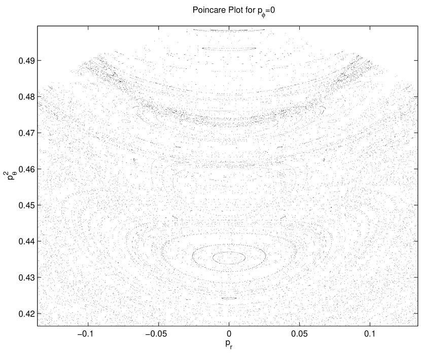
Figure 20: A zoomed-in image of the top portion of Figure 19.  Notice the complex fractal-like patterns that show up as we zoom closer.

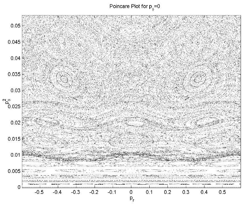
Figure 21: A zoomed-in image of the bottom portion of Figure 19.

For the side slice, we could not use the condition of $p_{\theta}$ being exactly zero.  $p_{\phi}=0$ will be true for any of the two-dimensional trajectories in planes passing through the $\alpha$ axis.  Since $p_{\alpha}$ is calculated from $H=1$, most - if not all - of the two-dimensional trajectories in our parameter scan will be on planes passing through the $\alpha$ axis (initial conditions with $p_{\alpha}=0$ are extremely unlikely).  However, $p_{\theta}=0$ would only be true of a trajectory that remained in a cone rooted at the origin.  Hence we use the constraint of $p_{\theta}$ being “close” to zero, instead of exactly zero to get an equivalent slice. We used $p_{\theta}^{2}<0.0005$ which produced about five-hundred thousand points.

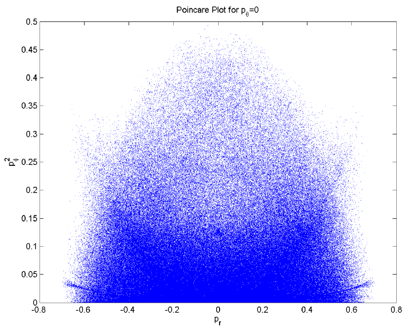
Figure 22: The side slice of the complete Poincare plot (~500,000 points).  Note that this plot does not display the fractal-like properties of the bottom slice (Figure 19).

The first thing that we notice is that the side slice does not display the same patterns and fractal-like properties as the bottom slice.  This could be due either to too few time steps or to a failure to cover a sufficient range of initial conditions.  It could also possibly mean that spherical coordinates are not the best choice for a generalization of Poincare plots; perhaps cylindrical coordinates or another transformation would have produced more revealing results.  However it is also possible that the system simply does not demonstrate any clearly definably pattern when sliced along the $p_{\theta}=0$ plane.

We can get an idea of the true three-dimensional shape of this Poincare graph by slicing the volume into multiple $p_{R}=k$ planes, each coloured according to density with brighter colours being higher densities.  Unfortunately this approach allows us to see little more than the general “shape” of the plot.  As the diagrammatic slices are not enlightening we shall not present them here.

4 Lyapunov Exponents

To compute Lyapunov exponents for the 4-body system,  we employ a method due to Benettin et.al.[16] for calculating the largest Lyapunov exponent, using number of collisions instead of time elapsed for calculating the largest Lyapunov exponents. First, we take an initial deviation $\delta(0)$ away from a reference trajectory that has already been calculated for $m$ collisions (the total number of collisions). This perturbed trajectory is then calculated for $j$ collisions. Note that $m$ denotes the number of collision steps (with $k$ denoting the step number) and $j$ is an integer that denotes the sampling rate. For example, if we consider 100,000 collisions sampled every 10th collision, then $m=100,000$, $j=10$, and $k$ would vary from 1 to 10,000. We assume that $m/j$ is an integer.

We then compare the reference and perturbed trajectory after $j$ collisions (or after one step number) and calculate $\delta^{\prime}(1)$, the difference between our reference and perturbed trajectory. We rescale this to have the same magnitude as $\delta(0)$, and then repeat the process with $\delta(1)$ as the peturbation. At the $k$ th step we obtain the deviation $\delta^{\prime}(k)$, and rescale it to have the same magnitude as $\delta(0)$, which then becomes the new initial deviation $\delta(k)$, calculated generally as shown in the expression

$$\delta\left(k\right)=\frac{\delta^{\prime}\left(k\right)}{d_{k}}\left\|\delta\left(0\right)\right\|\text{ \ \ \ \ where \ \ \ \ \ \ }d_{k}=\left\|\delta\left(k\right)\right\|$$

where $\delta^{\prime}\left(k\right)$ is computed relative to the original trajectory from $k=(n-1)$ to $k=n$ ($n=1,2,...,m/j$). This process terminates for $k=m/j$. The largest Lyapunov exponent ($\lambda_{1}$ in our notation) is then obtained from

$$\lambda_{1}=\lim_{n\rightarrow\infty}\left[\frac{1}{nj}\sum_{k=0}^{n}\ln\left(d_{k}\right)\right]$$ (27)

Below is a table of calculated values for Lyapunov exponents for figures shown throughout the paper. All of the values below are considered accurate to $10^{-5}$, where all quantities in the table should be multiplied by $10^{-4}$. The uncertainty arises from the small fluctuations in the Lyapunov exponent graph which are on the order of $10^{-5}$ for all graphs. Values for Lyapunov exponents for bifurcated trajectories are not included because the graphs and trajectories do not converge and do not exhibit Lyapunov-like behavior and therefore the exponents are not relevant. Only 3 dimensional trajectories are considered below so they are readily comparable to one another. We have not computed Lyapunov exponents for the effective unequal-mass 2 dimensional (3-body) motions in figures from Figure 3 (in which one coordinate and its conjugate momentum are fixed to always be zero) since we are concerned here only with equal-mass 4-body case. A study of the Lyapunov exponents for the unequal-mass 3-body case remains an interesting subject for investigation.

Table of $\lambda_{1}$Values (after 200,000 collisions) $\times$ $10^{-4}$
Fig. 4 “Thick”Annulus	121.4	Fig. $8{}^{\text{\textdagger}}$  1+1+1+1	269.7	Fig. 13 1+1+2	284.2
Fig. 4 “Thick” Pretzel	73.50	Fig. 9   2+2	130.7	Fig. 16 Poincare Pretzel	4.700
Fig. $5$ Chaotic Annulus	213.8	Fig. 10   3+1	160.9	Fig. 17 Poincare Annulus	26.02
Fig. 6 Dense Pretzel	.2835	Fig. 11   2+1+1	233.6	Chaotic Trajectory*	395.5
Fig. 7 3D Periodic Trajectory	.3325	Fig. 12   1+2+1	113.3

†The value of the Lyapunov exponent is for the perturbed plot in the bottom left.

*initial conditions $\rho=0.1000$, $\beta=0.5000$, $\ \alpha=-0.2000$, $\ p_{\rho}=0.2000$, $p_{\beta}=-0.2000$ and $\ p_{\alpha}=-0.3000$.

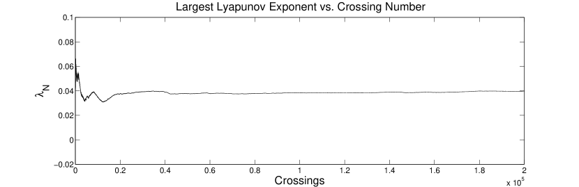
Figure 23: A plot of the largest Lyapunov exponent for the Chaotic Trajectory. This trajectory was considered as a random set of initial conditions that produced a chaotic trajectory in order to give a numerical reference point against which we could compare other Lyapunov exponents.

Looking at the Lyapunov exponents, a trend of values emerge. First, trajectories that were considered to be mostly chaotic in nature (based on the Lissajous figures accompanying them) have Lyapunov exponents on the order of $10^{-2}.$ For trajectories that are periodic, the Lyapunov exponents are on the order of $10^{-5}.$ For these small Lyapunov exponents, the exact numerical values for the exponents are more uncertain because the small fluctuations in these graphs are on the order of the Lyapunov exponent. The mean value of the graphs over the last hundred collisions are used to obtain a numerical estimate. There also seems to be a range of intermediate values for Lyapunov exponents for quasiperiodic trajectories in the range of $10^{-3}$to $10^{-4}.$

One noteworthy feature of some Lyapunov graphs is orbital bifurcation, in which the apparent stabilization of the largest Lyapunov exponent is punctuated by a sudden increase toward a new value. We found this to occur in a small number of graphs we analyzed (particularly figures 5 and 6 as shown). Further inspection of this phenomenon indicated that the sudden increase was caused by differing collision order between the unperturbed and perturbed trajectories, causing the positions of the particles at a given collision number to differ substantively.

The cause of this difference in collision order was because the perturbed trajectory underwent an extra collision that the unperturbed trajectory did not. Specifically in both cases, the unperturbed trajectory approached a near 2-2 collision (where a left and right pair of particles are about to collide). In the unperturbed case, pair one crossed then pair two, whereas for the perturbed case pair two crossed then pair one. Hence after the first collision the unperturbed system is about to undergo a collision in pair two. Resetting the perturbed trajectory after the first collision will then set it on a course to have pair two collide, even though it has already undergone a pair-two collision. Hence the perturbed trajectory undergoes pair-two collision twice in a row without having had a pair-one collision, putting it one collision behind the unperturbed trajectory. After this the two systems undergo very similar motion, only with a relative switch of two and one collision behind. This switch, along with the lagging of the perturbed system, results in significant differences between the two cases upon comparing the two systems. These differences cause massive divergences in the Lyapunov exponents, seen as discontinuities in the graphs.

Another unexpected phenomena within orbital bifurcation is that in some cases, the bifurcated trajectories reconverged to one another (as seen for figure 5). However, this is not always seen on the time scale that was used for the analysis (as in figure 6).

In order to resolve this, the initial perturbation size was decreased (from $10^{-6}$ to$10^{-10}$ in both cases) so that this phenomenon disappeared and smooth Lyapunov graphs were obtained. By reducing the perturbation size, the two trajectories stay close enough to one another so the switch and extra collision do not occur. However in both cases, each pair of particles are extremely close to each other in the pair, suggesting that what should have occurred is a simultaneous 2-2 crossing instead of the ‘C’ motion of the particles as is seen. Thus, this phenomena may simply be the fault of the numerics and the sensitivity therein.

5 Conclusion

We have carried out the first investigation of the non-relativistic 4-body problem for a one-dimensional self-gravitating system in the equal mass case.  This system is the largest value of $N$ in which the motion can be directly visualized in terms of the motion of a single particle, referred to as the box particle, which is inside a linear potential whose equipotential surfaces are a simplex that has the shape of six square pyramids with their bottoms joined in the shape of a cube. We showed how to classify the motions of this system in terms of braid group operators, and were able to generalize this classification to arbitrary values of $N$.

We find that the trajectories of the box-particle form natural generalizations of the 3-body case, thickening in one direction for small departures from planar motion, in which the box-particle’s position and momentum coordinates are initially zero. A common (and somewhat unexpected) feature is that quasi-periodic motion can appear in certain two-dimensional projections of the box-particle’s trajectory whilst other projections yield an apparently chaotic motion.

We generalized the Poincare plots of these trajectories to be three-dimensional, where the radial momentum of the box-particle is plotted against the two components of its angular momenta in spherical coordinates whenever the box particle crosses a bisector of the equipotential simplex.  While plots for specific trajectories can be straightforwardly constructed, a 3-dimensional Poincare plot over a large variety of initial conditions proves extremely difficult to visualize in any practical sense.  We found that slices for constant azimuthal momenta yielded a fractal pattern, but slices of constant polar momenta yielded no discernible pattern.

Finally, we computed the Lyapunov exponents using the methods of ref. [6] for various trajectories and computed the largest Lyapunov exponents. In general the Lyapunov exponent graphs are quite stable and asymptote to values that seem to correspond to their degree of stochasticity. These numeric results seem quite reliable. Although, in future research analyzing Lyapunov exponents using the collision method, it is important that perturbations are kept sufficiently small to ensure no orbital bifurcation occurs.

Acknowledgments

This work was supported in part by the Natural Sciences and Engineering Research Council of Canada. We are grateful to J. Emerson for helpful discussions.  We are grateful to Steve Blanchet for his contributions to the early development of this work. We are also grateful to Marius Oltean for his technical assistance while working on numerics.

References

- [1] See B.N. Miller and P. Youngkins Phys. Rev. Lett. 81 4794 (1998); K.R. Yawn and B.N. Miller, Phys. Rev. Lett. 79 3561 (1997) and references therein.
- [2] See G. Rybicki, Astrophys. Space. Sci 14 (1971) 56 and references therein.
- [3] H.E. Lehtihet and B.N. Miller, Physica 21D, 93 (1987).
- [4] R.B. Mann and P. Chak, Phys. Rev. E65 (2002) 026128.
- [5] H. Koyama and T. Kinoshi, Physics Letters A295 (2002) 109.
- [6] N.D. Whelan, D. Goodings and J.K. Cannnizzo, Phys. Rev. A42 (1990) 742.
- [7] D. Bukta, G. Karl and B. Nickel, Can J. Phys 78 (2000) 449.
- [8] F.J. Burnell, R.B. Mann and T. Ohta, Phys. Rev. Lett. 90 (2003) 134101.
- [9] F. Burnell, J.J. Malecki, R.B. Mann and T. Ohta, Phys. Rev. E69 (2004) 016214
- [10] J.J. Malecki and R.B. Mann Phys. Rev. E69 (2004) 066208
- [11] C. Reidel and B.N. Miller, Phys. Rev. E 48, 4250–4256 (1993)
- [12] Eric W. Weisstein. “Braid Group.” From MathWorld–A Wolfram Web Resource. http://mathworld.wolfram.com/BraidGroup.html.
- [13] Eric W. Weisstein. “Braid Word.” From MathWorld–A Wolfram Web Resource. http://mathworld.wolfram.com/BraidWord.html.
- [14] Eric W. Weisstein. “Finite Difference.” From MathWorld–A Wolfram Web Resource. http://mathworld.wolfram.com/FiniteDifference.html.
- [15] .L. Rouet, R. Dufour, M.R. Feix 1994, The One-Dimensional Three Body Problem; published in Numerical Simulation and Ergodic Concepts in Stellar Dynamics, (Springer Verlag, Berlin, 1994)
- [16] G. Benettin, L. Galgani and J.M. Strelcyn, Phys. Rev. A14 (1976) 2338.