The gravity dual of supersymmetric gauge theories

on a two-parameter deformed three-sphere

Dario Martelli and Achilleas Passias

Department of Mathematics, King’s College London,
The Strand, London WC2R 2LS, United Kingdom

We present rigid supersymmetric backgrounds for three-dimensional ${\cal N}=2$ supersymmetric gauge theories, comprising a two-parameter $U(1)\times U(1)$-invariant deformed three-sphere, and their gravity duals. These are described by supersymmetric solutions of four-dimensional ${\cal N}=2$ gauged supergravity with a self-dual metric on the ball and different instantons for the graviphoton field. We find two types of solutions, distinguished by their holographic free energies. In one type the holographic free energy is constant, whereas in another type it depends in a simple way on the parameters and is generically complex. This leads to a conjecture for the localized partition function of a class of ${\cal N}=2$ supersymmetric gauge theories on these backgrounds.

1 Introduction and summary

Localization techniques allow one to perform exact non-perturbative computations in supersymmetric field theories defined on a curved Euclidean manifold, thus motivating the systematic study of rigid supersymmetry in curved space. In three dimensions the conditions for unbroken supersymmetry for ${\cal N}=2$ supersymmetric field theories in Euclidean signature have been studied in [1, 2] following the approach of [3]. In these references it was shown that a supersymmetric Lagrangian can be constructed if there exists a spinor $\chi$ or $\tilde{\chi}$ obeying one of the following equations

$$\begin{split}\nabla^{(3)}_{\alpha}\chi-\mathrm{i}(A^{(3)}_{\alpha}+V^{(3)}_{\alpha})\chi+\tfrac{1}{2}H\gamma_{\alpha}\chi+\epsilon_{\alpha\beta\rho}V^{(3)}{}^{\beta}\gamma^{\rho}\chi&=0~{},\\[5.69054pt] \nabla^{(3)}_{\alpha}\tilde{\chi}+\mathrm{i}(A^{(3)}_{\alpha}+V^{(3)}_{\alpha})\tilde{\chi}+\tfrac{1}{2}H\gamma_{\alpha}\tilde{\chi}-\epsilon_{\alpha\beta\rho}V^{(3)}{}^{\beta}\gamma^{\rho}\tilde{\chi}&=0~{},\end{split}$$ (1.1)

arising from the rigid limit [3] of three-dimensional new minimal [4] supergravity. The background fields consist of a metric $g_{\alpha\beta}$, an Abelian gauge field $A^{(3)}_{\alpha}$ coupling to the $U(1)_{R}$ current, a second vector field $V^{(3)}_{\alpha}$ obeying $\nabla^{\alpha}V^{(3)}_{\alpha}=0$, and a scalar field $H$ [1, 2]. In Euclidean signature all fields are in principle complex, except for the metric which is usually required to be real. Furthermore, in general the spinor $\tilde{\chi}$ is not the charge conjugate of $\chi$ [3].

Examples of geometries obeying equations (1.1) were constructed in [5] and [6], before the systematic analysis of [1, 2]. In particular, a $U(1)\times U(1)$-symmetric background, comprising a one-parameter squashed three-sphere, was presented in [5]. The metric may be written as

$$\mathrm{d}s^{2}_{3} = f^{2}(\vartheta)\mathrm{d}\vartheta^{2}+\cos^{2}\vartheta\mathrm{d}\varphi_{1}^{2}+\frac{1}{b^{4}}\sin^{2}\vartheta\mathrm{d}\varphi_{2}^{2}~{},$$ (1.2)

where $\vartheta\in[0,\tfrac{\pi}{2}]$, $\varphi_{1},\varphi_{2}\in[0,2\pi]$, $b>0$ is a constant squashing parameter, and $f^{-2}(\vartheta)=\sin^{2}\vartheta+b^{4}\cos^{2}\vartheta$. The other background fields are summarised in Table 1.

Background fields	$H$	$A^{(3)}$	$V^{(3)}$
Ellipsoid [5]	$\displaystyle-\frac{\mathrm{i}}{f(\vartheta)}$	$\displaystyle\frac{1}{2f(\vartheta)}\left(\mathrm{d}\varphi_{1}-\frac{1}{b^{2}}\mathrm{d}\varphi_{2}\right)$	$\displaystyle 0$

Table 1: The $U(1)\times U(1)$-symmetric background.

Two different $SU(2)\times U(1)$-symmetric backgrounds, comprising a biaxially squashed three-sphere, were presented in [5] and [6], respectively. In both cases the metric may be written as

$$\mathrm{d}s^{2}_{3} = \mathrm{d}\theta^{2}+\sin^{2}\theta\mathrm{d}\phi^{2}+\frac{1}{v^{2}}(\mathrm{d}\psi+\cos\theta\mathrm{d}\phi)^{2}~{},$$ (1.3)

where $\theta,\phi,\psi$ are standard Euler angles on $S^{3}$, so that $\theta\in[0,\pi]$, $\phi\in[0,2\pi]$, $\psi\in[0,4\pi]$ and $v>0$ is a constant squashing parameter. The rest of the background fields in the two cases are summarised in Table 2, where $\sigma_{3}=\mathrm{d}\psi+\cos\theta\mathrm{d}\phi$.

Background fields	$H$	$A^{(3)}$	$V^{(3)}$
$\displaystyle\frac{1}{4}$ BPS [5]	$\displaystyle-\frac{\mathrm{i}}{2v}$	$\displaystyle\frac{1}{2v^{2}}(v^{2}-1)\sigma_{3}$	$\displaystyle\frac{1}{2v^{2}}\sigma_{3}$
$\displaystyle\frac{1}{2}$ BPS [6]	$\displaystyle-\frac{\mathrm{i}}{2v}$	$\displaystyle-\frac{1}{2v^{2}}\sqrt{1-v^{2}}\,\sigma_{3}$	$\displaystyle\frac{1}{2v^{2}}\sqrt{1-v^{2}}\,\sigma_{3}$

Table 2: The two $SU(2)\times U(1)$-symmetric backgrounds.

In all cases the partition function of an ${\cal N}=2$ supersymmetric gauge theory defined on these backgrounds can be computed exactly using localization, and reduces to a matrix model involving the double sine function $s_{\beta}(z)$, where $\beta$ is identified with the parameter $b$ or related to the parameter $v$, respectively.

If a supersymmetric field theory defined on (conformally) flat space admits an AdS dual, it is natural to ask whether a gravity dual still exists, when the field theory is placed on a non-trivial curved background. Gravity solutions dual to gauge theories defined on the backgrounds discussed above were constructed in [7], [8], and [9], respectively. These are described by one-parameter supersymmetric solutions of four-dimensional ${\cal N}=2$ gauged supergravity comprising a self-dual Einstein metric and an instanton for the graviphoton field. In particular, the metrics in these references were Euclidean versions of AdS₄ and Taub-NUT-AdS₄, which can be thought of as metrics on the ball. The holographic free energies of these solutions were shown to agree with the leading large $N$ free energy of the field theory, defined as minus the logarithm of the localized partition function.

In this paper we discuss a family of rigid supersymmetric backgrounds on the three-sphere depending on two parameters, together with its gravity dual. Namely, an asymptotically locally Euclidean AdS metric, whose conformal structure at infinity reproduces the fields $g_{\alpha\beta},A^{(3)}_{\alpha},V^{(3)}_{\alpha},H,\chi,\tilde{\chi}$, obeying equation (1.1). Here we present the three-dimensional boundary data, leaving the discussion of the bulk solution and its properties to the central part of the paper. The metric may be written (up to an irrelevant overall factor) as

$$\mathrm{d}s^{2}_{3} = \frac{\mathrm{d}\theta^{2}}{f(\theta)}+f(\theta)\sin^{2}\theta\,\mathrm{d}\hat{\phi}^{2}+(\mathrm{d}\hat{\psi}+(\cos\theta+a\sin^{2}\theta)\mathrm{d}\hat{\phi})^{2}~{},$$ (1.4)

where $\theta\in[0,\pi]$ and

$$f(\theta) = v^{2}-a^{2}\sin^{2}\theta-2a\cos\theta~{}.$$ (1.5)

The angular variables $\hat{\phi}$, $\hat{\psi}$ do not have canonical periodicities, and in particular the two-dimensional “transverse” metric is not globally well-defined. The global structure of the metric is elucidated introducing two angular coordinates as

$$\hat{\psi}\,=\,\frac{1}{v^{2}-2a}\varphi_{1}+\frac{1}{v^{2}+2a}\varphi_{2}~{},\qquad\hat{\phi}\,=\,-\frac{1}{v^{2}-2a}\varphi_{1}+\frac{1}{v^{2}+2a}\varphi_{2}~{},$$ (1.6)

where $\varphi_{1},\varphi_{2}\in[0,2\pi]$. The metric in the coordinates $\theta,\varphi_{1},\varphi_{2}$ describes a smooth three-sphere, viewed as a $\mathbb{T}^{2}_{\varphi_{1},\varphi_{2}}$ fibered over the interval $[0,\pi]$. The two (real) parameters are $v>0$ and $a$, with $2|a|<v^{2}$. The remaining background fields are given by

$$H = \mathrm{i}(\tfrac{1}{2}-a\cos\theta)~{},$$

$$A^{(3)} = Q(\mathrm{d}\hat{\psi}+\cos\theta\mathrm{d}\hat{\phi})~{},$$ (1.7)

$$V^{(3)} = \frac{v^{2}-1}{4Q}(\mathrm{d}\hat{\psi}+(\cos\theta+a\sin^{2}\theta)\mathrm{d}\hat{\phi})~{},$$

where $Q=Q(a,v)$ depends on the two parameters. More precisely, for a fixed conformal class of metric, there is a discrete choice of $Q$, yielding different spinors; see (1.8) below. Note that the fields $A^{(3)}$, $V^{(3)}$ in (1.7) are globally defined on the three-sphere and $\nabla^{(3)}{}^{\alpha}V^{(3)}_{\alpha}=0$.

This family of backgrounds admits generically one Killing spinor $\chi$ and includes all the previously known ones as special one-parameter families. One case is obtained by setting $v=1$, with $a\in[-\tfrac{1}{2},\tfrac{1}{2}]$. The resulting metric has still $U(1)\times U(1)$ isometry, and in fact is diffeomorphic to the metric in (1.2) [7]. Another case is obtained by setting $a=0$. The resulting metric is the biaxially squashed metric (1.3) and there are two inequivalent choices of background fields, corresponding to the $\tfrac{1}{2}$ BPS and $\tfrac{1}{4}$ BPS backgrounds in Table 2, respectively.

We shall see that these backgrounds arise at the boundary of a family of supergravity solutions comprising a self-dual Einstein metric on the ball and different choices of instantons for the graviphoton field. We can then use these solutions to compute the holographic free energy in the various cases. This depends on the choice of background fields and takes the remarkably simple form

$$I\ =\ \frac{\pi}{2G_{4}}\begin{cases}1\\[5.69054pt] \frac{1}{4}\left(\beta+\frac{1}{\,\beta}\right)^{2}\end{cases}\mathrm{for}\quad~{}Q\ =\ \mp\tfrac{1}{2}\begin{cases}v^{2}-1\qquad\qquad\qquad~{}~{}~{}\,\mathrm{Type~{}I}\\[5.69054pt] \sqrt{a^{2}+1-v^{2}}\pm a\qquad~{}\mathrm{Type~{}II}\end{cases},$$ (1.8)

where the parameter $\beta$ is defined through $Q=\frac{1}{2}\frac{\beta^{2}-1}{\beta^{2}+1}$. In the solution of Type I the free energy takes the constant value of the round three-sphere, independently of the parameters $a$ and $v$. This may be regarded as a deformation of the $\tfrac{1}{4}$ BPS $SU(2)\times U(1)$-invariant background of [5]. In the solutions of Type II the free energy depends on the two parameters $a$ and $v$ only through $Q$, which generically takes complex values.

In the remainder of the paper we derive the results previewed above. We start by constructing a family of Euclidean asymptotically locally AdS solutions of minimal gauged supergravity, reproducing the above backgrounds at their conformal boundary. In section 2 we first present the local form of the solutions, and then discuss their global properties. Supersymmetry of the solutions will be demonstrated in section 3, where the explicit form of the Killing spinors in the bulk and on the boundary will be provided. In section 4 we discuss the parameter space of solutions. In section 5 we write the holographic free energy associated to the solutions. Section 6 concludes with a brief discussion. In the appendices we derive two integrability results and give more details on the Killing spinors.

2 Supergravity solutions

The action for the bosonic sector of $d=4$, $\mathcal{N}=2$ gauged supergravity [10] is

$$S = -\frac{1}{16\pi G_{4}}\int\mathrm{d}^{4}x\sqrt{\det g_{\mu\nu}}\left(R+6g^{2}-F_{\mu\nu}F^{\mu\nu}\right)~{},$$ (2.1)

where $R$ denotes the Ricci scalar of the four-dimensional metric $g_{\mu\nu}$, and the cosmological constant is given by $\Lambda=-3g^{2}$. The graviphoton is an Abelian gauge field $A$ with field strength $F=\mathrm{d}A$. The equations of motion derived from (2.1) are

$$R_{\mu\nu}+3g^{2}g_{\mu\nu} = 2\left(F_{\mu}^{\ \rho}F_{\nu\rho}-\tfrac{1}{4}F^{2}g_{\mu\nu}\right)~{},$$

$$\mathrm{d}*_{4}F = 0~{}.$$ (2.2)

Notice that when $F$ is self-dual the right hand side of the Einstein equation vanishes and (in Euclidean signature) the equations of motion are consistent with a complex gauge field $A$, while the metric $g_{\mu\nu}$ remains real. It was shown in [11, 12] that any solution to $d=4$, $\mathcal{N}=2$ gauged supergravity uplifts (locally) to a solution of eleven-dimensional supergravity.

Our starting point is the local form of a class of solutions to (2), originally found by Plebanski-Demianski [13]. These are the most general solutions of Petrov type D, and it is this property that allows one to solve the equations in closed form. Many known solutions arise as particular limits of these, including the solutions presented in [7] and [8], as we shall discuss in the course of the paper. We will adopt the form of the solutions essentially as presented in [15]. In Euclidean signature, the metric can be written as

$$\mathrm{d}s^{2}=\frac{\mathcal{Q}(q)}{q^{2}-p^{2}}(\mathrm{d}\tau+p^{2}\mathrm{d}\sigma)^{2}+\frac{q^{2}-p^{2}}{\mathcal{Q}(q)}\mathrm{d}q^{2}+\frac{p^{2}-q^{2}}{\mathcal{P}(p)}\mathrm{d}p^{2}+\frac{\mathcal{P}(p)}{p^{2}-q^{2}}(\mathrm{d}\tau+q^{2}\mathrm{d}\sigma)^{2}~{},$$ (2.3)

where $\mathcal{P}(p)$ and $\mathcal{Q}(q)$ are quartic polynomials given by

$$\mathcal{P}(p) = g^{2}p^{4}+Ep^{2}-2Np-P^{2}+\alpha~{},$$

$$\mathcal{Q}(q) = g^{2}q^{4}+Eq^{2}-2Mq-Q^{2}+\alpha~{}.$$ (2.4)

Here $E,M$ and $N$ are arbitrary real constants, while $P,Q$ and $\alpha$ may be complex. Setting $g=1$ without loss of generality, the gauge field reads

$$A = \frac{pP-qQ}{q^{2}-p^{2}}\mathrm{d}\tau+pq\frac{qP-pQ}{q^{2}-p^{2}}\mathrm{d}\sigma~{},$$ (2.5)

and therefore it may take complex values.

In this paper we will be interested in the subset of these solutions that correspond to supersymmetric global metrics on the ball. Different topologies are certainly possible, but we will not discuss these here. Requiring a regular metric with ball topology leads to the condition $N=M$, implying the metrics are Einstein with self-dual Weyl tensor, and hence $F$ is an instanton. Supersymmetry of the solutions will be addressed in section 3.

The metric (2.3) is highly symmetric in the $p,q$ variables. As we need a non-compact direction we will take $q$ as a coordinate that goes to infinity. In particular, we can take $q\in[q_{+},\infty]$ or $q\in[-\infty,q_{-}]$, where $q_{+}(q_{-})$ is the largest (smallest) root of $\mathcal{Q}(q)=0$. Then we have that $\mathcal{Q}(q)\geq 0$ and positivity of the metric requires that $p^{2}-q^{2}\leq 0$, and $\mathcal{P}(p)\leq 0$. Therefore $p$ lies in a closed interval $p\in[p_{-},p_{+}]$ where $p_{-}$ and $p_{+}$ are two adjacent real roots of $\mathcal{P}(p)=0$, that we also require to be simple. Writing

$$\mathcal{P}(p) = (p-p_{1})(p-p_{2})(p-p_{3})(p-p_{4})~{},$$ (2.6)

with $p_{1}+p_{2}+p_{3}+p_{4}=0$, depending on the reality properties of the four roots we can consider two cases. If there are four real roots, then we can introduce the ordering

$$p_{1}\leq p_{2}<p_{3}<p_{4}~{},$$ (2.7)

with $p_{1}<0$ and $p_{4}>0$, and without loss of generality we will take $p\in[p_{3},p_{4}]$. If there are two real and two complex roots, then we denote $p_{3}=p_{-},p_{4}=p_{+}\in\mathbb{R}$, with $p_{4}>0$, and $p_{1},p_{2}=(p_{1})^{*}\in\mathbb{C}$. In addition, Re$[p_{1}]=-\frac{1}{2}(p_{3}+p_{4})$.

The regularity analysis is divided in two parts. We will first address regularity of the metric at the boundary, where $|q|\to\infty$, and then regularity of the metric in the interior. We will follow [14], where a similar analysis was performed.

2.1 Regularity on the boundary

We start by demanding that the boundary metric has the topology of a three-sphere. Specifically, we take $q\in[q_{+},\infty]$ so that for $q\to\infty$ the metric becomes

$$\mathrm{d}s^{2}\ \simeq\ \frac{\mathrm{d}q^{2}}{q^{2}}+q^{2}\mathrm{d}s^{2}_{3}~{},$$ (2.8)

where the boundary metric is

$$\mathrm{d}s^{2}_{3} = -\frac{\mathrm{d}p^{2}}{\mathcal{P}(p)}-\mathcal{P}(p)\mathrm{d}\sigma^{2}+(\mathrm{d}\tau+p^{2}\mathrm{d}\sigma)^{2}~{},$$ (2.9)

and recall that $\mathcal{P}(p)\leq 0$ for $p\in[p_{3},p_{4}]$. We can analyse regularity of the metric (2.9) by studying the vanishing loci of a generic Killing vector

$$k\ =\ a\,\partial_{\tau}+b\,\partial_{\sigma}~{},~{}~{}~{}~{}~{}a,b\in\mathbb{R}~{},$$ (2.10)

where we can take $b\neq 0$ without loss of generality. The norm of $k$ is

$$\left\|k\right\|^{2}\ =\ (a+bp^{2})^{2}-p^{2}\mathcal{P}(p)~{},$$ (2.11)

which is a sum of two positive terms, and therefore it vanishes if and only if ($p=p_{3}$, $a/b=-p_{3}^{2})$ or ($p=p_{4}$, $a/b=-p_{4}^{2}$). Namely, we have the following two vanishing Killing vectors

$$V_{1}\ =\ p_{3}^{2}\partial_{\tau}-\partial_{\sigma}~{},~{}~{}~{}~{}~{}V_{2}\ =\ p_{4}^{2}\partial_{\tau}-\partial_{\sigma}~{},$$ (2.12)

at $p=p_{3}$ and $p=p_{4}$ respectively. We can introduce coordinates along these two Killing vector fields defining

$$\tau = p_{3}^{2}\phi_{1}+p_{4}^{2}\phi_{2}~{},$$

$$\sigma = -\phi_{1}-\phi_{2}~{},$$ (2.13)

so that $V_{i}=\frac{\partial}{\partial\phi_{i}}$, $i=1,2$. In terms of the new angular variables $\phi_{1},\phi_{2}$ the boundary metric reads

$$\mathrm{d}s^{2}_{3} = -\frac{\mathrm{d}p^{2}}{\mathcal{P}(p)}+[(p^{2}-p_{3}^{2})^{2}-\mathcal{P}(p)]\mathrm{d}\phi_{1}^{2}+[(p^{2}-p_{4}^{2})^{2}-\mathcal{P}(p)]\mathrm{d}\phi_{2}^{2}$$ (2.14)

$$+ 2[(p^{2}-p_{3}^{2})(p^{2}-p_{4}^{2})-\mathcal{P}(p)]\mathrm{d}\phi_{1}\mathrm{d}\phi_{2}~{}.$$

We now proceed by studying the behavior of the metric near to the end-points of the interval $[p_{3},p_{4}]$. Near to $p=p_{3}$, setting $p=p_{3}-\tfrac{\mathcal{P}^{\prime}(p_{3})}{4}r^{2}$, at first order in $r^{2}$ the metric takes the form

$$\mathrm{d}s^{2}_{3}\ \simeq\ \mathrm{d}r^{2}+r^{2}\frac{\mathcal{P}^{\prime}(p_{3})^{2}}{4}(\mathrm{d}\phi_{1}+c_{-}\mathrm{d}\phi_{2})^{2}+(p_{3}^{2}-p_{4}^{2})^{2}\mathrm{d}\phi_{2}^{2}~{},$$ (2.15)

where $c_{-}$ is constant whose value is irrelevant. Similarly, near to $p=p_{4}$ setting $p=p_{4}-\tfrac{\mathcal{P}^{\prime}(p_{4})}{4}r^{2}$, at first order in $r^{2}$ the metric takes the form

$$\mathrm{d}s_{3}^{2}\ \simeq\ \mathrm{d}r^{2}+r^{2}\frac{\mathcal{P}^{\prime}(p_{4})^{2}}{4}(\mathrm{d}\phi_{2}+c_{+}\mathrm{d}\phi_{1})^{2}+(p_{3}^{2}-p_{4}^{2})^{2}\mathrm{d}\phi_{1}^{2}~{}.$$ (2.16)

Finally, defining

$$\varphi_{1}\ =\ \frac{\mathcal{P}^{\prime}(p_{3})}{2}\phi_{1}~{},~{}~{}~{}~{}~{}\varphi_{2}\ =\ \frac{\mathcal{P}^{\prime}(p_{4})}{2}\phi_{2}~{},$$ (2.17)

where $\varphi_{1},\varphi_{2}$ have period $2\pi$, near to each root $p=p_{3}$ and $p=p_{4}$, the metrics (2.15) and (2.16) describe smooth $\mathbb{R}^{2}$ fibrations over a circle. Equivalently, the space can be viewed as a $\mathbb{T}^{2}$ fibration over the interval, where one of the cycles of the torus collapses smoothly at each end-point of the interval.

In summary, we have shown that for any value of the parameters of the solutions, there is a choice of periodicities of the angular coordinates, such that the boundary is topologically a three-sphere.

2.2 Regularity in the bulk

Next we study regularity of the metric in the interior. Without loosing generality we will take $q\in[q_{+},\infty]$, where $q_{+}$ is the largest root of $\mathcal{Q}(q)=0$ and

$$q\geq q_{+}\geq p_{4}>0~{}.$$ (2.18)

The analysis then splits into various sub-cases. Firstly, we will check regularity at fixed $q$ such that $q>q_{+}$. We will then study separately the collapse of the metric at $q=q_{+}$.

Regularity at $q=q_{0}>q_{+}$

We fix a value of $q=q_{0}$ and consider the induced metric

$$\mathrm{d}s^{2}_{q=q_{0}} = \frac{p^{2}-q_{0}^{2}}{\mathcal{P}(p)}\mathrm{d}p^{2}-\frac{\mathcal{Q}(q_{0})}{p^{2}-q_{0}^{2}}(\mathrm{d}\tau+p^{2}\mathrm{d}\sigma)^{2}+\frac{\mathcal{P}(p)}{p^{2}-q_{0}^{2}}(\mathrm{d}\tau+q_{0}^{2}\mathrm{d}\sigma)^{2}~{}.$$ (2.19)

To study the collapse of this metric near to the zeroes of $\mathcal{P}(p)$ we change coordinates again as in (2.13), so that the metric reads

$$\mathrm{d}s^{2}_{q=q_{0}} = -\frac{q_{0}^{2}-p^{2}}{\mathcal{P}(p)}\mathrm{d}p^{2}+\frac{1}{q_{0}^{2}-p^{2}}\left[\mathcal{Q}(q_{0})(p_{3}^{2}-p^{2})^{2}-\mathcal{P}(p)(p_{3}^{2}-q_{0}^{2})^{2}\right]\mathrm{d}\phi_{1}^{2}$$

$$+ \frac{1}{q_{0}^{2}-p^{2}}\left[\mathcal{Q}(q_{0})(p_{4}^{2}-p^{2})^{2}-\mathcal{P}(p)(p_{4}^{2}-q_{0}^{2})^{2}\right]\mathrm{d}\phi_{2}^{2}$$

$$+ \frac{2}{q_{0}^{2}-p^{2}}\left[\mathcal{Q}(q_{0})(p^{2}-p^{2}_{3})(p^{2}-p_{4}^{2})-\mathcal{P}(p)(q_{0}^{2}-p_{3}^{2})(q_{0}^{2}-p_{4}^{2})\right]\mathrm{d}\phi_{1}\mathrm{d}\phi_{2}~{}.$$

As before, near to $p=p_{3}$ setting $p=p_{3}-\frac{1}{4}\frac{\mathcal{P}^{\prime}(p_{3})}{q_{0}^{2}-p_{3}^{2}}r^{2}$, we can write the metric at leading order as

$$\mathrm{d}s_{q=q_{0}}^{2} \simeq \mathrm{d}r^{2}+r^{2}\frac{\mathcal{P}^{\prime}(p_{3})^{2}}{4}(\mathrm{d}\phi_{1}+\hat{c}_{-}\mathrm{d}\phi_{2})^{2}+\hat{d}_{-}\mathrm{d}\phi_{2}^{2}~{},$$ (2.20)

where $\hat{c}_{-},\hat{d}_{-}$ are constants depending on a fixed $q_{0}$, whose values are again irrelevant. This is automatically regular, given the periodicity of $\phi_{1}$ already fixed. Of course, similarly, the metric is regular also at $p=p_{4}$.

Regularity at $q=q_{+}=p_{4}$

We begin by studying regularity of the metric near $q=q_{+}=p_{4}$ and $p=p_{3}$. Following [14], we introduce new coordinates

$$R_{1}^{2} = a_{1}(q-p_{3})(p-p_{3})~{},$$

$$R_{2}^{2} = a_{2}(q-p_{4})(p-p_{4})~{},$$ (2.21)

where

$$a_{1}\ =\ -\frac{4(p_{3}+p_{4})}{\mathcal{P}^{\prime}(p_{3})}~{},\qquad a_{2}\ =\ -\frac{4(p_{3}+p_{4})}{\mathcal{Q}^{\prime}(p_{4})}~{},.$$ (2.22)

Then expanding near to $q=p_{4}$, $p=p_{3}$ (i.e. $R_{1}=R_{2}=0$) the metric becomes

$$\mathrm{d}s^{2}_{q\simeq p_{4},\,p\simeq p_{3}} \simeq \mathrm{d}R_{1}^{2}+R_{1}^{2}\mathrm{d}\varphi_{1}^{2}+\mathrm{d}R_{2}^{2}+R_{2}^{2}\frac{\mathcal{Q^{\prime}}(p_{4})^{2}}{\mathcal{P^{\prime}}(p_{4})^{2}}\mathrm{d}\varphi_{2}^{2}~{}.$$ (2.23)

For this to be a smooth metric on $\mathbb{R}^{4}=\mathbb{R}^{2}_{1}\oplus\mathbb{R}^{2}_{2}$ we conclude that we must have $\mathcal{Q}^{\prime}(p_{4})=\mathcal{P}^{\prime}(p_{4})$, which in turn implies

$$M = N~{}.$$ (2.24)

Note that the Weyl tensor is self-dual precisely if and only if $N=M$.

Finally, we consider regularity of the metric near to $q=q_{+}=p_{4}$ and $p=p_{4}$. Using $\mathcal{Q}^{\prime}(p_{4})=\mathcal{P}^{\prime}(p_{4})$ and changing coordinates as in (2.2), but with a different choice of constants $a_{1},a_{2}$ given by

$$a_{1}\ =\ \frac{8p_{4}}{\mathcal{P}^{\prime}(p_{4})}~{},\qquad a_{2}\ =\ -\frac{8p_{4}}{\mathcal{Q}^{\prime}(p_{4})}~{},$$ (2.25)

we find the following expansion of the metric:

$$\mathrm{d}s^{2}_{q\simeq p_{4},\,p\simeq p_{4}} \simeq \mathrm{d}R_{1}^{2}+\left(\frac{1}{2}\frac{\mathcal{P^{\prime}}(p_{4})}{\mathcal{P}^{\prime}(p_{3})}\frac{p_{3}+p_{4}}{p_{4}}\right)^{2}R_{1}^{2}\mathrm{d}\varphi_{1}^{2}+\mathrm{d}R_{2}^{2}+R_{2}^{2}\mathrm{d}\varphi^{2}_{2}~{},$$ (2.26)

which is a smooth metric on $\mathbb{R}^{4}=\mathbb{R}^{2}_{1}\oplus\mathbb{R}^{2}_{2}$, near to $R_{1}=$constant, $R_{2}=0$.

2.3 Regularity of the gauge field

We conclude this section discussing regularity of the gauge field. The field strength of the gauge field (2.5) is given by

$$F = \frac{Q(p^{2}+q^{2})-2Ppq}{(q^{2}-p^{2})^{2}}\mathrm{d}q\wedge(\mathrm{d}\tau+p^{2}\mathrm{d}\sigma)$$ (2.27)

$$+ \frac{P(p^{2}+q^{2})-2Qpq}{(q^{2}-p^{2})^{2}}\mathrm{d}p\wedge(\mathrm{d}\tau+q^{2}\mathrm{d}\sigma)~{}.$$

However, the condition $M=N$ implies that the metric is Einstein, and since the energy-momentum tensor of $F$ is proportional to $P^{2}-Q^{2}$, the equations of motion (2) imply that $P=\pm Q$, i.e. $F$ is either self-dual or anti-self-dual. The field strength then simplifies to

$$F = \frac{Q}{(q\pm p)^{2}}\left[\mathrm{d}q\wedge(\mathrm{d}\tau+p^{2}\mathrm{d}\sigma)\pm\mathrm{d}p\wedge(\mathrm{d}\tau+q^{2}\mathrm{d}\sigma)\right]~{},$$ (2.28)

respectively. In order to have a non-singular $F$ we need to make sure that $p\pm q$ is never zero. However, the lower sign leads to a zero at $p=q=q_{4}$, and therefore corresponds to a singular instanton. We then need to take $Q=P$, and to ensure that this instanton is non-singular we must impose the condition $p_{3}+p_{4}>0$. Changing angular coordinates as in (2.13) one checks that the one-forms $\mathrm{d}\tau+p^{2}\mathrm{d}\sigma$ and $\mathrm{d}\tau+q^{2}\mathrm{d}\sigma$ are globally defined on $\mathbb{R}^{4}$, and hence the field strength is globally defined.

Finally, we note that upon using $Q=P$ the gauge field (2.5) is not well-defined at the end-points of the interval $p=p_{3}$ and $p=p_{4}$. This can be easily corrected by adding a closed part to (2.5), so that the total gauge field

$$A_{\mathrm{global}} = \frac{Q}{p+q}\left(\mathrm{d}\tau+pq\mathrm{d}\sigma\right)+\frac{Q}{p_{3}+p_{4}}(\mathrm{d}\tau-p_{3}p_{4}\mathrm{d}\sigma)~{}~{},$$ (2.29)

is now globally defined. In the next section, we will work with the singular gauge to begin with, explaining in the end how the global form (2.29) affects the discussion of the Killing spinors.

3 Supersymmetry

We will now determine the subset of solutions that preserve supersymmetry, namely that admit at least one solution to the Killing spinor equation

$$\left[\nabla_{\mu}+\frac{1}{2}\Gamma_{\mu}-\mathrm{i}A_{\mu}+\frac{\mathrm{i}}{4}F_{\nu\rho}\Gamma^{\nu\rho}\Gamma_{\mu}\right]\epsilon = 0~{}$$ (3.1)

of four-dimensional minimal gauged supergravity. Here $\epsilon$ is a Dirac spinor and $\Gamma_{\mu}$, $\mu=1,\dots,4$, generate the Clifford algebra Cliff$(4,0)$, so $\{\Gamma_{\mu},\Gamma_{\nu}\}=2g_{\mu\nu}$, where $g_{\mu\nu}$ is our (real) Euclidean metric. However, we allow the gauge field $A_{\mu}$ to be complex.

In [15] the authors studied which of the Plebanski-Demianski solutions are supersymmetric solutions of $d=4,\mathcal{N}=2$ gauged supergravity and derived a set of necessary conditions on the parameters, whose appropriate Euclidean version reads:

$$MP-NQ = 0~{},$$

$$(N^{2}-M^{2}+E(P^{2}-Q^{2}))^{2} = 4\alpha(P^{2}-Q^{2})^{2}~{}.$$ (3.2)

For $M=N=0$ these yield $E^{2}=4\alpha$ and no constraints on $P$ and $Q$. However $M=N=0$ implies the metric is Euclidean AdS₄ and hence the gauge field must be an instanton i.e. $P=Q$ [7]. In our analysis we will assume $M=N\neq 0$, so that again we must have $P=Q$, and in the limit $M\to 0$ our conclusions will agree with the $M=0$ case. To summarise, so far the number of independent parameters has been reduced to four, for example $M,E,Q,\alpha$. However, these solutions do not preserve supersymmetry, unless a further condition is satisfied. Below we determine this condition, and using this we present the explicit solution to (3.1).

We have found convenient to start by deriving the asymptotic form of the Killing spinor equation, which will be satisfied by a spinor $\chi$ defined on the three-dimensional boundary. We define the orthonormal frame

$$e^{1}=\sqrt{\frac{p^{2}-q^{2}}{\mathcal{P}(p)}}\mathrm{d}p~{},\qquad\qquad\qquad\,e^{2}=\sqrt{\frac{\mathcal{P}(p)}{p^{2}-q^{2}}}(\mathrm{d}\tau+q^{2}\mathrm{d}\sigma)~{},$$

$$e^{3}=\sqrt{\frac{\mathcal{Q}(q)}{q^{2}-p^{2}}}(\mathrm{d}\tau+p^{2}\mathrm{d}\sigma)~{},\qquad e^{4}=\sqrt{\frac{q^{2}-p^{2}}{\mathcal{Q}(q)}}\mathrm{d}q~{},$$ (3.3)

and adopt the following representation of the gamma matrices

$$\hat{\Gamma}_{a} = \left(\begin{array}[]{cc}0&\sigma_{a}\\ \sigma_{a}&0\end{array}\right)~{},\qquad\hat{\Gamma}_{4}\ =\ \left(\begin{array}[]{cc}0&\mathrm{i}\mathbb{I}_{2}\\ -\mathrm{i}\mathbb{I}_{2}&0\end{array}\right)~{},$$ (3.8)

where $\sigma_{a}$ are the Pauli matrices. Expanding the $q$ component of (3.1) for large $q$ we obtain the following asymptotic form of the Killing spinor

$$\epsilon = \left(\begin{array}[]{c}\epsilon_{+}\\ \epsilon_{-}\end{array}\right)\,=\,\left(\begin{array}[]{c}-q^{1/2}\left[1-\frac{1}{2q}\left(p-\frac{M}{Q}\sigma_{3}\right)\right]\mathrm{i}\chi\\[5.12149pt] ~{}\,q^{1/2}\left[1+\frac{1}{2q}\left(p-\frac{M}{Q}\sigma_{3}\right)\right]\chi\end{array}\right)+{\cal O}(q^{-3/2})~{}.$$ (3.13)

In particular, we find that $\chi$ satisfies the equation

$$\left[\nabla^{(3)}_{\alpha}-\mathrm{i}(A^{(3)}_{\alpha}+V^{(3)}_{\alpha})+\mathrm{i}\frac{p}{2}\,\gamma_{\alpha}+\epsilon_{\alpha\beta\rho}V^{(3)}{}^{\beta}\gamma^{\rho}\right]\,\chi = 0~{},$$ (3.14)

where $\gamma_{\alpha}$, $\alpha=1,2,3$ are the Pauli matrices, $\nabla^{(3)}_{\alpha}$ denotes the covariant derivative with respect to the metric (2.9) and

$$A^{(3)}\,=\,Qp\mathrm{d}\sigma~{},\quad~{}~{}~{}~{}~{}~{}~{}V^{(3)}\,=\,\frac{M}{2Q}(\mathrm{d}\tau+p^{2}\mathrm{d}\sigma)~{}.$$ (3.15)

To write (3.14) we used the following three-dimensional orthonormal frame

$$\hat{e}^{1}\,=\,\frac{\mathrm{d}p}{\sqrt{-\mathcal{P}(p)}}~{},~{}~{}~{}~{}~{}\hat{e}^{2}\,=\,\sqrt{-\mathcal{P}(p)}\mathrm{d}\sigma~{},~{}~{}~{}~{}~{}\hat{e}^{3}\,=\,\mathrm{d}\tau+p^{2}\mathrm{d}\sigma~{},$$ (3.16)

inherited from the four-dimensional frame (3). In Appendix A we have studied the integrability condition for this equation and found that this leads to the following equation for the parameters

$$4\alpha = \left(\frac{M^{2}}{Q^{2}}+E\right)^{2}~{},$$ (3.17)

that is independent of the BPS equations in (3.2). Interestingly, imposing this condition turns out to be sufficient for existence of solutions to both (3.14) and (3.1). We will show that this is the case by providing the explicit solutions.

Firstly, the condition (3.17) implies that the quartic polynomials $\mathcal{P}(p)$ and $\mathcal{Q}(q)$ factorise as $\mathcal{P}(p)=w_{-}(p)w_{+}(p)$ and $\mathcal{Q}(q)=w_{-}(q)w_{+}(q)$, where

$$w_{+}(x) = x^{2}+\frac{M}{Q}x+Q+\sqrt{\alpha}~{},$$

$$w_{-}(x) = x^{2}-\frac{M}{Q}x-Q+\sqrt{\alpha}~{}.$$ (3.18)

Writing the two-component spinor as

$$\chi = \left(\begin{array}[]{c}\chi^{+}\\ \chi^{-}\end{array}\right)~{},$$ (3.21)

the integrability condition (A.7) implies that

$$\chi^{+} = \sqrt{\frac{w_{+}(p)}{w_{-}(p)}}\,\chi^{-}~{}.$$ (3.22)

Using this, it is straightforward to find the general solution to equation (3.14), which in the frame (3.16) reads

$$\chi = \left(\begin{array}[]{c}\sqrt{w_{+}(p)}\\[4.83694pt] \sqrt{w_{-}(p)}\end{array}\right)\cdot\exp{\left(\mathrm{i}\tfrac{M}{2Q}(\tau+\sqrt{\alpha}\sigma)\right)}~{},$$ (3.25)

up to a complex constant. We shall discuss global properties of these spinors momentarily. Employing the integrability condition (A.4) we have determined the full solution to the four-dimensional Killing spinor equation (3.1), which in the frame (3) reads

$$\epsilon_{+}\ =\ \left(\begin{array}[]{c}-\mathrm{i}\sqrt{\frac{w_{+}(q)}{q+p}}\,\chi^{+}\\ -\mathrm{i}\sqrt{\frac{w_{-}(q)}{q+p}}\,\chi^{-}\end{array}\right)~{},\qquad\epsilon_{-}\ =\ \left(\begin{array}[]{c}\sqrt{\frac{w_{-}(q)}{q-p}}\,\chi^{+}\\ \sqrt{\frac{w_{+}(q)}{q-p}}\,\chi^{-}\end{array}\right)~{}.$$ (3.30)

Note that the expansions of these for large $q$ agree with our initial asymptotic form of the spinors in (3.13).

A convenient parameterisation of the solutions to (3.17) can be obtained in terms of the four roots of the quartic polynomial $\mathcal{P}(p)$. Specifically, the condition (3.17) yields the following solutions:

$$Q = \begin{cases}\pm\frac{(p_{3}+p_{1})(p_{4}+p_{1})}{2}\\ \pm\frac{(p_{3}+p_{4})(p_{3}+p_{1})}{2}\\ \pm\frac{(p_{3}+p_{4})(p_{4}+p_{1})}{2}\end{cases}.$$ (3.31)

Notice that although the roots $p_{3},p_{4}$ are real by definition, the root $p_{1}$ may be complex, as discussed in section 2. Hence $Q$ is generically complex, implying the fields $A^{(3)}_{\alpha}$ and $V^{(3)}_{\alpha}$ can take complex values.

Let us now return to the spinors. In order to check that these are globally defined on the three-sphere we have to change angular variables from $\tau,\sigma$ to $\varphi_{1},\varphi_{2}$ as in section 2.1. After doing so, the argument of the exponential in general does not lead to a correct transformation of the spinors under shifts $\varphi_{i}\to\varphi_{i}+2\pi$. However, this form of the spinors was obtained using the singular gauge field in (3.15) (while the frame (3.16) is globally defined). If we instead use the globally defined gauge field

$$A^{(3)}_{\mathrm{global}} = Qp\mathrm{d}\sigma+\frac{Q}{p_{3}+p_{4}}(\mathrm{d}\tau-p_{3}p_{4}\mathrm{d}\sigma)~{},$$ (3.32)

inherited from (2.29), the exponential factor in the Killing spinor (3.25) changes accordingly to

$$\exp{\left(\mathrm{i}\left[\tfrac{M}{2Q}(p_{3}^{2}-\sqrt{\alpha})+Qp_{3}\right]\phi_{1}+\mathrm{i}\left[\tfrac{M}{2Q}(p_{4}^{2}-\sqrt{\alpha})+Qp_{4}\right]\phi_{2}\right)}~{}.$$ (3.33)

Remarkably, using the explicit form of the solutions for $Q$ in (3.31), we find that the expressions simplify and lead to the following final form of the Killing spinors

$$\chi(Q) = \left(\begin{array}[]{c}\sqrt{w_{+}(p)}\\[4.83694pt] \sqrt{w_{-}(p)}\end{array}\right)\cdot\begin{cases}\exp{\tfrac{\mathrm{i}}{2}(\varphi_{1}+\varphi_{2})}~{}~{}~{}~{}~{}~{}~{}~{}~{}~{}\mathrm{Type~{}I}\\[4.83694pt] \exp{\tfrac{\mathrm{i}}{2}(-\varphi_{1}+\varphi_{2})}\\[4.83694pt] \exp{\tfrac{\mathrm{i}}{2}(\varphi_{1}-\varphi_{2})}\end{cases}\begin{array}[]{l}\\[7.11317pt] \!\!\!\!\!\!\!\!\!\!\!\!\!\!\!\!\!\!\!\!\!\!\!\!\!\!\!\mathrm{Type~{}II}\\ \end{array},$$ (3.38)

where we made a conventional choice of signs picking the lower (minus) signs in (3.31). However, since all solutions of $Q$ come in pairs with opposite signs, and the sign of $Q$ affects $A^{(3)}_{\alpha}$ and $V^{(3)}_{\alpha}$, but not the function $H$ and the metric, for any solution $\chi(Q)$ in (3.38), we obtain also a spinor $\tilde{\chi}(Q)=\chi(-Q)$, solving the second equation in (1.1). More details on the properties of the spinors may be found in appendix B.

Finally, to see that (3.38) are globally defined spinors on the three-sphere recall from section 2.1 that near to the end-points $p=p_{3},p=p_{4}$, where either $w_{-}(p)$ or $w_{+}(p)$ vanish, the three-sphere looks like $\mathbb{R}^{2}\times S^{1}$, and indeed the phases in (3.38) correspond to the correct anti-periodic spinors on $\mathbb{R}^{2}$.

4 Parameter space

Below we will discuss the change of coordinates and the choice of parameterisation that lead to the metric and free energies presented in section 1. Recall that a solution is specified by three parameters, for example the two real roots $p_{3},p_{4}$, and a third root $p_{1}$. The scaling symmetry $p\to\lambda p$, $q\to\lambda q$ can be used to fix one of these parameters to any value, provided it is different from zero. Noting that $p_{3}+p_{4}>0$, we can define

$$s\ =\ \tfrac{1}{2}(p_{3}+p_{4})~{},\qquad a\ =\ \tfrac{1}{2}(p_{4}-p_{3})~{},$$ (4.1)

and take $s,a,M$ as real independent parameters. The roots are given by $p_{3}=s-a$, $p_{4}=s+a$ and $p_{1}=-s-\sqrt{a^{2}-\tfrac{M}{s}}$, $p_{2}=-s+\sqrt{a^{2}-\tfrac{M}{s}}$. We can now set $s$ to a particular non-zero value, and without loss of generality we will set $s=\tfrac{1}{2}$. We then make the following change of coordinate

$$p = \tfrac{1}{2}-a\cos\theta~{},$$ (4.2)

where $\theta\in[0,\pi]$. Although in the original coordinate $p$ the parameter $a$ has to be strictly positive, after changing coordinates, the metric in the variables $\theta,\varphi_{1},\varphi_{2}$ has a smooth limit $a\to 0$. Indeed, precisely in this special case the metric reduces the Taub-NUT-AdS metric [8], whose boundary is the biaxially squashed metric (1.3), with parameters identified as $M=\tfrac{v^{2}-1}{2}$. Moreover, since positive and negative values of $a$ are simply related by the change of coordinates $\theta\to\pi-\theta$, we can also take $a<0$.

When $p_{2}\in\mathbb{R}$, from $p_{2}<p_{3}$ it follows immediately that

$$2M+1\ >\ 2|a|\ >\ 0~{}.$$ (4.3)

Moreover, when $p_{2}\in\mathbb{C}$, we have $a^{2}-2M<0$, which again implies the inequality (4.3) holds. Therefore, introducing the parameter $v^{2}=2M+1$ without loss of generality, our solutions are parameterised by $a,v$, subject to the constraint $v^{2}>2|a|$. The final form of the boundary metric and background fields are given in (1.4) and (1.7). The bulk metric, gauge field, and Killing spinors in these coordinates and parameters, are not particularly simple and therefore we will not present them here. In terms of the parameters $a$ and $v$, the solutions (3.31) read

$$Q=\begin{cases}\mp\frac{v^{2}-1}{2}\\[5.12149pt] \mp\frac{1}{2}(\sqrt{a^{2}+1-v^{2}}+a)\\[5.12149pt] \mp\frac{1}{2}(\sqrt{a^{2}+1-v^{2}}-a)\end{cases},$$ (4.4)

from which it is manifest that $Q$ can take both real or complex values.

We have plotted the parameter space of solutions in the $(a,v^{2})$ plane in Figure 1. The solutions exist inside the wedge defined by $v^{2}-2|a|>0$. Although the metric is always real, in the Type II case the gauge field is complex for values of the parameters above the parabola $v^{2}=a^{2}+1$.

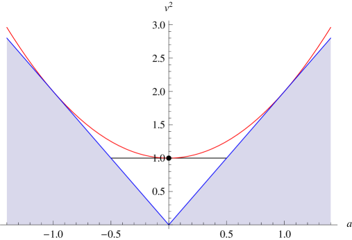
Figure 1: Solutions exist for all parameters inside the wedge. Solutions for parameters below the parabola are always real. Solutions for parameters above the parabola are complex in the Type II cases. The black dot represents Euclidean AdS₄, with round three-sphere boundary.

Two special loci correspond to the one-parameter solutions that appeared before in the literature. The $v^{2}$ axis, at $a=0$, corresponds to the Taub-NUT-AdS solutions in [8, 9]. In this case there are two inequivalent choices of $Q$ (up to signs), which correspond to the 1/4 BPS and 1/2 BPS instantons discussed in [9]. Notice the latter is real or pure imaginary depending on whether $v^{2}$ is smaller or larger than $1$. The segment at $v^{2}=1$, parameterised by $a\in[-\tfrac{1}{2},\tfrac{1}{2}]$, corresponds to the solution of [7]. To see this, one has to identify the parameters as $a=\tfrac{1}{2}\tfrac{b^{2}-1}{b^{2}+1}$, while the change coordinates between $\theta$ and $\vartheta$ may be obtained equating the respective functions $H(\theta)$ and $H(\vartheta)$. In this case, two values of $Q$ in (4.4) vanish, leaving only the (real) instanton discussed in [7].

5 Holographic free energy

In this section we compute the holographic free energy associated to our supergravity solutions using standard holographic renormalization methods [18, 19]. The total on-shell action is

$$I = I^{\text{grav}}_{\text{bulk}}+I^{F}+I^{\text{grav}}_{\text{ct}}+I^{\text{grav}}_{\text{bdry}}~{}.$$ (5.1)

Here the first two terms are the bulk supergravity action (2.1)

$$I^{\text{grav}}_{\text{bulk}}+I^{F} \equiv -\frac{1}{16\pi G_{4}}\int\mathrm{d}^{4}x\sqrt{g_{\mu\nu}}\left(R+6-F^{2}\right)~{},$$ (5.2)

evaluated on a particular solution. This is divergent, but we may regularize it using holographic renormalization. Introducing a cut-off at some large value of $q=\varrho$, with corresponding hypersurface $\mathcal{S}_{\varrho}=\{q=\varrho\}$, we add the following boundary terms

$$I^{\text{grav}}_{\text{ct}}+I^{\text{grav}}_{\text{bdry}} = \frac{1}{8\pi G_{4}}\int_{\mathcal{S}_{\varrho}}\mathrm{d}^{3}x\sqrt{\gamma_{\alpha\beta}}\left(2+\tfrac{1}{2}R(\gamma_{\alpha\beta})-K\right)~{}.$$ (5.3)

Here $R(\gamma)$ is the Ricci scalar of the induced metric $\gamma_{\mu\nu}$ on $\mathcal{S}_{\varrho}$, and $K$ is the trace of the second fundamental form of $\mathcal{S}_{\varrho}$, the latter being the Gibbons-Hawking boundary term. We compute

$$I^{\text{grav}}_{\text{bulk}} = \frac{\varpi}{8\pi G_{4}}\left[p_{3}p_{4}(p_{4}^{2}-p_{3}^{2})-(p_{4}^{3}-p_{3}^{3})\varrho+(p_{4}-p_{3})\varrho^{3}\right]~{},$$ (5.4)

$$I^{\text{grav}}_{\text{ct}}+I^{\text{grav}}_{\text{bdry}} = \frac{\varpi}{8\pi G_{4}}\left[M(p_{4}-p_{3})-(p_{4}-p_{3})\varrho^{3}+(p_{4}^{3}-p_{3}^{3})\varrho+O(\varrho^{-1})\right]~{}.$$

As expected, the divergent terms cancel as $\varrho\to\infty$. In the above expressions we have introduced

$$\varpi\ \equiv\ \int\mathrm{d}\sigma\mathrm{d}\tau\ =\ -16\pi^{2}\frac{p_{4}^{2}-p_{3}^{2}}{\mathcal{P}^{\prime}(p_{3})\mathcal{P}^{\prime}(p_{4})}~{},$$ (5.5)

where the integral is computed after writing $\tau,\sigma$ in terms of the coordinates $\varphi_{1},\varphi_{2}$. The contribution to the action of the gauge field is finite in all cases and does not need regularization. In particular, we have

$$I_{F} = Q^{2}\frac{\varpi}{8\pi G_{4}}\frac{p_{4}-p_{3}}{p_{4}+p_{3}}~{}.$$ (5.6)

Combining all the above contributions to the action we obtain the following expression:

$$I = \frac{\varpi}{8\pi G_{4}}\left[p_{3}p_{4}(p_{4}^{2}-p_{3}^{2})+M(p_{4}-p_{3})+Q^{2}\frac{p_{4}-p_{3}}{p_{4}+p_{3}}\right]~{}.$$ (5.7)

Substituting for $M=-\frac{1}{2}(p_{3}+p_{4})(p_{3}p_{4}-p_{1}p_{2})$ and $Q$ given in (3.31), we find the following values of the free energies

$$I = \frac{\pi}{2G_{4}}\begin{cases}1\\ \frac{(p_{3}+p_{4})^{2}}{(p_{4}-p_{1})(p_{3}-p_{2})}\\ \frac{(p_{3}+p_{4})^{2}}{(p_{3}-p_{1})(p_{4}-p_{2})}\end{cases}~{},$$ (5.8)

in the three cases, respectively. Finally, writing this in terms of the parameters $a$ and $v$, we obtain

$$I=\frac{\pi}{2G_{4}}\begin{cases}1\qquad\qquad\mathrm{Type~{}I}\\[5.69054pt] \frac{1}{1-4Q^{2}}\qquad\mathrm{Type~{}II}\end{cases}.$$ (5.9)

Remarkably, the free energy can always be expressed entirely in terms of $Q^{2}$. After the change of variables $Q=\frac{1}{2}\frac{\beta^{2}-1}{\beta^{2}+1}$, the free energy in the Type II case takes the familiar form

$$I=\frac{\pi}{8G_{4}}\left(\beta+\frac{1}{\beta}\right)^{2}~{},$$ (5.10)

where, definig $a=\frac{1}{2}\frac{b^{2}-1}{b^{2}+1}$, the parameter $\beta$ is given by

$$\beta^{2} = \frac{(1+b^{2})(2-v^{2})+\sqrt{(b^{2}-1)^{2}-4(v^{2}-1)(b^{2}+1)^{2}}}{1-b^{2}+v^{2}+b^{2}v^{2}}~{}.$$ (5.11)

When $v=1$ we have $b=\beta$, while when $b=1$, we have $\tfrac{2}{v}=\beta+\tfrac{1}{\beta}$, and one can check that the free energies reduce to those computed previously in the special cases.

6 Discussion

In this paper we constructed a family of rigid supersymmetric geometries depending on two parameters, comprising a deformed three-sphere and various background fields. These interpolate between all the previously known rigid supersymmetric geometries with topology of the three-sphere [5, 6]. ${\cal N}=2$ supersymmetric gauge theories may be placed on these backgrounds, with precise Lagrangians and supersymmetry transformation rules [1, 2], and we have presented supergravity solutions conjecturally dual to these. Although these were obtained in $d=4$, ${\cal N}=2$ gauged supergravity, using the results of [11] and [9], all our solutions may be uplifted to global supersymmetric solutions of (Euclidean) M-theory. We have computed the holographic free energy in the various cases, finding that it is either constant, or it depends on the parameters in a simple way, thus making a prediction for the large $N$ limit of the localized partition function of a large class of supersymmetric guage theories. This strongly suggests that the full localized partition function on these backgrounds may be written in terms of the double sine function $s_{\beta}(x)$, where in the Type I solutions $\beta=1$, while in the Type II solutions $\beta$ is given in (5.11). More generally, it suggests that on any supersymmetric geometry with $S^{3}$ topology, the partition function can be expressed in terms of $s_{\beta}(x)$, for an appropriate $\beta$. It would be interesting to understand better the geometric interpretation of this $\beta$.

Acknowledgments

We would like to thank James Sparks for collaboration at the initial stages of this work. D. M. is supported by an ERC Starting Grant – Grant Agreement N. 304806 – Gauge-Gravity, and also acknowledges partial support from an EPSRC Advanced Fellowship EP/D07150X/3 and from the STFC grant ST/J002798/1. A.P. is supported by an A.G. Leventis Foundation grant, an STFC studentship and via the Act “Scholarship Programme of S.S.F. by the procedure of individual assessment, of 2011-12” by resources of the Operational Programme for Education and Lifelong Learning, of the European Social Fund (ESF) and of the NSRF, 2007-2013.

Appendix A Integrability conditions

A.1 Integrability condition of the bulk Killing spinor equation

The integrability condition of (3.1) reads:

$$\frac{1}{4}R_{\mu\nu}{}^{ab}\Gamma_{ab}\epsilon+\frac{1}{2}\Gamma_{\mu\nu}\epsilon = \mathrm{i}F_{\mu\nu}\epsilon-\frac{\mathrm{i}}{2}\nabla_{[\mu}F_{|\,ab}\Gamma^{ab}_{\ \ |}\Gamma_{\nu]}\epsilon-\frac{\mathrm{i}}{4}\Gamma_{[\mu}F_{|\,ab}\Gamma^{ab}_{\ \ |}\Gamma_{\nu]}\epsilon$$ (A.1)

$$+\frac{1}{16}\left[F_{ab}\Gamma^{ab}\Gamma_{\mu},F_{cd}\Gamma^{cd}\Gamma_{\nu}\right]\epsilon-\frac{\mathrm{i}}{4}F_{ab}\Gamma^{ab}\Gamma_{\mu\nu}\epsilon~{}.$$

We shall use the above equation to obtain an algebraic relation between $\epsilon_{+}$ and $\epsilon_{-}$. We need to extract only one non-trivial component. In the orthonormal frame (3) we pick the $23$ component. Using

$$R_{2314}\ =\ \frac{M}{(p+q)^{3}}~{},~{}~{}~{}~{}~{}R_{2323}\ =\ -1-\frac{M}{(p+q)^{3}}$$ (A.2)

and

$$\nabla_{3}F_{14}\ =\ \nabla_{3}F_{32} = \frac{Q}{(p+q)^{3}}\sqrt{\frac{\mathcal{P}(p)}{p^{2}-q^{2}}}$$

$$\nabla_{2}F_{14}\ =\ \nabla_{2}F_{32} = -\frac{Q}{(p+q)^{3}}\sqrt{\frac{\mathcal{Q}(q)}{q^{2}-p^{2}}}$$ (A.3)

we derive

$$\epsilon_{+}=\Omega\;\epsilon_{-}~{},~{}~{}~{}~{}~{}\Omega\ =\ Q\begin{pmatrix}\frac{\mathrm{i}\sqrt{\frac{\mathcal{Q}(q)}{q^{2}-p^{2}}}}{M-(p+q)Q}&\frac{\sqrt{\frac{\mathcal{P}(p)}{p^{2}-q^{2}}}}{M-(p+q)Q}\\ \frac{-\sqrt{\frac{\mathcal{P}(p)}{p^{2}-q^{2}}}}{M+(p+q)Q}&\frac{-\mathrm{i}\sqrt{\frac{\mathcal{Q}(q)}{q^{2}-p^{2}}}}{M+(p+q)Q}\end{pmatrix}~{}.$$ (A.4)

A.2 Integrability condition of the boundary Killing spinor equation

The integrability condition of (3.14) reads:

$$\biggl{[}\frac{1}{4}R^{(3)}_{\alpha\beta\delta\epsilon}\gamma^{\delta\epsilon}-\mathrm{i}F^{(3)}_{\alpha\beta}+\mathrm{i}\partial_{[\alpha}p\gamma_{\beta]}-\frac{1}{2}p^{2}\gamma_{\alpha\beta}-2\mathrm{i}\nabla^{(3)}_{[\alpha|}V^{(3)}_{\delta}\gamma_{|\beta]}\gamma^{\delta}$$

$$+2p\gamma_{[\alpha}V^{(3)}_{\beta]}+2V^{(3)}{}^{\delta}V^{(3)}_{\delta}\gamma_{\alpha\beta}-4V^{(3)}_{\delta}\gamma_{[\alpha}V^{(3)}_{\beta]}\gamma^{\delta}\biggr{]}\,\chi = 0~{}.$$ (A.5)

In the orthonormal frame (3.16) we pick the $12$ component. Using

$$R^{(3)}_{1213} = -\sqrt{-\mathcal{P}(p)}$$

$$R^{(3)}_{1212} = 3p^{2}+E$$

$$\nabla_{1}^{(3)}V^{(3)}_{2}\ =\ -\nabla_{2}^{(3)}V^{(3)}_{1} = \frac{M}{2Q}p$$ (A.6)

we find

$$\Omega^{(3)}\chi = 0$$ (A.7)

where

$$\Omega^{(3)}\ =\ \begin{pmatrix}p^{2}-\frac{M}{Q}p-Q+\frac{1}{2}\left(\frac{M^{2}}{Q^{2}}+E\right)&-\mathrm{i}\sqrt{-\mathcal{P}(p)}\\ \mathrm{i}\sqrt{-\mathcal{P}(p)}&-p^{2}-\frac{M}{Q}p-Q-\frac{1}{2}\left(\frac{M^{2}}{Q^{2}}+E\right)\end{pmatrix}~{}.$$ (A.8)

In order for (A.7) to have a solution, the determinant

$$\det\Omega^{(3)} = \frac{1}{4}\left(\frac{M^{2}}{Q^{2}}+E\right)^{2}-\alpha$$ (A.9)

must be zero. Using the relations

$$E = p_{1}p_{2}+p_{1}p_{3}+p_{2}p_{3}+p_{1}p_{4}+p_{2}p_{4}+p_{3}p_{4}$$

$$M = \tfrac{1}{2}(p_{1}p_{2}p_{3}+p_{1}p_{2}p_{4}+p_{1}p_{3}p_{4}+p_{2}p_{3}p_{4})$$

$$\alpha = p_{1}p_{2}p_{3}p_{4}+Q^{2}$$

$$0 = p_{1}+p_{2}+p_{3}+p_{4}$$ (A.10)

we derive

$$\det\Omega^{(3)} = \frac{\alpha_{1}\alpha_{2}\alpha_{3}}{(8Q^{2})^{2}}~{},$$ (A.11)

where

$$\alpha_{1} = (p_{3}+p_{4})^{2}(p_{3}+p_{1})^{2}-4Q^{2}$$

$$\alpha_{2} = (p_{3}+p_{4})^{2}(p_{4}+p_{1})^{2}-4Q^{2}$$

$$\alpha_{3} = (p_{3}+p_{1})^{2}(p_{4}+p_{1})^{2}-4Q^{2}~{}.$$ (A.12)

Hence we obtain the following possibilities:

$$Q=\begin{cases}\pm\frac{(p_{3}+p_{1})(p_{4}+p_{1})}{2}\\ \pm\frac{(p_{3}+p_{4})(p_{3}+p_{1})}{2}\\ \pm\frac{(p_{3}+p_{4})(p_{4}+p_{1})}{2}\end{cases}~{}.$$ (A.13)

In addition, (A.7) relates $\chi^{-}$ and $\chi^{+}$ as

$$\chi^{+} = \sqrt{\frac{p^{2}+\frac{M}{Q}p+Q+\sqrt{\alpha}}{p^{2}-\frac{M}{Q}p-Q+\sqrt{\alpha}}}\,\chi^{-}~{},$$ (A.14)

which is equation (B.10) in the main text.

Appendix B More on the Killing spinors

In this appendix we discuss properties of the Killing spinors and some of their bilinears.

B.1 $\chi$, $\chi^{c}$ and $\tilde{\chi}$

We may write down the following three, in general distinct, Killing spinor equations:

$$\nabla_{\alpha}^{(3)}\chi-\mathrm{i}(A^{(3)}_{\alpha}+V^{(3)}_{\alpha})\chi+\tfrac{1}{2}H\gamma_{\alpha}\chi+\epsilon_{\alpha\beta\rho}V^{(3)}{}^{\beta}\gamma^{\rho}\chi = 0~{},$$ (B.1)

$$\nabla_{\alpha}^{(3)}\chi^{c}+\mathrm{i}(\bar{A}^{(3)}_{\alpha}+\bar{V}^{(3)}_{\alpha})\chi^{c}-\tfrac{1}{2}\bar{H}\gamma_{\alpha}\chi^{c}-\epsilon_{\alpha\beta\rho}\bar{V}^{(3)}{}^{\beta}\gamma^{\rho}\chi^{c} = 0~{},$$ (B.2)

$$\nabla_{\alpha}^{(3)}\tilde{\chi}+\mathrm{i}(A^{(3)}_{\alpha}+V^{(3)}_{\alpha})\tilde{\chi}+\tfrac{1}{2}H\gamma_{\alpha}\tilde{\chi}-\epsilon_{\alpha\beta\rho}V^{(3)}{}^{\beta}\gamma^{\rho}\tilde{\chi} = 0~{}.$$ (B.3)

Equation (B.2) is the charge conjugate of equation (B.1), where a bar in $\bar{A}^{(3)}$, $\bar{V}^{(3)}$, $\bar{H}$ denotes complex conjugation and the charge conjugate spinor $\chi^{c}$ is defined as

$$\chi^{c}\ =\ C\chi^{*}~{},~{}~{}~{}~{}~{}~{}~{}C\ =\ \begin{pmatrix}0&1\\ -1&0\end{pmatrix}~{}.$$ (B.4)

Notice that (B.2) is also obtained from (B.1) by replacing

$$A^{(3)}~{}\to~{}-\bar{A}^{(3)}~{},\qquad V^{(3)}~{}\to~{}-\bar{V}^{(3)}~{},\qquad H~{}\to~{}-\bar{H}~{},$$ (B.5)

and for any solution $\chi$ of (B.1), $\chi^{c}$ is a solution of (B.2). On the other hand, (B.3) is obtained from (B.1) by replacing

$$A^{(3)}~{}\to~{}-A^{(3)}~{},\qquad V^{(3)}~{}\to~{}-V^{(3)}~{},\qquad H~{}\to~{}H~{},$$ (B.6)

and in general is an independent equation. In particular, the existence of a solution $\chi$ to (B.1) does not imply that there exists a solution $\tilde{\chi}$ to (B.3). There are two special cases:

1. if $A^{(3)}$, $V^{(3)}$ are real and $H$ is pure imaginary then (B.2) and (B.3) coincide. In this case, for any solution $\chi$ to (B.1) there is also a solution $\tilde{\chi}=\chi^{c}$ to (B.3).

2. if $A^{(3)}$, $V^{(3)}$ and $H$ are pure imaginary then (B.1) and (B.2) coincide. In this case, for any solution $\chi$ to (B.1) there is also a second solution $\chi^{c}$ to (B.1). As in Euclidean signature $\chi$ and $\chi^{c}$ are independent, this implies that these configurations are 1/2 BPS.

Let us now discuss how our solutions fit into these relationships. We chose conventionally to refer to the solutions with a specific choice of signs of $Q$ (lower signs in (A.13)) as spinors $\chi$ solving (B.1). Namely, we take

$$\chi(Q)\ =\ \begin{pmatrix}\sqrt{w_{+}(p)}\\ \sqrt{w_{-}(p)}\end{pmatrix}\mathrm{e}^{\mathrm{i}\Phi(Q)}~{},$$ (B.7)

where

$$Q=\begin{cases}\frac{v^{2}-1}{2}\\[5.12149pt] \frac{1}{2}(\sqrt{a^{2}+1-v^{2}}+a)\\[5.12149pt] \frac{1}{2}(\sqrt{a^{2}+1-v^{2}}-a)\end{cases},\qquad\quad\Phi(Q)\ =\ \begin{cases}\frac{1}{2}(\varphi_{1}+\varphi_{2})\\[5.12149pt] \frac{1}{2}(-\varphi_{1}+\varphi_{2})\\[5.12149pt] \frac{1}{2}(\varphi_{1}-\varphi_{2})\end{cases}.$$ (B.8)

Then using the fact that under $Q\rightarrow-Q$ our background fields transform as in (B.6) and $w_{+}(p)\leftrightarrow w_{-}(p)$, $\Phi\rightarrow-\Phi$, it follows that

$$\tilde{\chi}(Q)\ \equiv\ \chi(-Q)\ =\ \begin{pmatrix}\sqrt{w_{-}(p)}\\ \sqrt{w_{+}(p)}\end{pmatrix}\mathrm{e}^{-\mathrm{i}\Phi(Q)}~{},$$ (B.9)

is a solution to (B.3), for all choices of $Q$ in (B.8).

Let us now look at the charge conjugate of (B.7). In general this reads

$$\chi^{c}(Q)\ =\ \begin{pmatrix}~{}\left(\sqrt{w_{-}(p)}\right)^{*}\\[5.12149pt] -\left(\sqrt{w_{+}(p)}\right)^{*}\end{pmatrix}\mathrm{e}^{-\mathrm{i}\Phi(Q)}~{}.$$ (B.10)

Equation (B.2) can be obtained from (B.1) transforming the fields as in (B.5), which in our solutions corresponds to

$$Q\ \to\ -Q^{*}~{}.$$ (B.11)

Therefore we should find that under (B.11) the spinor $\chi(Q)\to\chi^{c}(Q)$. Let us first assume that $Q\in\mathbb{R}$, then $\chi(Q)\to\tilde{\chi}(Q)$ as in (B.9) and we have

$$\chi^{c}(Q)\ =\ \begin{pmatrix}~{}\left(\sqrt{w_{-}(p)}\right)^{*}\\[5.12149pt] -\left(\sqrt{w_{+}(p)}\right)^{*}\end{pmatrix}\mathrm{e}^{-\mathrm{i}\Phi(Q)}\ =\ \pm\begin{pmatrix}\sqrt{w_{-}(p)}\\ \sqrt{w_{+}(p)}\end{pmatrix}\mathrm{e}^{-\mathrm{i}\Phi(Q)}=\pm\tilde{\chi}(Q)~{}.$$ (B.12)

Here we have used the fact that for $Q\in\mathbb{R}$, $w_{-}(p)$ and $w_{+}(p)$ are real and since $w_{-}(p)w_{+}(p)=\mathcal{P}(p)\leq 0$ it follows that either $w_{-}(p)\leq 0$, $w_{+}(p)\geq 0$ or $w_{-}(p)\geq 0$, $w_{+}(p)\leq 0$, resulting in the two signs above.

More generally, when $Q\in\mathbb{C}$, (B.11) implies that

$$\chi(Q)\ \to\ \chi(-Q^{*})=\begin{pmatrix}\sqrt{w_{-}(p)^{*}}\\ \sqrt{w_{+}(p)^{*}}\end{pmatrix}\mathrm{e}^{-\mathrm{i}\Phi(Q)}~{},$$ (B.13)

where we used the fact that the two (lower) Type II cases of $Q$ in (B.8) are exchanged under (B.11). In order to compare (B.13) to (B.10) we must use the fact that

$$w_{+}(p)=|w_{+}(p)|\mathrm{e}^{\mathrm{i}\varphi_{+}(p)}~{},~{}w_{-}(p)=|w_{-}(p)|\mathrm{e}^{\mathrm{i}\varphi_{-}(p)}~{},~{}~{}\mathrm{with}~{}~{}\varphi_{+}(p)+\varphi_{-}(p)=\pi~{}.$$ (B.14)

One can then check that in order for (B.13) to agree (up to a possible sign depending on the signs of Re$[w_{\pm}(p)]$) with (B.10) one should define the square root on the complex plane with a branch cut along the positive imaginary axis. This definition would fail to give the correct relation for purely imaginary values of $w_{\pm}(p)$, but this of course cannot happen.

We have therefore shown that the two solutions of Type II are just charge conjugate to each other. A special case arises when $Q$ is purely imaginary, which we discuss below.

B.2 Coordinate $\theta$ and the $a=0$ case

To write the spinors in the coordinate $\theta$ one should make the coordinate transformation $p=\frac{1}{2}-a\cos\theta$ and then substitute into (B.7) the following

$$\left\{\begin{array}[]{ccl}w_{+}(\theta)&=&-a^{2}\sin^{2}\theta\\ w_{-}(\theta)&=&(a\cos\theta-1)^{2}+2Q-a^{2}\end{array}\right.~{}~{}\mathrm{for}~{}Q=\frac{v^{2}-1}{2}~{},$$ (B.17)

in the Type I solutions and

$$w_{\pm}(\theta)\ =\ \begin{cases}a(\cos\theta\pm 1)(a\cos\theta-1\mp 2Q\pm a)\\ a(\cos\theta\mp 1)(a\cos\theta-1\mp 2Q\mp a)\\ \end{cases}~{}~{}\mathrm{for}~{}Q\ =\ \begin{cases}\tfrac{1}{2}(\sqrt{a+1-v^{2}}+a)\\ \tfrac{1}{2}(\sqrt{a+1-v^{2}}-a)\end{cases}$$ (B.18)

in the type II solutions. Although the resulting expressions are not particularly simple, it is now possible to take the limit $a\to 0$. The Type I spinor then reduces to

$$\chi_{a=0}\ =\ \begin{pmatrix}0\\ v\end{pmatrix}\mathrm{e}^{\tfrac{\mathrm{i}}{2}(\varphi_{1}+\varphi_{2})}~{},$$ (B.19)

that is the spinor of the 1/4 BPS biaxially squashed three-sphere [9]. Upon rescaling $w_{\pm}(\theta)\rightarrow w_{\pm}(\theta)/a$ before taking the $a\to 0$, the Type II spinors instead reduce to

$$\chi_{a=0}\ =\ \begin{pmatrix}\cos\frac{\theta}{2}\\ \mathrm{i}\sin\frac{\theta}{2}\end{pmatrix}\mathrm{e}^{\tfrac{\mathrm{i}}{2}(-\varphi_{1}+\varphi_{2})}~{},\qquad\chi^{c}_{a=0}\ =\ \begin{pmatrix}\mathrm{i}\sin\frac{\theta}{2}\\ \cos\frac{\theta}{2}\end{pmatrix}\mathrm{e}^{\tfrac{\mathrm{i}}{2}(\varphi_{1}-\varphi_{2})}~{},$$ (B.20)

up to irrelevant constants. These are the two spinors of the 1/2 BPS biaxially squashed three-sphere [9]. Notice that indeed they are charge conjugate to each other. Moreover, when $v^{2}>1$, $Q$ is pure imaginary, and it follows from the discussion above that they are both solutions to (B.1).

B.3 Spinor bilinears

We evaluate the bilinears $K_{\alpha}=\chi\gamma_{\alpha}\tilde{\chi}$ and $\rho_{\alpha}\ =\ \chi\gamma_{\alpha}\chi$ appearing in [2] for our solutions. The contraction of two spinors is defined as

$$\psi\zeta\ =\ C^{\alpha\beta}\psi_{\beta}\zeta_{\alpha}~{}.$$ (B.21)

We have

$$K = 2\left[(p^{2}+\sqrt{\alpha})(p_{3}^{2}-p^{2})+\mathcal{P}(p)\right]\mathrm{d}\phi_{1}+2\left[(p^{2}+\sqrt{\alpha})(p_{4}^{2}-p^{2})+\mathcal{P}(p)\right]\mathrm{d}\phi_{2}~{},$$

$$\rho = \frac{-2\mathrm{e}^{2\mathrm{i}\Phi}}{\sqrt{-\mathcal{P}(p)}}\left[(\tfrac{M}{Q}p+Q)\mathrm{d}p+\mathrm{i}\,\mathcal{P}(p)[(p_{3}^{2}-\sqrt{\alpha})\mathrm{d}\phi_{1}+(p_{4}^{2}-\sqrt{\alpha})\mathrm{d}\phi_{2}]\right]~{},$$ (B.22)

where recall that $\phi_{1}=\frac{2}{\mathcal{P}^{\prime}(p_{3})}\varphi_{1}$ and $\phi_{2}=\frac{2}{\mathcal{P}^{\prime}(p_{4})}\varphi_{2}$. The dual Killing vector field is

$$K^{\sharp}\ =\ \frac{\sqrt{\alpha}+p_{4}^{2}}{p_{3}^{2}-p_{4}^{2}}\mathcal{P}^{\prime}(p_{3})\partial_{\varphi_{1}}-\frac{\sqrt{\alpha}+p_{3}^{2}}{p_{3}^{2}-p_{4}^{2}}\mathcal{P}^{\prime}(p_{4})\partial_{\varphi_{2}}~{}.$$ (B.23)

Notice that $K$, $K^{\sharp}$ are in general complex. They become real if and only if $\sqrt{\alpha}\in\mathbb{R}$, which can happen only when $Q$ is purely real or imaginary, as for the special cases previously studied in the literature. Both $K$ and $\rho$ are globally defined one-forms on the three-sphere. Furthermore, $\rho$ satisfies the condition [1, 2] $\rho\wedge\mathrm{d}\rho=0$.

References

- [1] C. Klare, A. Tomasiello and A. Zaffaroni, “Supersymmetry on Curved Spaces and Holography,” JHEP 1208, 061 (2012) [arXiv:1205.1062 [hep-th]].
- [2] C. Closset, T. T. Dumitrescu, G. Festuccia and Z. Komargodski, “Supersymmetric Field Theories on Three-Manifolds,” JHEP 1305, 017 (2013) [arXiv:1212.3388].
- [3] G. Festuccia and N. Seiberg, “Rigid Supersymmetric Theories in Curved Superspace,” JHEP 1106, 114 (2011). [arXiv:1105.0689 [hep-th]].
- [4] M. F. Sohnius and P. C. West, “An Alternative Minimal Off-Shell Version of N=1 Supergravity,” Phys. Lett. B 105, 353 (1981).
- [5] N. Hama, K. Hosomichi and S. Lee, “SUSY Gauge Theories on Squashed Three-Spheres,” JHEP 1105, 014 (2011) [arXiv:1102.4716 [hep-th]].
- [6] Y. Imamura and D. Yokoyama, “ supersymmetric theories on squashed three-sphere,” Phys. Rev. D 85, 025015 (2012) [arXiv:1109.4734 [hep-th]].
- [7] D. Martelli, A. Passias and J. Sparks, “The gravity dual of supersymmetric gauge theories on a squashed three-sphere,” Nucl. Phys. B 864 (2012) 840 [arXiv:1110.6400 [hep-th]].
- [8] D. Martelli and J. Sparks, “The gravity dual of supersymmetric gauge theories on a biaxially squashed three-sphere,” Nucl. Phys. B 866, 72 (2013) [arXiv:1111.6930 [hep-th]].
- [9] D. Martelli, A. Passias and J. Sparks, “The supersymmetric NUTs and bolts of holography,” To be published in Nucl. Phys. B arXiv:1212.4618 [hep-th].
- [10] D. Z. Freedman, A. K. Das, “Gauge Internal Symmetry in Extended Supergravity,” Nucl. Phys. B120, 221 (1977).
- [11] J. P. Gauntlett, O. Varela, “Consistent Kaluza-Klein reductions for general supersymmetric AdS solutions,” Phys. Rev. D76, 126007 (2007). [arXiv:0707.2315 [hep-th]].
- [12] J. P. Gauntlett, S. Kim, O. Varela, D. Waldram, “Consistent supersymmetric Kaluza-Klein truncations with massive modes,” JHEP 0904, 102 (2009). [arXiv:0901.0676 [hep-th]].
- [13] J. F. Plebanski and M. Demianski, “Rotating, charged, and uniformly accelerating mass in general relativity,” Annals Phys. 98, 98 (1976).
- [14] D. Martelli and J. Sparks, “Resolutions of non-regular Ricci-flat Kähler cones,” J. Geom. Phys. 59, 1175 (2009) [arXiv:0707.1674 [math.DG]].
- [15] N. Alonso-Alberca, P. Meessen and T. Ortin, “Supersymmetry of topological Kerr-Newman-Taub-NUT-AdS space-times,” Class. Quant. Grav. 17 (2000) 2783 [arXiv:0003071[hep-th]].
- [16] D. Klemm and M. Nozawa, “Supersymmetry of the C-metric and the general Plebanski-Demianski solution,” JHEP 1305, 123 (2013) [arXiv:1303.3119 [hep-th]].
- [17] K. Behrndt, G. Dall’Agata, D. Lust and S. Mahapatra, “Intersecting six-branes from new seven manifolds with holonomy,” JHEP 0208, 027 (2002) [arXiv:0207117[hep-th]].
- [18] R. Emparan, C. V. Johnson and R. C. Myers, “Surface terms as counterterms in the AdS / CFT correspondence,” Phys. Rev. D 60, 104001 (1999) [hep-th/9903238].
- [19] K. Skenderis, “Lecture notes on holographic renormalization,” Class. Quant. Grav. 19, 5849 (2002) [hep-th/0209067].
- [20] L. F. Alday, D. Martelli, P. Richmond and J. Sparks, “Localization on Three-Manifolds,” arXiv:1307.6848 [hep-th].