Review of Recent Neutrino Physics Research

Abstract

We review recent research in neutrino physics, including neutrino oscillations to test time reversal and CP symmetry violations, the measurement of parameters in the U matrix, sterile neutrino emission causing pulsar kicks, and neutrino energies in the neutrinosphere.

PACS Indices:12.38.Aw,13.60.Le,14.40.Lb,14.40Nd

1 Table of Contents

The Topics Reviewed Are:

Quantum States, Symmetries, Neutrino Oscillations

Time Reversal Violation (TRV) for Various Energies

and Baselines

A Proposed TRV experiment

CP Violation (CPV) for Various Energies

and Baselines

The LBNE Projct, CP and $\delta_{CP}$

Extracting $\theta_{13}$ Via Reactor Experiments

New Experimental and Theoretical Results

for Sterile Neutrinos and Pulsar Kicks

Neutrino Effective Masses in a Neutrinosphere

2 HAMILTONIAN, QUANTUM STATES, ENERGY EIGENSTATES, SYMMETRIES

We now review some basic quantum theory needed to obtain the time dependence of energy eigenstates, needed for neutrino oscillations and discrete symmetries, which are tested by neutrino oscillations.

2.1 Hamiltonian and Energy Eigenstates

In quantum theory one deals with states and operators. A quantum state represents a system, and a quantum operator operates on a state.

The Hamiltonian = $H$ is an operator. Consider a state $A$ in space-time: $|A(\vec{r},t)>$,

$$H|A(\vec{r},t)> = i(\partial/\partial t)|A(\vec{r},t)>\;.$$ (1)

If the state $|A>$ is an eigenstate of the operator $A$, $A|A>=a|A>$, where a is a constant, the value of $A$ in the state $|A>$. An energy eigenstate is an eigenstate of $H$:

$$H|A> = E_{A}|A>\;,$$ (2)

where $E_{A}$=energy, and $|A>$ is an energy eigenstate. In space-time

$$|A(\vec{r},t)> = e^{-iE_{A}t}|A(\vec{r})>\;,$$ (3)

since $He^{-iE_{A}t}|A(\vec{r})>=i(\partial/\partial t)e^{-iE_{A}t}|A(\vec{r})>=E_{A}e^{-iE_{A}t}|A(\vec{r})>$.

2.2 Discrete Symmetries:

The discrete symmetries that we deal with are parity, charge conjugation, and time reversal, with operators $P,C,{\rm\;and\;}T$.

The parity operator is defined by

$$P|A(\vec{r},t)> = \eta_{p}|A(-\vec{r},t)>\;,$$ (4)

with $|\eta_{p}|=1$. The charge conjugation operator is defined by

$$C|{\rm particle}> = \eta_{c}|\rm anti-particle>\;,$$ (5)

with $|\eta_{c}|=1$.

If the Hamiltonian is invariant under time reversal, $THT^{\dagger}=H$, then

$$Te^{-iH(t_{2}-t_{1})}T^{\dagger} = e^{-iH(t_{1}-t_{2})}\;.$$ (6)

The CPT Theorem: If the Lagrangian is local, $L=L(x^{\mu})$, and invariant to Lorentz Transformations CPT is conserved, so TRV =CPV in magnitude, where TRV is time reversal violation and CPV is CP (operator C $\times$ operator P) violation.

T and CP violations in neutrino oscillations have long been of interest, see Ref[1] for definitions and notation. For matter effects see Ref[2].

2.3 Neutrino Oscillations

Neutrinos are produced (e.g. by proton-proton collisions) with a flavor, the three flavors being electron, muon, tau neutrinos. They have no definite mass. As we now show, this leads to Neutrino Oscillations. We use units for which c=h=1, with c= the speed of light and h=Plank’s constant.

A neutrino with mass $m_{i}$ at rest ($E_{i}=m_{i}$) has t-dependence $|\nu_{i},t>=e^{-im_{i}t}|\nu_{i}>$. A neutrino with flavor a is related to the mass neutrino eigenstates, $\alpha$=1,2,3 by

$$\nu_{a} = U\nu_{\alpha}\;,$$

with the unitary transformation, U

$$U=\left(\begin{array}[]{lcr}c_{12}c_{13}&s_{12}c_{13}&s_{13}e^{-i\delta_{CP}}\\ -s_{12}c_{23}-c_{12}s_{23}s_{13}e^{i\delta_{CP}}&4c_{12}c_{23}-s_{12}s_{23}s_{13}e^{i\delta_{CP}}&s_{23}c_{13}\\ s_{12}s_{23}-c_{12}c_{23}s_{13}e^{i\delta_{CP}}&-c_{12}s_{23}-s_{12}c_{23}s_{13}e^{i\delta_{CP}}&c_{23}c_{13}\end{array}\right)\;.$$ (10)

The parameters are angles $\theta_{ij}$, (i,j) = (1,2), (1,3), (23), with $s_{ij}\equiv sin(\theta_{ij}),c_{ij}\equiv cos(\theta_{ij})$; and the angle $\delta_{CP}$.

Therefore, the electron neutrino state is related to the mass neutrino states by $|\nu_{e}>=\sum_{i}U_{ei}|\nu_{i}>$ and the time dependence of electron neutrinos at rest isc $|\nu_{e},t>=\sum_{i}U_{ei}|\nu_{i},t>=\sum_{i}U_{ei}e^{-im_{i}t}|\nu_{i}>$ Since the three neutrino masses are different, one finds $|\nu_{e},t>=c_{e}(t)|\nu_{e}>+c_{\mu}(t)|\nu_{\mu}>+c_{\tau}(t)|\nu_{\tau}>$, where $c_{f}(t)$ give the amplitude of flavor f for time t. There are similar relations for the mu and tau neutrinos.

From this one sees that as neutrinos travel they oscillate into neutrinos with a different flavor.

3 T, CP, CPT Violation and Neutrino Oscillations

Defining $P(\nu_{\alpha}\rightarrow\nu_{\beta})$ = transition probability of flavor $\alpha$ to flavor $\beta$ neutrino, the T, CP, and CPT violating probability differences are defined as (with $\bar{\nu}$ an anti-$\nu$:

$$\Delta P^{T}_{\alpha\beta} = P(\nu_{\alpha}\rightarrow\nu_{\beta})-P(\nu_{\beta}\rightarrow\nu_{\alpha})$$

$$\Delta P^{CP}_{\alpha\beta} = P(\nu_{\alpha}\rightarrow\nu_{\beta})-P(\bar{\nu}_{\alpha}\rightarrow\bar{\nu}_{\beta})$$

$$\Delta P^{CPT}_{\alpha\beta} = P(\nu_{\alpha}\rightarrow\nu_{\beta})-P(\bar{\nu}_{\beta}\rightarrow\bar{\nu}_{\alpha})\;,$$

where $\alpha,\beta=e,\mu,\tau$

The time evolution matrix, $S(t,t_{0})$, is used to derive $\Delta P^{T}_{ab}$:

$$|\nu(t)> = S(t,t_{0})|\nu(t_{0})>$$

$$i\frac{d}{dt}S(t,t_{0}) = H(t)S(t,t_{0})\;,$$

In the vacuum

$$S_{ab}(t,t_{0}) = \sum_{j=1}^{3}U_{aj}exp^{iE_{j}(t-t_{0})}U^{*}_{bj}$$ (11)

The neutrino-electron potential for neutrinos traveling through matter for matter density $n_{e}$ =3 gm/cc is

$$V = \sqrt{2}G_{F}n_{e}=1.13\times 10^{-13}{\rm\;eV}$$

where $G_{F}$ is the universal weak interaction Fermi constant. Note $P(\nu_{\alpha}\rightarrow\nu_{\beta})=|S_{\beta\alpha}|^{2}$; and $P(\bar{\nu}_{\alpha}\rightarrow\bar{\nu}_{\beta})=|\bar{S}_{\beta\alpha}|^{2}$ with $V\rightarrow-V$. I.e., $V$(anti-neutrinos)=-$V$(neutrinos).

3.1 Time Reversal in Neutrino Oscillations

This discussion of TRV is based on Ref[3], in which the formalism of Freund[17] is used.

The TRV electron-muon probability difference in matter is

$$\Delta P^{T}_{e\mu} = |S_{21}|^{2}-|S_{12}|^{2}$$

$$S_{12} = c_{23}\beta-is_{23}aA_{a}$$

$$S_{21} = -(c_{23}\beta+is_{23}aC_{a})$$

$$a = s_{13}(\Delta-s_{12}\delta)$$

$$\Delta P^{T}_{e\mu} = -2s_{13}s_{23}c_{23}(\Delta-s_{12}\delta)Im[e^{-i\delta_{CP}}\beta^{*}(A_{a}-C_{a}^{*})]\;,$$ (12)

with

$$A_{a} \simeq f(t,t_{0})I_{\alpha}*(t,t_{0})$$ (13)

$$I_{\alpha}*(t,t_{0}) = \int_{t_{0}}^{t}dt^{\prime}\alpha^{*}(t^{\prime},t)f(t^{\prime},t)$$

$$\alpha(t,t_{0}) = cos\omega(t-t_{0})-isin(2\theta)sin\omega(t-t_{0})$$

$$f(t,to) = e^{-i\Delta(t-t_{0})}$$

$$2\omega = \sqrt{\delta^{2}+V^{2}-2\delta Vcos(2\theta_{12})}$$

$$\beta = -isin2\theta sin\omega L$$

$$C_{a} = A_{a}$$

$$cos(2\theta) = \frac{\delta cos(2\theta_{12})-V}{2\omega}\;.$$

We choose $s_{13}=.187$, $s_{23}=c_{23}=.707$, $\theta_{12}=32^{o}$. Note $\delta=\delta m_{12}^{2}/(2E)\ll\Delta=\delta m_{13}^{2}/(2E)$ From $\Delta P^{T}_{e\mu}=|S_{21}|^{2}-|S_{12}|^{2}$ it follows that

$$\Delta P^{T}_{e\mu} = -2s_{13}s_{23}c_{23}(\Delta-s_{12}\delta)Im[e^{-i\delta_{CP}}\beta^{*}(A_{a}-C_{a}^{*})]$$

$$A_{a}-C_{a}^{*} = 2iIm[A_{a}]\simeq i\frac{2}{\Delta}[cos\Delta L-cos\omega L]{\rm\;,\;therefore,}$$ (14)

$$\Delta P^{T}_{e\mu} \simeq -4s_{13}s_{23}c_{23}sin\omega Lsin2\theta(cos\Delta L-cos\omega L)$$

$$\simeq 0.374sin\omega Lsin2\theta(cos\omega L-cos\Delta L)\;.$$

$\Delta P^{T}_{e\mu}$ is shown as a function of L for E=1 , a function of E for L=735 km

Note that for E= 1 GeV and L=735km (Minos parameters) TRV is approxmately 3%, which could be measured if muon as well as electron neutrino beams were available. Unfortunately, this is not now possible.

3.2 Proposed TRV Experiment

Since none of the neutrino oscillation facilities have beams of both $\nu_{e}$ and $\nu_{\mu}$ beams, with $\Delta P^{T}_{e\mu}=P(\nu_{e}\rightarrow\nu_{\mu})-P(\nu_{\mu}\rightarrow\nu_{e})$ the time reversal violation (TRV) probability, it is not possible to measure TRV at the present time. Recently a TRV experiment was proposed[5]. The proposed experiment is shown in Fig. 1. The neutrino beam is aimed at a new detector at the surface of the earth 735 km past the Soudan mine (position 3 in the figure), only a small deviation from the present MINOS neutrino beam (position 1). There would be a 1% increase in the electron neutrino probability that one would obtain with the 10% muon neutrino flux at the position of the Soudan mine. This would be a means for the measurement of TRV. Soudan mine. This would be a means for the measurement of TRV.

Figure 1: The present Minos neutrino beam and a proposed beam

3.3 CPV via Neutrino Oscillations

We start with an overview of CP and CV Violation (CPV)

CPV has a long history:

$K^{0}_{L}\rightarrow\pi^{+}+\pi^{-}$[6]

$K^{0}_{L}\rightarrow 2\pi^{0}$[7]

$K^{0}_{L}\rightarrow\pi^{0}+\nu+\bar{\nu}$[8]

The first study in the present work is an estimate the $\nu_{\mu}$ to $\nu_{e}$ conversion probability using parameters for the baseline and energy corresponding to MiniBooNE, JHF-Kamioka, MINOS, and CHOOZ-Double Cho0z, which are on-going projects, although the CHOOZ project does not have a beam of $\nu_{\mu}$ neutrinos.The two main parameters of interest in the present work are $\delta_{CP}$, which is essentially unknown, and $\theta_{13}$.

The LBNE Project, where neutrino beams produced at Fermilab with a baseline of L $\simeq$ 1200 km would be detected with deep underground detectors, has been proposed for studying CPV and the $\delta_{CP}$ parameter. We discuss the recent work on this project.

Next are shown results for $\mathcal{P}(\nu_{\mu}\rightarrow\nu_{e})$ for MiniBooNE, JHF-Kamioka, MINOS, Chooz parameters as a guide for future CPV experiments.

The angle $\theta_{13}$ will be measured by the Daya Bay experiment in China, the Double Chooz project in France, and RENO in Korea, via $\bar{\nu}_{e}$ disappearance. $\bar{\nu}_{e}$ disappearance is derived using the recent result from the Daya Bay project that $s_{13}\simeq 0.15$ as a test of the equation used by the Daya Bay experimental group compared to the more modern S-Matrix theory. It is shown that for some baselines it would be important to use the more modern theory.

Finally, using the expected range of values for $\theta_{13}$, CPV is estimated for $\mu-e$ neutrino oscillation for the entire range of $\delta_{CP}$ to help in the planning for future CPV experiments.

3.4 CP VIOLATION AND THE LBNE PROJECT

The two main objectives of the LBNE Project are to measure the $\delta_{CP}$ parameter and CPV via neutrino oscillations.

A study of CPV using the baseline (L=1200 km) and energies expected for the future LBNE Project, calculating CPV as a function of $\delta_{CP}$ was carried out[9] to help in the design of the project. An essential aspect of the determination of CPV is the interaction of neutrinos with matter as they travel along the baseline.

The CPV probability differences (note that the C operator changes a particle to its antiparticle) are defined as $\Delta P^{CP}_{ab}$

$$\Delta P^{CP}_{ab} = P(\nu_{a}\rightarrow\nu_{b})-P(\bar{\nu}_{a}\rightarrow\bar{\nu}_{b})\;.$$

In our present work we study $P(\nu_{\mu}\rightarrow\nu_{e})$ and $P(\bar{\nu}_{\mu}\rightarrow\bar{\nu}_{e})$, since the neutrino beams at MiniBooNE, JHF-Kamaoka, MINOS, and LBNE, as well as most other experimental facilities, are muon or anti-muon neutrinos.

The probability of CPV for $\mu,e$ neutrinos, $\Delta\mathcal{P}^{CP}_{\mu e}$ is

$$\Delta P^{CP}_{\mu e} = P(\nu_{\mu}\rightarrow\nu_{e})-P(\bar{\nu}_{\mu}\rightarrow\bar{\nu}_{e})$$

$$= |S_{12}|^{2}-|\bar{S}_{12}|^{2}$$

$$S_{12} = c_{23}\beta-is_{23}ae^{-i\delta_{CP}}A_{a}$$

$$\bar{S}_{12} = c_{23}\bar{\beta}-is_{23}ae^{i\delta_{CP}}\bar{A_{a}}\;,$$

with $c_{23},s_{23},\beta,A_{a}$ defined above. We use $s_{12}=0.56$ and $s_{23}=0.707$; and choose $s_{13}=0.19$, which one of the past projects found. Using the matter density $\rho$=3 gm/cc, $V=1.13\times 10^{-13}$. Note that for antineutrinos $\delta_{CP}\rightarrow-\delta_{CP}$. $\bar{\beta}=\beta(V\rightarrow-V)$ and $\bar{A}=A(V\rightarrow-V)$.

Note that if $V=0$, (vacuum), CPT is always conserved for normal theories, but for $V=\neq 0$ CP an T symmetries are independent

Using conservation of probabiltiy, $|A_{a}|^{2}=|\bar{A_{a}}|^{2}$, one finds (we do not give the rather complicated result here. See Ref[9]).

$$\Delta P^{CP}_{\mu e} = c_{23}^{2}(|\beta|^{2}-|\bar{\beta}|^{2})-2c_{23}s_{23}aIm[\beta e^{-i\delta_{CP}}A^{*}-e^{i\delta_{CP}}\bar{\beta}\bar{A}^{*}]\;.$$

The estimates of $\Delta P^{CP}_{\mu e}$ for the baseline and energies expected for the LBNE Project are shown in Fig. 2.

3.5 CONCLUSIONS FOR LBNE PROPOSED PROJECT:

In the LBNE Report (V. Barger $et\;al$, Report of the US long baseline neutrino experiment study (arXiv:0705.4396) results of extensive studies have shown that future experiments can extend our knowledge of neutrino oscillations beyond present and planned experiments. Since there will be both $\nu_{\mu}$ and $\bar{\nu}_{\mu}$ beams, the LBNE Project can test CPV.

We have estimated CP violation for the LBNE Project, with a baseline L=1200 km as a function of $\delta_{CP}$ for $\delta_{CP}$ = 0 to $\pi/2$ for energies of 1, 2, and 3 GeV. CPV over 3% was found with $\delta_{CP}=\pi/2$ for some energies, which the LBNE Project should be able to measure. Even for $\delta_{CP}=0$, for which CPV is entirely a matter effect, CPV probabilities of over 1% were found for E= 1 GeV, so the LBNE Project should be able to measure CPV for any expected values of $\delta_{CP}$.

We believe that these calculations should be useful in planning the future LBNE Project.

$\Delta P^{CP}_{\mu e}(E,\delta_{CP})$ as a function of $\delta_{CP}$ for energies E= 1, 2, 3 GeV, are shown in the figure.

Figure 2: The ordinate is $\Delta\mathcal{P}(\nu_{\mu}\rightarrow\nu_{e})$ for LBNE(L=1200 km), Energy=E in GeV, as a function of $\delta_{CP}$

3.6 CPV via Neutrino Oscillation in Matter and Parameters $s_{13},\delta_{CP}$

[L.S. Kisslinger, E.M. Henley, M.B. Johnson; arXiv:1203.6613/hep-ph; Int. J. of Mod. Phys. E 21, 1250065 (2012)]

An estimate of the dependence of $\nu_{\mu}$ to $\nu_{e}$ conversion on parameters $\theta_{13}$ and $\delta_{CP}$ for experimental facilities studying neutrino oscillations was carried out[10]. Of particular interest is the dependence on $\delta_{CP}$

Reactor experiments at Daya Bay, Double Chooz, and RENO measuring $\bar{\nu_{e}}$ disappearance are in progress, with the objective of determining $\theta_{13}$, an essential parameter for neutrino oscillations, to 1%

The S-Matrix theory is used to estimate $\bar{\nu_{e}}$ disappearance and compare estimates based on an older theory being used by Daya Bay, etc., experimentalists to extract $\theta_{13}$, using values of $\theta_{13}$ within known limits to estimate the dependence of $\nu_{\mu}$ - $\nu_{e}$ CPV probability on $\delta_{CP}$ in order to suggest new experiments to measure CPV for neutrinos moving in matter.

The transition probability $P(\nu_{\mu}\rightarrow\nu_{e})$ is obtained from $S_{12}$:

$$P(\nu_{\mu}\rightarrow\nu_{e}) = |S_{12}|^{2}=Re[S_{12}]^{2}+Im[S_{12}]^{2}\;,$$

with $S_{12}=c_{23}\beta-is_{23}ae^{-i\delta_{CP}}A_{a}$. Since $\delta=\delta m_{12}^{2}/(2E)$ and $\Delta=\delta m_{13}^{2}/(2E)$, $\delta\ll\Delta$; and one can show that

$$Re[S_{12}] = s_{23}a[cos(\bar{\Delta}L+\delta_{CP})Im[I_{\alpha*}]-sin(\bar{\Delta}L+\delta_{CP})Re[I_{\alpha*}]$$

$$Im[S_{12}] = -c_{23}sin2\theta sin\omega L-s_{23}a[cos(\bar{\Delta}L+\delta_{CP})Re[I_{\alpha*}]$$

$$+sin(\bar{\Delta}L+\delta_{CP})Im[I_{\alpha*}]]\;,$$

and $Re[I_{\alpha*}]\simeq\frac{sin\bar{\Delta}L}{\bar{\Delta}};Im[I_{\alpha*}]\simeq\frac{1-cos\bar{\Delta}L}{\bar{\Delta}}$.

From this one obtains the mu to e neutrino oscillation probability

$$P(\nu_{\mu}\rightarrow\nu_{e}) \simeq (c_{23}s_{12}c_{12}(\delta/\omega)sin\omega L)^{2}+2(s_{23}s_{13})^{2}(1-cos\bar{\Delta}L)$$

$$+2s_{13}s_{12}c_{12}s_{23}c_{23}(\delta/\omega)sin\omega L$$

$$(cos(\bar{\Delta}L+\delta_{CP})sin\bar{\Delta}L+sin(\bar{\Delta}L+\delta_{CP})(1-cos\bar{\Delta}L))\;.$$

Both $s_{13}$=.19 and .095 were used to show the effect of $s_{13}$.

The results for $P(\nu_{\mu}\rightarrow\nu_{e})$ are shown in Fig.3. These results can provide guidance for future experiments on CPV via $\nu_{\mu}\leftrightarrow\nu_{e}$ oscillation.

We calculated $P(\nu_{\mu}\rightarrow\nu_{e})$ for $\delta_{CP}$ from -$\pi$/2 to $\pi$/2, and the results are almost independent of $\delta_{CP}$. The results for CHOOZ are shown in preparing for the following subsection on $\bar{\nu_{e}}$ disappearance, even though Double Chooz, Daya Bay, and RENO projects have beams of $\bar{\nu}_{e}$ rather than $\nu_{\mu}$ neutrinos.

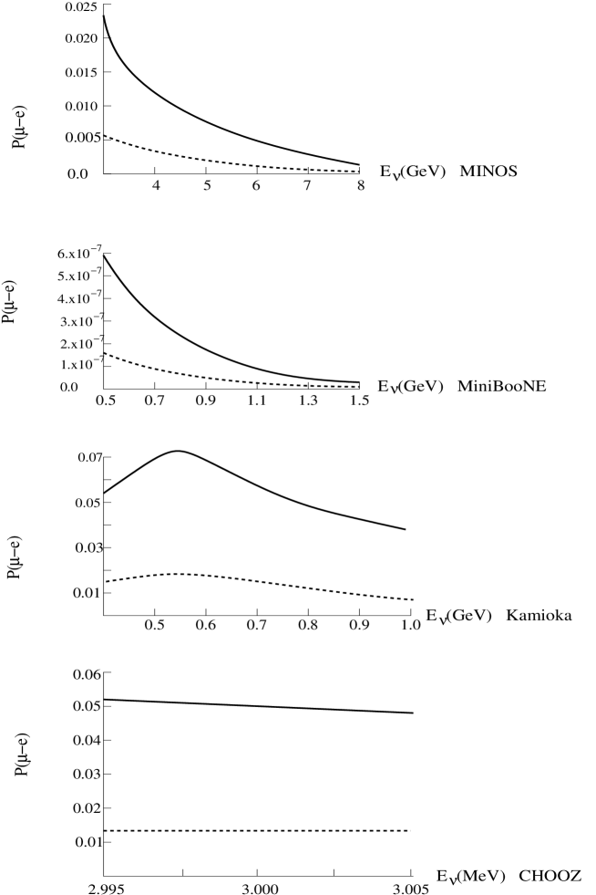
Figure 3:       The ordinate is $P(\nu_{\mu}\rightarrow\nu_{e})$ for MINOS(L=735 km), MiniBooNE(L=500m), JHF-Kamioka(L=295 km), and CHOOZ(L=1.03 km).       Solid curve for $s_{13}$=.19 and dashed curve for $s_{13}$=.095. The curves are almost independent of $\delta_{CP}$.

3.7 $\bar{\nu_{e}}$ DISAPPEARANCE DERIVED USING S-MATRIX THEORY COMPARED TO Daya Bay EVALUATION:

We derive $\bar{\nu_{e}}$ disappearance, $P(\bar{\nu}_{e}\rightarrow\bar{\nu}_{e})$, defined as

$$P(\bar{\nu}_{e}\rightarrow\bar{\nu}_{e}) = 1-P(\bar{\nu}_{e}\rightarrow\bar{\nu}_{\mu})-P(\bar{\nu}_{e}\rightarrow\bar{\nu}_{\tau})\;,$$

using the S-matrix method and compare it to the expression for $P(\bar{\nu}_{e}\rightarrow\bar{\nu}_{e})$ used by the Daya Bay, Double Chooz, and RENO.

The expression derived decades ago used by Daya Bay and the other reactor experimentalists to find $\theta_{13}$ from $\bar{\nu_{e}}$ disappearance is

$$P^{DB}(\bar{\nu}_{e}\rightarrow\bar{\nu}_{e}) \simeq 1-4(s_{13}c_{13})^{2}sin^{2}(\frac{\Delta L}{2})\;,$$

where $\Delta\equiv\delta m_{13}^{2}/(2E)$, and $s_{13},c_{13}=sin\theta_{13},cos\theta_{13}$.

In the S-matrix method the probability of $\bar{\nu}_{e}$ oscillation to $\bar{\nu}_{\mu}$ and $\bar{\nu}_{\tau}$ is given by

$$P^{SM}(\bar{\nu}_{e}\rightarrow\bar{\nu}_{\mu}) = |\bar{S}_{21}|^{2}$$

$$P^{SM}(\bar{\nu}_{e}\rightarrow\bar{\nu}_{\tau}) = |\bar{S}_{31}|^{2}\;.$$

We take $\delta_{CP}=0$, since as was mentoned the relevant oscillation probablities are essentially independent of $\delta_{CP}$. Therefore $|\bar{S}_{21}|^{2}$=$|S_{12}(V\rightarrow-V)|^{2}$, and $|\bar{S}_{31}|^{2}$=$|S_{12}|^{2}(V\rightarrow-V,c_{23}\rightarrow s_{23},s_{23}\rightarrow-c_{23}$).

Note that $s_{23}^{2}\simeq c_{23}^{2}\simeq 1/2$.

From the above, the result for the S-matrix theory of anti-electron disappearance is

$$P^{SM}(\bar{\nu}_{e}\rightarrow\bar{\nu}_{e}) = 1-[(.46\delta sin\bar{\omega}L/\bar{\omega})^{2}+2(s_{13})^{2}(1-cos\bar{\bar{\Delta}}L)]\;,$$

with $\bar{\bar{\Delta}}=\Delta+(V-\delta)/2$, 2 $\bar{\omega}=\sqrt{\delta^{2}+V^{2}+2\delta Vcos(2\theta_{12})}$, and $\delta=\delta m_{12}^{2}/(2E)$

Fig. 4 shows $P(\bar{\nu}_{e}\rightarrow\bar{\nu}_{e})$ for L=1.9 km, the Daya Bay baseline, for the DB and SM calculations. Anti-electron neutrino disappearance for SM vs DB

Figure 4: $P(\bar{\nu}_{e}\rightarrow\bar{\nu}_{e})$. For $s_{13}=.15$ (a) $P^{DB}$ and (b) $P^{SM}$

From Fig. 4 the ratios $R1,R2$, of $1-P(\bar{\nu}_{e}\rightarrow\bar{\nu}_{e})$ for $P^{DB}$ to $P^{SM}$ for $s_{13}=.15$, and for $s_{13}=.15$ for $P^{DB}$ and $s_{13}=.147$ for $P^{SM}$, for E $\simeq$ 4.0MeV and L=1.9 km are

$$R1=\frac{1-P^{DB}(s_{13}=.15)}{1-P^{SM}(s_{13}=.15)} = 1.04$$

$$R2=\frac{1-P^{DB}(s_{13}=.15)}{1-P^{SM}(s_{13}=.147)} = 1.00\;,$$

which demonstrates that using the S-Matrix formulation for L=1.9 km and E$\simeq$ 4.0 MeV one would extract $s_{13}=.147$ from the data for which the older formalism finds $s_{13}=.15$. This is a 2% correction.

In Fig. 5 the same calculation is shown for a baseline L=10 km, as future projects might use a longer baseline for a larger effect given $s_{13}$

Figure 5: $P(\bar{\nu}_{e}\rightarrow\bar{\nu}_{e})$. For $s_{13}=.15$ (a) $P^{DB}$ and (b) $P^{SM}$

For E $\simeq$ 4.0MeV and L=10 km the ratios are

$$R1=\frac{1-P^{DB}(s_{13}=.15)}{1-P^{SM}(s_{13}=.15)} = 1.47$$

$$R2=\frac{1-P^{DB}(s_{13}=.15)}{1-P^{SM}(s_{13}=.095)} = 1.00\;.$$

Thus using the S-Matrix formulation for L=10 km and E$\simeq$ 4.0 MeV one would extract $s_{13}=.095$ from the data for which the older formalism finds $s_{13}=.15$. This is a 35% correction.

We have carried out similar calculations for the T2K project, with E=0.6 GeV, L=295 km. With both a larger L and larger E than Daya Bay, we find a correction of 2.4%.

It is also important to note that our SM method gives $P(\bar{\nu}_{e}\rightarrow\bar{\nu}_{e})\neq 1.0$ even for $s_{13}$=0, in contrast to the older DB method

CP Violation: $\Delta P^{CP}_{\mu e}$

We now extend the derivation of the transition probability $P(\nu_{\mu}\rightarrow\nu_{e})$ shown above to derive the CPV probability:

$$\Delta P^{CP}_{\mu e} = P(\nu_{\mu}\rightarrow\nu_{e})-P(\bar{\nu}_{\mu}\rightarrow\bar{\nu}_{e})$$

$$= |S_{12}|^{2}-|\bar{S}_{12}|^{2}\,$$

with $S_{12}$ defined above and $\bar{S}_{12}=c_{23}\bar{\beta}-is_{23}ae^{i\delta_{CP}}\bar{A_{a}}$ with $\bar{\beta}=\beta(V\rightarrow-V)$ and $\bar{A_{a}}=A_{a}(V\rightarrow-V)$.

Therefore

$$\Delta\mathcal{P}^{CP}_{\mu e} = c_{23}^{2}(|\beta|^{2}-|\bar{\beta}|^{2})-2c_{23}s_{23}ai(Im[\beta e^{i\delta_{CP}}A^{*}]-Im[\bar{\beta}e^{i\delta_{CP}}\bar{A}^{*}])\;.$$

From this and our results shown previously

$$\Delta P^{CP}_{\mu e}=c_{23}^{2}s_{12}^{2}c_{12}^{2}\delta^{2}(\frac{s^{2}}{\omega^{2}}-\frac{\bar{s}^{2}}{\bar{\omega}^{2}})+2c_{23}s_{23}s_{12}c_{12}s_{13}\delta(\Delta-\delta s_{12}^{2})$$

$$(sin\theta_{CP}(\frac{s}{\omega}(c-cos\bar{\Delta}L)\frac{\bar{\Delta}-\omega cos2\theta}{\bar{\Delta}^{2}-\omega^{2}}+\frac{\bar{s}}{\bar{\omega}}(\bar{c}-cos\bar{\bar{\Delta}}L)\frac{\bar{\bar{\Delta}}-\bar{\omega}cos2\bar{\theta}}{\bar{\bar{\Delta}}^{2}-\bar{\omega}^{2}}))$$

$$-cos\theta_{CP}(\frac{s}{\omega}\frac{sin\bar{\Delta}L(\bar{\Delta}-\omega cos2\theta)+sin\omega L(\omega+\bar{\Delta}cos2\theta)}{\bar{\Delta}^{2}-\omega^{2}}$$

$$-\frac{\bar{s}}{\bar{\omega}}\frac{sin\bar{\bar{\Delta}}L(\bar{\bar{\Delta}}-\bar{\omega}cos2\theta)+sin\bar{\omega}L(\bar{\omega}+\bar{\bar{\Delta}}cos2\theta)}{\bar{\bar{\Delta}}^{2}-\bar{\omega}^{2}})\;.$$

The results for $\Delta P^{CP}_{\mu e}$ for $s_{13}$=.19 are shown in Fig.6. Note that $\Delta\mathcal{P}^{CP}_{\mu e}$ depends strongly on $\delta_{CP}$, which could lead to a measurement of this parameter. The large value of $\Delta P^{CP}_{\mu e}$ for CHOOZ is promising for future experiments. $\Delta P^{CP}_{\mu e}$ is so small (from about $10^{-10}$ to $10^{-18}$)for MiniBooNE, we do not show the results. Similar results for $\Delta P^{CP}_{\mu e}$ for $s_{13}$=.095 are shown in Fig.7.

Conclusions for CPV:

We have estimated CP violation for a variety of experimental neutrino beam facilities, for values of the parameter $s_{13}$ =0.19 and .095, and for $\delta_{CP}$ from 90 to -90 degrees, since its value is not known. As our results show, the probability $P(\nu_{\mu}\rightarrow\nu_{e})$ is essentially independent of $\delta_{CP}$, and therefore the measurement of $P(\nu_{\mu}\rightarrow\nu_{e})$ should determine the value of the $s_{13}$ parameter.

Our new results for $\bar{\nu}_{e}$ disappearance, as is being measured the Daya Bay, Double Chooz and RENO projects, make use of a different theoretical formulation than that used by these projects to extract $s_{13}$ from the data. We have shown that the recent result from the Daya Bay collaboration with E$\simeq$4 MeV and L=1.9 km, from which it was estimated that $s_{13}\simeq.15$, by our analysis is $s_{13}\simeq.147$, a 2% correction. This is small, but the goal of these projects is 1% accuracy for $s_{13}$. For a baseline of L=10 km, with E$\simeq$ 4 MeV, we find a 35% correction. Also, our SM method gives $P(\bar{\nu}_{e}\rightarrow\bar{\nu}_{e})\neq 1.0$ even for $s_{13}$=0.

The CP violation probability (CPV), $\Delta P^{CP}_{\mu e}$, is strongly dependent on both of these important parameters. After the determination of $s_{13}$, both the JHF-Kamioka and Double Chooz projects might be able to determine the value of $\delta_{CP}$, since for most of the values of $\delta_{CP}$ these projects would have nearly a 1% CPV. No experiments are possible now, since beams of both neutrino and antineutrino with the same flavor would be needed, however, in the future such beams might be available. Our results should help in planning such future experiments.

Figure 6: The ordinate is $\Delta\mathcal{P}(\nu_{\mu}\rightarrow\nu_{e})$ for MINOS(L=735 km), JHF-Kamioka(L=295 km), and CHOOZ(L=1 km). s13=.19, and a, b, c, d, e for $\delta_{CP}$=$\pi/2$, $\pi/4$, 0.0, $-\pi/4$, $-\pi/2$

Figure 7: The ordinate is $\Delta\mathcal{P}(\nu_{\mu}\rightarrow\nu_{e})$ for MINOS(L=735 km), JHF-Kamioka(L=295 km), and CHOOZ(L=1 km). s13=.095, and a, b, c, d, e for $\delta_{CP}$=$\pi/2$, $\pi/4$, 0.0, $-\pi/4$, $-\pi/2$

4 Sterile Neutrinos and Pulsar Kicks

Pulsars are neutron stars with large magnetic fields spinning rapidly, and therefore they emit light. It has been observed that they move with large velocities, with the velocity increasing with luminoscity, L, as shown in the figure below.

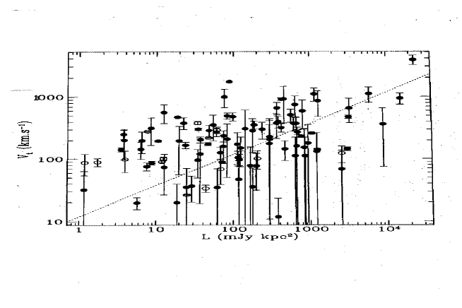
Figure 8: Pulsar Speed vs. Luminoscity

4.1 Pulsar Kicks From Standard Neutrino Emission

The origin of these large velocities, called pulsar kicks, has been a problem for decades. The pulsars are created during supernova explosions:

A massive star ($\geq~{}$ 8 sun masses) burns its nuclear fuel in less than a billion years and undergoes gravitational collapse:

1. Collapse to density $>10^{14}$ g cm${}^{-3}>$ nuclear density

2. Protoneutron star formed $\sim$ 0.01 s.

Neutrinos trapped in neutrinosphere. Radius of neutrinosphere $\sim$ 40 km.

3. From 0.1 to 10 sec neutrinosphere contracts from $\sim$ 40 km to protostar radius $\sim$ 10 km. The URCA process dominates neutrino emission ( $n\rightarrow p+e^{-}\bar{\nu};e^{-}+p\rightarrow n+\nu_{e};e^{+}+n\rightarrow p+\bar{\nu}_{e}$, where the nucleons are polarized by the strong magnetic fields of the protoneutron star. However, since the mean free path of neutrinos is only 1 cm, and the asymmetric neutrinos are not emitted. Therefore standard active neutrinos cannot explain pulsar kicks during the first 10 sec.

4. From $\sim$ 10 to $\sim$ 50 sec n-n collisions dominate neutrino production and protoneutron star cooling. The modified URCA process dominates energy emmision by neutrinos.

$$n+n \rightarrow n+p+e^{-}+\bar{\nu}_{e}$$

It was shown that the modified URCA process during 10-50s might explain pulsar kicks[11]

4.2 Pulsar Kicks From Sterile Neutrino Emission

Just as neutrinos of different flavors mix, as discussed above, active neutrinos can oscillate into sterile neutrinos, neutrinos without an even a weak interaction.

Sterile/active neutrino mixing given by the mixing angle $\theta_{m}$

$$|\nu_{1}> = cos\theta_{m}|\nu_{e}>-sin\theta_{m}|\nu_{s}>$$ (15)

$$|\nu_{2}> = sin\theta_{m}|\nu_{e}>+cos\theta_{m}|\nu_{s}>\;.$$

At the time Ref[13] as published, $\theta_{m}$ was not known well enough for the theory to be compared to measured pulsar velocities, but recently[14] it has been determined to about 30 per cent:

$$sin^{2}(2\theta_{m}) \simeq 0.15\pm.05\;,$$ (16)

and this was used to estimate the pulsar velocities[15].

The neutrino emissivity, $e^{\nu}$=energy/(volume x $\Delta t$), where $\Delta t$ is the time interval for the emission, from Ref[12] is

$$e^{\nu} = \Pi^{4}_{i=1}\int\frac{d^{3}p^{i}}{(2\pi)^{3}}\frac{d^{3}q^{\nu}}{2\omega^{\nu}(2\pi)^{3}}\int\frac{d^{3}q^{e}}{(2\pi)^{3}}$$

$$(2\pi)^{4}\sum_{s_{i},s^{\nu}}\frac{1}{2\omega^{e}_{L}}\omega^{\nu}\mathcal{F}|M|^{2}$$

$$\delta(E_{final}-E_{initial})\delta(\vec{p}_{final}-\vec{p}_{initial})\;,$$

where $M$ is the matrix element for the URCA process and $\mathcal{F}$ is the product of the initial and final Fermi-Dirac functions. The $p^{i}$ are the two initial and two final nucleon momenta, and $q^{\nu},q^{e}$ are the neutrino and electron momenta.

The result for the asymetric neutrino emission along the direction of the magnetic field, which can produce pulsar kicks, is[11]

$$\epsilon^{AS} \simeq 0.64\times 10^{21}T_{9}^{7}P(0)\times f$$ (18)

$${\rm erg\;cm^{-3}\;s^{-1}}=p_{ns}c\frac{1}{V_{eff}\Delta t}\;,$$

where $T_{9}=T/(10^{9}K)$, $p_{ns}$ is the neutron star momentum, $P(0)\simeq$ 0.3 is the probability of the electron produced with the antineutrino being in the lowest Landau state, f=.52 is the probability of the neutrino being at the + z neutrinosphere surface [11], $V_{eff}$ is the volume at the surface of the neutrinosphere from which neutrinos are emitted, and $\Delta t\simeq 10s$ is the time interval for the emission.

Although the sterile neutrino has no interaction, it oscillates back to an electron neutrino as shown in Eq(15). The effective mean free path is abour five times longer than the active neutrinos. $V_{eff}$, the volume at the surface of the neutrinosphere from which neutrinos are emitted, is given by the mean free path of the sterile neutrino, $\lambda_{s}$, and the radius of the neutrinosphere[13]:

$$V_{eff} = (4\pi/3)(R_{\nu}^{3}-(R_{\nu}-\lambda_{s})^{3})$$ (19)

$$\simeq 4\pi R_{\nu}^{2}\lambda/sin^{2}(2\theta_{m})\;,$$

with $\lambda_{s}=\lambda/sin^{2}(2\theta_{m})$, where $\lambda$ is the active neutrino mean free path. Therefore

$$p_{ns} = 4\pi R_{\nu}^{2}(\lambda/sin^{2}(2\theta))(10s)\epsilon^{AS}\;.$$ (20)

Using $p_{ns}=M_{ns}v_{ns}$, with $M_{ns}$the mass of the neutrino star, and taking $M_{ns}=M_{sun}=2\times 10^{33}$ gm, one finds with $sin^{2}(2\theta)$=.15

$$v_{ns} \simeq 22.3\times 10^{-7}(\frac{T}{10^{10}K})^{7}\frac{km}{s}\;.$$ (21)

During the early stages after the collapse of a massive star temperatures T=20 MeV are expected[16]. With T = 10 to 20 MeV the pulsar velosities, with a 50% range due to the uncertainty in $sin^{2}(2\theta)$, are shown in the figure below[15].

Figure 9: The pulsar velocity as a function of T for $sin^{2}(2\theta)=.15\pm.05$

As can be seen in Fig. 9., pulsar velocities of over 1000 km/s are predicted from sterile neutrino emission with the mixing angle recently measured[14]. Therefore, sterile neutrino emission can account for the large pulsar velocities for high luminosities (large T) that have been measured, as shown in Fig. 8. This is a possible explanation of a puzzle that many have tried to explain for decades.

5 Neutrino Energies in a Neutrinosphere

More than a decade ago, in preperation for studies of neutrino oscillations, energy eigenvalues of neutrinos in the earth were investigated by Freund[17] using a cubic eigenvalue formalism.

Recently, this formalism has been used to find the energy eigenvalues of neutrinos in a neutrinosphere[18], through which neutrinos must move to provide the pulsar kicks discussed in the previous section. We define the energy of a neutrino with zero velocity as it’s effective mass, which is the definition of mass in vacuum.

Using the method of Ref [17], the neutrino energy eigenvalues $E_{i}$,

$$H|\nu_{i}> = E_{i}|\nu_{i}>\;,$$

are found as eigenvalues of the matrix $M$[17] obtained from the 3 x 3 matrices $U$ and the Hamiltonian $H$:

$$M=\left(\begin{array}[]{lcr}s_{13}^{2}+\hat{A}+\alpha c_{13}^{2}s_{12}^{2}&\alpha c_{13}s_{12}c_{12}&s_{13}c_{13}-\alpha c_{13}s_{13}s_{12}^{2}\\ \alpha c_{13}s_{12}c_{12}&\alpha c_{12}^{2}&-\alpha s_{13}s_{12}c_{12}\\ s_{13}c_{13}-\alpha c_{13}s_{13}s_{12}^{2}&-\alpha s_{13}s_{12}c_{12}&c_{13}^{2}+\alpha s_{13}^{2}s_{12}^{2}\end{array}\right)$$ (25)

With $c_{ij}\equiv cos(\theta_{ij}),s_{ij}\equiv sin(\theta_{ij})$, and $\delta m_{rs}^{2}\equiv m_{r}^{2}-m_{s}^{2}$, the parameters in M are: $c_{12}^{2}=0.69,c_{13}^{2}\simeq 1.0,\delta m_{12}^{2}=7.59\times 10^{-5}eV^{2},\delta m_{13}^{2}=2.45\times 10^{-3},\alpha\equiv\delta m_{12}^{2}/\delta m_{13}^{2}=0.031,\hat{A}=2E_{\nu}V/\delta m_{13}^{2}$ , with $V$ the potential for neutrino interaction in matter. It is well-known that $V=\sqrt{2}G_{F}n_{e}$, where $G_{F}$ is the weak interaction Fermi constant, and $n_{e}$ is the density of electrons in matter. For neutrinos in earth $V\simeq 1.13\times 10^{-13}eV$, $\hat{A}\ll 1.0$

The eigenvalues of M satisfy the cubic equation (see Eq(17) in Ref[17] with a=$-I_{1},b=I_{2},c=-I_{3}$):

$$\bar{E}_{i}^{3}+a\bar{E}_{i}^{2}+b\bar{E}_{i}+c = 0$$ (26)

$$a = -(1+\hat{A}+\alpha)$$

$$b = \alpha+\hat{A}\alpha c_{12}^{2}c_{13}^{2}+\hat{A}(c_{13}^{2}+\alpha s_{13}^{2})$$

$$c = -\hat{A}\alpha c_{12}^{2}c_{13}^{2}\;$$

with dimensionless quantities $\bar{E}_{i}=(E_{i}-E^{0}_{1})/(E^{0}_{3}-E^{0}_{1})$, where $E_{i}^{0}$ are neutrino energy eigenvalues with V=0. We study neutrinos at rest, so $E_{i}\equiv m_{i}c^{2}\equiv m_{i}$, with i = 1, 2, and 3; $E^{0}_{i}$ are the neutrino masses in vacuum, and $m_{i}$ are the effective masses of neutrinos in matter. With the parameters given abovone finds,

$$a = -(1.031+\hat{A})$$

$$b = 0.031+\hat{A}$$

$$c = -0.0209\hat{A}\;.$$ (27)

Taking $E_{\nu}\simeq m_{3}\simeq\sqrt{\delta m_{13}^{2}}$, as $m_{1}\ll m_{3}$, for which $\hat{A}$ is maximum, results in the largest matter effect on neutrino eigenstates. First, we solve the cubic equations for neutrinos in vacuum. From Eqs.(26,5) for V=0 ($\hat{A}=0$)

$$\bar{E}_{1} = 3.08\times 10^{-12}\simeq 0$$

$$\bar{E}_{2} = 0.031$$

$$\bar{E}_{3} = 1.0\;,$$ (28)

which is nearly the same as for neutrinos in earth ($\hat{A}\ll 1.0$).

The density of nucleons in the neutrinosphere is approximately that of atomic nuclear matter, $\rho_{n}=4\times 10^{17}kgm/m^{3}$. Taking the ratio of the electron mass to the proton mass one finds for the electron density in the neutrinosphere $\rho_{e}\simeq 2\times 10^{11}$ gm/cc, giving the neutrino potential in the neutrinosphere $V\simeq 10^{-2}$ eV. . This gives $\hat{A}_{ns}=0.404$, which is $\hat{A}$ for neutrinos in a neutrinosphere. Solving Eq(26) with this dense matter potential one finds

$$\bar{E}_{1}^{ns} = 0.0208$$

$$\bar{E}_{2}^{ns} = 0.3998$$

$$\bar{E}_{3}^{ns} = 1.0144\;,$$ (29)

Comparing Eq(5) with Eq (5), $m_{3}\simeq m_{3}(V=0)$, while $m_{2}-m_{1}(V=0)\simeq 0.4eV\simeq 13.0\times(m_{2}(V=0)-m_{1}(V=0))$. Therefore, the neutrino effective masses in the neutrinosphere are quite different than in earth or vacuum. Although the three neutrino effective masses are approximately the same in earth matter as in vacuum, the large effect of matter on neutrino oscillations arise from a large baseline and depend on the energy of the neutrino beam.

6 Conclusions

1) Although neutrino oscillations are promising for determining TRV and CPV, new experimental facilities are needed.

2) Neutrino oscillation, such as neutrino disappearance, can provide accurate measurements of the parameters in U, the matrix relating flavor neutrinos to mass neutrinos.

3) Sterile neutrino emission during the first 10 seconds after the gravitational collapse of a star can explain the large pulsar velocities.

4) The effective masses of neutrino in a neutrinosphere are very different than those in earth of vacuum

Acknowledgements

The author thanks Drs. M.B. Johnson and E.M. Henley for helpful discussions. This work was supported in part by a grant from the Pittsburgh Foundation.

References

- [1] E. Akhmedov, P. Huber, M. Lindner, and T. Ohlsson, Nucl. Phys. B608, 394 (2001)
- [2] M. Jacobson and T. Ohlsson, Phys. Rev D 69, 013003 (2004)
- [3] E.M. Henley, M.B. Johnson, and L.S. Kisslinger, Int. J. Mod. Phys. E 20, 2463 (2011)
- [4] M. Freund, Phys. Rev. D64, 053003 (2001)
- [5] L.S. Kisslinger, E.M. Henley, M.B. Johnson, IJMPE, Vol 21, 12920 (2012))
- [6] J.H. Christenson, J.W. Cronin, V.L. Fitch, and R. Turlay, Phys. Rev. Lett. 13, 138 (1964)
- [7] J.W. Cronin, P.F. Kunz, W.S. Risk, and P.C. Wheeler, Phys. Rev. Lett. 18, 25 (1967)
- [8] L.S. Littenberg, Phys. Rev. D 39, 3322 (1989)
- [9] L.S Kisslinger, Int. J. of Mod. Phys. E 21, 1250065 (2012)
- [10] L.S. Kisslinger, E.M. Henley, M.B. Johnson, IJMPE-D-12, 0053R2 (2012)
- [11] E.M. Henley, M.B. Johnson, and L.S. Kisslinger, Phys. Rev D 76, 125007 (2007)
- [12] B.L. Friman and O.V. Maxwell, ApJ 232, 541 (1979)
- [13] E.M. Henley, M.B. Johnson, and L.S. Kisslinger, Mod. Phys. Lett. A24,2507 (2009)
- [14] K. N. Abazajian et al, arXiv:1204.5379 (2012)
- [15] L.S Kisslinger and M.B. Johnson, Mod. Phys. Lett. A27, 1250215 (2012)
- [16] G. M. Fuller, A. Kusenko, I. Mocioiu and S. Pascoli, Phys. Rev. D 68, 103002 (2003)
- [17] M. Freund, Phys. Rev. D64, 053003 (2001)
- [18] L.S. Kisslinger, arXiv:1211.3348, MPLA-D-13-00011 (2013)