Partial Decoherence and Thermalization through Time-Domain Ergodicity

Abstract

An approach, differing from two commonly used methods (the stochastic Schrödinger equation and the master equation [2, 3]) but entrenched in the traditional density matrix formalism, is developed in a semi-classical setting, so as to go from the solutions of the time dependent Schrödinger equation  to decohering and thermalized states. This is achieved by utilizing the time-ergodicity, rather than the sampling- (or ensemble-) ergodicity, of physical systems.

We introduce the formalism through a study of the Rabi model (a two level system coupled to an oscillator) and show that our semi-classical version exhibits, both qualitatively and quantitatively, many features of state truncation and equilibration [4]. We then study the time evolution of two qubits in interaction with a bosonic environment, such that the energy scale of one qubit is much larger, and that of the other much smaller than the environment’s energy scale. The small energy qubit decoheres to a mixture, while the high energy qubit is protected through the adiabatic theorem. However, an inter-qubit coupling generates an overall decoherence and leads for some values of the coupling to long term revivals in the state occupations.

1 Introduction

Safe and reliable manipulation of quantum states (as is envisaged in a quantum computer) depends on the possibility of error-free and stable quantum systems when left alone, except for the inevitable interaction with the environment. The devil is in decoherence and numerous works have been devoted to estimate, minimize, circumvent it or to correct for it [2]. Distinct from the direct approaches to provide somehow remedies for decoherence , several avenues have been explored in which the quantum system maintains coherence due to the Hamiltonian the defines it. One of the earliest works related to the subject is by Kubo [6], in which hints for the approach taken in the present paper can be found. While decoherence and dissipation are terms very close to each other, ”dissipationless decoherence” was also considered [7] and decoherence-free subspaces in the Hilbert- space were studied in [8]. In more recent works such subspaces were identified, manifesting ”partial decoherence”, through symmetry-based discrimination between parts of the Hilbert-space [9]-[10].

The present work also treats partial decoherence, but differs from the previous in that, rather than throwing the burden of discrimination on a specially contrived Hamiltonian, it finds discrimination between Hilbert subspaces more generically, through their having different energy scales. A simple physical example of this is an atomic system in the presence of a magnetic field of 1 tesla, for which the electronic spins separate to about 10 cm^-1 and the nuclear spins to about 10^-2 cm^-1. As already indicated, an allied idea was briefly noted by Kubo [6], who differentiated between the cases of fast and slowly modulated frequencies of the relaxing system. A further idea borrowed in the present work from that paper (and indeed from other treatments involving ”ergodicities”) is equating ensemble averages with long time averages [5].

The proposed semi-classical formalism (which is the main novelty of this work) is introduced and tested in section 2 on the single qubit(or $\frac{1}{2}$ spin)-single boson (Rabi) model [11]. This was thoroughly treated algebraically [12]-[16] and applicatively: for single trapped ions [17], chiral molecules in a three-level system [18], Josephson junctions [19], a single photon coupled to to a superconducting (SC) qubit [20], the Bloch-Siegert shift in a SC flux qubit[21]; all these somewhat with a long term view of decoherence-ridden quantum computing. The case of two qubits, in interaction with a single classical oscillator and having largely differing Zeeman splitting energies, is considered in section 3 and is the essential motivation for this work. The two qubit case featured in [22] and was recently treated algebraically in [23] in cases amenable to adiabatic treatment, but when the two qubits have identical splitting energies.

2 Decoherence in a Semi-classical Rabi model

Here the spin-vibration Hamiltonian

$$H(t,a)=e\sigma_{z}+k\sigma_{x}\sin(\omega t+\alpha_{a})~{}~{}~{}(\omega\to 1)$$ (1)

describes our two-parameter system, involving a Zeeman-split 1/2-spin [represented by the Pauli matrices $\sigma_{z}=\left(\begin{array}[]{cc}1&0\\ 0&-1\end{array}\right)$, $\sigma_{x}=\left(\begin{array}[]{cc}0&1\\ 1&0\end{array}\right)$] and a classical vibrator, whose frequency $\omega$ is equated to 1, thus setting the time (t) scale and the energy scales of the splitting $2e$ and of the spin-vibration coupling $k$. $\alpha_{a}$ is an initial phase of the classical vibrator, whose value is specified by the indexing parameter $a$. The Hamiltonian of the classical vibration is not needed. In our procedure the time dependent Schrodinger equation (TDSE) [$i\frac{d\psi_{a}(t)}{dt}=H(t,a)\psi_{a}(t)]$ is solved numerically with some fixed initial conditions.

2.1 Programmatic summary of the three steps to construct the density matrix $\rho_{mn}$

1. We adopt the von Neumann definition [24]-[26]:

   $$\rho_{mn}(t)=\frac{1}{(\sum_{a}1)}\sum_{a}<m|\psi_{a}(t)><\psi_{a}(t)|n>$$ (2)

   In this definition the summation index $a$ represents the values of all coordinates, variables etc. external to the system (e.g., those of the environment affecting the system) and appearing also in the Hamiltonian. Thus the set ${\psi_{a}(t)}$ for all $a$’s forms a time dependent ensemble of states. The degrees of freedom of the system themselves are implicit (not written out) in $\psi_{a}(t)$.

2. We solve only for a single external condition thus dispensing with the $a$ index in the wave function, but obtain $\rho(t)$ as the average over an adequate set of adjacent times:

   $$\rho_{mn}(t)=\frac{1}{2\Delta t}\int_{t-\Delta t}^{t+\Delta t}d\tau<m|\psi(\tau)><\psi(\tau)|n>$$ (3)

   This should be equivalent to equation (2) if the ergodic hypothesis holds for the duration $2\Delta t$. (It also represents a considerable simplification in numerics, since the TDSE is only solved once, specifically for $\alpha=0$. To justify the replacement of step 1 by step 2 we note that in all cases considered, numerically computed non diagonal density matrix elements were several orders of magnitude smaller than the diagonal ones. Thus decoherence, which is the ”truncation” of [4], was achieved. The time-averaging method also avoids the notorious ”initial slippage” problem [27]. More detailed motivation for step 2 is given in the Discussion section, after the reader has become informed of the proposed method).

3. For the basis $n,m$ set we have chosen two alternative representations: (a) the spin eigenstates, up: $\left(\begin{array}[]{c}1\\ 0\end{array}\right)$ and down:$\left(\begin{array}[]{c}0\\ 1\end{array}\right)$, and (b) the time dependent adiabatic representation, which is given by the two instantaneous solutions $u(t)$ of $H(t,a)u(t)=w(t)u(t)$ with $w(t)$ the adiabatic energies. While the spin up/down representation has featured in many works (e.g., [12]-[16]), the broader issue of representation choice in the density matrix has been intensively studied, e.g. in terms of the ”einselection” in quantum measurements [28] and for the preference of energy states [29].

Further discussions of these steps are given in the sequel.

2.2 The significance of averaging in steps 1 and 2

Clearly, without an averaging the density matrices could be brought to a pure state form, with only one (diagonal) element unity and all the rest being zero. Illustrating this for an $N$ x $N$ density matrix when $N=2$, one can write the density matrix in the alternative forms

$$\left(\begin{array}[]{cc}a^{*}\cdot a&a^{*}\cdot b\\ b^{*}\cdot a&b^{*}\cdot b\end{array}\right)\equiv\begin{array}[]{c}a^{*}\cdot\\ b^{*}\cdot\end{array}\left(\begin{array}[]{cc}a&b\\ a&b\end{array}\right)$$ (4)

showing that the two rows are linearly related. Therefore one eigenvalue of the matrix is zero, while the other eigenvalue is, by invariance of the trace,

$$a^{*}\cdot a+b^{*}\cdot b=1$$ (5)

due to normalization. The density matrix can thus be brought to a form for a pure state. The same procedure holds also for any density matrix of size $N$ x $N$, with $N>2$, where the number of linear relations, and therefore of zero eigen-values is $N-1$. It is only when an averaging is performed first and the diagonalization of the averages is made subsequently, that a mixed state can arise and decoherence, with the vanishing of off-diagonal density matrix elements, emerges.

However, to proceed literally as described in step 1, namely summing the density matrix over all (in practice, say, 1000) initial phases of the oscillators would have meant to solve the TDSE 1000 times and to save all these solutions. Instead, as noted in step 2 above, we have solved it only once for one parameter set and averaged all density matrix elements over some time interval $2\Delta t$. This time interval will be specified as we progress, the criterion being that an averaging over a greater interval does not alter the value of the averages. The relation of this procedure to an ensemble averaging is rooted in the ergodic theorem (or hypothesis) [5]. We have also constantly checked our results for error and found that the full trace of the averaged density matrix deviated from (was short of) unity by less than $4\%$, though we have extended our computations over about 200 times the vibrational period ($2\pi/\omega$). Moreover, the normalization check of the wave propagated wave function was also in error by the same margin (about $4\%$), indicating that the error in the density matrix has arisen from numerical errors in the forward integration and not from inadequate tracing (averaging).

2.3 The ”environment interaction”

A widespread formulation of the interaction of a bosonic environment with a spin system is to write the interaction of the spins with one or more oscillators in the form

$$\sum_{n}\sum_{i=x,y,z}k^{i}_{n}q_{n}\sigma_{i}$$ (6)

where $q_{n}$ is the $n$-th oscillator’s amplitude and $k^{i}_{n}$ its coupling strength for the interaction with the spin [30, 31]. The behavior of the closed (spin-boson) system is studied through its density matrix $\rho_{s,b}$. The reduced density matrix of the spin system $\rho_{s}$ is then obtained from the trace $Tr_{b}\rho_{s,b}$ over all boson states and modes of the environment.

What is the relation of this formulation to our model?

In equation (1) we have chosen an (Einstein-) model for the oscillators, so that their frequencies are the same (denoted by $\omega$ and equated to $1$). However, the stochastic (random) effect of the environment on the spin systems is still present through each oscillator having a different phase $\alpha_{a}$, randomly distributed between $0$ and $2\pi$. We then replace the ${\it set}$ of randomly phased oscillators acting together by an ${\it ensemble}$ of independently acting oscillators, each oscillator having a phase $\alpha_{a}$, randomly distributed over the ensemble states. Here $a$ enumerates members of the ensemble. In summary, by the adopted semi-classical approximation for our model in equation (1) , the oscillator amplitudes and coupling strengths in equation (6) take the (unnormalized) forms

$$q_{a}=\sin(\omega_{a}t+\alpha_{a}),~{}k^{x}=k,k^{y}=k^{z}=0$$ (7)

with $a$ labelling different states of the environment. In the von Neumann averaging in equation (2), it is the values of $\alpha_{a}$ that are to be summed over (eventually, integrated) .

In the sense of spin-environment perturbation, the sine term represents highly colored noise.

In the next development of the present formalism, noted in the previous subsection and in step 2 of section 2.1, the averaging over the solutions with differing initial phases $\alpha_{a}$ has been replaced by averaging over a time interval $2\Delta t$.

2.4 Decoherence Results

The decohered diagonal matrix elements with time averaging over about five vibration periods and after reaching equilibration (such that longer times do not essentially change the average values and with near zero off-diagonal matrix elements, not shown) are presented in Figures 1-4, (a) in the spin representation (broken line) and (b) in the adiabatic, time-instantaneous state representation (dotted line). In figure 1 for weak spin-oscillator coupling ($k<<1$) the initial (upper) state’s density matrix (mean occupation probability) is close to one, but then decays to $\frac{1}{2}$ as the coupling $(k)$ increases. The computed lower state’s mean occupation probability was found to be (1 minus the one shown), correct to about 0.001, verifying the normalization of the density matrix. The limiting value of $\frac{1}{2}$ is appropriate to equilibration with an oscillator bath at infinite temperature, which pertains to this model. (Finite temperatures and thermalization are treated in the next section.).

There are sudden jumps, here as in the following figures, whose nature is not clear, but probably reflect some resonances (i.e., occurrences when the instantaneous energy differences between the states match the oscillator frequency, $\omega=1$). To discount the time-windows as the sources for the peaks (and also to provide assurances for the reliability of the time averaging procedure), we have consistently checked the accuracy of the averages, by varying the time-window by 60-100 percents. The variations caused changes in the time averages that were comparable to widths of the line in our figures. Sharp variations in the state probabilities were also seen for relatively small variations in the parameters of the Hamiltonian in figure 9 of [12] (there termed ”unusual behavior”).

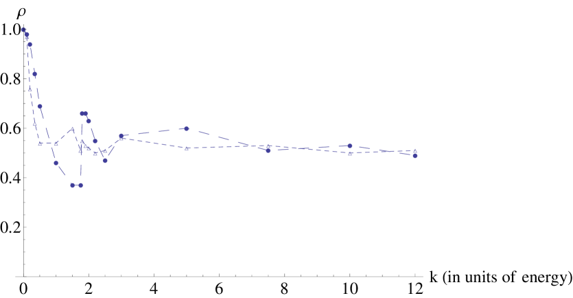
Figure 1: Decohered density matrix elements as functions of the spin-classical oscillator coupling $k$ for small spin energy $e=0.1$. Dots (connected for visual convenience by long broken lines): Spin up probability. Triangles (connected by short broken lines): Upper energy state occupation in the adiabatic energy state representation.

In figure 2 the same quantities are shown for spin energy $e=1$, of the same value as the oscillation frequency. The equilibration starts for larger $k$ and the oscillations (resonances?) are stronger.

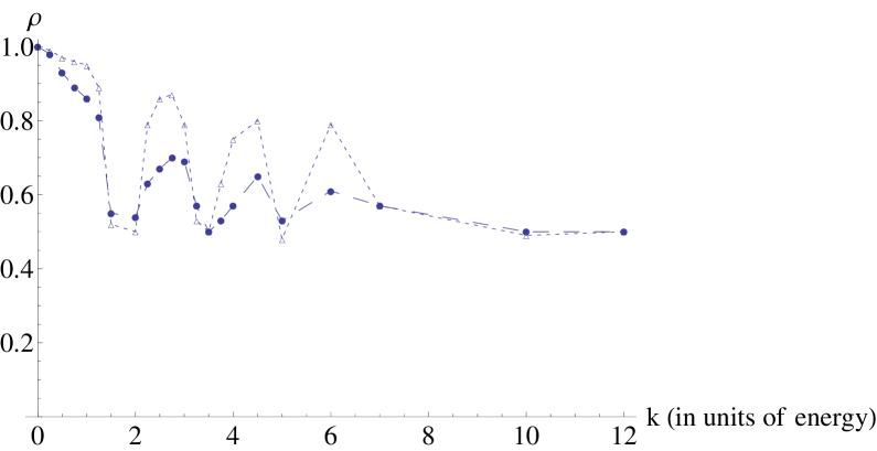
Figure 2: Decohered density matrix elements as functions of coupling strength $k$ for moderate spin energy $e=1$. Dots: Spin up probability. Triangles: Upper energy state occupation in the adiabatic energy state representation.

The third drawing, figure 3 is for spin energy $e=10>>1=$ (the vibration frequency $\omega$), representing a situation, where the adiabatic theorem holds, so that there is no environment induced mixing of states. As seen, this holds for moderate values of the coupling, but for very strong coupling ($k>>1)$ the adiabaticity-protection breaks down.

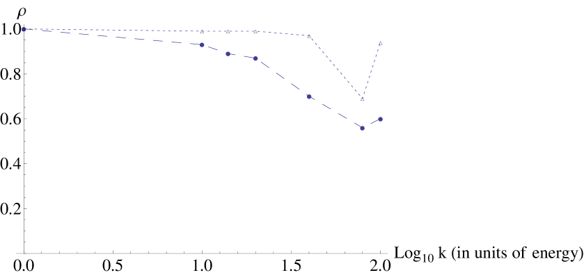
Figure 3: Decohered density matrix $\it vs$ $k$ in the adiabatically protected spin (e=10) regime. Meaning of curves as before. The coupling parameter $k$ reaches up in this figure only to $2$, for much larger values the numerical results were not reliable.

Figure 4 shows the inverse situation that the coupling strength is held fixed at $k=2.5$ and the spin energy is varied from $e\simeq 0$ (equilibrated case) to a large value (the adiabatically protected regime).

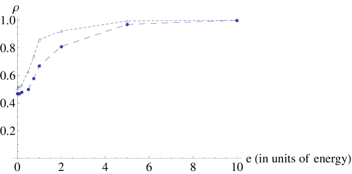
Figure 4: Decohered density matrix plotted against spin energy $e$ for fixed coupling strength $(k=2.5)$. Curve description, as before.

2.5 Thermalization

While the former results in figures 1-4 showed decoherence at essentially infinite temperature ($T\equiv 1/(k_{B}\beta)~{}->\infty$), or with the same probability for up and down flipping by the oscillator, at finite temperatures the two probabilities differ. Since in our model stochasticity enters through time-averaging, we include temperature effects by weighting the time duration according to the energy of the system, meaning that excursions at lower energies have greater time-weights than those at higher energies. Quantitatively, we express equation (3) in the adiabatic energy representation, in which $m(t)$ indexes the two states in the adiabatic representation. Then replace the diagonal terms in equation (3) by:

$$\rho_{mm}(t)=\frac{1}{2\Delta t}\int_{t-\Delta t}^{t+\Delta t}d\tau\frac{e^{-\beta E_{m}(\tau)}|<m(\tau)|\psi(\tau)>|^{2}}{<\psi(\tau)|e^{-\beta H(\tau)}|\psi(\tau)>}$$ (8)

in which the denominator in the integrand ensures the normalization of the density matrix. The off-diagonal elements are negligible also in the thermalized density matrix.

An intuitive justification for the chosen time-weighting can be based on the early work Rechtman and Penrose [32], who have shown that the probability distribution for a finite classical system, in thermal contact with an infinite (in practice, sufficiently large) heat bath, with the composite system being distributed micro-canonically, is the Gibbs canonical distribution $e^{-\beta E}$, where $E$ is the energy of the system. This has the meaning that for a state of energy $E$ of the system and no degeneracies, the number of micro-states of the heat-bath is proportional to $e^{-\beta E}$. If we now suppose that the heat bath spends equal time in each micro-state (cf. the ergodic hypothesis), then in the system’s time integration the infinitesimal $dt$ has to be weighted by the Gibbs factor, as in equation (8) .

To check the validity of our proposed thermalization procedure, we investigate whether we regain through it the ”$\rho_{mm}=e^{-\frac{E_{m}}{k_{B}T}}/Z$” law? In figure 5 we show the logarithm of the ratio of the up and down (time-averaged) diagonal density matrices in the adiabatic state representation, divided by the adiabatic energy difference, against the inverse temperature $\beta\equiv\frac{1}{k_{B}T}$. In thermalized energy eigenstates the plot should be linear in $\beta$ with a slope of one. This is approximately the case for the three lower curves (in which $k\leq 1$, weak to moderate spin-oscillator coupling), but for the uppermost curve (in which $k=2.5$) the spin is too much interwoven with the environment to thermalize independently of it.

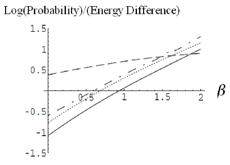
Figure 5: Thermalized density of states. The input parameters for the curves from bottom to top (at $\beta=0$ or infinite temperature) are the following: Solid line: spin energy $e=0.5$, coupling $k=1$, time*frequency = 270, vertical displacement = 0, (in this curve the mean slope is 1). Dotted line: $e=0.5$, $k=1$, time*fr. = 60, vertical displacement = 0.2. Chained line: $e=5$ (near adiabatic), $k=0.2$, time*fr. = 250, vertical displacement = 0.6. Long broken line: $e=0.1$, $k=2.5$, time*fr. = 250, vertical displacement = 0.4. Curves are displaced vertically for visual clarity.

2.6 Revivals

To establish the compatibility of our approach with previous works (some of them analytic) on the Rabi model, we turn to a study in which the oscillator state was modelled by a coherent state ([12], section III). As is well known, coherent quantum states resemble closely the behavior of a classical oscillator (which features in our Hamiltonian). Long period (compared to the oscillator’s period) revivals in the up (or down) spin-state probabilities (equivalent to the diagonal terms in the reduced density matrix) were shown in Figure 7(a) of that paper in the adiabatic limit. The curve computed by us and shown in Figure 6 (persistent for many further periods, not shown) is extremely similar to their result for a coherent state. Our parameter choice ($e$, spin energy $=.05$, $k$, spin-oscillator coupling strength $=2.5$) is not immediately translatable to that ($<N>=1,\lambda/\omega=0.1$) in [12], since the coupling strength $k$ in our semi-classical formalism is a combination of these. We have also found that the complete revival pattern shown in Figure 6 occurs for only a restricted choice of parameters and is not a universal feature of the model. However, referring to the drawings (a) to (e) in figure 9 of [12], we note that also in their model even slight changes of the parameters cause radical changes in the patterns.

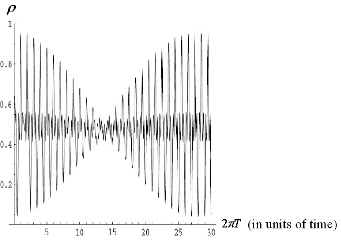
Figure 6: Time-averaged spin-up probability. Model parameters: $e$, spin energy $=.05$, $k$ (the spin-oscillator coupling strength) $=2.5$, time averaging over $1.2/\omega$, $\omega=1$.

3 Two Qubit Systems

The following Hamiltonian $\textbf{H}_{total}(t)$ involves two half-spin systems (qubits), whose parameters are in the sequel consistently designated by capital and lower-case letters, respectively, interacting with a classical boson source (as before, vibrational or light-like) varying with time.

$$\textbf{H}_{total}(t) = H(t)+h(t)+\textbf{H}_{int}$$ (9)

$$H(t) = E\Sigma_{z}+K\Sigma_{x}\sin(\omega t+\alpha)$$ (10)

$$h(t) = e\sigma_{z}+k\sigma_{x}\sin(\omega t+\alpha^{\prime})$$ (11)

$$\textbf{H}_{int} = \gamma(\Sigma_{z}\cdot\sigma_{z}+\Sigma_{x}\cdot\sigma_{x})+\gamma^{\prime}(\Sigma_{x}\cdot\sigma_{x}+\Sigma_{y}\cdot\sigma_{y})$$ (12)

having written in the first line the total Hamiltonian, comprising, as in the following lines, the Hamiltonians of the large- and the small-symbol system, ending with the interaction between these. In them $E,e$ are energies of the two spin systems, the $\Sigma$’s (!) and $\sigma$’s are Pauli matrices operating in the respective spin-spaces, $K,k,\alpha$, are parameters of the spin-boson couplings and $\omega$ is the frequency of the interacting source. The external boson source is classical and for it the Hamiltonian need not be written out.

The strengths of the Spin-spin interaction are denoted by $\gamma$ and $\gamma^{\prime}$. For the form of the interaction two alternative sub-models will be used: The first, named ”The two-dimensional model”, for which $\gamma\neq 0$ and $\gamma^{\prime}=0$, is fashioned after the $E\bigotimes e$ vibronic interaction [33]. The second, in which $\gamma^{\prime}\neq 0$ and $\gamma=0$, commonly features in Ising models and is known as the ”transverse interaction”. It has been recently used for superconductors with a large pseudo-gap and weak long rage Coulomb interaction [34].

The double inequality (exemplified with a physical model in the Introduction):

$$E>>\hbar\omega>>e$$ (13)

is the keynote to the present section, in that it makes the time variation in the Hamiltonian slow (adiabatic) with respect to that of one of the spins (the ”capitalized” one) and fast (non-adiabatic) with respect to that of the other (”the lower-case” one). It is therefore expected that the distilled wave function in the former’s Hilbert space will stay coherent, while that one in the latter’s Hilbert space will decohere. This result is indeed found, with some interesting features to be expatiated on in the sequel. (Two spin systems with identical energies were treated in the adiabatic limit in [23].)

We wish to investigate decoherence in the combined system. In an overwhelmingly large number of papers ”Decoherence”, leading from an initially pure to a later mixed state, has been obtained by going from the density of states in the full to a partial Hilbert space, through tracing over the complementary Hilbert space (e.g, references in [4]). As noted earlier in the programmatic summary of section 2.1, we use an alternative procedure for decoherence, namely an external parameter averaging procedure. In terms of our model, in which the environment is represented by a classical oscillator, this means that after obtaining a (time-dependent) solution $\psi_{\alpha,\alpha^{\prime}}(t)$ for given phases $\alpha,\alpha^{\prime}$, we average the elements of the density matrix $\rho_{nm}(t)$, with respect to all values of these parameters. Then, formallly

$$\rho_{nm}(t)=(4\pi^{2})^{-1}\int_{0}^{2\pi}d\alpha\int_{0}^{2\pi}d\alpha^{\prime}<n|\psi_{\alpha,\alpha^{\prime}}(t)><\psi_{\alpha,\alpha^{\prime}}(t)|m>$$ (14)

for some chosen representation, whose components are labelled $(n,m)$. This procedure differs from the commonly used ones (e.g., the stochastic Schrödinger equation or a time-propagation equation for the reduced density matrix) in which the environment is also in a quantum state, whose nature is specified by its spectral properties [37]. Still the method used here is historically primordial (coming from [24, 25]). It is also suitable for numerical calculations and alleviates to some extent the classical-quantal dichotomy, extensively treated in [4].

The four component wave function $\psi$ is inserted from the numerical solution of the time dependent Schrödinger equation (with $\hbar=1$)

$$i\frac{\partial\psi_{\alpha,\alpha^{\prime}}(t)}{\partial t}=\textbf{H}_{total}(t)\psi_{\alpha,\alpha^{\prime}}(t)$$ (15)

with the appropriate initial condition at $t=0$. This system is then in a pure state; to track down its progression in interaction with a stochastic environment towards a (possibly) mixed state, we need to consider the density matrix of the system.

As already remarked, the density matrix is representation dependent (though its trace is not), and the choice of the representation (labelled above $nm$) for the density matrix was extensively discussed in several publications, e.g. [28]. The conclusion there was that an ”environment induced selection (einselection)” takes place due to the (experimentalist’s) choice of the pointer, which is expressed by the form of the interaction between the environment and the system. In this choice, the off-diagonal matrix elements of the system’s density matrix vanish in a time shorter than other time scales in the system’s Hamiltonian. (It will be seen that our numerical results support their choice for ”einselection”.) Furthermore, under conditions of weak coupling and large energy scales it was formally shown in [29] that the choice pointer states are the discrete energy states of the system. In this context, one recalls an early, somewhat enigmatic statement in [35]: ”In general, only quantities quasi-diagonal in the energy representation are observable”.

This has dictated the choice for one of our two adopted representations (”b” in the programmatic summary in section 2.1) as the adiabatic solutions of the Hamiltonian, namely the instantaneous (upper and lower energy) solutions $u(t),l(t)$ for the small-energy part of the Hamiltonian [36], i.e.,

$$h(t)[u(t)/l(t)]=w_{u/l}(t)[u(t)/l(t)]$$ (16)

and likewise the adiabatic solutions $U(t)$,$L(t)$ for the large- energy part of the Hamiltonian:

$$H(t)[U(t)/L(t)]=W_{U/L}(t)[U(t)/L(t)]$$ (17)

Thus the $4$ x $4$ density matrix is written in the representation of $Uu,Ul,Lu,Ll$ in the given order.The appropriate initial condition is an energy eigenstate at $t=0$. The alternative choice for the representation, namely the more conventional spin up/down representation (”a” in section 2.1), is not treated in this, two-qubit section, since we could not find results in the literature to which we might make comparison..

Actually (as already indicated in section 2.1), for the sake of simplifications in our procedure to obtain the density matrix at any time $t$, we have averaged not over the initial parameters $\alpha,\alpha^{\prime}$, but rather, with fixed values of these $\alpha=0=\alpha^{\prime}$, over a spread of the times ($t-\Delta t,t+\Delta t$), $\Delta t$ being in the two-qubit case close to the oscillator period-squared $(2\pi/\omega)^{2}$, or about $40$ in our time units ($\omega=1$) (see integral in equation (14)).

3.1 Non-interacting spin systems

As a start, we consider the simplified situation in which the spin systems do not interact, i.e., that $\gamma=\gamma^{\prime}=0$ in equation (12). Although this case can be treated for the two spins separately, for the sake of continuity with the interacting spin case in later sections, we treat the two spins as belonging to a larger, combined Hilbert space. We show below the resulting $4$ x $4$ density matrix obtained, as described above, from averaging over neighboring times (by an integration over about 10 oscillator periods) and then further representing the obtained averages by their mean values over the full computed time range (in practice: about 500 vibrational periods), together with specification of the standard deviation of the values inside this time range. Obtained results are shown in Figure 7 for the chosen parameter values of

$$E=5,e=0.1,K=2,k=0.125,\alpha=\alpha^{\prime}=0,\gamma=\gamma^{\prime}=0$$ (18)

in units of $\omega$ and they are characteristic of other parameter values.

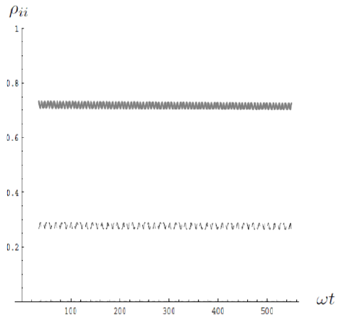
Figure 7: Diagonal density matrix elements $\rho_{ii}~{}(i=[Uu,Ul,Lu,Ll])$ vs normalized time. Time averages of overlap squares are shown in the adiabatic representation described in the text. Only the diagonal matrix elements for $i=Uu,Ul$ (shown in this order from above to below) are visible, while those for $i=Lu,Ll$ are too small to be visible without magnification. Since at any reduced time $\omega t$ the averaging spreads over $\pm 30$, the first shown value is above 30, thus missing the starting values for the four component wave-function (1,0,0,0). The constancy of the averages and the small deviations from these throughout the time range are to be noted.

The time averaged density matrix is shown next:

$$<\rho>=\begin{array}[]{c}<Uu|:\\ <Ul|:\\ <Lu|:\\ <Ll|:\end{array}\left(\begin{array}[]{cccc}0.721\pm.015&10^{-2}&10^{-4}&10^{-4}\\ 10^{-2}&0.272\pm.010&10^{-5}&10^{-3}\\ 10^{-4}&10^{-5}&2\cdot 10^{-4}&10^{-6}\\ 10^{-4}&10^{-3}&10^{-6}&4\cdot 10^{-4}\end{array}\right)$$ (19)

The $\pm$ deviations represent estimated variations in the values over the whole time investigation range. Their signature in Figure 7 are the small wiggles on the otherwise horizontal lines. The off-diagonal entries show upper limits to absolute values. The deviations are partly due to computational inaccuracies, partly to the finite range of the averaging process and partly to the parameters not being in the extreme adiabatic limit.

[It may be added that the above error-checking refers exclusively to the diagonal terms in the density matrix, whereas the averaged off-diagonal matrix elements were unexceptionally negligible. This means that the (adiabatic, instantaneous) representation used here was indeed the proper (”einselected”) one. These results then lend numerical support for the analytical arguments of Paz and Zurek[29].]

3.1.1 Reduced density matrices

With the complementary subsystem traced over, the reduced density matrices for the small and large energy systems are (with suppression of errors), respectively :

$$<\rho_{u/l}>\approx\begin{array}[]{c}<u|:\\ <l|:\end{array}\left(\begin{array}[]{cc}0.721&0\\ 0&0.272\end{array}\right)$$ (20)

$$<\rho_{U/L}>\approx\begin{array}[]{c}<U|:\\ <L|:\end{array}\left(\begin{array}[]{cc}0.993&0\\ 0&0\end{array}\right)$$ (21)

The small energy system is thus seen to have decohered, or be in a mixture state (with the partitioning of the weights depending on the values of the parameters, $e,\omega,k$); while the large energy state is throughout in a coherent, pure state, due to its protectedness by the adiabatic theorem. For situations not belonging to the extreme adiabatic limit (represented by $\frac{E}{\hbar\omega}\longrightarrow\infty$), there will be a finite decoherence time, in the course of which the pure state also decoheres (equilibrates). This decoherence time will decrease as the above ratio decreases, but in our computation range (typically 500 vibrational periods) we have not found for the high-energy (adiabatically protected) states a finite decoherence time.

When the environment coupling to the small energy system was enlarged to $k=0.5$ (instead of $k=0.125$, in the previous case), the diagonal matrix elements took the mean values, with their standard deviation not noted, $[0.804,0.192,.0004,.0000]$

3.2 Systems with Spin-spin interaction

3.2.1 Two-dimensional sub-model,$\gamma\neq 0,\gamma^{\prime}=0$

Weak interaction:

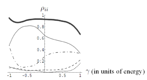
Figure 8: Diagonal density matrix elements $\rho_{ii},i=[Uu,Ul,Lu,Ll]$ (for the thin curves in this order from top to bottom) as function of a weak $\gamma$ (the 2D Spin-spin coupling strength). The strongly drawn curve is the sum of $Uu$ and $Ul$, giving the diagonal U term in the reduced density matrix.

We first investigate how does the interaction between the spin systems modify the decoherence discrimination between adiabatic and non-adiabatic systems. In Figure 8 the diagonal density matrix elements are shown for $|\gamma|\leq 1$. Let us set, somewhat arbitrarily the criterion for decoherence discrimination between large and small energy states as a $80\%$ purity for the large energy states. The thick line in Figure 8 shows the sum of the two uppermost thin curves (for $Uu$ and $Ul$) in that figure: One sees that the $>0.8$ criteria for purity is well satisfied for negative couplings in the range $0>\gamma>-1$, but does not hold near the upper values in the positive range $0<\gamma<1$, for which the two curves do not add up to $0.8$. One also notices that for $|\gamma|\approx 1$ the small energy states ($u$ and $l$) are ”fully” mixed, i.e. their diagonal values are equal. However, this does not hold for higher coupling strength, as Figure 9 illustrates.

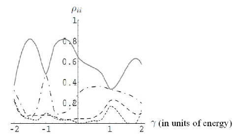
Figure 9: Diagonal density matrix elements against $\gamma$, the 2D Spin-spin coupling strength for extended values of the coupling. Meaning of curves as in previous figure.

Higher interaction strengths:

In Figure 9 one sees that as the coupling strength $\gamma$ is varied a high level of weight exchange takes place between the terms, especially between the diagonal $Uu$ and $Lu$ terms. One notes signs of the ”level crossing avoidance” phenomenon, familiar from energy level plots for interacting states.

3.3 Ising coupling model, $\gamma=0,\gamma^{\prime}\neq 0$

Numerical results are shown in Figure 10 (for parameters $E/\omega=5,e/\omega=0.1,K/\omega=4,k/\omega=2.5)$

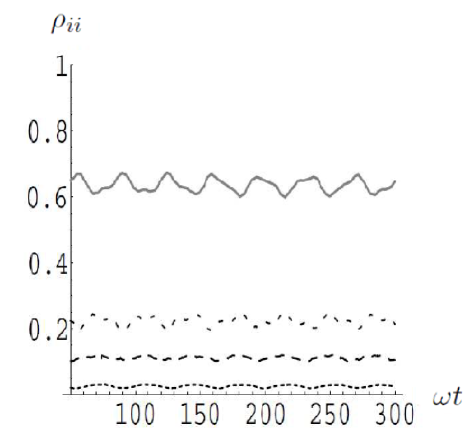
Figure 10: Time-asymptotic diagonal density matrix elements under moderate Spin-spin interaction ($\gamma^{\prime}=1$) in the Ising model coupling plotted against normalized time. Results similar to those in Figure 7, but with more ”noise”. However, there is an overall decoherence as a result of the coupling. The diagonal matrix elements are from top to bottom for $Uu,Lu,Ul,Ll$. For the parameter set:[$E=5,e=0.1,K=4,k=2.5,\omega=1,\gamma=0,\gamma^{\prime}=-0.5$]

3.3.1 Remarkable appearance of ”revivals”

”Revivals” or large amplitude - long period returns to the starting diagonal elements in the density of states have been shown in section 2.6 for a single qubit, Rabi model. Similar phenomena occur also in the two qubit case. While for most values of the parameters the diagonal density matrix elements exhibit only small oscillations over the time range in the asymptotic, long-time range, typically $\delta\rho\approx 1\%$, there are some singular values of the parameters where the oscillations are of the order of $100\%$ and persist over several periods.The periods are in the range of $50\cdot 2\pi/\omega$ or larger. An example of this behavior is shown in Figure 11 for the parameter set [$E=5,e=0.1,K=4,\omega=1,k=2.5$] at coupling strengths in the close vicinity of $\gamma^{\prime}=-0.5$, but not at more than about $0.02$ away from this value. Similar oscillations with comparable periods are observed for the parameter set [$E=5,e=0.1,K=2,k=1.25,\omega=1$], near the coupling strength value of $\gamma^{\prime}=.8$.

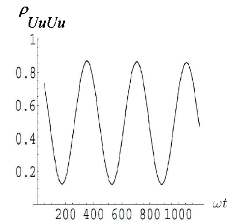
Figure 11: Large scale, large period ($>>2\pi/\omega$) oscillations in the diagonal Uu-component of the density matrix, superimposed on tiny $\approx 2\pi/\omega$ oscillations (not visible). Parameter values:[$E=5,e=0.1,K=4,k=2.5,\omega=1,\gamma=0,\gamma^{\prime}=-0.5$]

The oscillations are the more remarkable in that the time period of $300/\omega$, does not have any simple physical explanation in terms of the parameter set. (This is unlike the revival time expression in [12], holding for weak coupling and large $<N>$ case). Further investigation is needed to reveal the source of this result.

4 Discussion

In a two-qubit system whose energy-splittings are (respectively) much larger and much smaller than the frequencies in externally induced time-dependent perturbations, the low energy qubit decoheres, while the high energy qubit maintains its purity, being adiabatically protected. While this may be intuitively obvious, we have also examined less obvious cases when the two qubits are coupled and have found that for large coupling strength the adiabatic protection wears off.

The time averaging procedure used in the paper (introduced programatically in section 2.1) has been found to be in practice more time-economic for achieving the density matrix truncation than the mainstream formalism of environment tracing. A more basic advantage is that whereas in the latter method the truncation has to be enacted by some assumption of the nature and dynamics of the environment (e.g., the measuring apparatus, as in section 1.1.2 in [4]), which is outside and beyond the Hamiltonian of the system itself, in the present formalism the same effect is achieved by the relatively simple manipulation (time averaging) of the system’s Hamiltonians, as those in equation (1) and equation (9) -equation (12) , without speculating on the time development of the environment. In this sense, then, the system’s Hamiltonian is much more self-contained than that of the mainstream formalism. The choice of the time dependent terms in the above equations is apparently ad hoc and arbitrary; we have also tried in a preliminary way other forms (like a sum of oscillator terms, with random amplitudes and frequencies) and the results appear to be similar, except for the required time-width for averaging. To present these results in a systematic form represents an extension of the present (single frequency) model, which was indeed named ”A Minimal Model” in a recent presentation [38].

Another aspect for which the present formalism fills a gap is the distinction for the density matrix truncation, also discussed in section 1.1.2 of [4], between single run experiments (which are the ones frequently made in the laboratory and which are directly addressed by our formalism) and multiple run experiments (formalized by ensemble tracing). It is beyond the scope of the present work to investigate how time averaging in a single run is to be carried out in practice.

A further evident ramification of the time averaging formalism is in the direction of the second moments of the density matrix. (At present only the averages, or first moments, feature in our results.) This would be of importance, e.g., for expressing the ”basin of equilibration” (quantified in Eq. 8 of [39] through the ratio of the ”effective dimension explored” by the environment to the system’s environment), in terms of the parameters of our formalism.

References

- [1] 9
- [2] M. Schlosshauer, Rev. Mod. Phys. 76 1267 (2005)
- [3] R. Biele and R. D’Agosto, ”A Stochastic Approach to Open Quantum Systems” in Topical Reviews of the Journal of Physics: Condensed Matter 2̱4 273201 (2012); arXiv: 1112.2694 v3 [cond-mat.stat-mech] 1 Aug 2012
- [4] A.E. Allahverdyan, R. Balian and T.N. Niewenhuizen, ”Understanding quantum measurement from the solution of dynamical model” arXiv:11072.138v3 [quant-phys] 1Febr2013; Phys. Rep. 00(2013) 1-201
- [5] I. E. Farquhat, Ergodic Theory in Statistical Mechanics (Interscience, London, 1964) Chapter 2
- [6] R. Kubo, J. Math. Phys. 4174 (1963)
- [7] G. Gangopadhyay, M. S. Kumar and S. Dattagupta, J. Phys. A Math. Gen. 34 5485 (2001)
- [8] D. Lidar and J.B. Whaley, ”Decoherence-Free Subspaces and Subsystems” in Irreversible Quantum Dynamics, Springer Lecture Notes in Physics, No. 622 (Springer Verlag, Berlin, 2003) pp. 83-120, also arXiv.quant-ph /0301032
- [9] A. Aharony, O. Entin-Wohlman and S. Dattagupta, arXiv:0908.4385v1 [cond-mat.mes-hall] 30 Aug 2009
- [10] A. Aharony, S. Gurvitz, Y. Tokura, O. Entin-Wohlman and S. Dattagupta, arXiv:1205.5622v1 [cond-mat.mes-hall] 25 May 2012
- [11] I.I. Rabi, Phys. Rev. 49 324 (1936); ibid 51 652 (1937)
- [12] E.K. Irish, J. Gea-Banacloche, I. Martin and K.C. Schwab, Phys. Rev. B 72 195410 (2005)
- [13] S. Ashbab and F. Nori, Phys. Rev. A 81 042311 (2010)
- [14] D. Braak, Phys. Rev. Lett. 107 100401 (2011)
- [15] S. Agarwal, S.M. Hashemi Rafsanjani and J.H. Eberly, ArXiv:1201.2928v2[quant-ph] 9 Mar 2012
- [16] K. Ziegler, J. Phys. A. Math.THeor. 45 452001 (2012)
- [17] D. Leibfried, R. Blatt, C. Monroe and D. Wineland, Rev. Mod. Phys.75 281 (2003)
- [18] I. Thanopulos, E. Paspalakis and Z. Kis, Chem. Phys. Lett. 390 228 (2004)
- [19] A.T. Sornborger, A.N. Cleland and M.R. Geller, Phys. Rev. A 70 052315 (2004)
- [20] A. Wallraff et al, Nature 431 162 (2004); Phys. Rev. Lett. 95 060501 (2005)
- [21] P. Forn-Diaz et al, Phys. Rev. Lett. 105 237001 (2010)
- [22] M. Steffen et al, Science 313 1423 (2006)
- [23] P. Yang, P. Zou and Z.-M. Zhang, Phys. Lett. A 376 2977 (2012)
- [24] J. H. von Neumann, Mathematical Foundation of Quantum Mechanics (University Press,Princeton, 1955), Chapter III
- [25] W. Band, An Introduction to Quantum Statistics (Van Nostrand, Princeton,1955) Section 11.4
- [26] R. Englman and A. Yahalom, Phys. Rev. E 69 026120 (2004)
- [27] R. Gaspard and M. Nagaoka, J, Chem. Phys., 111 5668 (1999)
- [28] W.H. Zurek, S. Habib and J.P. Paz. Phys. Rev. Lett. 70 1187 (1993); W.H. Zurek, Progr. Theor. Phys. 89 281 (1993)
- [29] J.P. Paz and W.H. Zurek, Phys. Rev. Lett. 82 5181 (1999)
- [30] A. Leggett, S. Chakravarty, A. Dorsey, M. Fisher, A. Garg and W. Zwerger, Rev. Mod. Phys. 59 1 (1987)
- [31] R. Englman and A. Yahalom, Phys. Rev. B 69 224302 (2004)
- [32] R. Rechtman and O. Penrose, J. Stat. Phys. 19 359 (1978)
- [33] R. Englman, The Jahn-Teller Effect in Molecules and Crystals, (Wiley, London, 1972) Section 3
- [34] M.V. Feigel’man, L.R. Ioffe, V.E. Kravtsov and E. Cuevas, Ann. Phys. (N.Y.) 325 1390 (2010); M.V. Feigel’man, L.R. Ioffe and M. Mézard, Phys. Rev. B. 82 184534 (2010)
- [35] A. Daneri, A. Loinger and G.M. Prosperi, Nucl. Phys. 33 297 (1962)
- [36] A. Messiah, Quantum Mechanics (North Holland, Amsterdam, 1962), Vol.2, Chap. XVII, Sec. 11
- [37] R. Biele and R. D’Agosto, ”A Stochastic Approach to Open Quantum Systems” in Topical Reviews of the Journal of Physics: Condensed Matter 2̱4 273201 (2012); arXiv: 1112.2694 v3 [cond-mat.stat-mech] 1 Aug 2012
- [38] R. Englman and A. Yahalom, ”A Minimal Model for Decoherence and Thermalization by Ergodicity through Time Averaging” Israel Physical Society Annual Meeting, Jerusalem, Dec. 2012
- [39] N. Linden, S. Popescu, A.J. Short and A. Winter , Phys. Rev. E 79 061103 (2009)