Mechanical properties and microdomain separation of fluid membranes with anchored polymers

Abstract

The entropic effects of anchored polymers on biomembranes are studied using simulations of a meshless membrane model combined with anchored linear polymer chains. The bending rigidity and spontaneous curvature are investigated for anchored ideal and excluded-volume polymer chains. Our results agree with the previous theoretical predictions well. It is found that the polymer reduces the line tension of membrane edges, as well as the interfacial line tension between membrane domains, leading to microdomain formation. Instead of the mixing of two phases as seen in typical binary fluids, densely anchored polymers stabilize small domains. A mean field theory is proposed for the edge line tension reduced by anchored ideal chains, which well reproduces our simulation results.

I Introduction

Our knowledge of the heterogeneous structure of biomembranes has advanced from the primitive fluid mosaic model Singer72 to the modern raft model Simons97 ; Ikonen01 over the past decades. According to this modern model, membrane proteins are not randomly distributed in lipid membranes but concentrated in local microdomains, called lipid rafts, with a diameter of $10\sim 100$ nm Vereb03 ; Korade ; Pike . The raft contains high concentrations of glycosphingolipids and cholesterol, and plays important roles in many intra- and intercellular processes including signal transaction and membrane protein trafficking.

In the last decade, phase separation in multi-component lipid membranes has been intensively investigated in three-component systems of saturated and unsaturated phospholipids and cholesterol hone09 ; lipo03 ; baga09 ; Keller02 ; Tobias03 ; Hammond05 ; Kuzmin05 ; yana08 ; Schick09 . Lipid domains exhibit various interesting patterns on the micrometer scale, which can be reproduced by theoretical calculations and simulations. Various shapes of lipid domains can be also formed in the air–water interface mcco88 ; HaoWu09 ; iwam10 . However, the formation mechanism of microdomains on the $10\sim 100$ nm scale has not been understood so far. In lipid rafts, glycolipids contain glycan chains. Recently, network-shaped domains and small scattered domains have been observed in lipid membranes with PEG-conjugated cholesterol Miho12 . The effects of anchored polymers have been well investigated in the case of uniform anchoring on membranes, but the effects on the lipid domains and line tension have not been well investigated. In this paper, we focus on the effects of anchored polymers on the properties of biomembranes, in particular, on lipid domains.

It is well known that anchored polymers modify membrane properties. The polymer anchoring induces a positive spontaneous curvature $C_{0}$ of the membranes and increases the bending rigidity $\kappa$. These relations are analytically derived using the Green’s function method for mushroom region Lip95 ; Lip96 and confirmed by Monte Carlo simulations brei00 ; Auth03 ; Auth05 ; wern10 . The membrane properties in brush region are analyzed by scaling method Lip95 ; Lip96 ; Marsh03 . Experimentally, the $\kappa$ increase is measured by micropipette aspiration of liposomes Evans97 . Polymer decoration can enhance the stability of lipid membranes. PEG-conjugated lipids can reduce protein adsorption and adhesion on cellular surfaces, whereby PEG-coated liposomes can be used as a drug carrier in drug-delivery systems lasi94 ; hoff08 .

When vesicles are formed from the self-assembly of surfactant molecules via micelle growth, the vesicle size is determined kinetically by the competition between the bending energy and the line tension energy of the membrane edge helf74 ; from83 ; kale89 ; weis05 ; leng02 ; made11 ; brys05 ; nogu06a ; nogu13 . Recently, Bressel et al. reported that the addition of an amphiphilic copolymer induces the formation of larger vesicles bres12 . A polymer-anchoring-induced liposome-to-micelle transition is also observed Marsh03 ; scha02 ; john03 . The line tension of the membrane edge is considered to be reduced by polymer anchoring, but it has not been systematically investigated so far. In this study, we simulate the edge line tension for anchored ideal and excluded-volume chains and analytically investigate the polymer effects on the edge tension for ideal chains.

In order to simulate the polymer-anchoring effects on biomembranes, we employ one of the solvent-free meshless membrane models nog09 ; nog06 . Since we focus on the entropic effects of polymer chains, the detailed structures of the bilayer can be neglected, and thus the membranes can be treated as a curved surface. In the meshless model, a membrane particle represents a patch of bilayer membrane and membrane properties can be easily controlled.

In Sec. II, the membrane model and simulation method are described. In Sec. III, the bending rigidity and spontaneous curvature are estimated from the axial force measurement of cylindrical membranes and are also compared with the previous theoretical predictions. The reduction in the edge tension is discussed for both ideal chains and excluded-volume chains in Sec IV. In Sec V, we present our investigation how polymer anchoring modifies membrane phase separation. Finally, a summary and discussion are provided in Sec VI.

II Model and method

In this study, we employ a coarse-grained meshless membrane model nog06 with anchored linear polymer chains. One membrane particle possesses only translational degrees of freedom. The membrane particles form a quasi-two-dimensional (2D) membrane according to a curvature potential based on the moving least-squares (MLS) method nog06 . Polymer particles are linked by a harmonic potential, and freely move as a self-avoiding chain with a soft-core repulsion. One end of each polymer chain is anchored on a single membrane particle with a harmonic potential and a soft-core repulsion HaoWu13 . First, we simulate a single-phase membrane, where all membrane particles including polymer-anchored particles are the same type (A) of membrane particles. Then, we investigate membrane phase separation, where a membrane consists of two types (A and B) of membrane particles. The polymers are anchored to the type A particles.

We consider a single- or multi-component membrane composed of $N_{\rm{mb}}$ membrane particles. Among them, $N_{\rm{chain}}$ membrane particles are anchored by polymer chains. Each polymer chain consists of $N_{\rm{p}}$ polymer beads with an anchored membrane particle. The membrane and polymer particles interact with each other via a potential

$$U_{\rm{tot}}=U_{\rm{rep}}+U_{\rm{mb}}+U_{\rm{p}}+U_{\rm{AB}},$$ (1)

where $U_{\rm{rep}}$ is an excluded-volume potential, $U_{\rm{mb}}$ is a membrane potential, $U_{\rm{p}}$ is a polymer potential, and $U_{\rm{AB}}$ is a repulsive potential between different species of membrane particles.

All particles have a soft-core excluded-volume potential with a diameter of $\sigma$.

$$\frac{U_{\rm{rep}}}{k_{\rm B}T}=\varepsilon\sum_{i<j}\exp\left[-20(r_{ij}/\sigma-1)+B\right]f_{\rm{cut}}(r_{ij}/\sigma),$$ (2)

in which $k_{\rm B}T$ is the thermal energy and $r_{ij}$ is the distance between membrane (or polymer) particles $i$ and $j$. The diameter $\sigma$ is used as the length unit, $B=0.126$, and $f_{\rm{cut}}(s)$ is a $C^{\infty}$ cutoff function

$$f_{\rm{cut}}(s)=\left\{\begin{array}[]{ll}\exp\left\{A\left[1+\frac{1}{(|s|/s_{\rm{cut}})^{n}-1}\right]\right\}&(s<s_{\rm{cut}})\\ 0&(s\geqslant s_{\rm{cut}})\end{array}\right.$$ (3)

with $n=12$, $A=1$ and $s_{\rm{cut}}=1.2$.

For excluded-volume polymer chains, all pairs of particles including pairs of polymer beads have the repulsive interaction given in Eq. (2). In contrast, for ideal polymer chains, polymer beads have the excluded-volume interactions only with membrane particles to prevent polymer beads from passing through the membrane.

II.1 Meshless membrane model

The membrane potential $U_{\rm{mb}}$ consists of attractive and curvature potentials,

$$\frac{U_{\rm{mb}}}{k_{\rm B}T}=\sum_{i}^{N_{\rm{mb}}}\big{[}\varepsilon U_{\rm{att}}(\rho_{i})+k_{\alpha}\alpha_{\rm{pl}}({\mathbf{r}}_{i})\big{]},$$ (4)

where the summation is taken only over the membrane particles. The attractive multibody potential is employed to mimic the “hydrophobic” interaction.

$$U_{\rm{att}}(\rho_{i})=0.25\ln\left\{1+\exp\left[-4(\rho_{i}-\rho^{\ast})\right]\right\}-C,$$ (5)

which is a function of the local density of membrane particles $\rho_{i}=\sum_{j\neq i}^{N_{\rm{mb}}}f_{\rm{cut}}(r_{ij}/\sigma)$, with $s_{\rm{half}}=1.8$ and $s_{\rm{cut}}=s_{\rm{half}}+0.3$, where $f_{\rm{cut}}(s_{\rm{half}})=0.5$, which implies $A=\ln(2)\{(s_{\rm{cut}}/s_{\rm{half}})^{12}-1\}$. The constant $C$ is set for $U_{\rm{att}}(0)=0$. Here we use $\rho^{\ast}=6$ in order to simulate a 2D fluid membrane. For $\rho_{i}\lesssim\rho^{\ast}$, $U_{\rm{att}}$ acts as a pairwise potential with $U_{\rm{att}}=-2\sum_{j>i}f_{\rm{cut}}(r_{ij}/\sigma)$, and for $\rho_{i}\gtrsim\rho^{\ast}$, this potential saturates to the constant $-C$.

The curvature potential is expressed by the shape parameter called “aplanarity”, which is defined by

$$\alpha_{\rm{pl}}=\frac{9D_{\rm{w}}}{T_{\rm w}M_{\rm w}},$$ (6)

with the determinant $D_{\rm w}=\lambda_{1}\lambda_{2}\lambda_{3}$, the trace $T_{\rm w}=\lambda_{1}+\lambda_{2}+\lambda_{3}$, and the sum of the principal minors $M_{\rm w}=\lambda_{1}\lambda_{2}+\lambda_{2}\lambda_{3}+\lambda_{3}\lambda_{1}$. The aplanarity $\alpha_{\rm{pl}}$ scales the degree of deviation from the planar shape, and $\lambda_{1}$, $\lambda_{2}$, and $\lambda_{3}$ are three eigenvalues of the weighted gyration tensor

$$a_{\alpha\beta}({\mathbf{r}}_{i})=\sum_{j}^{N_{\rm{mb}}}(\alpha_{j}-\alpha_{G})(\beta_{j}-\beta_{G})w_{\rm{cv}}(r_{ij}),$$ (7)

where $\alpha,\beta\in\left\{x,y,z\right\}$, and the mass center of a local region of the membrane $\mathbf{r}_{G}=\sum_{j}\mathbf{r}_{j}w_{\rm{cv}}(r_{ij})/\sum_{j}w_{\rm{cv}}(r_{ij})$. A truncated Gaussian function is employed to calculate the weight of the gyration tensor

$$w_{\rm{cv}}(r_{ij})=\left\{\begin{array}[]{ll}\exp\left[\frac{(r_{ij}/r_{\rm{ga}})^{2}}{(r_{ij}/r_{\rm{cc}})^{12}-1}\right]&(r_{ij}<r_{cc})\\ 0&(r_{ij}\geqslant r_{\rm{cc}}),\end{array}\right.$$ (8)

which is smoothly cut off at $r_{ij}=r_{\rm{cc}}$. Here we use the parameters $r_{\rm{ga}}=0.5r_{\rm{cc}}$ and $r_{\rm{cc}}=3\sigma$. The bending rigidity and the edge tension are linearly dependent on $k_{\alpha}$ and $\varepsilon$, respectively, for $k_{\alpha}\gtrsim 10$, so that they can be independently varied by changing $k_{\alpha}$ and $\varepsilon$, respectively.

II.2 Anchored Polymer Chain

We consider flexible linear polymer chains anchored on the membrane. Polymer particles are connected by a harmonic spring potential,

$$\frac{U_{\rm{p}}}{k_{\rm B}T}=\frac{k_{\rm{bond}}}{2}\sum_{\rm chains}(r_{i,i+1}-b)^{2},$$ (9)

where $k_{\rm{bond}}$ is the spring constant for the harmonic potential and $b=1.2\sigma$ is the Kuhn length of the polymer chain. The summation is taken only between neighboring particles along polymer chains and between the end polymer particles and anchored membrane particles (a total of $N_{\rm p}$ springs in each chain).

II.3 Phase separation in membranes

Two types of membrane particles, A and B, are considered in Sec. V. The number of these particles are $N_{\rm A}$ and $N_{\rm B}$, respectively. To investigate phase separation, we apply a repulsive term $U_{\rm{AB}}$ in Eq. (1) to reduce the chemical affinity between different types of membrane particles. nog12 The potential $U_{\rm{AB}}$ is a monotonic decreasing function: $U_{\rm{AB}}/k_{\rm B}T=\varepsilon_{\rm{AB}}\sum_{i\in A,j\in B}A_{1}f_{\rm{cut}}(r_{i,j})$ with $n=1$, $A_{1}=1$ and $r_{\rm{cut}}=2.1\sigma$, and $A_{1}=\exp[\sigma/(r_{\rm{cut}}-\sigma)]$ to set $U_{\rm{AB}}(\sigma)=1$.

II.4 Simulation method

The $NVT$ ensemble (constant number of particles $N$, volume $V$, and temperature $T$) is used with periodic boundary conditions in a simulation box of dimensions $L_{x}\times L_{y}\times L_{z}$. For planar membranes, the projected area $L_{x}\times L_{y}$ is set for the tensionless state. The dynamics of both membrane and anchored flexible polymers are calculated by using underdamped Langevin dynamics. The motions of membrane and polymer particles are governed by

$$m\frac{d^{2}\mathbf{r}_{i}}{dt^{2}}=-\frac{\partial U_{\rm{tot}}}{\partial\mathbf{r}_{i}}-\zeta\frac{d\mathbf{r}_{i}}{dt}+\mathbf{g}_{i}(t),$$ (10)

where $m$ is the mass of a particle (membrane or polymer particle) and $\zeta$ is the friction constant. $\mathbf{g}_{i}(t)$ is a Gaussian white noise, which obeys the fluctuation-dissipation theorem. We employ the time unit $\tau=\zeta\sigma^{2}/k_{\rm B}T$ with $m=\zeta\tau$. The Langevin equations are integrated by the leapfrog algorithm alle87 with a time step of $\Delta t=0.005\tau$.

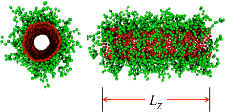
Figure 1: Front and side views of a snapshot of a cylindrical membrane with anchored excluded-volume polymer chains at the polymer density $\phi=0.167$ and cylinder axial length $L_{z}=45.3\sigma$. The red and green particles represent membrane and polymer particles, respectively.

We use $N_{\rm p}=10$, $\varepsilon=4$, $k_{\alpha}=10$, and $k_{\rm{bond}}=10$ throughout this study. In the absence of anchored polymer chains, the tensionless membranes have a bending rigidity of $\kappa/k_{\rm B}T=21\pm 0.5$, the edge tension $\Gamma_{\rm{ed}}\sigma/k_{\rm B}T=4.5$ and the area $a_{0}=1.44\sigma^{2}$ per membrane particle Hay11 . For the single-phase membranes, the number of membrane particles is fixed as $N_{\rm{mb}}=1200$ and the number fraction $\phi=N_{\rm{chain}}/N_{\rm{mb}}$ of polymer-anchored membrane particles is varied. To investigate phase separation, the number of the type A membrane particles is fixed as $N_{\rm{A}}=400$, and the number of the type B particles is chosen as $N_{\rm{B}}=400$ and $2100$ for a striped domain and a circular domain, respectively. The polymer chains are anchored to the type A particles and the polymer fraction $\phi=N_{\rm{chain}}/N_{\rm{A}}$ is varied. To confirm that the membranes are in thermal equilibrium, we compare the results between two initial states, stretching or shrinking, and check that no hysteresis has occurred. We slowly stretch and shrink cylindrical or striped membranes in the axial direction with a speed less than $dL_{z}/dt=10^{-6}\sigma/\tau$ and then equilibrate them for $t/\tau=6\times 10^{4}$ before the measurements. For the simulations of circular domains, the membranes were equilibriated for a duration of $6\times 10^{4}\tau$ after step-wise changes of $\varepsilon_{\rm{AB}}$. The error bars are calculated from six independent runs.

III Bending rigidity and spontaneous curvature of membranes

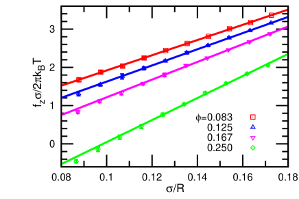
Figure 2: Force $f_{z}$ dependence on the radius $R$ of the cylindrical membranes with anchored excluded-volume chains at $\phi=0.083$, $0.125$, $0.167$, and $0.250$. The solid lines are obtained by linear least-squares fits.

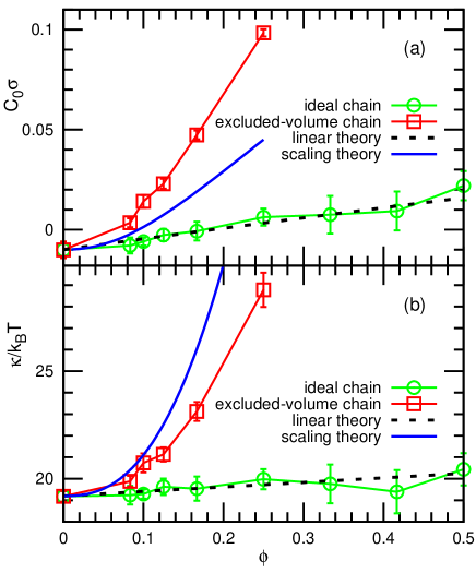
Figure 3: Polymer density $\phi$ dependence of (a) the spontaneous curvature $C_{0}$ and (b) bending rigidity $\kappa$ of the membranes with anchored ideal chains and excluded-volume chains. The dashed lines in (a) and (b) represent the prediction of the linear theory (Eqs. (14) and (15)) for the ideal chains. The solid lines in (a) and (b) represent the prediction of the scaling theory (Eqs. (16) and (17) ) in the brush region.

A cylindrical membrane with polymer chains anchored outside the membrane is used to estimate the polymer-induced spontaneous curvature and bending rigidity (see Fig. 1). For a cylindrical membrane with radius $R$ and length $L_{z}$, the Helfrich curvature elastic free energy is given by

$$F_{\rm{cv}} = \int\Big{[}\frac{\kappa}{2}(C_{1}+C_{2}-C_{0})^{2}+\bar{\kappa}C_{1}C_{2}\Big{]}dA$$ (11)

$$= 2\pi RL_{z}\left[\frac{\kappa}{2}\left(\frac{1}{R}-C_{0}\right)^{2}\right],$$

where $C_{1}$ and $C_{2}$ are the principal curvatures at each position on the membrane surface, and the membrane area $A=2\pi RL_{z}$. The coefficients $\kappa$ and $\bar{\kappa}$ are the bending rigidity and the saddle-splay modulus, respectively, and $C_{0}$ is the spontaneous curvature. In the absence of the anchored polymers (we call it a pure membrane hereinafter), the membrane has zero spontaneous curvature, $C_{0}=0$.

The membrane also has an area compression energy $F_{\rm{ar}}(A)$: $F_{\rm{ar}}(A)=K_{A}(A-A_{0})^{2}/2A_{0}$ for $A-A_{0}\ll A_{0}$, where $A_{0}$ is the area of the tensionless membrane. The radius $R$ is determined by free-energy minimization $\partial F/\partial R|_{L_{z}}=0$ for $F=F_{\rm{cv}}+F_{\rm{ar}}(A)$. Since the curvature energy increases with increasing $L_{z}$, a contractile force,

$$f_{z}=\frac{\partial F}{\partial L_{z}}\Big{|}_{R}=2\pi\kappa\Big{(}\frac{1}{R}-C_{0}\Big{)},$$ (12)

is generated along the cylindrical axis.

Figure 2 shows the axial force $f_{z}$ calculated from the pressure tensors,

$$P_{\alpha\alpha}=(Nk_{\rm B}T-\sum_{i}\alpha_{i}\frac{\partial U}{\partial{\alpha}_{i}})/V,$$ (13)

for $\alpha\in\{x,y,z\}$, where the summation is taken over all membrane and polymer particles. When the potential interaction crosses the periodic boundary, the periodic image $\alpha_{i}+nL_{\alpha}$ is employed for $P_{\alpha\alpha}$ calculation. The force $f_{z}$ increases linearly with $1/R$ HaoWu13 . Thus, $C_{0}$ and $\kappa$ of the anchored membranes can be estimated from a linear fitting method to Eq.  (12). For both anchored ideal chains and excluded-volume chains, the obtained values of $C_{0}$ and $\kappa$ are shown in Fig. 3. For the pure membranes, the value of $\kappa$ agrees very well with those estimated from the height fluctuations of planar membranes Hay11 and membrane buckling nogu11a . The estimated value of $C_{0}$ for the pure membrane deviates slightly from the exact value, zero. This small deviation would be caused by a higher-order term of the curvature energy harm06 or finite size effects as discussed in Ref. Hay11 .

The anchored polymer generates a positive spontaneous curvature, and enhances the bending rigidity $\kappa$. Both quantities increase with increasing polymer chain density, and for the excluded-volume chains, these increases are enhanced by the repulsive interactions between the neighboring chains.

In the mushroom region, the spontaneous curvature and bending rigidity are linearly dependent on the polymer density $\phi$. Analytically, the relations Lip95 ; Lip96

$$\kappa\Delta C_{0} = 2a_{\rm{sp}}k_{\rm B}TR_{\rm{end}}\phi/a_{0},$$ (14)

$$\Delta\kappa = a_{\kappa}k_{\rm B}TR_{\rm{end}}^{2}\phi/a_{0},$$ (15)

are predicted, where $\Delta C_{0}$ and $\Delta\kappa$ are the differences of the spontaneous curvatures and bending rigidities between the polymer-decorated membrane and the pure membrane, respectively, and $R_{\rm{end}}$ is the mean end-to-end distance of the polymer chain. The factor $2$ in Eq. (14) appears because in our definition the spontaneous curvature is twice as large as that in the previous works Lip95 ; Lip96 ; brei00 ; Auth03 . The coefficients are derived analytically using the Green’s function Lip95 ; Lip96 and also estimated by Monte Carlo simulations of single anchored polymer chains Auth03 : $a_{\kappa}=0.21$ and $0.2$; and $a_{\rm{sp}}=0.18$ and $0.17$ for ideal and excluded-volume chains, respectively. Our results for the ideal chains agree very well with these previous predictions (compare the dashed lines and symbols in Fig. 3). To draw the dashed line in Fig. 3(a), the end-to-end distance is estimated from the simulation; $R_{\rm{end}}=4.16\sigma$, which is slightly larger than a free polymer chain $R_{\rm{end}}=\sqrt{N_{\rm p}}b=3.79\sigma$. Note that anchored ideal polymer chains are in the mushroom region for any density $\phi$, since the polymer chains do not directly interact with each other.

For excluded-volume chains, our results deviate from the theoretical predictions (Eq. (14)) for the mushroom region at $\phi\gtrsim 0.1$. Thus, in the high density of anchored polymer chains, the interactions between polymer chains are not negligible. We compare our results with a scaling theory based on a blob picture for the brush region in Ref. Lip96 . For a cylindrical membrane, the spontaneous curvature is derived from the free-energy minimization with respect to the radius of the cylinder, Lip96

$$\frac{\partial f_{\rm c}(x)}{\partial x}+\frac{4\kappa_{0}}{k_{\rm B}T}N_{\rm p}^{-3}\bar{\Gamma}^{-3/2\nu}x=0,$$ (16)

where $f_{\rm c}(x)=[\{1+(1+\nu)x/\nu\}^{\nu/(1+\nu)}-1]/x-1$, the bending rigidity $\kappa_{0}$ of the pure membrane, and the reduced spontaneous curvature $x=h_{0}C_{0}/2$ for the height of a brush on a flat surface $h_{0}=N_{\rm p}\bar{\Gamma}^{(1-\nu)/2\nu}b$. The polymer coverage on the membrane is normalized by the maximum coverage as $\bar{\Gamma}=\Gamma/\Gamma_{\rm{max}}=b^{2}\phi/a_{0}$, and the exponent $\nu=0.6$ is used for excluded-volume chains. The bending rigidity is given by

$$\Delta\kappa=\frac{\nu+2}{12\nu^{2}}N_{\rm p}^{3}\bar{\Gamma}^{3/2\nu}k_{\rm B}T,$$ (17)

in the small curvature limit. Lip96 Our results qualitatively agree with these predictions from the scaling theory (see Fig. 3). The deviation is likely due to the polymer length ($N_{\rm p}=10$) in the simulation, which is too short to apply the blob picture in the scaling theory.

IV Edge line tension

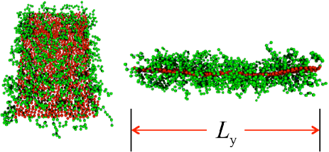
Figure 4: Top and side views of a snapshot of a membrane strip with anchored excluded-volume chains at $\phi=0.15$ and the length $L_{y}=57.6\sigma$ of each membrane edge.

IV.1 Simulation results

Next, we investigate the edge line tension with various anchored polymer densities for both ideal chains and excluded-volume chains. A strip of single-phase membrane with anchored polymers is used to estimate the edge tension $\Gamma_{\rm{ed}}$ (see Fig. 4). The edge tension $\Gamma_{\rm{ed}}$ can be calculated by Hay11 ; Briels04 ; Deserno08

$$\Gamma_{\rm{ed}}=\frac{\partial F}{2\partial L_{y}}=\Big{\langle}\frac{P_{xx}+P_{zz}}{2}-P_{yy}\Big{\rangle}\frac{L_{x}L_{z}}{2},$$ (18)

since the total edge length is $2L_{y}$. The pressure $P_{xx}=P_{zz}\approx 0$ for solvent-free simulation with a negligibly low critical micelle concentration. We checked that the edge tension is independent of the edge length for pure membranes as well as for polymer-decorated membranes (see Fig. 5).

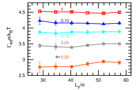
Figure 5: Edge line tension $\Gamma_{\rm{ed}}$ of a membrane strip with anchored excluded-volume chains estimated for different edge lengths $L_{y}$ at $\phi=0$, $0.1$, $0.15$, $0.2$, and $0.25$.

Figure 6 shows that the edge tension $\Gamma_{\rm{ed}}$ decreases with increasing polymer density $\phi$. The reduction for excluded-volume chains is much larger than that for ideal chains, similar to polymer effects on the bending rigidity. The polymer chains prefer staying on the edge, since there is more space to move so that they can gain entropy. Figure 7(a) shows that the polymer density distribution $\rho_{\rm{chain}}$ is nonuniform at the distance $d_{\rm w}$ from the strip’s central axis. High peaks of $\rho_{\rm{chain}}$ are found close to the edges for both ideal chains and excluded-volume chains, while the density $\rho_{\rm{mb}}$ of all membrane particles has only very small peak. The relative polymer density $\rho_{\rm{chain}}/\rho_{\rm{mb}}$ more rapidly increases at the edges for larger mean density $\phi$ [see Fig.  7(b)]. The mean polymer density $\phi_{1}$ at the edges is calculated as an average $\langle\sum_{d_{\rm w}\geq d_{\rm w}^{\rm{max}}}\rho_{\rm{chain}}/\sum_{d_{\rm w}\geq d_{\rm w}^{\rm{max}}}\rho_{\rm{mb}}\rangle$ for the right region of the peak ($d_{\rm w}^{\rm{max}}$) of $\rho_{\rm{mb}}$ in Fig. 7(a). The density difference from the mean value $\Delta\phi=\phi_{1}-\phi$ increases with increasing $\phi$ as shown in Fig. 8. The excluded volume chains induce higher polymer concentration at the edges than the ideal chains.

IV.2 Theoretical analysis

Here we propose a mean field theory for the edge line tension induced by the anchored polymers in the mushroom region. According to the nonuniform polymer distribution on the membrane strip, we divide the membrane into two regions, an edge (region 1) and middle region (region 2). The polymer density is assumed to be uniform in each region. The area fractions of the two regions are $n_{1}$ and $n_{2}$ with $n_{1}+n_{2}=1$, and the polymer densities are $\phi_{1}$ and $\phi_{2}$ with $\phi=n_{1}\phi_{1}+n_{2}\phi_{2}$. The width of region 1 is considered the radius of gyration of polymer $R_{\rm g}$, so that the area fraction is given by

$$n_{1}=\frac{2L_{y}R_{\rm g}}{N_{\rm{mb}}a_{0}}.$$ (19)

The free energy of the membrane strip is written as

$$\frac{F_{\rm{ed}}}{N_{\rm{mb}}k_{\rm B}T} = n_{1}\phi_{1}\ln\phi_{1}+n_{1}\left(1-\phi_{1}\right)\ln\left(1-\phi_{1}\right)$$ (20)

$$+n_{2}\phi_{2}\ln\phi_{2}+n_{2}\left(1-\phi_{2}\right)\ln\left(1-\phi_{2}\right)$$

$$-n_{1}\phi_{1}\Delta S+f_{0},$$

where $f_{0}$ is the free energy contribution of the membrane without polymer anchoring. The first four terms are the mixing entropy for regions 1 and 2. When a polymer chain moves from the middle region to the open edges, it gains the conformational entropy $\Delta S$.

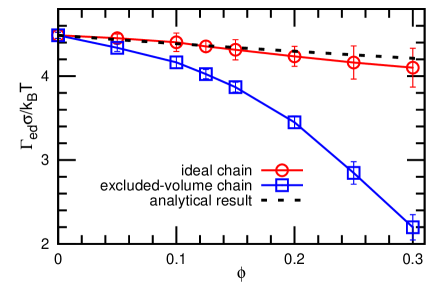
Figure 6: Polymer density dependence $\phi$ of the edge line tension for ideal and excluded-volume chains. The dashed line represents our theoretical prediction by Eq. (23).

The partition function of a single anchored polymer chain is expressed as $Z_{\rm p}=q^{N_{\rm p}}W$, where $q$ is the number of the nearest neighbors in the lattice model ($q=6$ in a cubic lattice). The restricted weight of a polymer anchored on the flat membrane is $W_{\rm{hs}}={\rm{erf}}\left[\frac{\sqrt{q}l_{\rm{an}}}{2R_{\rm{end}}}\right]$, where erf$(x)$ is the error function and $l_{\rm{an}}$ is the anchor length Lip95 ; Lip96 . On the other hand, the free end of a polymer anchored on the edge can also move in the other half space, and has a larger value of weight $W_{\rm{ed}}$. We numerically counted the weights $W_{\rm{ed}}$ and $W_{\rm{hs}}$ in a cubic lattice. The ratio $W_{\rm{ed}}/W_{\rm{hs}}$ increases with increasing $N_{\rm p}$, and $W_{\rm{ed}}/W_{\rm{hs}}\simeq 2$ for $N_{\rm p}=10$. Thus, the excess entropy is estimated as $\Delta S=\ln\left(W_{\rm{ed}}/W_{\rm{hs}}\right)\simeq\ln 2$ for our simulation condition.

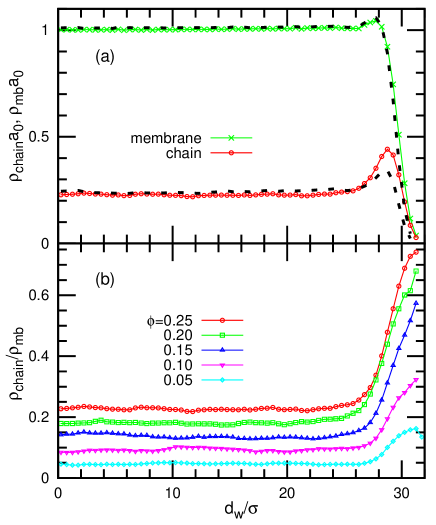
Figure 7: Density distribution in the membrane strip. (a) Density of polymer-anchored membrane particles $\rho_{\rm{chain}}$, and total density $\rho_{\rm{mb}}$ at $\phi=0.25$. The solid lines with symbols and dashed lines represent the data for the excluded-volume chains, and ideal chains, respectively. (b) Density ratio $\rho_{\rm{chain}}/\rho_{\rm{mb}}$ for the excluded-volume chains. The distance $d_{\rm w}$ from the center of the strip is taken in the direction perpendicular to the edge. The membrane lengths are $L_{\rm{st}}=60\sigma$ perpendicular to the edge and $L_{y}=28.8\sigma$ along the edge.

Figure 8: Excess polymer density $\Delta\phi\equiv\phi_{1}-\phi$ at the membrane edge as a function of the mean polymer density $\phi$. The solid lines with circles and squares represent our simulation results for the ideal chains and excluded volume chains, respectively. The dashed line represents our theoretical prediction for the ideal chains by Eq. (IV.2).

Using minimization of $F_{\rm{ed}}$, the polymer density $\phi_{1}$ in the edge region is analytically derived as

$$\phi_{1} = \frac{2Q\phi}{s+\sqrt{s^{2}-4Q(Q-1)\phi n_{1}}}$$

$$= \frac{Q\phi}{1+(Q-1)\phi}\Bigg{(}1-\frac{(Q-1)(1-\phi)}{\{1+(Q-1)\phi\}^{2}}n_{1}\Bigg{)}+O(n_{1}^{2}),$$

where $Q=\exp(\Delta S)$ and $s=1+(Q-1)(\phi+n_{1})$. At $Q=2$ and $n_{1}\ll 1$, the density difference is simply $\Delta\phi\equiv\phi_{1}-\phi=\phi(1-\phi)/(1+\phi)$, which agrees well with the simulation results (see Fig. 8).

The edge tension is derived as $\Gamma_{\rm{ed}}=\partial F_{\rm{ed}}/\partial L_{\rm{ed}}$, where $L_{\rm{ed}}$ is the total edge length $L_{\rm{ed}}=2L_{y}$. Thus, the polymer-induced edge tension $\Delta\Gamma_{\rm{ed}}$ is given by

$$\frac{\Delta\Gamma_{\rm{ed}}a_{0}}{R_{\rm g}k_{\rm B}T} = \ln(1-n_{1})+\phi_{1}\ln\frac{\phi_{1}}{Q(\phi-\phi_{1}n_{1})}$$

$$+(1-\phi_{1})\ln\frac{1-\phi_{1}}{1-\phi-(1-\phi_{1})n_{1}}.$$

At $Q=2$, the Taylor expansion gives

$$\frac{\Delta\Gamma_{\rm{ed}}a_{0}}{R_{\rm g}k_{\rm B}T}=-\ln(1+\phi)+\frac{\phi(1-\phi)}{(1+\phi)^{2}}n_{1}+O(n_{1}^{2}).$$ (23)

Thus, the edge tension $\Gamma_{\rm{ed}}$ decreases with increasing $\phi$ and is independent of the edge length $L_{y}$ for $n_{1}\ll 1$. Figure 6 shows the comparison of edge tensions between our simulation and the theoretical results for ideal chains; The agreement is excellent. As the membrane strip becomes narrower ($n_{1}$ increases), the polymer effect on the edge tension $\Gamma_{\rm{ed}}$ is reduced by the loss of mixing entropy in region 2, and $\Gamma_{\rm{ed}}$ increases with increasing edge length $L_{y}$.

For the excluded-volume polymer chains, the membrane cannot be simply divided into two regions because of the repulsive interaction between polymer chains. The effects of the membrane edges may be considered as an increase in the average volume for each chain. For a flat membrane without edges, the volume per chain is given by $V_{\rm{pf}}=2R_{\rm{end}}L_{x}L_{y}/N_{\rm{chain}}$. The membrane strip has an additional space $\pi R_{\rm{end}}^{2}L_{y}$ around the edges so that the polymer volume becomes $V_{\rm{pe}}=V_{\rm{pf}}+\pi R_{\rm{end}}^{2}L_{y}/N_{\rm{chain}}$. Thus, the polymer chains gain additional conformational entropy not only at the edges but in the middle of the strip.

V Membrane domains with anchored polymers

In this section, we focus on the effects of anchored polymers on membrane phase separation. First, in Sec. V.1 we estimate the line tension of polymer-anchored membrane domains, and then in Sec. V.2 we investigate the polymer effects on domain separation and domain shape transformation. Here, we investigate only the membranes with excluded-volume chains, since the effects of the ideal chains are considered to be very small. As described in Sec. III, polymers can induce an effective spontaneous curvature in the membrane. In order to diminish the influence of the induced spontaneous curvature, we symmetrically anchor polymer chains on both sides of the membrane as shown in Fig. 9. Half of the chains ($N_{\rm{chain}}/2$) are anchored on the upper (lower) side of the membrane, and each chain is anchored on one membrane particle. Then, the net curvature effects induced on both sides of the membrane cancel each other out.

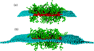
Figure 9: Snapshots of (a) striped and (b) circular domains with anchored excluded-volume chains in planar membranes at $N_{\rm A}=400$ and $\phi=0.3$. Type A and B membrane particles are displayed in red and blue, respectively.

V.1 Interfacial line tension between two membrane domains

The line tension $\Gamma_{\rm{AB}}$ between the type A and B domains is estimated by two methods using a striped domain and a circular domain. For the striped domain shown in Fig. 9$(a)$, the line tension is calculated by

$$\Gamma_{\rm{AB}}=\langle P_{xx}-P_{yy}\rangle L_{x}L_{z}/2.$$ (24)

The obtained line tension for tensionless membranes is shown by solid lines in Fig. 10. We ensured that $\Gamma_{\rm{AB}}$ is independent of the boundary length $L_{y}$ for $24<L_{y}/\sigma<48$ (data not shown). The line tension $\Gamma_{\rm{AB}}$ decreases with increasing $\phi$, while $\Gamma_{\rm{AB}}$ increases with increasing $\varepsilon_{\rm{AB}}$. Thus, the same value of $\Gamma_{\rm{AB}}$ can be obtained for different polymer densities $\phi$ by adjusting $\varepsilon_{\rm{AB}}$.

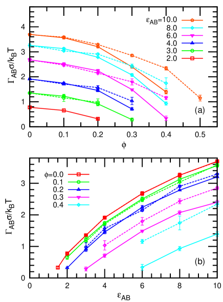
Figure 10: Interfacial line tension $\Gamma_{\rm{AB}}$ between membrane domains as a function of (a) $\phi$ and (b) $\varepsilon_{\rm{AB}}$. The solid and dashed lines represent $\Gamma_{\rm{AB}}$ estimated from the striped domain and the circular domain, respectively.

Before investigating polymer effects on the domain shapes in the next subsection, we also estimate $\Gamma_{\rm{AB}}$ from the circular domain shown in Fig. 9$(b)$. The line tension $\Gamma_{\rm{AB}}$ is calculated by the 2D Laplace pressure, Briels04 ; nog12

$$\Gamma_{\rm{AB}}=\bar{R}\Delta\gamma,$$ (25)

where $\bar{R}$ is the average radius of the domain, and $\Delta\gamma$ is the difference of surface tension between the type A and B domains: $\Delta\gamma=\gamma^{\rm{in}}-\gamma^{\rm{out}}$, where $\gamma^{\rm{in}}$ is the surface tension of the inner (type A) domain and $\gamma^{\rm{out}}$ is that of the outer (type B) domain. Both of them can be estimated by the pressure tensors of the local regions

$$\gamma^{\rm{\alpha}}=\langle P^{\rm{\alpha}}_{zz}-(P^{\rm{\alpha}}_{xx}+P^{\rm{\alpha}}_{yy})/2\rangle L_{z},$$ (26)

where $\alpha$ represents “in” or “out”; $P^{\rm{\alpha}}_{xx}$, $P^{\rm{\alpha}}_{yy}$, and $P^{\rm{\alpha}}_{zz}$ are the diagonal components of the pressure tensors calculated in the local membrane regions. The outer surface tension $\gamma^{\rm{out}}$ can also be calculated from the pressure tensors for the whole area.

To estimate $\gamma^{\rm{in}}$ and $\gamma^{\rm{out}}$, we extract the inner and outer regions as follows. First, domains of type A particles are calculated. The particles are considered to belong to the same cluster (domain) when their distance is less than $r_{\rm{cut}}=2.1\sigma$. Then the radius $\bar{R}$ of the largest domain is calculated. Type A particles contacting type B particles (closer than $r_{\rm{cut}}$) are considered domain boundary particles. The number of boundary particles is $N_{\rm{bd}}$. In the largest domain, the distance of the domain particles from the center ${\bf r}_{\rm G}$ of the domain is averaged by $R_{\rm A}=(1/N_{\rm{bd}})\sum|{\bf r}-{\bf r}_{\rm G}|$. For the mean radius of the domain boundary, the half boundary width $\sqrt{a_{0}}/2=0.6\sigma$ is added so that $\bar{R}=R_{\rm A}+0.6\sigma$. Then, the maximum fluctuation amplitude $\Delta R$ around $\bar{R}$ is calculated. The surface tension $\gamma^{\rm{in}}$ is estimated within the area inside the circular region with radius $\bar{R}-\Delta R-0.5\sigma$, while $\gamma^{\rm{out}}$ is estimated within the area outside the circular region with radius $\bar{R}+\Delta R+0.5\sigma$. Note that a few type B particles can enter the type A domain at small $\Gamma_{AB}\sigma/k_{\rm B}T\sim 1$ so the type A particles neighboring these isolated particles are not taken into account for estimation of $\bar{R}$ and $\Delta R$.

The line tension estimated from the 2D Laplace pressure is shown by dashed lines in Fig. 10. For the pure membrane, the obtained values agree with those from the membrane strip very well. However, they are slightly larger for the polymer-anchored membranes. This deviation is likely caused by the relative larger boundary region of the circular domain than the striped domain. It is a similar dependence obtained for the membrane edges (see Eq. (23)).

The phase behavior of the pure membranes ($\varepsilon_{\rm{AB}}=0$) belongs to the universality class of the 2D Ising model lipo92 . For the polymer-anchored membranes, however, the line tension dependence on the boundary curvature is not explained by the universality class. Thus, the polymer effects cannot be treated as an effective potential between neighboring membrane particles.

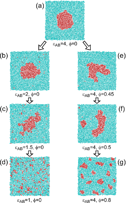
Figure 11: Sequential snapshots of domain separations as (left from (a) to (d)) $\varepsilon_{\rm{AB}}$ decreases at $\phi=0$ or (right from (a) to (g)) as the polymer density $\phi$ increases at $\varepsilon_{\rm{AB}}=4$. Red and blue particles represent the A and B type membrane particles, respectively. To show microdomain separation and shape transformation clearly, polymer particles are not displayed.

V.2 Domain separation and microdomain formation

Figure 12: Domain shape changes and domain separation as (a,b) $\varepsilon_{\rm{AB}}$ decreases at $\phi=0$ and (c,d) $\phi$ increases at $\varepsilon_{\rm{AB}}=4$. (a,c) The average cluster size $\bar{N}_{\rm{dm}}$ of the mother (largest) domains and (b,d) the reduced excess domain length $\Delta L_{\rm{bd}}$ of the mother domains. The mean number $N_{\rm{mth}}$ of the membrane particles in the mother domains at each stage is shown in light red color.

To clarify the anchored polymer effects, we compare the shape changes of the type A membrane domains with increasing $\phi$ and with decreasing $\varepsilon_{\rm{AB}}$. In both cases, the interfacial line tension $\Gamma_{\rm{AB}}$ decreases and the low line tension leads to the breakup of domains. However, the resultant states are quite different as shown in Fig. 11. As the repulsive interaction between the type A and B particles is reduced with decreasing $\varepsilon_{\rm{AB}}$, the obtained phase behavior is similar to that of typical binary fluids. At $\Gamma_{\rm{AB}}\sigma\simeq k_{\rm B}T$ ($\varepsilon_{\rm{AB}}=2$), the domain boundary undergoes large fluctuation and a few (type A or B) particles leave their domain to dissolve in the other domain. As $\varepsilon_{\rm{AB}}$ decreases further, the domain breaks up into small domains, and finally the two types of particles are completely mixed.

On the other hand, the anchored polymers induce formation of small stable domains (called microdomains) instead of a mixing state, although it can reduce the line tension to $\Gamma_{\rm{AB}}\sigma\lesssim k_{\rm B}T$ (see Fig. 11(g)). At $\phi\leq 0.45$, the type A domain remains as one domain but exhibits an elongated shape at $\phi=0.45$. At $\phi\geq 0.5$, it starts separating into microdomains. Note that the membrane is considered in a mixed state even at $\phi=0.45$, if $\Gamma_{\rm{AB}}$ for the straight boundary is extrapolated (see Fig. 10).

In contrast to the reduction in $\varepsilon_{\rm{AB}}$, the boundary of the elongated domain is rather smooth (compare snapshots in Figs. 11(c) and (f)). We confirmed that these small domains are also formed from random distribution of initial states. Thus, it is a thermodynamically stable state.

Let us discuss the effects of the polymer anchoring on the domain formation. First, we remind that the polymer beads have only repulsive interactions with the other beads and membrane particles except for the membrane-anchored head particles.

The polymer effects seem suppressed for shorter lengths than the polymer size $\sim R_{\rm{end}}=4\sigma$. A smaller boundary undulation than the polymer size does not yield additional space for the polymer brush. A similar suppression in the short length scale was reported on the bending rigidity induced by the polymer anchoring Auth05 . When the domain size is comparable to the polymer length, most of the particles already stay at the domain boundary, so that an additional increase in the boundary length likely yields much less gain in the average volume per polymer and the polymer conformational entropy. As explained in Sec. V.1, the line tension of the circular domain is larger than the straight boundary. For the smaller domains, this difference would be enhanced, although the domains are too small for direct estimation of $\Gamma_{\rm{AB}}$ by Laplace’s law.

To investigate the changes of domains in greater detail, we calculate the mean cluster size $\bar{N}_{\rm{dm}}$ and a reduced excess domain length $\Delta L_{\rm{bd}}$. The cluster size $\bar{N}_{\rm{dm}}$ is defined as

$$\bar{N}_{\rm{dm}}=\frac{\sum^{N_{\rm A}}_{i_{\rm c}=1}n_{i}i_{\rm c}^{2}}{\sum^{N_{\rm A}}_{i_{\rm c}=1}n_{i}i_{\rm c}},$$ (27)

where $n_{i}$ is the number of clusters with size $i_{\rm c}$. The reduced excess domain length for the mother (largest) domains $\Delta L_{\rm{bd}}$ is defined as

$$\Delta L_{\rm{bd}}=\frac{L_{\rm{bd}}}{2\sqrt{\pi A_{\rm{dm}}}}-1,$$ (28)

where $L_{\rm{bd}}=N_{\rm{bd}}\sqrt{a_{0}}$ is the boundary length of the mother domains and $A_{\rm{dm}}=N_{\rm A}a_{0}$ is the domain area. The length $L_{\rm{bd}}$ is normalized by the length of a circular domain $2\sqrt{\pi A_{\rm{dm}}}$ so that $\Delta L_{\rm{bd}}=0$ for the circular domain.

Figure 12 shows the development of $\bar{N}_{\rm{dm}}$ and $\Delta L_{\rm{bd}}$. In the $\varepsilon_{\rm{AB}}$ reduction, the transition to the mixing state occurs sharply between $\varepsilon_{\rm{AB}}=1.5$ and $1$. However, for polymer anchoring, a gradual decrease in $\bar{N}_{\rm{dm}}$ represents the formation of microdomains (see Fig. 12(c)). Around the transition points, $\Delta L_{\rm{bd}}$ is increased less by polymer anchoring than by lowering $\varepsilon_{\rm{AB}}$, while both domains are similarly elongated (see Fig. 11). This difference is caused by the weaker undulation of polymer-decorated domain boundaries.

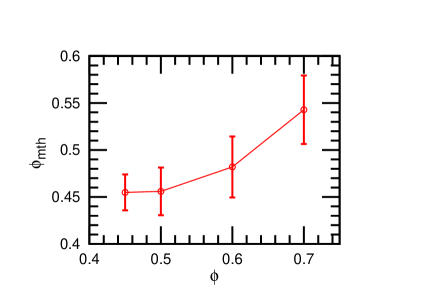
Figure 13: Mean polymer density $\phi$ dependence of the number fraction $\phi_{\rm{mth}}$ of polymer chain anchors on the mother (largest) domain.

We calculated the fraction of polymer chain anchors on the mother domain $\phi_{\rm{mth}}$ after the microdomain separation (see Fig. 13). Interestingly, it is lower than the initial density $\phi$. Thus, detached small domains have higher polymer densities than their mother domain. This is caused thermodynamically by the entropy gain of polymers anchored on small domains and also kinetically by a higher density at the domain boundary.

VI Summary and discussion

We have systematically studied the entropic effects of anchored polymers on various types of mechanical and interfacial properties of biomembranes using particle-based membrane simulations. First, we reconfirm the previous theoretical predictions for spontaneous curvature and bending rigidity by simulating cylindrical membranes. They increase with the anchored polymer density $\phi$ linearly in the mushroom region, but sharply increase in the brush region.

Second, we investigated the polymer anchoring effects on the edge line tension for ideal and excluded-volume chains. It is revealed that polymer anchoring significantly reduces the edge tension. For ideal polymer chains, it is also investigated by a mean field theory. It is clarified that the entropy gain of polymer conformation at the membrane edge reduces the edge tension. Experimentally, it is known that polymer anchoring induces the formation of large vesicles bres12 and spherical or discoidal micelles john03 . Since the ratio between the edge tension and the bending rigidity determines the vesicle radius $R_{\rm{ves}}$ formed by the membrane disks as $R_{\rm{ves}}\sim(2\kappa+\bar{\kappa})/\Gamma_{\rm{ed}}$, the reduction in the edge tension increases the vesicle radius. Our results are consistent with these experimental observations.

Finally, we investigated the polymer anchoring effects on phase separation in membranes for excluded-volume chains. The line tension of the domain boundary is reduced by anchoring polymers. It is found that densely anchored polymers can stabilize microdomains, whereas large domains are unstable. Although we did not investigate polymer length dependence here, it is expected that the domain size can be controlled by the polymer length. In living cells, lipid rafts contain a large amount of glycosphingolipids Vereb03 ; Korade ; Pike . Our simulation results suggest that the entropic effects of glycosphingolipids may play a significant role in stabilizing microdomains $\lesssim 100$ nm. At a moderate polymer density, elongated shapes of membrane domains are obtained. In lipid membranes with PEG-conjugated cholesterol, the domain shapes depend on the anchored polymer density $\phi_{\rm{PEG}}$: at a high $\phi_{\rm{PEG}}$, small domains are scattered, while at a slightly lower $\phi_{\rm{PEG}}$, small elongated domains are connected with each other to form a network Miho12 . The elongated domains in our simulations may form a network, if much larger domains are simulated. Further study is needed to clarify the polymer-anchoring effects on large-scale domain patterns.

Our present study highlights entropic effects of anchored polymers on the microdomain formation via the reduction in domain boundary tension on quasi-2D biomembranes. It is well known that high line tension can induce budding of membranes lipo03 ; baga09 ; lipo92 . Nonzero spontaneous curvature induced by proteins and anchored polymers can lead to various liposome shapes, such as tube formation and pearling baum11 ; phil09 ; shny09 ; tsaf01 ; akiy03 ; guo09 . Shape transformation of vesicles induced by polymer-decorated domains is an interesting topic for further studies.

VII Acknowledgments

We would like to thank G. Gompper, P. A. Pincus, T. Auth, T. Taniguchi, V. N. Manoharan, and S. Komura for informative discussions. This study is partially supported by KAKENHI (25400425) from the Ministry of Education, Culture, Sports, Science, and Technology (MEXT) of Japan. HW is supported by a MEXT scholarship.

References

- (1) S. J. Singer and G. L. Nicolson, Science, 175, 720 (1972).
- (2) K. Simons and E. Ikonen, Nature, 387, 569 (1997).
- (3) E. Ikonen, Curr. Opin. Cell Biol., 13, 470 (2001).
- (4) G. Vereb, J. Szöllősi, J. Matko, P. Nagy, T. Farkas, L. Vigh, L. Matyus, T. A. Waldmann and S. Damjanovich, Proc. Natl. Acad. Sci. USA, 100, 8053 (2003).
- (5) Z. Korade and A. K. Kenworthy, Neuropharmacology, 55, 1265 (2008).
- (6) L. J. Pike, J. Lipid Res., 50, S323 (2009).
- (7) A. R. Honerkamp-Smith, S. L. Veatch and S. L. Keller, Biochim. Biophys. Acta, 1788, 53 (2009).
- (8) R. Lipowsky and R. Dimova, J. Phys.: Condens. Matter, 15, S31 (2003).
- (9) L. Bagatolli and P. B. S. Kumar, Soft Matter, 5, 3234 (2009).
- (10) S. L. Veatch and S. L. Keller, Phys. Rev. Lett., 89, 268101 (2002).
- (11) T. Baumgart, S. T. Hess and W. W. Webb, Nature, 425, 821 (2003).
- (12) A. T. Hammond, F. A. Heberle, T. Baumgart, D. Holowka, B. Baird and G. W. Feigenson, Proc. Natl. Acad. Sci. USA, 102, 6320 (2005).
- (13) P. I. Kuzmin, S. A. Akimov, Y. A. Chizmadzhev, J. Zimmerberg and F. S. Cohen, Biophys. J., 88, 1120 (2005).
- (14) M. Yanagisawa, M. Imai and T. Taniguchi, Phys. Rev. Lett., 100, 148102 (2008).
- (15) G. G. Putzel and M. Schick, Biophys. J., 96, 4935 (2009).
- (16) H. M. McConnell and V. T. Moy, J. Phys. Chem., 92, 4520 (1988).
- (17) H. Wu and Z. C. Tu, J. Chem. Phys., 130, (2009).
- (18) M. Iwamoto, F. Liu and Z.-c. Ou-Yang, EPL, 91, 16004 (2010).
- (19) M. Yanagisawa, N. Shimokawa, M. Ichikawa and K. Yoshikawa, Soft Matter, 8, 488 (2012).
- (20) R. Lipowsky, Europhys. Lett., 30, 197 (1995).
- (21) C. Hiergeist and R. Lipowsky, J. Phys. II France, 6, 1465 (1996).
- (22) M. Breidenich, P. R. Netz, and R. Lipowsky, Europhys. Lett., 49, 431 (2000).
- (23) T. Auth and G. Gompper, Phys. Rev. E, 68, 051801 (2003).
- (24) T. Auth and G. Gompper, Phys. Rev. E, 72, 031904 (2005).
- (25) M. Werner and J.-U. Sommer, Eur. Phys. J. E, 31, 383 (2010).
- (26) D. Marsh, R. Bartucci, and L. Sportelli, Biochim. Biophys. Acta, 1615, 33 (2003).
- (27) E. Evans and W. Rawicz, Phys. Rev. Lett., 79, 2379 (1997).
- (28) D. D. Lasic, Angew. Chem. Int. Ed. Engl., 33, 1685 (1994).
- (29) A. S. Hoffman, J. Control. Release, 132, 153 (2008).
- (30) W. Helfrich, Phys. Lett. A, 50, 115 (1974).
- (31) P. Fromherz, Chem. Phys. Lett., 94, 259 (1983).
- (32) E. W. Kaler, A. K. Murthy, B. E. Rodriguez, and J. A. N. Zasadzinski,Science, 245, 1371 (1989).
- (33) T. M. Weiss, T. Narayanan, C. Wolf, M. Gradzielski, P. Panine, S. Finet, and W. I. Helsby, Phys. Rev. Lett., 94, 038303 (2005).
- (34) J. Leng, S. U. Egelhaaf, and M. E. Cates, Europhys. Lett., 59, 311 (2002).
- (35) D. Madenci, A. Salonen, P. Schurtenberger, J. S. Pedersen, and S. U. Egelhaaf, Phys. Chem. Chem. Phys., 13, 3171 (2011).
- (36) K. Bryskhe, S. Bulut, and U. Olsson, J. Phys. Chem. B, 109, 9265 (2005).
- (37) H. Noguchi and G. Gompper, J. Chem. Phys., 125, 164908 (2006).
- (38) H. Noguchi, J. Chem. Phys., 138, 024907 (2013).
- (39) K. Bressel, M. Muthig, S. Prevost, J. Gummel, T. Narayanan, and M. Gradzielski, ACS Nano, 6, 5858 (2012).
- (40) A. Schalchli-Plaszczynski and L. Auvray, Eur. Phys. J. E, 7, 339 (2002).
- (41) M. Johnsson and K. Edwards, Biophys. J., 85, 3839 (2003).
- (42) H. Noguchi, J. Phys. Soc. Jpn., 78, 041007 (2009).
- (43) H. Noguchi and G. Gompper, Phys. Rev. E, 73, 021903 (2006).
- (44) H. Wu and H. Noguchi, AIP Conf. Proc., 1518, 649 (2013).
- (45) H. Noguchi, Soft Matter, 8, 8926 (2012).
- (46) M. P. Allen and D. J. Tildesley, Computer Simulation of Liquids, Clarendon Press, Oxford (1987).
- (47) H. Shiba and H. Noguchi, Phys. Rev. E, 84, 031926 (2011).
- (48) H. Noguchi, Phys. Rev. E, 83, 061919 (2011).
- (49) V. A. Harmandaris and M. Deserno, J. Chem. Phys., 125, 204905 (2006).
- (50) T. V. Tolpekina, W. K. den Otter, and W. J. Briels, J. Chem. Phys., 121, 8014 (2004).
- (51) B. J. Reynwar and M. Deserno, Biointerphases, 3, FA117 (2008).
- (52) R. Lipowsky, J. Phys. II France, 2, 1825 (1992).
- (53) R. Phillips, T. Ursell, P. Wiggins, and P. Sens, Nature, 459, 379 (2009).
- (54) A. V. Shnyrova, V. A. Frolov, and J. Zimmerberg, Curr. Biology, 19, R772 (2009).
- (55) I. Tsafrir, D. Sagi, T. Arzi, M.-A. Guedeau-Boudeville, V. Frette, D. Kandel, and J. Stavans, Phys. Rev. Lett., 86, 1138 (2001).
- (56) K. Akiyoshi, A. Itaya, S. M. Nomura, N. Ono, and K. Yoshikawa, FEBS Lett., 534, 33 (2003).
- (57) K. Guo, J. Wang, F. Qiu, H. Zhang, and Y. Yang, Soft Matter, 5, 1646 (2009).
- (58) T. Baumgart, B. R. Capraro, C. Zhu, and S. L. Das, Annu. Rev. Phys. Chem., 62, 483 (2011).