Asymmetric Ferromagnetic Resonance, Universal Walker Breakdown, and Counterflow Domain Wall Motion in the Presence of Multiple Spin-Orbit Torques

Abstract

We study the motion of several types of domain wall profiles in spin-orbit coupled magnetic nanowires and also the influence of spin-orbit interaction on the ferromagnetic resonance of uniform magnetic films. Whereas domain wall motion in systems without correlations between spin-space and real-space is not sensitive to the precise magnetization texture of the domain wall, spin-orbit interactions break the equivalence between such textures due to the coupling between the momentum and spin of the electrons. In particular, we extend previous studies by fully considering not only the field-like contribution from the spin-orbit torque, but also the recently derived Slonczewski-like spin-orbit torque. We show that the latter interaction affects both the domain wall velocity and the Walker breakdown threshold non-trivially, which suggests that it should be accounted in experimental data analysis. We find that the presence of multiple spin-orbit torques may render the Walker breakdown to be universal in the sense that the threshold is completely independent on the material-dependent Gilbert damping $\alpha$, non-adiabaticity $\beta$, and the chirality $\sigma$ of the domain wall. We also find that domain wall motion against the current injection is sustained in the presence of multiple spin-orbit torques and that the wall profile will determine the qualitative influence of these different types of torques (e.g. field-like and Slonczewski-like). In addition, we consider a uniform ferromagnetic layer under a current bias, and find that the resonance frequency becomes asymmetric against the current direction in the presence of Slonczewski-like spin-orbit coupling. This is in contrast with those cases where such an interaction is absent, where the frequency is found to be symmetric with respect to the current direction. This finding shows that spin-orbit interactions may offer additional control over pumped and absorbed energy in a ferromagnetic resonance setup by manipulating the injected current direction.

I Introduction

Spintronics has been a highly fertile research area especially over the last two decades zutic_rmp_04 , giving rise to practical developments such as read-heads of harddrives, non-volatile magnetic memory, and other types of magnetic sensors chappert_naturemat_07 ; katine_jmmm_08 . The key ingredient in this field is to utilize the spin-degree of freedom in currents and materials to achieve the desired functionality, in particular with an eye to providing a feasible alternative to semiconductor technology. One of the main obstacles to overcome in this regard is the high energy cost associated with e.g. Joule heating when passing a spin-polarized current consisting of electrons through a device: current-densities of order 10⁶ A/cm² are needed to perform magnetization switching via current-induced spin-transfer torque. As an alternative mechanism to spin-transfer torque which could circumvent the Joule heating from electrons, magnon-induced magnetization dynamics has been investigated more recently han_apl_09 ; jamali_apl_10 ; yan_prl_11 ; linder_prb_12 .

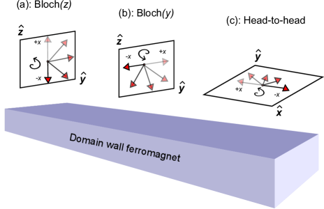
Figure 1: (Color online) Schematic setup: a spin-polarized current is passed through a domain wall magnetic nanowire with spin-orbit coupling. The spin-orbit interaction may be either intrinsic or induced via a heavy metal proximate host. We consider several types of domain wall configurations, since the presence of spin-orbit coupling qualitatively distinguishes the domain wall motion with one type of magnetization texture from another. More specifically, we consider two types of Bloch-domain walls relevant for perpendicular magnetic anisotropy systems in addition to a head-to-head domain wall with an in-plane magnetization easy anisotropy.

Currently, the topic of controllable domain wall motion is receiving much attention (see e.g. Ref. grollier_phys_11, for a very recent review) due to its potential with regard to the storage and transfer of information. A domain wall is a topological defect in a magnetic system where the local magnetic order parameter typically rotates spatially in a fashion that reduces the net magnetic moment of the domain wall area. Owing to their small size ($\sim$ 10 nm) and large velocities ($\sim$ 100 m/s) hayashi_prl_07 ; pizzini_ape_09 , controllable domain wall motion represents holds real potential for tailoring functional devices with fast writing speeds. In addition, there has been several proposals kent_apl_04 ; matsunaga_ape_08 ; parkin_science_08 ; liu_apl_10 related to magnetic memory functionality due to the non-volatile nature of magnetic domains. Walker breakdown walker is nevertheless a limiting factor in this regard.

Domain walls can come in several different shapes depending on the anisotropy energies and dimensionality of the system at hand. In a low-dimensional system such as a magnetic nanowire, Bloch walls are one of the most frequent types encountered. However, it is also possible to generate other sorts of magnetization textures such as head-to-head domain walls. Both of these wall types are shown in Fig. 1. A key question is whether or not specific domain wall types are beneficial with regard to the objectives mentioned above (e.g. fast propagation, low current densities to generate motion). The answer to this question depends on if the spin and position degrees of freedom are correlated in the system, for instance via spin-orbit interaction. In the absence of such spin-orbit interactions, different types of domain walls behave in the same way - the exact magnetization texture has no effect and one obtains for instance the same terminal domain wall velocity in all cases. The fact changes when spin-orbit coupling is present since the electron transport and spin torque now directly depends on the precise magnetization texture, which warrants a specific study for how domain wall motion is manifested for different types of domain walls. A numerical investigation of this issue was recently put forth in Ref. fert_arxiv_12, .

The influence of spin-orbit coupling on domain wall motion has recently been considered extensively in several theoretical works obata_prb_08 ; manchon_prb_09 ; haney_prl_10 ; ryu_jmm_12 ; kim_prb_12 ; linder_prb_13 ; fert_arxiv_12 ; bijl_arxiv_12 . On the experimental stage chernyshov_naturephys_09 ; moore_apl_09 ; kim_ape_10 ; miron_nature_mat_11 , it has been demonstrated that the presence of spin-orbit coupling indeed influences the domain wall dynamics in a non-trivial way including anomalous behavior such as strongly enhanced domain wall velocities and induced wall motion in the opposite direction of the electron flow. In order to explain these findings, it was shown in Ref. kim_prb_12, that the presence of spin-orbit coupling would generate not only a field-like torque but also a so-called Slonczewski-like torque slon , named such due to its formal resemblence to standard current-induced torques in the absence of spin-orbit coupling. Alternatively, these two types of spin-orbit torques may be characterized as out-of-plane and in-plane components of the total Rashba torque wang_arxiv_11 .

Motivated by this, we will in this paper derive exact analytical expressions for the domain wall velocity and Walker breakdown threshold for several types of domain wall configurations when including both types of spin-orbit torques in order to investigate how the Slonczewski-like torque influences the physics at hand. This way, we expand previous literature obata_prb_08 which has only considered the field-like term and show that the inclusion of the Slonczewski-like torque has profound impact on the domain wall velocity and the threshold value of Walker breakdown. In fact, we will show that the existence of this torque renders the threshold value to be universal in the sense that it is independent on both the Gilbert damping $\alpha$, the non-adiabiticity parameter $\beta$, and the chirality $\sigma$ of the domain wall.

We will present a detailed derivation of the equations of motion where possible and show precisely in which manner the spin-orbit coupling influences both the domain wall velocity and the Walker breakdown threshold value. Our analytical expressions show the precise conditions required to realize domain wall motion against the current flow, as has been experimentally observed recently miron_nature_mat_11 , and in particular how the domain wall chirality affects this phenomenon.

Finally, we investigate how the ferromagnetic resonance response of a material (or equivalently the dissipation and pumping of energy) is altered due to the above mentioned spin-orbit torques. The ferromagnetic resonance experiment is an important technique for obtaining information about anisotropy, magnetic damping and magnetization reversal fmr1 ; fmr2 ; fmr3 ; fmr4 ; chen1 ; chen2 ; hasty . The influence of spin-polarized current on Gilbert damping and ferromagnetic resonance have been extensively investigated in different situations fmr5 ; fmr6 ; fmr7 ; fmr8 ; fmr9 ; landeros_prb_08 ; landeros_prb_10 .

Considering a ferromagnetic resonance setup in the presence of a current bias, we analytically show that the spin-orbit interactions render the resonance frequency to become asymmetric with respect to the direction of current injection. This is different from previous works considering a ferromagnetic resonance setup in the presence of spin-transfer torques, albeit without spin-orbit coupling, where the frequency was found to be symmetric with respect to the current direction landeros_prb_10 ; fmr9 .

This paper is organized as follows. In Sec. II, we outline the theoretical framework to be used in our analysis, namely the Landau-Lifshitz-Gilbert (LLG) equation augmented to include the role of spin-orbit coupling combined with a collective-coordinate description of the domain wall. We then present our main findings in Sec. III, in four subsections, where the LLG equation is solved in order to obtain both the domain wall velocity, the Walker breakdown threshold and the ferromagnetic resonance frequency. In Subsec. III.1 we consider Block($z$) wall profile, in Subsec III.2 Block($z$) wall profile is studied, in Subsec. III.3 a head-to-head domain wall structure is investigated, and in Subsec. III.4 we present and discuss the results of absorbed power by a ferromagnetic film under current injection in the presence of Slonczewski-like spin-orbit interaction. We finally summarize our results and findings in Sec. IV.

II Theory

The starting point of our analysis is the spatio-temporal Landau-Lifshitz-Gilbert equation llg , augmented to include the contribution from torque terms arising due to the presence of spin-orbit coupling. When a current-bias is applied along $x$ axis, the full LLG equation takes the form thiaville_epl_05 ; kim_prb_12

$$\partial_{t}\bm{M} =-\gamma\bm{M}\times(\bm{H}_{\text{eff}}+\bm{H}^{so}-\frac{\beta}{M_{0}}\bm{M}\times\bm{H}^{so})$$ (1)

$$+\frac{\alpha}{M_{0}}\bm{M}\times\partial_{t}\bm{M}+\Gamma\partial_{x}\bm{M}-\frac{\beta\Gamma}{M_{0}}\bm{M}\times\partial_{x}\bm{M}.$$

The above equation describes the time-dynamics of the local magnetic order parameter $\bm{M}(x,t)$. The effective field $\bm{H}_{\text{eff}}$ is formally obtained by a functional derivative of the free energy with respect to the magnetization and will vary depending on e.g. the anisotropy configuration of the wire tatara_physrep_08 . The influence of spin-orbit interaction is captured as an effective field:

$$\bm{H}^{so}=\frac{\alpha_{R}m_{e}S}{\hbar eM_{0}(1+\beta^{2})}\hat{\bm{z}}\times\bm{j},$$ (2)

where inversion symmetry is broken in the $z$ direction and $\alpha_{R}$ characterizes the strength of the spin-orbit coupling. $S$ and $j$ is the polarization and density of the injected current, whereas $m_{e}$ and $M_{0}$ is the electron mass and magnitude of the magnetization, respectively. The parameter $\beta$ is known as the non-adiabaticity parameter in the literature, a convention we shall stick to although this terminology is not ideal xiao_prb_06 .

The terms in Eq. (1) have the following physical interpretation. The effective field causes a precession of the magnetization vector $\bm{M}$ and has two extra contributions in terms of $\bm{H}^{so}$ and $\bm{M}\times\bm{H}^{so}$ in the presence of spin-orbit coupling. The former of these has the exact form of an effective field-like torque whereas the latter has the form of a Slonczewksi-like torque. Interestingly, this term was conjectured to exist in the experiment of Miron et al. miron_nature_mat_11 in order to explain the results, but it was only recently theoretically derived in Refs. kim_prb_12, , wang_arxiv_11, . A key observation is that the Slonczewski like spin-orbit torque depends on the non-adiabaticity parameter $\beta$ which also appears for the conventional non-adiabatic spin-transfer torque [last term in Eq. (1)] as is well-known. The term $\propto\partial_{x}\bm{M}$ is the adiabatic spin-transfer torque originating from the assumption that the spin of the conduction electrons follow the domain wall profile perfectly without any loss or spin scattering and $\Gamma=\mu_{B}P/eM_{0}(1+\beta^{2})$.

One of the main goal in this work is to compute the domain wall velocity and analyze Walker breakdown for a domain wall nanowire with spin-orbit coupling, considering several types of experimentally relevant domain walls, both with in-plane and perpendicular magnetization relative the extension of the wire moore_apl_09 ; kim_ape_10 ; miron_nature_mat_11 ; fert_arxiv_12 . We will take into account both the field-like and the Slonczewski-like spin-orbit induced torques. We underline again that the various magnetization textures considered in this paper will give qualitatively different behavior for the wall velocity and Walker threshold values precisely due to the spin-orbit interaction which correlates spin- and real-space. For a Bloch($y$) domain wall (see Fig. 1), an exact analytical solution for the domain wall velocity $v_{\text{DW}}$ is permissible and we will derive this result in detail. For other types of domain walls, a general expression for $v_{\text{DW}}$ is not possible to obtain analytically, thus for completeness, we revert to a numerical study for these cases. However, it is still possible to investigate analytically the Walker breakdown threshold for these domain walls and we show that the chirality of the domain wall conspires with the presence of spin-orbit coupling to qualitatively alter the behavior of Walker breakdown in spin-orbit coupled nanowires.

III Results and Discussion

We shall start by investigating domain wall motion in the presence of multiple spin-orbit torques and consider three types of domain wall structures as shown in Fig. 1. For each case, we will focus on the domain wall velocity and the Walker breakdown threshold value, giving exact analytical results where possible. We note that such an exact solution for $v_{\text{DW}}$ constitutes the most general analytical expression for the domain wall velocity up to now, including fully the influence of spin-orbit coupling. We then study the ferromagnetic resonance response of a magnetic layer with a Slonczewski-like spin-orbit interaction with an injected current into the plane of the layer and using the absorbed power by the film, we drive the ferromagnetic resonance expression analytically.

III.1 Bloch($z$) wall

Consider first a domain wall profile relevant for magnetic nanowires with perpendicular anisotropy moore_apl_09 ; kim_ape_10 ; miron_nature_mat_11 (e.g. Co/Ni multilayers), namely a so-called Bloch($z$) wall which is parametrized as:

$$\bm{m}=(\sin\theta\sin\phi,\sin\theta\cos\phi,\sigma\cos\theta),$$ (3)

and a corresponding effective field:

$$\bm{H}_{\text{eff}} =\frac{2A_{\text{ex}}}{M_{0}^{2}}\nabla^{2}\bm{m}-H_{\perp}m_{x}\hat{x}+H_{k}m_{z}\hat{z}+\bm{H}_{\text{ext}}.$$ (4)

Here, $H_{\perp}$ and $H_{k}$ are the anisotropy fields along the hard and easy axes of magnetization, respectively, whereas $\bm{H}_{\text{ext}}$ is an externally applied magnetic field. The parameter $\sigma=\pm 1$ characterizes the chirality of the domain wall: both signs of $\sigma$ give allowed equilibrium solutions $(\phi=0)$ of the LLG-equation and describes a spin texture changing from positive to negative depending on which direction one is moving in. Note that $\sigma$ is also denoted the topological charge of the domain wall tatara_physrep_08 : the winding direction of the local magnetization dictates the effective ”charge” since the sign of $\sigma$ will determine the direction in which an external magnetic field moves the domain wall. The components of the magnetization vector depend on both space and time according to walker

$$\cos\theta=\tanh\Big{(}\frac{x-X(t)}{\lambda}\Big{)},$$

$$\sin\theta=\text{sech}\Big{(}\frac{x-X(t)}{\lambda}\Big{)}.$$ (5)

Eq. (III.1) is obtained by inserting the magnetization profile $\bm{m}$ into the LLG equation and solving for $\theta$ and $\phi$ under equilibrium conditions (in which case $X(t)$ is a constant and $\phi=0$). The tilt angle $\phi=\phi(t)$ is in general, however, time-dependent and causes the domain wall to acquire a finite component along the hard magnetization axis in an non-equilibrium situation. A collective-coordinate description of the domain wall motion is obtained if one may identify the time-dependence of the domain-wall center position $X(t)$ and the tilt angle $\phi(t)$. In general, other modes of deformation can be allowed tatara_physrep_08 . However, it can be shown that the domain wall may be treated as rigid [only depending on $X(t)$ and $\phi(t)$] in a collective-coordinate framework when the easy axis anisotropy energy $K$ is assumed larger than its hard axis equivalent $K_{\perp}$ tatara_jpsj_08 , i.e. $|K|\gg|K_{\perp}|$.

It is useful to write down an explicitly normalized form of the LLG-equation which we will use for all the domain wall profiles considered in this work. We normalize all quantities to a dimensionless form as defined by the following LLG equation:

$$\partial_{\tau}\bm{m} =-\bm{m}\times(\bm{\mathcal{H}}_{\text{eff}}+\bm{\mathcal{H}}^{so}-\beta\bm{m}\times\bm{\mathcal{H}}^{so})$$

$$+\alpha\bm{m}\times\partial_{\tau}\bm{m}+u\partial_{\tilde{x}}\bm{m}-\beta u\bm{m}\times\partial_{\tilde{x}}\bm{m}.$$ (6)

In the specific case of a Bloch($z$) wall, we then have the normalized effective field:

$$\bm{\mathcal{H}}_{\text{eff}} =2\mathcal{A}\tilde{\nabla}^{2}\bm{m}-\mathcal{H}_{\perp}m_{x}\hat{x}+\mathcal{H}_{k}m_{z}\hat{z},$$

$$\bm{\mathcal{H}}^{so} =\tilde{\alpha}_{R}u\hat{y}.$$ (7)

Inserting Eq. (III.1) into Eq. (III.1) leads to one pair of equations of motion for the collective coordinates $X$ and $\phi$. These equations may be simplified by using Thiele’s approach thiele where one integrates over $x$ and utilizes $\int^{\infty}_{-\infty}\sin^{2}\theta\text{d}x=2\lambda$ and $\int^{\infty}_{-\infty}\sin\theta\text{d}x=\lambda\pi$. We then find the following dimensionless equations:

$$\left\{\begin{array}[]{c}\alpha\partial_{\tau}\phi-\sigma\partial_{\tau}\mathcal{X}=\sigma u-\frac{1}{2}\mathcal{H}_{\perp}\sin 2\phi-\frac{1}{2}\tilde{\alpha}_{R}\pi u\sin\phi,\\ \partial_{\tau}\phi+\alpha\sigma\partial_{\tau}\mathcal{X}=\frac{1}{2}\beta\tilde{\alpha}_{R}u\pi\sin\phi-\beta u\sigma\end{array}\right..$$

Here, $\mathcal{X}=X/\lambda$ is the normalized spatial coordinate of the domain-wall center and $\tilde{\alpha}_{R}$ is a dimensionless measure of the strength of the spin-orbit interaction. In the limiting case of an absent Slonczewski-like spin-orbit torque where the terms proportional to $\beta\times\tilde{\alpha}_{R}$ are zero, our results are consistent with Ref. ryu_jmm_12, . The $\sin\phi$ terms in Eq. (III.1) makes an exact analytical solution of the equations untractable. As we shall see, a similar situation occurs for the head-to-head domain wall case. Nevertheless, it is possible to make further progress in the present case with regard to the appearance of so-called Walker breakdown walker . This phenomenon refers to a threshold value of the current density for which the domain wall starts to rotate with a time-dependent $\phi=\phi(\tau)$ rather than simply propagating with a fixed magnetization texture, i.e. constant $\phi$. In general, it is desirable with as large threshold value as possible for Walker breakdown. We note in passing here that the presence of pinning potentials and defects in the sample may also contribute to the threshold value of the current, but we leave this issue for a future work.

To investigate the velocity at which breakdown occurs, we combine the equations of motion into a single equation for the tilt angle $\phi$:

$$\partial_{\tau}\phi =\frac{1}{1+\alpha^{2}}\Big{[}\frac{1}{2}(\beta-\alpha)\tilde{\alpha}_{R}u\pi\sin\phi-\sigma u(\beta-\alpha)$$

$$-\frac{1}{2}\alpha\mathcal{H}_{\perp}\sin 2\phi\Big{]}.$$ (8)

There is no Walker breakdown as long as $\partial_{\tau}\phi=0$, which holds when the tilt angle $\phi$ satisfies the equation:

$$\sin 2\phi=\frac{(\beta-\alpha)u}{\alpha\mathcal{H}_{\perp}}(\tilde{\alpha}_{R}\pi\sin\phi-2\sigma).$$ (9)

Walker breakdown will occur at a velocity $u_{c}$ such that for $u>u_{c}$ there is no stable solution for this equation. Now, for $|\tilde{\alpha}_{R}\pi|<2$ the right hand side of Eq. (9) will have equal sign for its minimum and maximum value as $\phi$ varies from 0 to $2\pi$. Therefore, Walker breakdown will always occur by increasing $u$: at some value $u_{c}$, the minimum value of the right hand side of Eq. (9) will be larger than unity and thus render the equation to be void of any solution. However, if $|\tilde{\alpha}_{R}\pi|>2$, the minimum and maximum value of the right hand side have opposite signs. This means that there must be a crossing of the 0 line at some values of $\phi$, and thus an intersection with $\sin 2\phi$. In effect, we can always find a stable solution and there will be no Walker breakdown regardless of the velocity $u$ when:

$$\Big{|}\frac{\tilde{\alpha}_{R}\pi}{2}\Big{|}>1.$$ (10)

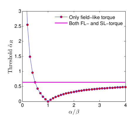
Figure 2: (Color online) Threshold value for the magnitude of the spin-orbit coupling above which there is no Walker breakdown. In the more general scenario where both types of spin-orbit torques are accounted for, the threshold value for $\tilde{\alpha}_{R}$ is constant. When only the field-like torque is considered, the threshold is strongly increased in the regime $\alpha/\beta<0.5$. In the limit $\alpha/\beta\to\infty$, the asymptote is $2/\pi$.

In other words, for a sufficiently large spin-orbit interaction, no Walker breakdown occurs. It is interesting to note that this condition is universal in the sense that it is independent on the damping parameter $\alpha$, the non-adiabiticity parameter $\beta$, and the chirality $\sigma$ of the domain wall. This observation can be attributed directly to the presence of the new spin-orbit torque proportional to $\beta$. To see this, consider a scenario where only the field-like spin-orbit torque $\propto\bm{M}\times\bm{H}_{so}$ is included. All terms proportional to $\beta\times\tilde{\alpha}_{R}$ are then zero, and we obtain the equation

$$\sin 2\phi=\frac{2\sigma u}{\mathcal{H}_{\perp}}\Big{(}1-\beta/\alpha-\frac{\sigma\tilde{\alpha}_{R}\pi}{2}\sin\phi\big{)},$$ (11)

which must be satisfied to prevent Walker breakdown. As seen, whether or not the maximum and minimum value of the right hand side have equal sign depends on if

$$\Big{|}\frac{\tilde{\alpha}_{R}\pi}{2}\Big{|}>|(1-\beta/\alpha)|.$$ (12)

In this regime, we recover the results of Ref. ryu_jmm_12, . The effect of the Slonczewski-like spin-orbit torque is then to render the Walker breakdown universal (independent on $\alpha,\beta,\sigma$). Let us also consider the implications this torque-term has with regard to the magnitude of the threshold value for Walker breakdown. Comparing Eqs. (10) and (12), we see that the required spin-orbit interaction $\tilde{\alpha}_{R}$ to completely remove the Walker threshold depends on the ratio $\beta/\alpha$ if one does not take into account the Slonczewski-like spin-orbit torque. For $\beta/\alpha\simeq 1$, the required spin-orbit strength becomes very small. In the more general case where the aforementioned torque is included, however, the required $\tilde{\alpha}_{R}$ has a fixed value. This is shown in Fig. 2.

We also give numerical results for the wall velocity for this Bloch domain wall configuration, using a similar approach as in Ref. linder_prb_11, . Let us first note that it is possible to infer what the qualitative effect is of the chirality $\sigma$ directly from the equations of motion Eqs. (III.1). By making the transformation $\phi\to\sigma\phi$, it is seen that the equations of motion become independent on the chirality $\sigma.$ This means that the domain wall velocity will be the same regardless of the sign of $\sigma$, whereas the tilt angle $\phi$ evolves in the opposite direction with time for opposite signs of $\sigma$. In Fig. 3, we therefore present results for $\sigma=1$ without loss of generality and consider two cases with damping $\alpha$ larger or smaller than the non-adiabaticity constant $\beta$ in (a) and (b), respectively. As seen, this qualitatively affects the domain wall velocity.

A particular feature worth noting in (b) is that the abrupt change in wall velocity at a given $u$ is not necessarily synonymous with the occurrence of Walker breakdown. To see this, consider Fig. 4 where we have plotted the left- and right-hand side of the Walker breakdown criterion Eq. (9) in addition to the time-evolution of the tilt angle $\phi$ as an inset. We have set $\alpha=0.005$ and $\beta=0.01$ and consider two strengths of the spin-orbit coupling parameter $\tilde{\alpha}_{R}$ in (a) and (b). An intersection of the lines in the main panels means that there exists a solution to Eq. (9) and that Walker breakdown does not occur. Considering Fig. 4(a) first, we see that increasing the current density eventually causes Walker breakdown as the dashed and full lines no longer intersect. As a result, $\phi$ is no longer a constant as seen in the inset and starts to grow with time. We may therefore conclude that the abrupt change in wall velocity for $\tilde{\alpha}_{R}=0.01$ seen in Fig. 3(b) does correspond to the occurrence of Walker breakdown. However, turning to Fig. 4(b) it is seen that the dashed and full lines always intersect even when increasing the current density $u$ above the value at which the wall velocity abruptly changes in Fig. 3(b) for $\tilde{\alpha}_{R}=1$ (around $u=0.14$). What is important to note is that their point of intersection changes discontinuously: the tilt angle $\phi$ remains constant so that there is no Walker breakdown in the sense of a continuously deforming domain wall. Instead, there is an abrupt change in the tilt angle where it changes from one constant value to another.

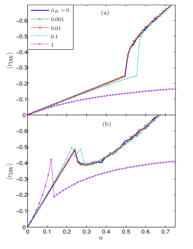
Figure 3: (Color online) Domain wall velocity for a Bloch($z$) wall plotted against the injected current. We have chosen $\sigma=1$ without loss of generality (see text) and set $\beta=0.01$ and $\mathcal{H}_{\perp}$=0.5. In (a) $\alpha>\beta$ ($\alpha=0.02$) whereas in (b) $\alpha<\beta$ ($\alpha=0.005$). Note the inverted sign of the $y$ axis, which simply corresponds to the direction of the wall motion.

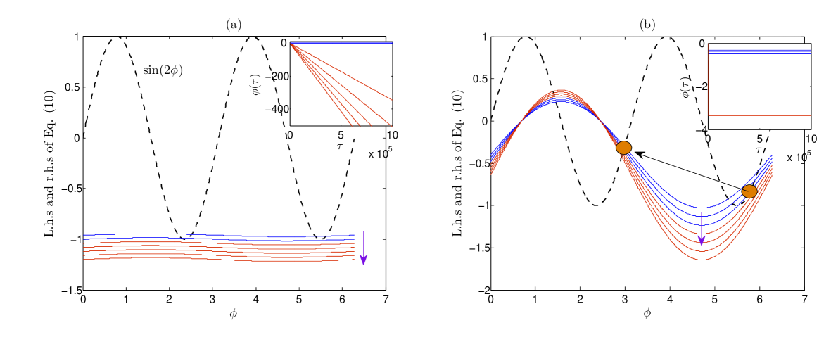
Figure 4: (Color online) Plot of left-hand side (dashed line) and right-hand side (full lines) of Eq. (9) in order to illustrate the intersection points. When there is no intersection between the lines, Walker breakdown has occurred. We have set $\beta=0.01$, $\alpha=0.005$ and consider (a) $\tilde{\alpha}_{R}=0.01$ and $u$ ranging from 0.24 to 0.30 along the direction of the arrow, in addition to (b) $\tilde{\alpha}_{R}=1$ and $u$ ranging from 0.10 to 0.16 along the direction of the arrow. The black arrow between the circles in (b) highlights how the intersection point changes abruptly upon increasing $u$. Insets: Time-evolution of the tilt angle for the same choices of $u$.

III.2 Bloch($y$) wall

Another type of domain wall structure which may appear in such a systems with perpendicular magnetic anisotropy is the Bloch$(y)$-wall, having the easy magnetization direction along the $y$ axis whereas the hard axis remains along the wire direction:

$$\bm{m}=(\sin\theta\sin\phi,\sigma\cos\theta,\sin\theta\cos\phi),$$ (13)

and a corresponding effective field:

$$\bm{H}_{\text{eff}} =\frac{2A_{\text{ex}}}{M_{0}^{2}}\nabla^{2}\bm{m}-H_{\perp}m_{x}\hat{x}+H_{k}m_{y}\hat{y}+\bm{H}_{\text{ext}}.$$ (14)

In this case, the equations of motion for the collective coordinates $\mathcal{X}$ and $\phi$ take a different form compared to the Bloch($z$) case:

$$\left\{\begin{array}[]{c}\sigma\partial_{\tau}\mathcal{X}+\alpha\partial_{\tau}\phi=\beta\tilde{\alpha}_{R}u-\frac{1}{2}\mathcal{H}_{\perp}\sin 2\phi-u\sigma,\\ \partial_{\tau}\phi-\alpha\sigma\partial_{\tau}\mathcal{X}=\beta u\sigma+\tilde{\alpha}_{R}u\end{array}\right..$$

In fact, these equations can now be solved analytically in an exact manner, using a similar approach as in Ref. linder_prb_13, . Combining the two above equations yields:

$$\partial_{\tau}\phi(1+\alpha^{2})=-\frac{\alpha}{2}\mathcal{H}_{\perp}\sin 2\phi+u[\sigma(\beta-\alpha)+\tilde{\alpha}_{R}(1+\alpha\beta)].$$ (15)

Consider Eq. (15) with respect to $\phi=\phi(\tau)$. This is a separable equation and direct integration gives:

$$\tau =\mathcal{C}_{0}-\frac{1+\alpha^{2}}{\sqrt{\mathcal{A}^{2}-\alpha^{2}\mathcal{H}_{\perp}^{2}/4}}\text{atan}\Big{[}\frac{\alpha\mathcal{H}_{\perp}/2-\mathcal{A}\tan\phi}{\sqrt{\mathcal{A}^{2}-\alpha^{2}\mathcal{H}_{\perp}^{2}/4}}\Big{]},$$ (16)

where $\mathcal{C}_{0}$ is an integration constant and we define:

$$\mathcal{A}\equiv u[\sigma(\beta-\alpha)+\tilde{\alpha}_{R}(1+\alpha\beta)].$$ (17)

For brevity of notation, we also introduce $\mathcal{B}\equiv\alpha\mathcal{H}_{\perp}/2$. The integration constant depends on the initial conditions. At $\tau=0$, we assume that the domain wall is in its equilibrium configuration $\phi=0$, in which case we may write the solution for the tilt angle as:

$$\tan\phi =\frac{\mathcal{B}}{\mathcal{A}}-\frac{\sqrt{\mathcal{A}^{2}-\mathcal{B}^{2}}}{\mathcal{A}}\tan\Big{[}\text{atan}(\alpha\mathcal{B}/\sqrt{\mathcal{A}^{2}-\mathcal{B}^{2}})$$

$$-\tau\sqrt{\mathcal{A}^{2}-\mathcal{B}^{2}}/(1+\alpha^{2})\Big{]}.$$ (18)

Having now obtained the full time-dependence of the tilt-angle, we insert this back into the original equation of motion in order to find the domain wall velocity $\dot{\mathcal{X}}=v_{\text{DW}}$. The general expression for the domain wall velocity is rather large. However, by utilizing the fact that $v_{\text{DW}}$ will display small-scale oscillations it is possible to find a simplified expression for the average domain wall velocity $\langle v_{\text{DW}}\rangle$. The period of oscillation is $T=(1+\alpha^{2})\pi/\sqrt{\mathcal{A}^{2}-\mathcal{B}^{2}}$, which gives us:

$$\langle v_{\text{DW}}\rangle =\frac{1}{T}\int^{T}_{0}\text{d}\tau\frac{\sigma}{\alpha}\Bigg{\{}\frac{\mathcal{A}^{2}-\mathcal{B}^{2}}{\mathcal{A}(1+\alpha^{2})}\text{sec}^{2}\Big{(}\text{atan}(\alpha\mathcal{B}/\sqrt{\mathcal{A}^{2}-\mathcal{B}^{2}})-\tau\frac{\sqrt{\mathcal{A}^{2}-\mathcal{B}^{2}}}{1+\alpha^{2}}\Big{)}$$

$$\times\Big{[}1+\Big{(}\frac{\alpha\mathcal{B}}{\mathcal{A}}-\sqrt{\mathcal{A}^{2}-\mathcal{B}^{2}}{\mathcal{A}}\tan[\text{atan}(\alpha\mathcal{B}/\sqrt{\mathcal{A}^{2}-\mathcal{B}^{2}})-\tau\sqrt{\mathcal{A}^{2}-\mathcal{B}^{2}}/(1+\alpha^{2})]\Big{)}^{2}\Big{]}^{-1}\Bigg{\}}-u(\tilde{\alpha}_{R}\sigma+\beta)/\alpha.$$ (19)

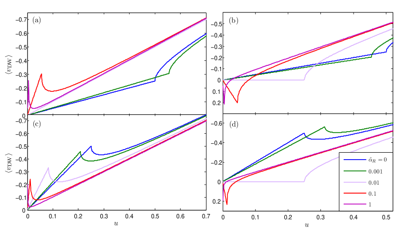
Figure 5: (Color online) The domain wall velocity $\langle v_{\text{DW}}\rangle$ as a function of the current density $u$ for various chiralities and spin-orbit coupling strengths. (a): Positive chirality $\sigma=+1$ and $\alpha>\beta$ ($\alpha=0.02$). (b): Negative chirality $\sigma=-1$ and $\alpha>\beta$ ($\alpha=0.02$). (c): Positive chirality $\sigma=+1$ and $\alpha<\beta$ ($\alpha=0.005$). (d): Negative chirality $\sigma=-1$ and $\alpha<\beta$ ($\alpha=0.005$). For all plots, we have used $\beta=0.01$ and $\mathcal{H}_{\perp}=0.5$.

The analytical solution to the above integral and the final result is:

$$\langle v_{\text{DW}}\rangle =\frac{\sigma}{\alpha(1+\alpha^{2})}\text{sgn}\{u\sigma(\beta-\alpha)+u\tilde{\alpha}_{R}(1+\alpha\beta)\}\times\text{Re}\sqrt{[u\sigma(\beta-\alpha)+u\tilde{\alpha}_{R}(1+\alpha\beta)]^{2}-\alpha^{2}\mathcal{H}_{\perp}^{2}/4}-u(\tilde{\alpha}_{R}\sigma+\beta)/\alpha,$$ (20)

where we have reinstated the original parameters contained in the quantities $\mathcal{A}$ and $\mathcal{B}$. The equation for $\langle v_{\text{DW}}\rangle$ shows the exact manner in which the domain wall velocity depends on the various torque terms such as the non-adiabatic contribution $\beta$ and the spin-orbit terms $\tilde{\alpha}_{R}$, and reveals several important features. It is seen that for this particular domain wall configuration [Bloch$(y)$], the effect of the Slonczewski-like spin-orbit torque is a small quantitative correction of order $\mathcal{O}(\alpha\beta)$, which thus can be neglected. However, the conventional field-like spin-orbit torque has a strong qualitative influence on the wall dynamics. In fact, it is seen that the $\tilde{\alpha}_{R}$ term plays the same role as the non-adiabatic conventional torque proportional to $\beta$, but with one important difference: the spin-orbit torque contribution is chirality dependent, i.e. changes sign with $\sigma$, whereas the $\beta$-term does not. As a consequence, the wall may actually propagate in opposite direction of the applied current depending on the chirality $\sigma$ of the domain wall, as was shown recently in Ref. linder_prb_13, .

It is seen from Eq. (20) that there is either an enhancement of the domain wall velocity or a competition between the spin-orbit induced torque and $\beta$-torque depending on the sign of $\sigma$. We show this in Fig. 5 where we consider the four possible combinations of wall chirality $\sigma$ (two values, $\sigma=\pm 1$) combined with whether or not $\alpha$ is larger than $\beta$ (two possibilities, $\alpha>\beta$ or $\alpha<\beta$). For a positive chirality $\sigma=+1$ displayed in Fig. 5 (a) and (c), the wall moves in the same direction for all current densities $u$ as the torque terms in Eq. (20) have the same sign. This is no longer the case for the opposite chirality $\sigma=-1$ shown in Fig. 5(b) and (d) where the wall velocity can actually change sign as $u$ increases. This is indicative of counterflow domain wall motion where the wall moves in the opposite direction of the applied spin current.

Walker breakdown for the domain wall occurs for velocities $u\geq u_{c}$ where the root in Eq. (20) becomes imaginary, namely:

$$u_{c}=\frac{\alpha\mathcal{H}_{\perp}}{|2\sigma(\beta-\alpha)+2\tilde{\alpha}_{R}(1+\alpha\beta)|}.$$ (21)

Note that this is the same as $u_{c}$ that we would have found using the arguments in the previous section in order to identify the Walker breakdown from the equations of motion (without actually solving them explicitly) and thus serves as a consistency check for the correctness of Eq. (20). This expression is quite generally valid, including the effects of both types of spin-orbit torques and both types of conventional spin-transfer torques. As another consistency check, we observe that in the absence of spin-orbit coupling ($\tilde{\alpha}_{R}=0$), one finds that $|u_{c}|=\alpha\mathcal{H}_{\perp}/2|\beta-\alpha|$ which agrees with Ref. thiaville_epl_05, . The effect of the spin-orbit interaction is seen to depend explicitly on the chirality $\sigma$ of the domain wall. Although Walker breakdown is inevitable for the present Bloch($y$) domain wall, in contrast to the Bloch($z$) one, the presence of spin-orbit interactions $(\tilde{\alpha}_{R}\neq 0$) can strongly enhance the threshold velocity due to the competition between the terms $\sigma(\beta-\alpha)$ and $\tilde{\alpha}_{R}(1+\alpha\beta)$ in the denominator. When these terms have different sign (either for $\sigma=-1$ and $\beta>\alpha$ or $\sigma=1$ and $\beta<\alpha$), the spin-orbit coupling can very strongly enhance the threshold current for Walker breakdown. This effect could be used to infer information about the value of $\alpha$ and $\beta$ precisely due to the non-monotonic behavior of the threshold current as a function of $\tilde{\alpha}_{R}$.

We illustrate this behavior in Fig. 6 where we have chosen $\sigma=+1$. As seen, the threshold velocity decreases in a monotonic fashion with increasing $\tilde{\alpha}_{R}$ when the damping is low, $\alpha<\beta$. However, when the two terms in the denominator differ in sign (which occurs precisely when $\alpha>\beta$), the threshold velocity $u_{c}$ has a non-monotonic behavior and is in fact strongly increases near $\tilde{\alpha}_{R}=|\beta-\alpha|$. In this way, one may obtain information regarding the relative size of $\alpha$ and $\beta$ by measuring the threshold velocity.

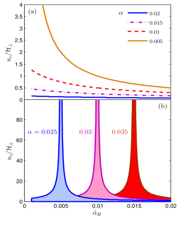
Figure 6: (Color online) Critical velocity $u_{c}/\mathcal{H}_{\perp}$ that triggers Walker breakdown. We have chosen $\beta=0.02$ as a representative value which demonstrates the fundamental behavior of $u_{c}$. For sufficiently low damping $\alpha<\beta$ shown in (a), the threshold velocity is lowered monotonically as the spin-orbit interaction $\tilde{\alpha}_{R}$ is increased. When the damping becomes stronger such that $\alpha>\beta$, $u_{c}$ is strongly enhanced in a limited interval of $\tilde{\alpha}_{R}$.

III.3 Head-to-head domain wall

The final type of domain wall structure we will consider appears for in-plane magnetized strips (e.g. NiFe layer fert_arxiv_12 ) and is known as a so-called head-to-head domain wall. In this case, the easy axis is parallell with the extension of the wire whereas the hard axis is perpendicular to it:

$$\bm{m}=(-\sigma\cos\theta,\sin\theta\cos\phi,\sin\theta\sin\phi),$$ (22)

and a corresponding effective field:

$$\bm{H}_{\text{eff}} =\frac{2A_{\text{ex}}}{M_{0}^{2}}\nabla^{2}\bm{m}-H_{\perp}m_{z}\hat{z}+H_{k}m_{x}\hat{x}+\bm{H}_{\text{ext}}.$$ (23)

Using again Thiele’s approach as described in the previous sections, one arrives at exactly the same equations of motion as in the Bloch($z$) case. The formal reason for this can be traced back to the fact that the effective spin-orbit field $\bm{H}^{so}$ is directed along the $y$ axis. The magnetization textures of the Bloch($z$) and head-to-head domain walls may be transformed into each other via an SO(3) rotation with an angle $\pi/2$ of $\bm{M}$ around the $y$ axis. Such a rotation leaves $\bm{H}^{so}$ invariant and one thus obtains the same equations of motion for both types of domain walls. Formally, one can see this by multiplying Eq. (1) from the left side with:

$$\mathcal{U}=\begin{pmatrix}0&0&-1\\ 0&1&0\\ 1&0&0\\ \end{pmatrix},$$ (24)

and using that

$$(\mathcal{U}\bm{a})\times(\mathcal{U}\bm{b})=\text{det}(\mathcal{U})(\mathcal{U}^{-1})^{\text{T}}(\bm{a}\times\bm{b}).$$ (25)

Since $\mathcal{U}\in$ SO(3), we have that $(\mathcal{U}^{-1})^{\text{T}}=\mathcal{U}$ and det$(\mathcal{U})$=+1. By direct multiplication, one observes that $\mathcal{U}\bm{H}^{so}=\bm{H}^{so}$, $\mathcal{U}\bm{M}_{\text{Bloch$(z)$}}=\bm{M}_{\text{head-to-head}}$ and $\mathcal{U}\bm{H}^{\text{eff}}_{\text{Bloch$(z)$}}=\bm{H}^{\text{eff}}_{\text{head-to-head}}$. Note that it is in drastic contrast with the Bloch($y$) case where $\bm{H}^{so}$ is not invariant under the matrix which rotates $\bm{M}_{\text{Bloch$(z)$}}$ into $\bm{M}_{\text{Bloch$(y)$}}$. The same arguments and results related to the domain wall velocity and Walker breakdown that were discussed in Sec. III.1 then also hold for the present head-to-head domain wall case.

We mention here that the equivalence of the Bloch($z$) and head-to-head domain wall case found here is contingent on the specific setup we have considered in Fig. 1. Although this model is the standard one and indeed the most frequently employed setup experimentally, it was recently shown that such an equivalence does not hold when combining a magnetic strip/wire with a non-magnetic conductive layer with spin-orbit interaction in a non-parallell geometry fert_arxiv_12 . Such a method actually provides a manner in which the direction of the effective spin-orbit field can be changed which could then serve as a mean to distinguish between different types of domain walls, based on their response to an applied current.

III.4 Ferromagnetic resonance (FMR) in the presence of spin-orbit torques

We now turn our attention to another setup where the aim is to identify the ferromagnetic resonance response of a material where spin-orbit interactions play a prominent role. To do so, we consider the setup shown in Fig. 7 where a spin-current with polarization magnitude and unit vector direction $S\in[0,1]$ and $\vec{\ddot{S}}$, respectively, is injected into the ferromagnetic layer where spin-orbit coupling is present. This directly influences the susceptibility tensor and thus both the ferromagnetic resonance frequency/linewidth and the absorbed power by the system prb_86_dreher .

To facilitate the analytical calculations, we will operate with two different coordinate systems. The laboratory (stationary) framework $\ddot{x}\ddot{y}\ddot{z}$ is shown in Fig. 7, where the $\ddot{x}\ddot{y}$ plane spans the ferromagnetic layer, and $xyz$ denotes a rotated coordinate system which we will specify the direction and purpose of below. A current is injected into the ferromagnetic layer acting with a spin-transfer torque on the magnetization vector $\vec{\ddot{\mathcal{M}}}$. This torque is modified due to the presence of spin-orbit coupling which is taken into account via a field $\vec{\ddot{H}}^{so}$ as in the domain-wall treatment. The time-dependent LLG motion equation describing the dynamic of ferromagnetic layer magnetization vector then takes the following form in this new notation:

$$\frac{\partial\vec{\ddot{\mathcal{M}}}}{\partial t}=-\gamma\vec{\ddot{\mathcal{M}}}\times\vec{\ddot{H}}^{t}+\frac{\alpha}{\ddot{\mathcal{M}}_{S}}\vec{\ddot{\mathcal{M}}}\times\frac{\partial\vec{\ddot{\mathcal{M}}}}{\partial t}$$

$$+\frac{\gamma}{\ddot{\mathcal{M}}_{S}}\vec{\ddot{\mathcal{M}}}\times\vec{\ddot{\mathcal{M}}}\times(\beta\vec{\ddot{H}}^{so}+P_{s}\vec{\ddot{S}}),$$ (26)

$$\vec{\ddot{H}}^{so}=\frac{\alpha_{R}m_{e}S}{\hbar e\mathcal{\ddot{M}}_{S}(1+\beta^{2})}(\vec{\ddot{n}}\times\vec{\ddot{J}}_{e}),\;\;P_{s}=\frac{\hbar SJ_{e}}{2e\mathcal{\ddot{M}}_{S}d}.$$

Here, $\gamma$ is the electron gyromagnetic ratio and $\alpha$ is the Gilbert damping constant. Moreover, $\beta$ is the non-adiabaticity parameter discussed previously, $P_{s}$ is the spin-torque parameter, $S$ is the polarization of injected current into the ferromagnetic layer, and a normal vector to the plane of ferromagnetic layer is represented by $\vec{\ddot{n}}$ (see Fig. 7).

We now introduce a rotated coordinate system $xyz$ where the saturation magnetization direction is parallel with the $z$ axis. The orientation of the rotated system $xyz$ compared to the stationary one $\ddot{x}\ddot{y}\ddot{z}$ is determined by calculating the equilibrium orientation of the magnetization order parameter and setting the $z$ axis to be parallel with it. The details of the calculations will be discussed in what follows.

We define a transformation matrix which rotates the fixed coordinate system so that its $z$ axis to be oriented along $\vec{\ddot{\mathcal{M}}}_{S}$. Therefore, all other vector quantities should be rotated via the defined transformation to be described in this new rotated coordinate system. If we describe $\vec{\ddot{\mathcal{M}}}_{S}$ by polar and azimuthal angles i.e. $\theta_{\ddot{M}}$ and $\varphi_{\ddot{M}}$, in the fixed original coordinate system, a rotation around the $\ddot{z}$ axis equal to $\varphi_{\ddot{M}}$ and then around the rotated $\ddot{y}$ axis equal to $\theta_{\ddot{M}}$ are required for aligning $\ddot{z}$ axis and $\vec{\ddot{\mathcal{M}}}_{S}$ orientations. Hence, the rotation matrices can be respectively given by (see Ref. arfken, for more details):

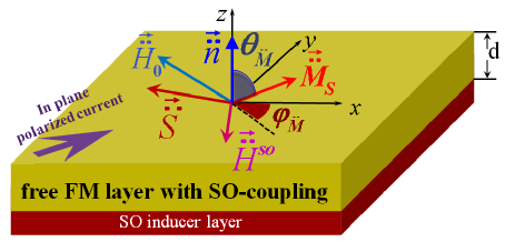
Figure 7: (Color online) Schematic setup of the free ferromagnetic (FM) layer with a general saturation magnetization direction, $\vec{\ddot{\mathcal{M}}}_{S}$, described by polar and azimuthal angles $\theta_{\ddot{M}}$ and $\varphi_{\ddot{M}}$, respectively. The thickness of free ferromagnetic layer is denoted by $d$. The externally applied static magnetic field $\vec{\ddot{H}}_{0}$, polarization vector of injected charge current $\vec{\ddot{S}}$, spin-orbit coupling torque vector $\vec{\ddot{H}}^{so}$, and finally normal unity vector $\vec{\ddot{n}}$ are shown. The ferromagnetic film is located in the $\ddot{x}\ddot{y}$ plane so that $\ddot{z}$ axis is normal to the ferromagnetic film. The spin-orbit coupling is assumed to be induced via a substrate layer into the free ferromagnetic layer. The double dot represents the vector quantities in the non-rotated coordinate system (laboratory framework).

$$R_{z}(-\varphi_{\ddot{M}})=\left(\begin{array}[]{ccc}\cos\varphi_{\ddot{M}}&-\sin\varphi_{\ddot{M}}&0\\ \sin\varphi_{\ddot{M}}&\cos\varphi_{\ddot{M}}&0\\ 0&0&1\end{array}\right),$$ (30)

$$R_{y}(\theta_{\ddot{M}})=\left(\begin{array}[]{ccc}\cos\theta_{\ddot{M}}&0&-\sin\theta_{\ddot{M}}\\ 0&1&0\\ \sin\theta_{\ddot{M}}&0&\cos\theta_{\ddot{M}}\end{array}\right).$$ (34)

The total rotation matrix is thus the multiplication of $R_{y}$ and $R_{z}$ i.e.

$$R^{t}=R_{y}R_{z}=$$

$$\left(\begin{array}[]{ccc}\cos\theta_{\ddot{M}}\cos\varphi_{\ddot{M}}&-\cos\theta_{\ddot{M}}\sin\varphi_{\ddot{M}}&-\sin\theta_{\ddot{M}}\\ \sin\varphi_{\ddot{M}}&\cos\varphi_{\ddot{M}}&0\\ \sin\theta_{\ddot{M}}\cos\varphi_{\ddot{M}}&-\sin\theta_{\ddot{M}}\sin\varphi_{\ddot{M}}&\cos\theta_{\ddot{M}}\end{array}\right).$$ (38)

We characterize each vector quantity by its polar and azimuthal angle in the fixed original coordinate system shown in Fig. 7. Since we assume a homogeneous magnetization texture (macrospin approximation), we have $\vec{\nabla}^{2}\vec{\ddot{\mathcal{M}}}=0$. The total effective field entering the LLG-equation may now be decomposed into the following terms:

$$\vec{H}^{t} =\vec{H}^{dip}+\vec{h}^{dip}(t)+\vec{H}^{a}+\vec{h}^{a}(t)+\vec{H}^{so}$$

$$+b\vec{S}+\vec{H}_{0}+\vec{h}^{ext}(t)$$

$$\equiv\vec{H}+\vec{h}(t).$$ (39)

Above, $\{\vec{H}^{dip},\vec{h}^{\text{dip}}(t)\}$ and $\{\vec{H}^{a},\vec{h}^{a}(t)\}$ are the static and dynamic parts of the dipole and anisotropy fields respectively, $\vec{H}^{so}$ is the spin-orbit field, $b\vec{S}$ is the spin-torque effective field (which is usually negligible), $\vec{H}_{0}$ is the static externally applied field, and finally $\vec{h}^{ext}(t)$ is a small rf field applied perpendicularly to the saturation magnetization direction $z$ in order to probe the ferromagnetic resonance. To show an example of how the quantities in the two coordinate systems are related, note that the $x$, $y$, and $z$ components of the externally applied static magnetic field $\vec{H}_{0}$ in the rotated coordinate system are given by:

$$H_{0x}=\ddot{H}_{0}\left\{\cos\theta_{\ddot{M}}\cos\varphi_{\ddot{M}}\sin\theta_{\ddot{H}_{0}}\cos\varphi_{\ddot{H}_{0}}-\right.$$

$$\left.\cos\theta_{\ddot{M}}\sin\varphi_{\ddot{M}}\sin\theta_{\ddot{H}_{0}}\cos\varphi_{\ddot{H}_{0}}-\sin\theta_{\ddot{M}}\cos\theta_{\ddot{H}_{0}}\right\},$$ (40)

$$H_{0y}=\ddot{H}_{0}\left\{\sin\varphi_{\ddot{M}}\sin\theta_{\ddot{H}_{0}}\cos\varphi_{\ddot{H}_{0}}+\right.$$

$$\left\{\cos\varphi_{\ddot{M}}\sin\theta_{\ddot{H}_{0}}\cos\varphi_{\ddot{H}_{0}}\right\},$$ (41)

$$H_{0z}=\ddot{H}_{0}\left\{\sin\theta_{\ddot{M}}\cos\varphi_{\ddot{M}}\sin\theta_{\ddot{H}_{0}}\cos\varphi_{\ddot{H}_{0}}-\right.$$

$$\left.\sin\theta_{\ddot{M}}\sin\varphi_{\ddot{M}}\sin\theta_{\ddot{H}_{0}}\cos\varphi_{\ddot{H}_{0}}-\cos\theta_{\ddot{M}}\cos\theta_{\ddot{H}_{0}}\right\}.$$ (42)

As mentioned above, the dipole field can be divided into static $\vec{H}^{dip}$ and dynamic $\vec{h}^{dip}(t)$ parts. In the rotated coordinate system they may be obtained as landeros_prb_08 :

$$\vec{H}^{dip}=\mathcal{M}\cos\theta_{\ddot{M}}\left(\begin{array}[]{c}\cos\theta_{\ddot{M}}\sin\varphi_{\ddot{M}}\\ -\cos\varphi_{\ddot{M}}\\ \sin\theta_{\ddot{M}}\sin\varphi_{\ddot{M}}\end{array}\right),$$ (46)

$$\vec{h}^{dip}(t)=4\pi m_{y}(t)\sin\theta_{\ddot{M}}\left(\begin{array}[]{c}\cos\theta_{\ddot{M}}\sin\varphi_{\ddot{M}}\\ -\cos\varphi_{\ddot{M}}\\ \sin\theta_{\ddot{M}}\sin\varphi_{\ddot{M}}\end{array}\right),$$ (50)

where $\mathcal{M}\approx 4\pi\mathcal{M}_{S}-H^{a}$. Assuming a weak rf magnetic field applied transverse to the $\hat{z}$-direction, we may consider the components of magnetization in the rotated coordinate system as $\mathcal{M}_{z}=\mathcal{M}_{S}\gg\mathcal{M}_{x},\mathcal{M}_{y}$. In this case, the following time-dependent coupled differential equations for the precessing magnetization components are obtained;

$$\frac{\partial\mathcal{M}_{x}}{\partial t}=-\gamma\mathcal{M}_{y}H_{z}^{t}+\gamma\mathcal{M}_{x}(\beta H_{z}^{so}+P_{s}S_{z})$$

$$+\gamma\mathcal{M}_{S}(H_{y}^{t}-(\beta H_{x}^{so}+P_{s}S_{x}))-\alpha\frac{\partial\mathcal{M}_{y}}{\partial t},$$

$$\frac{\partial\mathcal{M}_{y}}{\partial t}=\gamma\mathcal{M}_{x}H_{z}^{t}+\gamma\mathcal{M}_{y}(\beta H_{z}^{so}+P_{s}S_{z})$$

$$-\gamma\mathcal{M}_{S}(H_{x}^{t}+(\beta H_{y}^{so}+P_{s}S_{y}))+\alpha\frac{\partial\mathcal{M}_{x}}{\partial t},$$

$$\frac{\partial\mathcal{M}_{z}}{\partial t}=\frac{\partial\mathcal{M}_{S}}{\partial t}=0=\gamma\mathcal{M}_{x}(-H_{y}^{t}+(\beta H_{x}^{so}+P_{s}S_{x}))$$

$$+\gamma\mathcal{M}_{y}(H_{x}^{t}+(\beta H_{y}^{so}+P_{s}S_{y})).$$

Setting the transverse part of the magnetization and fields equal to zero in the above equations for $\partial_{t}\mathcal{M}_{x}$ and $\partial_{t}\mathcal{M}_{y}$, one obtains the equilibrium conditions which specify the orientation of the $z$ axis:

$$\left\{\begin{array}[]{c}H_{x}+(\beta_{so}H_{y}^{so}+\beta_{s}S_{y})=0\\ H_{y}-(\beta_{so}H_{x}^{so}+\beta_{s}S_{x})=0\\ \end{array}\right..$$ (53)

This is consistent with the equation for $\partial_{t}\mathcal{M}_{z}$ and our preassumption namely; $\mathcal{M}_{z}\gg\mathcal{M}_{x},\mathcal{M}_{y}$ . In order to obtain the solution for the transverse components $\mathcal{M}_{x}$ and $\mathcal{M}_{y}$ to lowest order, we now substitute these conditions back into the equations of motion for the magnetization components above and obtain:

$$\frac{\partial\mathcal{M}_{x}}{\partial t} = -\gamma\mathcal{M}_{y}H_{z}+\gamma\mathcal{M}_{S}h_{y}(t)-\alpha\frac{\partial\mathcal{M}_{y}}{\partial t}$$

$$+\gamma\mathcal{M}_{x}(\beta H^{so}_{z}+P_{s}S_{z}),$$

$$\frac{\partial\mathcal{M}_{y}}{\partial t} = +\gamma\mathcal{M}_{x}H_{z}-\gamma\mathcal{M}_{S}h_{x}(t)+\alpha\frac{\partial\mathcal{M}_{x}}{\partial t}$$

$$+\gamma\mathcal{M}_{y}(\beta H^{so}_{z}+P_{s}S_{z}).$$

In our calculations we have set the time-dependent fields sufficienty small so that those terms including higher orders of time-dependent components are negligible. Assuming that the the external time-dependent magnetic field induces the same frequency in all time-dependent components of other vector quantities (including responses) as itself, $\Omega$, we get e.g. $\vec{h}^{dip}(t)=\vec{h}^{dip}e^{-i\Omega t}$. By substituting this time-dependency into Eqs. (III.4) we arrive at $\tilde{\mathcal{M}}(t)=\chi\tilde{h}^{ext}(t)$ in which $\tilde{\mathcal{M}}(t)=(\mathcal{M}_{x},\mathcal{M}_{y})^{T}$, $\tilde{h}^{ext}(t)=(h_{x}^{ext},h_{y}^{ext})^{T}$, and;

$$\chi=\left(\begin{array}[]{cc}\chi_{xx}&\chi_{xy}\\ \chi_{yx}&\chi_{yy}\\ \end{array}\right).$$ (57)

$\chi$ is known as the susceptibility tensor which determines the behavior of magnetization in response to the external time-dependent magnetic field. The components of the obtained susceptibility tensor in the presence of spin-orbit coupling read:

$$\chi_{xx} = +\Gamma\left\{\gamma\mathcal{W}_{y}\Xi-\Delta\alpha\Omega-i(\gamma\Delta\mathcal{W}_{y}+\Omega\alpha\Xi)\right\},$$

$$\chi_{xy} = -\Gamma\left\{\Sigma\Xi+\Delta\Omega-i(\Delta\Sigma-\Omega\Xi)\right\},$$

$$\chi_{yx} = +\Gamma\left\{\Sigma\Xi+\Delta\Omega-i(\Delta\Sigma-\Omega\Xi)\right\}$$

$$\chi_{yy} = +\Gamma\left\{\gamma\mathcal{W}_{x}\Xi-\Delta\alpha\Omega-i(\gamma\Delta\mathcal{W}_{x}+\Omega\alpha\Xi)\right\},$$

where we have defined the following parameters;

$$\Gamma=\frac{\gamma\mathcal{M}_{S}}{\Xi^{2}+\Delta^{2}},\;\;\;\;\Sigma=\gamma(\beta_{so}H^{so}_{z}+\beta_{s}S_{z}),$$

$$\Xi=\Upsilon^{2}-\Omega^{2}(1+\alpha^{2}),\;\;\;\;\Upsilon=\sqrt{\gamma^{2}\mathcal{W}_{x}\mathcal{W}_{y}+\Sigma^{2}},$$

$$\Delta=2\Sigma\Omega-\gamma\alpha\Omega(\mathcal{W}_{x}+\mathcal{W}_{y}),$$

$$\mathcal{W}_{x}=H_{z}+\mathcal{M}\sin\theta_{\ddot{M}}\cos\theta_{\ddot{M}}\sin\varphi_{\ddot{M}},$$

$$\mathcal{W}_{y}=H_{z}+\mathcal{M}\sin\theta_{\ddot{M}}\cos\varphi_{\ddot{M}}.$$

The susceptibility tensor components may be used to compute physical quantities of interest such as the absorbed power (which is experimentally relevant prb_86_dreher ) by the ferromagnetic sample with volume $V$ at frequency $\Omega$. In turn, this gives a clear signal of ferromagnetic resonance in the absorption spectrum. This energy dissipation is given by $P_{power}^{abs}=$Im$\{P_{power}\}$ where $P_{power}$ is defined by:

$$P_{power}=-\frac{\Omega}{2}\int_{V}dV\vec{h}^{{ext*}}\cdot\vec{\mathcal{M}}=-\frac{\Omega}{2}\int_{V}dV\vec{h}^{{ext*}}\cdot\chi\vec{h}^{ext}$$

$$=-\frac{\Omega}{2}\int_{V}dV\left\{{|h_{x}^{ext}|}^{2}\chi_{xx}+h_{x}^{ext}*h_{y}^{ext}\chi_{xy}+\right.$$

$$\left.h_{y}^{ext}*h_{x}^{ext}\chi_{yx}+{|h_{y}^{ext}|}^{2}\chi_{yy}\right\}.$$

This expression simplifies if the rf magnetic field only has one component, e.g. $\vec{h}(t)=h_{x}^{ext}(t)$, in which case the power absorbed at radio-frequency $\Omega$ can be expressed by:

$$P_{power}^{abs}=\frac{\Omega}{2}\int_{V}dV\frac{\gamma\mathcal{M}_{S}{|h_{x}^{ext}|}^{2}}{\Xi^{2}+\Delta^{2}}(\gamma\Delta\mathcal{W}_{y}+\Omega\alpha\Xi).$$

Although the above expressions may be numerically evaluated in our system for a specific parameter choice, we focus below on analytical insights that may be gained. In particular, we are interested in the role played by spin-orbit interactions and the magnitude/direction of the injected current. So far, our treatment has been general and accounted for several terms contributing to the susceptibility tensor. In order to identify the role played by current-dependent spin-orbit coupling in the ferromagnetic resonance, we need to derive an analytical expression for the ferromagnetic resonance frequency $\Omega_{\text{FMR}}$. This is defined as the frequency where the $P_{power}^{abs}$ has a maximum. In their general form shown above, this cannot be done analytically in an exact manner. However, progress can be made by considering the denominator of $P_{power}^{abs}$. This quantity has the following form when all the frequency-dependence is written explicitly:

$$\Xi^{2}+\Delta^{2} =[\Upsilon^{2}-\Omega^{2}(1+\alpha^{2})]^{2}$$

$$+\Omega^{2}[2\Sigma-\gamma\alpha(\mathcal{W}_{x}+\mathcal{W}_{y})]^{2}.$$ (58)

Following the standard procedure of neglecting the second term above, one may identify the resonance frequency similarly to Ref. landeros_prb_08, as $\Omega_{\text{FMR}}=\Upsilon$. We have also verified that this holds numerically for a realistic parameter set.

To see how the spin-orbit coupling affects $\Omega_{\text{FMR}}$, one should note in particular its dependence on the current $J$. It is instructive to consider first the scenario with zero spin-orbit coupling, in which case the resonance frequency may be written as:

$$\Omega_{\text{FMR}}=\sqrt{c_{1}+c_{2}J^{2}},$$ (59)

where $c_{1}$ and $c_{2}$ are determined by the quantities in Eq. (III.4) in the limit $\tilde{\alpha}_{R}\to 0$. Importantly, they are independent on the current bias $J$, which means that the resonance frequency is completely independent on the direction of the applied current as it is only the magnitude $J^{2}$ that enters. Therefore, the current direction cannot alter the $\Omega_{\text{FMR}}$. Turning on the spin-orbit coupling so that $\tilde{\alpha}_{R}\neq 0$, one may in a similar way show from the above equations that the resonance frequency now can be written as:

$$\Omega_{\text{FMR}}=\sqrt{(d_{1}+\mathcal{D}J)(d_{2}+\mathcal{D}J)+d_{3}J^{2}},$$ (60)

where again the coefficients $d_{i}$ and $\mathcal{D}$ are determined from Eq. (III.4). It then follows from Eq. (60) that the resonance frequency will be asymmetric with respect to the applied current direction when spin-orbit coupling is present. In particular, one obtains different values for $\Omega_{\text{FMR}}$ by reversing the current $J\to(-J)$ so that the $\mathbb{Z}_{2}$ symmetry in Eq. (59) is lost. The main signature of spin-orbit coupling in the current-biased ferromagnetic resonance setup under consideration is then an asymmetric current dependence which should be distinguishable from the scenario without spin-orbit interactions. It is interesting to note that the current-dependence on the ferromagnetic resonacne and the linewidth allows one to exert some control over the magnetization dissipation/absorption in the system via $J$. The presence of spin-orbit interactions enhances this control since it introduces a directional dependence which is absent without such interactions.

IV Summary

In summary, we have considered the influence of existence of spin-orbit interactions on both domain wall motion and ferromagnetic resonance of a ferromagnetic film. Due to the coupling between the momentum and spin of the electrons, the degeneracy between domain wall textures is broken which in turn leads to qualitatively different behavior for various wall profiles, e.g. Bloch vs. Neel domain walls. By taking into account both the field- and Slonczewski-like spin-orbit torque, we have derived exact analytical expressions for the wall velocity and the onset of Walker breakdown. One of the most interesting consequences of the spin-orbit torques is that they render Walker breakdown to be universal for some wall profiles in the sense that the threshold is completely independent on the material-dependent damping $\alpha$, non-adiabaticity $\beta$, and the chirality $\sigma$ of the domain wall. We have also shown that domain wall motion against the current flow is sustained in the presence of multiple spin-orbit torques and that the wall profile will determine the qualitative influence of these different types of torques. Finally, we calculated the ferromagnetic resonance response of a ferromagnetic material in the presence of spin-orbit torques, i.e. a setup with a current bias. We found a key signature of the spin-orbit interactions in the resonance frequency, namely that the latter becomes asymmetric with respect to the direction of current injection. This is different from usual ferromagnets in the presence of spin-transfer torques in the absence of spin-orbit interactions, where the frequency is found to be symmetric with respect to the current direction.

- (1) I. Zutic, J. Fabian, and S. Das Sarma, Rev. Mod. Phys. 76, 323 (2004).
- (2) C. Chappert, A. Fert, and F. Nguyen Van Dau, Nature Mater. 6, 813 (2007).
- (3) J. A. Katine anda E. E. Fullerton, J. Magn. Magn. Mater. 320, 1217 (2008).
- (4) D. S. Han et al., Appl. Phys. Lett. 94, 112502 (2009).
- (5) M. Jamali, H. Yang, and K. J. Lee, Appl. Phys. Lett. 96, 242501 (2010).
- (6) P. Yan, X. S. Wang, and X. R. Wang, Phys. Rev. Lett. 107, 177207 (2011).
- (7) J. Linder, Phys. Rev. B 86, 054444 (2012).
- (8) J. Grollier et al., C. R. Physique 12, 309 (2011).
- (9) M. Hayashi et al., Phys. Rev. Lett. 98, 037204 (2007).
- (10) S. Pizzini et al., Appl. Phys. Exp. 2, 023003 (2009).
- (11) A. D. Kent, B. Ozyilmaz, and E. del Barco, Appl. Phys. Lett. 84, 3897 (2004).
- (12) S. Matsunaga et al., Appl. Phys. Exp. 1, 091301 (2008).
- (13) S. S. Parkin, M. Hayashi, and L. Thomas,Science 320, 190 (2008).
- (14) H. Liu et al., Appl. Phys. Lett. 97, 242510 (2010).
- (15) N. L. Schryer and L. R. Walker, J. Appl. Phys. 45, 5406 (1974).
- (16) A. V. Khvalkovsiy et al., arXiv:1210.3049.
- (17) K. Obata and G. Tatara, Phys. Rev. B 77, 214429 (2008).
- (18) A. Manchon and S. Zhang, Phys. Rev. B 79, 094422 (2009).
- (19) P. M. Haney and M. D. Stiles, Phys. Rev. Lett. 105, 126602 (2010).
- (20) J. Ryu, S.-M. Seo, K.-J. Lee, H.-W. Lee, Journal of Mag. Mater. 324, 1449 (2012).
- (21) K.-W. Kim, S.-M. Seo, J. Ryu, K.-J. Lee, H.-W. Lee, Phys. Rev. B 85, 180404(R) (2012).
- (22) J. Linder, Phys. Rev. B 87, 054434 (2013).
- (23) E. van der Bijl and R.A. Duine, arXiv:1205.0653.
- (24) A. Chernyshov et al., Nature Phys. 5, 656 (2009).
- (25) T. A. Moore et al., Appl. Phys. Lett. 95, 179902 (2009).
- (26) K.-J. Kim et al., Appl. Phys. Exp. 3, 083001 (2010).
- (27) I. M. Miron et al., Nature. Mat. 10, 419 (2011); I. M. Miron et al., Nature 476, 189 (2011).
- (28) J.C. Slonczewski, J. Magn. Magn. Mater. 159, L1 (1996).
- (29) X. Wang and A. Manchon, arXiv:1111:1216.
- (30) P. Landeros, R. A. Gallardo, O. Posth, J. Lindner, and D. L. Mills, Phys. Rev. B 81, 214434 (2010).
- (31) P. Landeros, R. E. Arias, and D. L. Mills, Phys. Rev. B 77, 214405 (2008).
- (32) L. D. Landau and E. M. Lifshitz, Phys. Z. Sowjetunion 8, 153 (1935); T. L. Gilbert, IEEE Trans. Magn. 40, 3443 (2004).
- (33) A. Thiaville et al., EPL 69, 990 (2005).
- (34) J. Xiao, A. Zangwill, and M. D. Stiles, Phys. Rev. B 73, 054428 (2006)
- (35) G. Tatara, H. Kohno, J. Shibata, Phys. Rep. 468, 213 (2008).
- (36) G. Tatara, H. Kohno, J. Shibata, J. Phys. Soc. Jpn. 77, 031003 (2008).
- (37) A. A. Thiele, Phys. Rev. Lett. 30, 230 (1973).
- (38) J. Linder, Phys. Rev. B 84, 094404 (2011).
- (39) L. Dreher, M. Weiler, M. Pernpeintner, H. Huebl, R. Gross, M. S. Brandt, and S. T. B. Goennenwein Phys. Rev. B 86, 134415 (2012).
- (40) G. B. Arfken, H. J. Weber, F. Harris, Mathematical Methods for Physicists, ISBN-13: 9780120598250, Academic Press (2000).
- (41) M. Farle, Rep. Prog. Phys. 61, 755 (1998).
- (42) Z. Celinski, K. B. Urquhart, and B. Heinrich, J. Magn. Magn. Mater. 6, 166 (1997).
- (43) J. C. Sankey, P. M. Braganca, A. G. F. Garcia, I. N. Krivorotov, R. A. Buhrman, and D. C. Ralph, Phys. Rev. Lett. 96, 227601 (2006).
- (44) R. Urban, G. Woltersdorf, and B. Heinrich, Phys. Rev. Lett. 87, 217204 (2001).
- (45) C. Thirion, W. Wernsdorfer, and D. Mailly, Nat. Mater. 2, 524 (2003).
- (46) K. Lenz, T. Toli nski, J. Lindner, E. Kosubek, and K. Baberschke, Phys. Rev. B 69, 144422 (2004).
- (47) S. Kaka, M. R. Pufall, W. H. Rippard, T. J. Silva, S. E. Russek, and J. A. Katine, Nature (London) 437, 389 (2005).
- (48) H. K. Lee and Z. Yuan, J. Appl. Phys. 101, 033903 (2007).
- (49) P.-B. He, Z.-. Li, A.-L. Pan, Q. Wan, Q.-L. Zhang, R.-X. Wang, Y.-G. Wang, W.-M. Liu, and B.-S. Zou, Phys. Rev. B78, 054420 (2008).
- (50) T. E. Hasty and L. J. Boudreaux, J. Appl. Phys. 32, 1807 (1961).
- (51) Y.-C. Chen, D.-S. Hung, Y.-D. Yao, S.-F. Lee, H.n-P. Ji, and C. Yu, J. Appl. Phys.101, 09C104 (2007).
- (52) H. C., X. Fan, H. Zhou, W. Wang, Y. S. Gui, C.-M. Hu, and D. Xue, J. Appl. Phys. 113, 17C732 (2013).