Penetration Testing == POMDP Solving?

Abstract

Penetration Testing is a methodology for assessing network security, by generating and executing possible attacks. Doing so automatically allows for regular and systematic testing without a prohibitive amount of human labor. A key question then is how to generate the attacks. This is naturally formulated as a planning problem. Previous work (?) used classical planning and hence ignores all the incomplete knowledge that characterizes hacking. More recent work (?) makes strong independence assumptions for the sake of scaling, and lacks a clear formal concept of what the attack planning problem actually is. Herein, we model that problem in terms of partially observable Markov decision processes (POMDP). This grounds penetration testing in a well-researched formalism, highlighting important aspects of this problem’s nature. POMDPs allow to model information gathering as an integral part of the problem, thus providing for the first time a means to intelligently mix scanning actions with actual exploits.

Introduction

Penetration Testing (short pentesting) is a methodology for assessing network security, by generating and executing possible attacks exploiting known vulnerabilities of operating systems and applications (e.g., (?)). Doing so automatically allows for regular and systematic testing without a prohibitive amount of human labor, and makes pentesting more accessible to non-experts. A key question then is how to automatically generate the attacks.

A natural way to address this issue is as an attack planning problem. This is known in the AI Planning community as the “Cyber Security” domain (?). Independently (though considerably later), the approach was put forward also by the pentesting industry (?). The two domains essentially differ only in the industrial context addressed. Herein, we are concerned exclusively with the specific context of regular automatic pentesting, as in Core Security’s “Core Insight Enterprise” tool. We will use the term “attack planning” in that sense.

Lucangeli et al. (?) encoded attack planning into PDDL, and used off-the-shelf planners. This already is useful, however it is still quite limited. In particular, the planning is classical—complete initial states and deterministic actions—and thus not able to handle the uncertainty involved in this form of attack planning. We herein contribute a planning model that does capture this uncertainty, and allows to generate plans taking it into account. To understand the added value of this technology, it is necessary to examine the relevant context in some detail.

The pentesting tool has access to the details of the client network. So why is there any uncertainty? The answer is simple: pentesting is not Orwell’s “Big Brother”. Do your IT guys know everything that goes on inside your computer?

It is safe to assume that the pentesting tool will be kept up-to-date about the structure of the network, i.e., the set of machines and their connections—these changes are infrequent and can easily be registered. It is, however, impossible to be up-to-date regarding all the details of the configuration of each machine, in the typical setting where that configuration is ultimately in the hands of the individual users. Thus, since the last series of attacks was scheduled, the configurations may have changed, and the pentesting tool does not know how exactly. Its task is to figure out whether any of the changes open new dangerous vulnerabilities.

One might argue that the pentesting tool should first determine what has changed, via scanning methods, and then address what is now a classical planning problem involving only exploits, i.e., hacking actions modifying the system state. There are two flaws in this reasoning: (a) scanning doesn’t yield perfect knowledge so a residual uncertainty remains; (b) scanning generates significant costs in terms of running time and network traffic. So what we want is a technique that (like a real hacker) can deal with uncertainty by intelligently inserting scanning actions where they are useful for scheduling the best exploits. To our knowledge, ours is the first work that indeed offers such a method.

There is hardly any related work tackling uncertainty measures (probabilities) in network security. The few works that exist (e.g., (?; ?)) are concerned with the defender’s viewpoint, and tackle a very different kind of uncertainty attempting to model what an attacker would be likely to do. The above mentioned work on classical planning is embedded into a pentesting tool running a large set of scans as a pre-process, and afterwards ignoring the residual uncertainty. This incurs both drawbacks (a) and (b) above. The single work addressing (a) was performed in part by one of the authors (?). On the positive side, the proposed attack planner demonstrates industrial-scale runtime performance, and in fact its worst-case runtime is low-order polynomial. On the negative side, the planner does not offer a solution to (b)—it still reasons only about exploits, not scanning—and of course its efficiency is bought at the cost of strong simplifying assumptions. Also, the work provides no clear notion of what attack planning under uncertainty actually is.

Herein, we take the opposite extreme of the trade-off between accuracy and performance. We tackle the problem in full, in particular addressing information gathering as an integral part of the attack. We achieve this by modeling the problem in terms of partially observable Markov decision processes (POMDP). As a side effect, this modeling activity serves to clarify some important aspects of this problem’s nature. A basic insight is that, whereas Sarraute et al. (?) model the uncertainty as non-deterministic actions—success probabilities of exploits—this uncertainty is more naturally modeled as an uncertainty about states. The exploits as such are deterministic in that their outcome is fully determined by the system configuration. Once this basic modeling choice is made, all the rest falls into place naturally.

Our experiments are based on a problem generator that is not industrial-scale realistic, but that allows to create reasonable test instances by scaling the number of machines, the number of possible exploits, and the time elapsed since the last activity of the pentesting tool. Unsurprisingly, we find that POMDP solvers do not scale to large networks. However, scaling is reasonable for individual pairs of machines. As argued by Sarraute et al. (?), such pairwise strategies can serve as the basic building blocks in a framework decomposing the overall problem into two abstraction levels.

We next provide some additional background on pentesting and POMDPs. We then detail our POMDP model of attack planning, and our experimental findings. We close the paper with a brief discussion of future work.

Background

We fill in some background on pentesting and POMDPs.

Penetration Testing

The objective of a typical penetration testing task is to gain control over as many computers in a network as possible, with a preference for some machines (e.g., because of their critical content). It starts with one controlled computer: either outside the targeted network (so that its first targets are machines accessible from the internet), or inside this network (e.g., using a Trojan horse). As illustrated in Figure 1, at any point in time one can distinguish between 3 types of computers: those under control (on which an agent has been installed, allowing to perform actions); those which are reachable from a controlled computer because they share a sub-network with one of them: and those which are unreachable from any controlled computer.

Figure 1: An example network made of two sub-networks (cliques): $(M_{0},M_{1},M_{2})$ (e.g., $M_{0}$ an outside computer, $M_{1}$ a web server and $M_{2}$ a firewall), and $(M_{2},M_{3},M_{4},M_{5})$. 1 computer is under control ($M_{0}$), 2 are reachable ($M_{1}$ and $M_{2}$), and 3 are unreachable ($M_{3}$, $M_{4}$, $M_{5}$).

Given currently controlled machines, one can perform two types of actions targeting a reachable machine: tests—to identify its configuration (OS, running applications, …)—, and exploits—to install an agent by exploiting a vulnerability. A successful exploit turns a reachable computer into a controlled one, and all its previously unreachable neighbors into reachable computers.

A “classic” pentest methodology consists of a series of fixed steps, for example:

perform a network discovery (obtain a list of all the reachable machines),

port scan all the reachable machines (given a fixed list of common ports, probe if they are open/closed/filtered),

given the previous information, perform OS detection module(s) on reachable machines (e.g., run nmap tests),

once the information gathering phase is completed, the following phase is to launch exploits against the (potentially vulnerable) machines. This could be improved—a long-term objective of this work—as POMDP planning allows for more efficiency by mixing actions from the different steps.

More details on pentesting will be given later when we describe how to model it using the POMDP formalism.

POMDPs

POMDPs are usually defined (?; ?) by a tuple $\langle\mathcal{S},\mathcal{A},\mathcal{O},T,O,r,b_{0}\rangle$ where, at any time step, the system being in some state $s\in\mathcal{S}$ (the state space), the agent performs an action $a\in\mathcal{A}$ (the action space) that results in (1) a transition to a state $s^{\prime}$ according to the transition function $T(s,a,s^{\prime})=Pr(s^{\prime}|s,a)$, (2) an observation $o\in\mathcal{O}$ (the observation space) according to the observation function $O(s^{\prime},a,o)=Pr(o|s^{\prime},a)$ and (3) a scalar reward $r(s,a)$. $b_{0}$ is the initial probability distribution over states. Unless stated otherwise, the sets $\mathcal{S}$, $\mathcal{A}$ and $\mathcal{O}$ are finite.

In this setting, the problem is for the agent to find a decision policy $\pi$ choosing, at each time step, the best action based on its past observations and actions so as to maximize its future gain (which can be measured for example through the total accumulated reward). Compared to classical deterministic planning, the agent has to face the difficulty in accounting for a system not only with uncertain dynamics but also whose current state is imperfectly known.

The agent typically reasons about the hidden state of the system using a belief state $b\in\mathcal{B}=\Pi(\mathcal{S})$ (the set of probability distributions over $\mathcal{S}$) using the following Bayesian update formula when performing action $a$ and observing $o$:

$$b^{a,o}(s^{\prime}) =\frac{O(s^{\prime},a,o)}{Pr(o|a,b)}\sum_{s\in\mathcal{S}}T(s,a,s^{\prime})b(s),$$

where $Pr(o|a,b)=\sum_{s,s^{\prime\prime}\in\mathcal{S}}O(s^{\prime\prime},a,o)T(s,a,s^{\prime\prime})b(s)$. Using belief states, a POMDP can be rewritten as an MDP over the belief space, or belief MDP, $\langle\mathcal{B},\mathcal{A},\mathcal{T},\rho\rangle$, where the new transition and reward functions are both defined over $\mathcal{B}\times\mathcal{A}\times\mathcal{B}$. With this reformulation, a number of theoretical results about MDPs can be extended, such as the existence of a deterministic policy that is optimal. An issue is that this belief MDP is defined over a continuous—and thus infinite—belief space.

For a finite horizon $T>0$ the objective is to find a policy verifying $\pi^{*}=\arg\max_{\pi\in\mathcal{A}^{\mathcal{B}}}J^{\pi}(b_{0})$ with

$$J^{\pi}(b_{0}) =E\left[\sum_{t=0}^{T-1}\gamma^{t}r_{t}\middle|b_{0},\pi\right],$$

where $b_{0}$ is the initial belief state, $r_{t}$ the reward obtained at time step $t$, and $\gamma\in(0,1)$ a discount factor. Bellman’s principle of optimality (?) lets us compute this function recursively through the value function

$$V_{n}(b) =\max_{a\in\mathcal{A}}\left[\rho(b,a)+\beta\sum_{b^{\prime}\in\mathcal{B}}\phi(b,a,b^{\prime})V_{n-1}(b^{\prime})\right],$$

where, for all $b\in\mathcal{B}$, $V_{0}(b)=0$, and $J^{\pi}(b)=V_{n=T}(b)$.

For our experiments we use SARSOP (?), a state of the art point-based algorithm, i.e., an algorithm approximating the value function as the upper envelope of a set of hyperplanes, these hyperplanes corresponding to a selection of particular belief points.

Modeling Penetration Testing with POMDPs

As penetration testing is about acting under partial observability, POMDPs are a natural candidate to model this particular problem. They allow to model the problem of knowledge acquisition and to account for probabilistic information, e.g., the fact that certain configurations or vulnerabilities are more frequent than others. In comparison, classical planning approaches (?) assume that the whole network configuration is known, so that no exploration is required. The present section discusses how to formalize penetration testing using POMDPs. As we shall see, the uncertainty is located essentially in the initial belief state. This is different from modeling the uncertainty in pentesting using probabilistic action outcomes as in (?), which does not account for the real dynamics of the system. Also, as indicated previously, unlike our POMDPs, the approach of Sarraute et al. (?) only chooses exploits, assuming a naive a priori knowledge acquisition and thus ignoring the interaction between these two.

States

First, any sensible penetration test will have a finite execution. There is nothing to be gained here by infinitely executing a looping behavior. Every pentest terminates either when some event (e.g., an attack detection) stops it, or when the additional access rights that could yet be gained (from the finite number of access rights) do not outweigh the associated costs. This implies that there exists an absorbing terminal state and that we are solving a Stochastic Shortest Path problem (SSP).

Then, in the context of pentesting, we do not need the full state of the system to describe the current situation. We will thus focus on aspects that are relevant for the task at hand. This state for example does not need to comprise the network topology as it is assumed here to be static and known. But it will have to account for the configuration and status of each computer on the network.

A computer’s configuration needs to describe the applications present on the computer and that may (i) be vulnerable or (ii) reveal information about potentially vulnerable applications. This comprises its operating system (OS) as well as server applications for the web, databases, email, … The description of an application does not need to give precise version numbers, but should give enough details to know which (known) vulnerabilities are present, or what information can be obtained about the system. For example, the open ports on a given computer are aspects of the OS that may reveal not only the OS but also which applications it is running.

The computers’ configurations (and the network topology) give a static picture of the system independently of the progress of the pentest. To account for the current situation one needs to specify, for each computer, whether a given agent has been installed on it, whether some applications have crashed (e.g., due to the failure of an exploit), and which computers are accessible. Which computers are accessible depends only on the network topology and on where agents have been installed, so that there is no need to explicitly add this information in the state. Fig. 2 gives a states section from an actual POMDP file (using the file format of Cassandra’s toolbox) in a setting with a single machine M0, which is always accessible (not mentioning the computer from which the pentest is started).

states : terminal M0-win2000 M0-win2000-p445 M0-win2000-p445-SMB M0-win2000-p445-SMB-vuln M0-win2000-p445-SMB-agent M0-win2003 M0-win2003-p445 M0-win2003-p445-SMB

M0-win2003-p445-SMB-vuln M0-win2003-p445-SMB-agent M0-winXPsp2 M0-winXPsp2-p445 M0-winXPsp2-p445-SMB M0-winXPsp2-p445-SMB-vuln M0-winXPsp2-p445-SMB-agent M0-winXPsp3 M0-winXPsp3-p445 M0-winXPsp3-p445-SMB

Figure 2: A list of states in a setting with a single computer (M0) which can be a Windows 2000, 2003, XPsp2 or XPsp3, may have port 445 open and, if so, may be running a SAMBA server which may be vulnerable (except for XPsp3) and whose vulnerability may have been exploited.

Note that a computer’s configuration should also provide information on whether having access to it is valuable in itself, e.g., if there is valuable data on its hard drive. This will be used when defining the reward function.

Actions (& Observations)

First, we need a Terminate action that can be used to reach the terminal state voluntarily. Note that specific outcomes of certain actions could also lead to that state.

Because we assume that the network topology is known a priori, there is no need for actions to discover reachable machines. We are thus left with two types of actions: tests, which allow to acquire information about a computer’s configuration, and exploits, which attempt to install an agent on a computer by exploiting a vulnerability. Fig. 3 lists actions in our running example started in Fig. 2.

actions : Terminate Probe-M0-p445 OSDetect-M0

Exploit-M0-win2000-SMB Exploit-M0-win2003-SMB Exploit-M0-winXPsp2-SMB

Figure 3: A list of actions in the same setting as Fig. 2, with 1 Terminate action, 2 tests, and 3 possible exploits.

Tests

Tests are typically performed using programs such as nmap (?), which scans a specific computer for open ports and, by analyzing the response behavior of ports, allows to make guesses about which OS and services are running. Note that such observation actions have a cost either in terms of time spent performing analyses, or because of the probability of being detected due to the generated network activity. This is the reason why one has to decide which tests to perform rather than perform them all.

In our setting, we only consider two types of tests:

A typical OS detection will return a list of possible OSes, the ones likely to explain the observations of the analysis tool. As a result, one can prune from the belief state (=set to zero probability) all the states corresponding with non-matching OSes, and then re-normalize the remaining non-zero probabilities.

Keeping with the same running example, Fig. 4 presents the transition and observation models associated with action OSDetect-M0, which can distinguish winXP configurations from win2000/2003; and following is an example of the evolution of the belief state:

initial $($ 0 , 0 , 0 , 0 , 0 , 0 , $\frac{1}{8}$ , $\frac{1}{8}$ , $\frac{1}{8}$ , $\frac{1}{8}$ , 0 , $\frac{1}{8}$ , $\frac{1}{8}$ , $\frac{1}{8}$ , $\frac{1}{8}$ , 0 , 0 , 0 , 0 $)$ winXP $($ 0 , 0 , 0 , 0 , 0 , 0 , 0 , 0 , 0 , 0 , 0 , $\frac{1}{4}$ , $\frac{1}{4}$ , $\frac{1}{4}$ , $\frac{1}{4}$ , 0 , 0 , 0 , 0 $)$ win2000/2003 $($ 0 , 0 , 0 , 0 , 0 , 0 , $\frac{1}{4}$ , $\frac{1}{4}$ , $\frac{1}{4}$ , $\frac{1}{4}$ , 0 , 0 , 0 , 0 , 0 , 0 , 0 , 0 , 0 $)$

T: OSDetect-M0 identity O: OSDetect-M0: * : * 0 O: OSDetect-M0: * : undetected 1 O: OSDetect-M0: M0-win2000 : win 1 O: OSDetect-M0: M0-win2000-p445 : win 1 O: OSDetect-M0: M0-win2000-p445-SMB : win 1 O: OSDetect-M0: M0-win2000-p445-SMB-vuln : win 1 O: OSDetect-M0: M0-win2000-p445-SMB-agent: win 1 O: OSDetect-M0: M0-win2003 : win 1 O: OSDetect-M0: M0-win2003-p445 : win 1 O: OSDetect-M0: M0-win2003-p445-SMB : win 1 O: OSDetect-M0: M0-win2003-p445-SMB-vuln : win 1 O: OSDetect-M0: M0-win2003-p445-SMB-agent: win 1 O: OSDetect-M0: M0-winXPsp2 : winxp 1 O: OSDetect-M0: M0-winXPsp2-p445 : winxp 1 O: OSDetect-M0: M0-winXPsp2-p445-SMB : winxp 1 O: OSDetect-M0: M0-winXPsp2-p445-SMB-vuln : winxp 1 O: OSDetect-M0: M0-winXPsp2-p445-SMB-agent: winxp 1 O: OSDetect-M0: M0-winXPsp3 : winxp 1 O: OSDetect-M0: M0-winXPsp3-p445 : winxp 1 O: OSDetect-M0: M0-winXPsp3-p445-SMB : winxp 1

Figure 4: Transition and observation models for action OSDetect-M0. The first line specifies that this action’s transition matrix is the identity matrix. The remaining lines describe this action’s observation function by giving the probability (here 0 or 1) of each possible state-observation pair, defaulting to the undetected observation for all states.

Scanning port $X$ simply tells if it is open or closed; by pruning from the belief state the states that match the open/closed state of port $X$, one implicitely refines which OS and applications may be running.

Action Probe-M0-p445, for example, is modeled as depicted on Fig. 5 and could give the following evolution:

initial $($ 0 , 0 , 0 , 0 , 0 , 0 , $\frac{1}{8}$ , $\frac{1}{8}$ , $\frac{1}{8}$ , $\frac{1}{8}$ , 0 , $\frac{1}{8}$ , $\frac{1}{8}$ , $\frac{1}{8}$ , $\frac{1}{8}$ , 0 , 0 , 0 , 0 $)$ open-port $($ 0 , 0 , 0 , 0 , 0 , 0 , 0 , $\frac{1}{6}$ , $\frac{1}{6}$ , $\frac{1}{6}$ , 0 , 0 , $\frac{1}{6}$ , $\frac{1}{6}$ , $\frac{1}{6}$ , 0 , 0 , 0 , 0 $)$ closed-port $($ 0 , 0 , 0 , 0 , 0 , 0 , $\frac{1}{2}$ , 0 , 0 , 0 , 0 , $\frac{1}{2}$ , 0 , 0 , 0 , 0 , 0 , 0 , 0 $)$

T: Probe-M0-p445 identity O: Probe-M0-p445: * : * 0 O: Probe-M0-p445: * : closed-port 1 O: Probe-M0-p445: M0-win2000-p445 : open-port 1 O: Probe-M0-p445: M0-win2000-p445-SMB : open-port 1 O: Probe-M0-p445: M0-win2000-p445-SMB-vuln : open-port 1 O: Probe-M0-p445: M0-win2000-p445-SMB-agent : open-port 1 O: Probe-M0-p445: M0-win2003-p445 : open-port 1 O: Probe-M0-p445: M0-win2003-p445-SMB : open-port 1 O: Probe-M0-p445: M0-win2003-p445-SMB-vuln : open-port 1 O: Probe-M0-p445: M0-win2003-p445-SMB-agent : open-port 1 O: Probe-M0-p445: M0-winXPsp2-p445 : open-port 1 O: Probe-M0-p445: M0-winXPsp2-p445-SMB : open-port 1 O: Probe-M0-p445: M0-winXPsp2-p445-SMB-vuln : open-port 1 O: Probe-M0-p445: M0-winXPsp2-p445-SMB-agent: open-port 1 O: Probe-M0-p445: M0-winXPsp3-p445 : open-port 1 O: Probe-M0-p445: M0-winXPsp3-p445-SMB : open-port 1

Figure 5: Transition and observation models for action Probe-M0-p445. The transition is again the identity, and the observation is closed-port by default, and open-port for all states in which port 445 is open.

Note that a test has no state outcome (the state remains the same), and that its observation outcome is considered as deterministic: given the—real, but hidden—configuration of a computer, a given test always returns the same observation. Another interesting point is that (i) tests provide information about computer configurations and (ii) computer configurations are static, so that there is no use repeating a test as it cannot provide or update any information.

Exploits

Exploits make use of an application’s vulnerability to gain (i) some control over a computer from another computer (remote exploit), or (ii) more control over a computer (local exploit / privilege escalation). Local exploits do not differ significantly from remote exploits since it amounts to considering each privilege level as a different (virtual) computer in a sub-network. As a consequence, for the sake of clarity, we only consider one privilege level per computer.

More precisely, we consider that any successful exploit will provide the same control over the target computer, whatever the exploit and whatever its configuration. This allows (i) to assume that the same set of actions is available on any controlled computer, and (ii) to avoid giving details about which type of agent is installed on a computer.

The success of a given exploit action $E$ depends deterministically on the configuration of the target computer, so that: (i) there is no use in attempting an exploit $E$ if none of the probable configurations is compatible with this exploit, and (ii) the outcome of $E$—either success or failure—provides information about the configuration of the target. In the present paper, we even assume that a computer’s configuration is completely observed once it is under control.

Exploit-M0-win2003-SMB is modeled in Fig. 6, and an example evolution of the belief under this action is:

initial $($ 0 , 0 , 0 , 0 , 0 , 0 , $\frac{1}{8}$ , $\frac{1}{8}$ , $\frac{1}{8}$ , $\frac{1}{8}$ , 0 , $\frac{1}{8}$ , $\frac{1}{8}$ , $\frac{1}{8}$ , $\frac{1}{8}$ , 0 , 0 , 0 , 0 $)$ success $($ 0 , 0 , 0 , 0 , 0 , 0 , 0 , 0 , 0 , 0 , 0 , 0 , 0 , 0 , 0 , 1 , 0 , 0 , 0 $)$ failure $($ 0 , 0 , 0 , 0 , 0 , 0 , $\frac{1}{7}$ , $\frac{1}{7}$ , $\frac{1}{7}$ , $\frac{1}{7}$ , 0 , $\frac{1}{7}$ , $\frac{1}{7}$ , $\frac{1}{7}$ , 0 , 0 , 0 , 0 , 0 $)$

T: Exploit-M0-win2003-SMB identity T: Exploit-M0-win2003-SMB: M0-win2003-p445-SMB-vuln : * 0 T: Exploit-M0-win2003-SMB: M0-win2003-p445-SMB-vuln : M0-win2003-p445-SMB-agent 1 O: Exploit-M0-win2003-SMB: * : * 0 O: Exploit-M0-win2003-SMB: * : no-agent 1 O: Exploit-M0-win2003-SMB: M0-win2003-p445-SMB-agent : agent-installed 1

Figure 6: Transition and observation models for action Exploit-M0-win2003-SMB. The transition is the identity except if M0 is vulnerable, where an agent gets installed. The observation is no-agent by default and agent-installed if the exploit is successful.

Rewards

First, no reward is received when the Terminate action is used, or once the terminal state is reached. Otherwise, the reward function has to account for various things:

The objective of a pentest is to gain access to a number of computers. Here we thus propose to assign a fixed reward for each successful exploit (on a previously uncontrolled machine). In a more realistic setting, one could reward accessing for the first time a given valuable data, whatever computer hosts these data.

Each action—may it be a test or an exploit—has a duration, so that the expected duration of the pentest may be minimized by assigning each transition a cost (negative reward) proportional to its duration. One could also consider a maximum time for the pentest rather than minimizing it.

We do not explicitely model the event of being detected (that would lead to the terminal state with an important cost), but simply consider transition costs that depend on the probability of being detected. As a result, a transition $s,a,s^{\prime}$ comes with a reward that is the sum of these three components: $r=r_{c}+r_{t}+r_{d}$. Although some rewards are positive, we are still solving an SSP since such positive rewards cannot be received multiple times and thus cyclic behavior is not sensible.

POMDP Model Generation

Generating a POMDP model for pentesting requires knowledge about possible states, actions, and observations, plus the reward function and the initial belief state. Note first that the POMDP model may evolve from one pentest to the next due to new applications, exploits or tests.

Action and observation models for the various possible tests and exploits can be derived from the documentation of testing tools (see, e.g., nmap’s manpage) and databases such as CVE (Common Vulnerabilities and Exposures). Information could presumably be automatically extracted from such databases, which are already very structured. In our experiments, we start from a proprietary database of Core Security Technologies. The two remaining components of the model—the reward function and the initial belief state—involve quantitative information which is more difficult to acquire. In our experiments, this information is estimated based on expert knowledge.

Regarding rewards, statistical models can be used to estimate, for any particular action, the probability of being detected, and the probabilistic model of its duration. But a human decision is required to assign a value for the cost of a detection, for gaining control over one target computer or the other, and for spending a certain amount of time.

The definition of the initial belief state is linked to the fact that penetration testing is a task repeated regularly, and has access to previous pentesting reports on the same network. The pentester thus has knowledge about the previous configuration of the network (topology and machines), and which weaknesses have been reported. This information, plus knowledge of typical update behaviors (applying patches or not, downloading service packs…), allows an informed guess on the current configuration of the network.

We propose to mimick this reasoning to compute the initial belief state. To keep things simple, we only consider a basic software update behavior (assuming that softwares are independent from each other): each day, an application may probabilistically stay unchanged, or be upgraded to the next version or to the latest version. The updating process of a given application can then be viewed as a Markov chain as illustrated in Fig. 7. Assuming that (i) the belief about a given application version was, at the end of the last pentest, some vector $\bm{v}_{0}$, and (ii) $T$ days (the time unit in the Markov chain) have passed, then this belief will have to be updated as $\bm{v}_{T}=U^{T}\bm{v}_{0}$, where $U$ is the matrix representation of the chain. For Fig. 7, this matrix reads:

$$U =\left(\begin{array}[]{ccccc}p_{1,1}&0&0&0&0\\ p_{1,2}&p_{2,2}&0&0&0\\ 0&p_{2,3}&p_{3,3}&0&0\\ 0&0&p_{3,4}&p_{4,4}&0\\ p_{1,5}&p_{2,5}&p_{3,5}&p_{4,5}&p_{5,5}\\ \end{array}\right).$$

Figure 7: Markov Chain modeling an application’s updating process. Vertices are marked with version numbers, and edges with transition probabilities per time step.

This provides a factored approach to compute initial belief states. Of course, in this form the approach is very simplistic. A realistic method would involve elaborating a realistic model of system development. This is a research direction in its own right. We come back to this at the end of the paper.

(a)

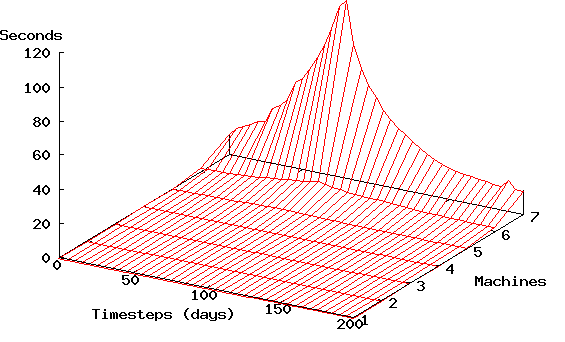
(b)

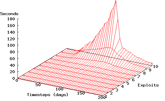
(c)

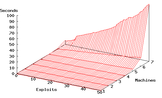
(d)

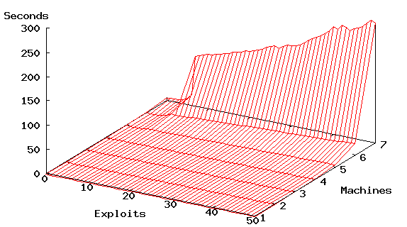
Figure 8: POMDP solver runtime ($z$ axis) when scaling: (a) time delay vs. the number of machines, (b) time delay vs. the number of exploits, (c) machines vs. exploits with time delay 10, and (d) machines vs. exploits with time delay 80.

Solving Penetration Testing with POMDPs

We now describe our experiments. We first fill in some details on the setup, then discuss different scaling scenarios, before having a closer look at some example policies generated by the POMDP solver.

Experiments Setup

The experiments are run on a machine with an Intel Core2 Duo CPU at 2.2 GHz and 3 GB of RAM. We use the APPL (Approximate POMDP Planning) toolkit. This C++ implementation of the SARSOP algorithm is easy to compile and use, and has reasonable performance. The solver is run without time horizon limit, until a target precision $\epsilon=0.001$ is reached. Since we are solving a stochastic shortest path problem, a discount factor is not required, however we use $\gamma=0.95$ to improve performance. We will briefly discuss below the effect of changing $\epsilon$ and $\gamma$.

Our problem generator is implemented in Python. It has 3 parameters:

number of machines $M$ in the target network,

number of exploits $E$ in the pentesting tool, that are applicable in the target network,

time delay $T$ since the last pentest, measured in days. For simplicity we assume that, at time $T=0$, the information about the network is perfect, i.e., there is no uncertainty. As $T$ grows, uncertainty increases as described in the previous section, where the parameters of the underlying model, cf. Fig. 7, are estimated by hand. The network topology consists of $1$ outside machine and $M-1$ other machines in a fully connected network. The configuration details are scaled along with $E$, i.e., details are added as relevant for the exploits (note that irrelevant configuration details would not serve any purpose in this application). As indicated, the exploits are taken from a Core Security database which contains the supported systems for each exploit (specific OS and application versions that are vulnerable). The $E$ exploits are distributed evenly over the $M$ machines. We require that $E\geq M$ so that each machine gets at least one exploit (otherwise the machine could be removed from the encoding).

Combined Scaling

We discuss performance—solver runtime—as a function of $M$, $E$, and $T$. To make data presentation feasible, at any one time we scale only 2 of the parameters.

Consider first Figure 8 (a), which scales $M$ and $T$. $E$ is fixed to the minimum value, i.e., each machine has a fixed OS version and one target application. In this setting, there are $3^{M}$ states. For $M=8$, the generated POMDP file has $6562$ states and occupies $71$ MB on disk; the APPL solver runs out of memory when attempting to parse it. Thus, in this and all experiments to follow, $M\leq 7$.

Naturally, runtime grows exponentially with $M$—after all, even the solver input does. As for $T$, interestingly this exhibits a very pronounced easy-hard-easy pattern. Investigating the reasons for this, we found that it is due to a low-high-low pattern of the “amount of uncertainty” as a function of $T$. Intuitively, as $T$ increases, the probability distribution in the initial belief state first becomes “broader” because more application updates are possible. Then, after a certain point, the probability mass accumulates more and more “at the end”, i.e., at the latest application versions, and the uncertainty decreases again. Formally, this can be captured in terms of the entropy of $b_{0}$, which exhibits a low-high-low pattern reflecting that of Figure 8 (a).

In Figure 8 (b), scaling the number $E$ of exploits as well as $T$, the number of machines is fixed to 2 (the localhost of the pentester, and one target machine. We observe the same easy-hard-easy pattern over $T$. As with $M$, runtime grows exponentially with $E$ (and must do so since the solver input does). However, with small or large $T$, the exponential behavior does not kick in until the maximum number of exploits, 10, that we consider here. This is important for practice since small values of $T$ (up to $T=50$) are rather realistic in regular pentesting. In the next sub-section, we will examine this in more detail to see how far we can scale $E$, in the 2-machines case, with small $T$.

Figure 8 (c) and (d) show the combined scaling over machines and exploits, for a favorable value of $T$ ($T=10$, (c)) and an unfavorable one ($T=80$, (d)). Here the behavior is rather regular. By all appearances, it grows exponentially in both parameters. An interesting observation is that, in (c), the growth in $M$ kicks in earlier, and rather more steeply, than in (d). Note that, in (d), the curve over $E$ flattens around $T=10$. We discuss this behavior in the next sub-section.

To give an impression on the effect of the discount factor on solver performance, with $M=2,E=11,T=40$, solver runtime goes from 17.77 s (with $\gamma=0.95$) to 279.65 s (with $\gamma=0.99$). APPL explicitly checks that $\gamma<1$, so $\gamma=1$ could not be tried. With our choice $\gamma=0.95$ we still get good policies (cf. further below).

The 2-Machines Case

As hinted, the 2-machines case is relevant because it may serve as the “atomic building block” in an industrial-scale solution, cf. also the discussion in the outlook below. The question then is whether or not we can scale the number of exploits into a realistic region. We have seen above already that this is not possible for unfavorable values of $T$. However, are these values to be expected in practice? As far as Core Security’s “Core Insight Enterprise” tool goes, the answer is “no”. In security aware environments, pentesting should be performed at regular intervals of at most 1 month. Consequently, Figure 9 shows data for $T\leq 50$.

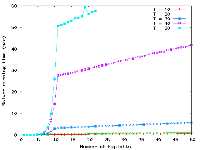
Figure 9: POMDP solver runtime when scaling the number of exploits, for different realistically small settings of the time delay, in the 2-machines case.

For the larger values of $T$, the data shows a very steep incline between $E=5$ and $E=10$, followed by what appears to be linear growth. This behavior is caused by an unwanted bias in our current generator. Ignoring this phenomenon, what matters to us here is that, for the most realistic values of $T$ ($T=10,20$), scaling is very good indeed, showing no sign of hitting a barrier even at $E=50$. Of course, this result must be qualified against the realism of the current generator. It remains an open question whether similar scaling will be achieved for more realistic simulations of network development.

POMDPs make Better Hackers

As an illustration of the policies found by the POMDP solver, consider a simple example wherein the pentester has 4 exploits: an SSH exploit (on OpenBSD, port 22), a wu-ftpd exploit (on Linux, port 21), an IIS exploit (on Windows, port 80), and an Apache exploit (on Linux, port 80). The probability of the target machine being Windows is higher than the probability of the other OSes.

Previous automated pentesting methods, e.g. Lucangeli et al. (?), proceed by first performing a port scan on common ports, then executing OS detection module(s), and finally launching exploits for potentially vulnerable services.

With our POMDP model, the policy obtained is to first test whether port 80 is open, because the expected reward is greater for the two exploits which target port 80, than for each of the exploits for port 21 or 22. If port 80 is open, the next action is to launch the IIS exploit for port 80, skipping the OS detection because Windows is more probable than Linux, and the additional information that OS Detect can provide doesn’t justify its cost (additional running time). If the exploit is successful, terminate. Otherwise, continue with the Apache exploit (not probing port 80 since that was already done), and if that fails then probe port 21, etc.

In summary, the policy orders exploits by promise, and executes port probe and OS detection actions on demand where they are cost-effective. This improves on Sarraute et al. (?), whose technique is capable only of ordering exploits by promise. What’s more, practical cases typically involve exploits whose outcome delivers information about the success probability of other exploits, due to common reasons for failure—exploitation prevention techniques. Then the best ordering of exploits depends on previous exploits’ outcome. POMDP policies handle this naturally, however it is well beyond the capabilities of Sarraute et al.’s approach. We omit the details for space reasons.

Discussion

POMDPs can model pentesting more naturally and accurately than previously proposed planning-based models (?; ?). While, in general, scaling is limited, we have seen that it appears reasonable in the 2-machines case where we are considering only how to get from one machine to another. An idea to use POMDP reasoning in practice is thus to perform it for all connected pairs of machines in the network, and thereafter use these solutions as the input for a high-level planning procedure. That procedure would consider the pairwise solutions to be atomic, i.e., no backtracking over these decisions would be made. Indeed, this is one of the abstractions made—successfully, as far as runtime performance is concerned—by Sarraute et al. (?). Our immediate future work will be to explore whether a POMDP-based solution of this type is useful, the question being how large the overhead for planning all pairs is, and how much of the solution quality gets retained at the global level.

A line of basic research highlighted by our work is the exploitation of special structures in POMDPs. First, in our model, all actions are deterministic. Second, some of the uncertain parts of the state (e.g. the operating systems) are static, for the purpose of pentesting, in the sense that none of the actions affect them. Third, unless one models possible detrimental side-effects of exploits (cf. directly below), pentesting is “monotonic”: accessibility, and thus the set of actions applicable, can only grow. Fourth, any optimal policy will apply each action at most once. Finally, some aspects of the state—in particular, which computers are controlled and reachable—are directly visible and could be separately modeled as being such. To our knowledge, this last property alone has been exploited in POMDP solvers (e.g., (?)), and the only other property mentioned in the literature appears to be the first one (e.g., (?)).

While accurate, our current model is of course not “the final word” on modeling pentesting with POMDPs. As already mentioned, we currently do not explicitly model the detrimental side-effects exploits may have, i.e., the cases where they are detected (spawning a reaction of the network defense) or where they crash a machine/application. Another important aspect that could be modeled in the POMDP framework is that machines are not independent. Knowing the configuration of some computers in the network provides information about the configuration of other computers in the same network. This can be modeled in terms of the probability distribution given in the initial belief. An interesting question for future research then is how to generate these dependencies—and thus the initial belief—in a realistic way. Answering this question could go hand in hand with more realistically simulating the effect of the “time delay” in pentesting. Both could potentially be adressed by learning appropriate graphical models (?), based on up-to-date real-world statistics.

To close the paper, it must be admitted that, in general, “pentesting $\neq$ POMDP solving”, by contrast to our paper title (hence the question mark). Computer security is always evolving, so that the probability of meeting certain computer configurations changes with time. An ideal attacker should continuously learn the probability distributions describing the network and computer configurations it can encounter. This kind of learning can be done outside the POMDP model, but there may be better solutions doing it more natively. Furthermore, if the administrator of a target network reacts to an attack, running specific counter-attacks, then the problem turns into an adversarial game.

References

- [Araya-López et al. 2010] Araya-López, M.; Thomas, V.; Buffet, O.; and Charpillet, F. 2010. A closer look at MOMDPs. In Proc. of ICTAI-10.
- [Arce and McGraw 2004] Arce, I., and McGraw, G. 2004. Why attacking systems is a good idea. IEEE Computer Society - Security & Privacy Magazine 2(4).
- [Bellman 1954] Bellman, R. 1954. The theory of dynamic programming. Bull. Amer. Math. Soc. 60:503–516.
- [Bilar 2003] Bilar, D. 2003. Quantitative Risk Analysis of Computer Networks. Ph.D. Dissertation, Dartmouth College.
- [Boddy et al. 2005] Boddy, M. S.; Gohde, J.; Haigh, T.; and Harp, S. A. 2005. Course of action generation for cyber security using classical planning. In Proc. of ICAPS’05.
- [Bonet 2009] Bonet, B. 2009. Deterministic POMDPs revisited. In Proc. of UAI’09.
- [Cassandra 1998] Cassandra, A. R. 1998. Exact and Approximate Algorithms for Partially Observable Markov Decision Processes. Ph.D. Dissertation, Brown University, Dept of Computer Science.
- [Dawkins and Hale 2003] Dawkins, J., and Hale, J. 2003. A systematic approach to multi-stage network attack analysis. In Proc. of DISCEX III.
- [Koller and Friedman 2009] Koller, D., and Friedman, N. 2009. Probabilistic Graphical Models: Principles and Techniques. MIT Press.
- [Kurniawati et al. 2008] Kurniawati, H.; Hsu, D.; and Lee, W. 2008. SARSOP: Efficient point-based POMDP planning by approximating optimally reachable belief spaces. In Robotics: Science and Systems IV.
- [Lucangeli et al. 2010] Lucangeli, J.; Sarraute, C.; and Richarte, G. 2010. Attack planning in the real world. In Workshop on Intelligent Security (SecArt 2010).
- [Lyon 1998] Lyon, G. F. 1998. Remote OS detection via TCP/IP stack fingerprinting. Phrack Magazine 8(54).
- [Monahan 1982] Monahan, G. 1982. A survey of partially observable Markov decision processes. Management Science 28:1–16.
- [Sarraute et al. 2011] Sarraute, C.; Richarte, G.; and Lucangeli, J. 2011. An algorithm to find optimal attack paths in nondeterministic scenarios. In ACM Workshop on Artificial Intelligence and Security (AISec’11).