The equilibrium allele frequency distribution for a population with reproductive skew

Abstract

We study the population genetics of two neutral alleles under reversible mutation in the $\Lambda$ processes, a population model that features a skewed offspring distribution. We describe the shape of the equilibrium allele frequency distribution as a function of the model parameters. We show that the mutation rates can be uniquely identified from the equilibrium distribution, but that the form of the offspring distribution itself cannot be uniquely identified. We also introduce an infinite-sites version of the $\Lambda$ process, and we use it to study how reproductive skew influences standing genetic diversity in a population. We derive asymptotic formulae for the expected number of segregating sizes as a function of sample size. We find that the Wright-Fisher model minimizes the equilibrium genetic diversity, for a given mutation rate and variance effective population size, compared to all other $\Lambda$ processes.

Introduction

Many questions in population genetics concern the role of demographic stochasticity in populations, and its interaction with mutation and selection in determining the fates of allelic types. The foundational work of Fisher, Wright, Haldane, Kimura [Fisher (1958, Wright (1931, Haldane (1932, Kimura (1994] and others has been instrumental in shaping our intuition about the powerful role that genetic drift plays in evolution, and especially its role in maintaining diversity. This classical theory, and the view of genetic drift as a strong force, emanates from the Wright-Fisher model of replication in a population, and its large-population limit, the Kimura diffusion [Kimura (1955]. The diffusion approximation has been particularly well-studied, not only because it is mathematically tractable, but also because it is robust to variation in many of the underlying model details. Many discrete population-genetic models, including a large number of Karlin-Taylor and Cannings processes [Karlin and McGregor (1964, Cannings (1974, Ewens (2004], share the same diffusion limit as the Wright-Fisher model, and they therefore exhibit qualitatively similar behavior.

Nevertheless, Kimura’s classical diffusion is not appropriate in every circumstance. Its central assumption is the absence of skew in the reproduction process — that is, the assumption that no single individual can contribute a sizable proportion to the composition of the population in a single generation. Several recent studies have suggested that this assumption may be violated in several species, especially in marine taxa but also including many types of plants [Beckenbach (1994, Hedgecock (1994], whose mode of reproduction involves a heavy-tailed offspring distribution.

While the number of empirical studies on heavy-tailed offspring distributions is limited, there is a rich mathematical theory to describe the dynamics of populations with heavy reproductive skew. Beginning with Cannings’ 1974 paper on neutral exchangeable reproduction processes, this literature has led to generalized notions of genetic drift, which subsume the traditional Wright-Fisherian concept of drift. The resulting forward-time continuum limits of such processes generalize the Kimura diffusion. One tractable class of models are the so-called $\Lambda$-Fleming-Viot processes, parameterized by a drift measure $\Lambda$. The corresponding backward-time, or coalescent theory, for such processes leads to the $\Lambda$-coalescents, first defined by Pittman and others [Pitman (1999, Sagitov (1999]. Two conspicuous features stand out in this more general theory: $\Lambda$ processes may have discontinuous sample paths, which feature “jumps” in the frequency of an allele, in contrast to the continuous sample paths of Kimura’s diffusion. Likewise, the coalescents of such processes typically exhibit multiple and even simultaneous mergers, instead of the strictly binary mergers of the classical Kingman coalescent.

Although mathematical aspects of such population processes (such as their construction, existence, uniqueness etc.) have already been described, the specific population-genetic consequences of reproductive skew have only recently begun to be worked out. In many cases, the classical picture of population genetics must be considerably enlarged to accommodate new phenomena — see for example [Möhle (2006] on generalizations of the Ewens’ sampling formula, [Eldon and Wakeley (2006b] on linkage disequilibrium in processes with skewed offspring distributions, [Birkner and Blath (2008, Birkner et al. (2011] on inference and sampling in the $\Lambda$ coalescent, and [Der et al. (2012] on the fixation probability of an adaptive allele in the $\Lambda$ process.

The purpose of this paper is to study the stationary allele frequency distribution for populations with reproductive skew, under neutrality. When there are a finite number of allelic types subject to mutation, allele frequencies evolve to a unique stationary distribution, and our principle aim will be to understand how this distribution depends on the form of reproductive skew, $\Lambda$, and how it may depart from the Wright-Fisherian picture.

Whereas a closed-form expression exists for the stationary allele frequency distribution in the (continuum) Wright-Fisher model, very few explicit expressions can be obtained in the general case of an arbitrary $\Lambda$ drift measure. Instead, we study the stationary distribution indirectly, first by deriving a recurrence relation satisfied by the moments in the two-allele scenario. This relation provides significant information about how the model parameters $(\theta,\Lambda)$ influence the stationary distribution. In particular, we demonstrate that the mutation parameters $\theta$ are identifiable from the stationary distribution, whereas the form of drift, $\Lambda$, is not in general identifiable.

We also study how reproductive skew alters the standing genetic diversity in a population at equilibrium. Some numerical experiments of ?), as well as some asymptotic results of ?) for the Beta-coalescent, have suggested that the Wright-Fisher model tends to minimize standing diversity, compared to other offspring distributions. To analyze this behavior, we develop a $\Lambda$-version of Kimura’s infinite-sites model, and we study the mean number of segregating sites, $\mathbb{E}S_{n}$, in a sample of size $n$. This measure of genetic diversity is robust in the sense that it is immune to many assumptions of the model and it coincides with the mean number of segregating sites in other infinite-sites models, including Watterson’s fully linked infinite-sites model. We demonstrate that the Wright-Fisher model minimizes diversity amongst all $\Lambda$-processes of the same variance-effective population size. In other words, reproductive skew always tends to amplify standing genetic diversity, compared to the classical population-genetic model. We also derive a recursion formula for the mean number of segregating sites, and we use this to obtain asymptotic formulae for the number of segregating sites in large samples.

The remainder of the paper is structured as follows. We start by reviewing discrete population models under reproductive skew. We then describe the forward-time continuum limits of such processes, which can be identified as $\Lambda$-Fleming-Viot processes. We develop a recursion equation for the moments of the stationary distribution in the two-allele case, and we use this to determine the identifiability of model parameters. To further examine equilibrium diversity we then introduce a two-allele, infinite-sites model with free recombination, and we study the frequency spectrum of samples from this process. This leads to a recursion formula for the mean number of segregating sites, and theorems concerning the minimization and maximization of diversity among all $\Lambda$ measures. We conclude by providing a simple intuition for our results, and by placing them in the context of the large literature on reproductive skew.

Discrete population models with reproductive skew

The $\Lambda$-models are generalizations of the classical Wright-Fisher and Moran processes, which incorporate the possibility of large family sizes in the offspring distribution. The characteristics of these processes are most easily understood by studying their continuum limits, described below. Nonetheless, we shall first describe these models and review their properties in a discrete setting, along the lines of the treatment in ?).

We consider a population containing a fixed number $N$ of individuals, each of two types. At every time step, a single individual is chosen uniformly from the population and produces a random number $U$ offspring, drawn from a distribution of offspring numbers, $P_{U}$. The subsequent generation is then comprised of the $U$ offspring from the chosen individual supplemented by $N-U$ other individuals, randomly selected without replacement from the remainder of the population. Only a single individual contributes offspring in each reproduction event — the remaining individuals who neither contribute offspring nor die simply persist to the next time step.

When the offspring distribution $P_{U}$ is concentrated at two individuals, i.e. $\mathbb{P}(U=2)=1$, this model coincides with the Moran process. More generally, we consider any discrete offspring number distribution $P_{U}$ supported on the set $\{0,\ldots,N\}$.

To incorporate mutation, an additional stage is appended after reproduction wherein each individual may mutate to the opposing type, independently and identically with a probability that depends upon the individual’s type, $\mu_{1}/N,\mu_{2}/N$, with $\mu_{i}\geq 0$. This composite process is graphically depicted in Figure 1. We shall term this discrete process a “generalized” Eldon-Wakeley model.

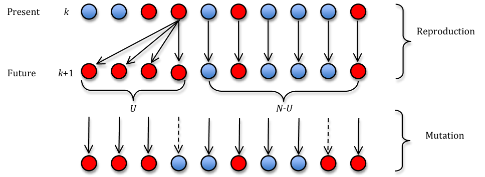
Figure 1: Schematic diagram of a discrete-time population model with reproductive skew.

The transition matrix.

We keep track of the number of individuals in generation $k$ of type 1, denoted by $X_{k}$. Since $X_{k}$ is a Markov chain on the states $\{0,\ldots,N\}$, it possesses an associated transition matrix $\mathbf{P}_{ij},0\leq i,j,\leq N$. The transition matrix $\mathbf{P}$ can be written as a product of two matrices,

$$\mathbf{P}=\mathbf{Q}\mathbf{M}$$ (1)

corresponding to the reproduction and mutation stages described above. The rows of the mutation matrix $\mathbf{M}$ are sums of independent binomial distributions, representing the mutational flux from each class. When all mutation rates are zero $\mathbf{M}=\mathbf{I}$, the identity matrix. The matrix $\mathbf{Q}$ describes the neutral genetic drift due to reproduction alone in the $\Lambda$-model; its form is more complex, with rows that are mixtures of hypergeometric distributions whose means depend on the offspring distribution $P_{U}$. An important quantity is the first row of $\mathbf{Q}$, called the “offspring distribution” of the process: $\mathbf{Q}_{1,j}$ for $j=0,1,\ldots N$. The variance of this distribution, called the “offspring variance” $\sigma^{2}_{N}$, determines the time-scaling of the continuum limit (see below).

Continuum approximations of population models with reproductive skew

Analysis of the Moran or Wright-Fisher model is facilitated by a continuum limit, which becomes accurate in the limit of large population size $N\rightarrow\infty$ [Kimura (1955, Ewens (2004]. As described in [Der et al. (2011], it is possible to derive a continuum limit for a significantly larger class of discrete population processes, including the $\Lambda$ models, without restrictions on the offspring distribution $P_{U}$. Similar work in the Cannings case has been developed by ?). While the limiting continuum processes are not, in general, diffusions with continuous sample paths, they are still characterized by an operator $G$, the infinitesimal generator of the continuum process, which reduces to the second-order differential equation of Kimura in the classical Wright-Fisher case.

Continuum approximations involve choosing how to scale time and space, as $N\rightarrow\infty$. Such scalings replace the number $i$ of individuals with the frequency $x=i/b_{N}$, and the generation number $k$ by the time $t=kc_{N}$, for some choices of sequences $\{b_{N}\},\{c_{N}\}$. The continuum limit is then the process

$$\tilde{X}_{t}=\lim_{N\rightarrow\infty}\frac{1}{b_{N}}X_{[t/c_{N}]}$$ (2)

In the classical Moran model we use the scalings $b_{N}=N$ and $c_{N}=N^{-2}$. In fact, it can be shown that the relationship between the space-scaling $b_{N}$ and time-scaling $c_{N}$ is fixed, in the sense that no other relationship leads to non-trivial limiting processes. We wish study allele frequencies, and hence impose the natural scaling $b_{N}=N$. The general theory [Möhle (2001, Der et al. (2011] then indicates that the time-scaling must be proportional to

$$c_{N}=\frac{\sigma^{2}_{N}}{N}$$ (3)

where $\sigma^{2}_{N}$ is the offspring variance of the $\Lambda$ process.

Once a time-scaling is fixed, then so is the appropriate scaling regime for the mutation rates, in order to produce a non-trivial balance of mutation and drift. This scaling must satisfy:

$$\mu_{i}=O(\sigma^{2}_{N})$$ (4)

In the classical Moran model $\sigma^{2}_{N}=1/N$, which produces the traditional scaling of mutation rate $\mu_{i}=O(N^{-1})$. In other models, such as the models of ?), where $\sigma^{2}_{N}=N^{-\gamma+1}$ and $\gamma<2$, mutation rates must scale faster to compensate for the increased rate of evolution from the drift process.

The limiting process for a generalized Eldon-Wakeley model.

By applying the techniques of [Der (2010, Möhle (2001], one may derive the continuum limit for the generalized Eldon-Wakeley process. These limits are characterized by an operator $G$, and an associated Kolmogorov backward equation, analogous to the diffusion equation of Kimura. We assume that we have a sequence of Eldon-Wakeley models, one for each population size $N$, and each with offspring distribution $P_{U}^{(N)}$. We assume the time-scaling and mutational constraints of (3) and (4) so that

$$\theta_{i}=\lim_{N\rightarrow\infty}\frac{2\mu_{i}}{\sigma_{N}^{2}}$$ (5)

defines the effective population-wide mutation rate. Under an appropriate condition on the sequence of offspring distributions $P_{U}^{(N)}$, there exists a limiting measure $\Lambda$ which may be derived from $\{P_{U}^{(N)}\}$ as:

$$\Lambda =\lim_{N\rightarrow\infty}\Lambda_{N}$$ (6)

$$\Lambda_{N}(i/N) =\left(\frac{i}{N}\right)^{2}P_{U}^{(N)}(i),\qquad i=0,\ldots,N$$ (7)

and which characterizes the continuum limit. Letting $\tilde{X}^{(N)}_{t}=\frac{1}{N}X_{[t/c_{N}]}$ denote the time and state re-scaled process, one can show then that $\tilde{X}^{(N)}_{t}$ converges to a limiting process $\tilde{X}_{t}$ that satisfies the backward equation:

$$\frac{\partial u(x,t)}{\partial t}=Gu(x,t),\qquad u(x,0)=f(x)$$ (8)

where

$$Gu(x)=\frac{1}{2}(-\theta_{1}x+\theta_{2}(1-x))\frac{\partial u}{\partial x}+\int_{0}^{1}\frac{xu(x+(1-x)\lambda)-u(x)+(1-x)u(x-\lambda x)}{\lambda^{2}}\,d\Lambda(\lambda)$$ (9)

and where $u(x,t)=\mathbb{E}[f(\tilde{X}_{t})|\tilde{X}_{0}=x]$.

The Markov process whose generator $G$ is given by (9) is called the forward-time, two-type $\Lambda$-Fleming-Viot process.

Intuitive remarks on the generator.

As with the matrix decomposition of (1), the generator of (9) splits into two terms: a portion $\frac{1}{2}(-\theta_{1}x+\theta_{2}(1-x))\frac{\partial}{\partial x}$ that describes mutation, independent of the reproduction measure $\Lambda$, and an integral portion that describes genetic drift. The term describing mutation coincides with the standard first-order advection term in Kimura’s diffusion equation. The integral term however, generally differs from the Kimura term, and it depends on the drift measure $\Lambda$.

Throughout the remainder of this paper we distinguish several important families of $\Lambda$-processes. We define the pure $\Lambda$ processes to be those models for which $\Lambda=\delta_{\lambda}$, the Dirac measure concentrated at a single point $\lambda$, with $0\leq\lambda\leq 1$. Since (9) expresses the generator as an integral decomposition over such Dirac measures, we can think a $\Lambda$-process as being a random mixture of these pure processes. Of particular interest are the extreme cases $\Lambda=\delta_{0}$, and $\Lambda=\delta_{1}$ — which correspond to the Wright-Fisher process and the so-called “star” processes, respectively. As we will show, these two processes constrain the range of dynamics in $\Lambda$ models. Another well-studied family in the coalescent literature are the Beta-processes, for which $\Lambda$ has a Beta distribution.

One can interpret $\Lambda$ as a “jump” measure controlling the frequency of large family sizes. If $\Lambda$ is concentrated near zero, then jump sizes are small. In this regime, the integrand $\frac{xu(x+(1-x)\lambda)-u(x)+(1-x)u(x-\lambda x)}{\lambda^{2}}$ behaves like the standard Kimura drift term $\frac{1}{2}x(1-x)u^{\prime\prime}(x)$. For the pure processes, where $\Lambda$ is concentrated at the point $\lambda$, allele frequencies remain constant for an exponential amount of time, until a bottleneck event in which a fraction $\lambda$ of the population is replaced by a single individual. Such events cause the allele frequency to increase instantaneously by the amount $(1-x)\lambda$, or decrease by $\lambda x$. In the most general case of an arbitrary measure $\Lambda$, these behaviors are mixed, and the jump events occur at exponential times with a random mean, and are associated with jumps of random size $\lambda$.

If $\Lambda$ places large mass near zero, the process becomes diffusion-like, with sample paths exhibiting frequent, small jumps. On the other hand, if $\Lambda$ is mostly concentrated away from zero then allele dynamics are of the “jump and hold” type, with fewer, but more sizable, jumps. Such behavior is most extreme in the star model, whose sample paths are constant until a single jump to absorption.

The Stationary Distribution of $\Lambda$-Processes

In the absence of mutation, $\mathbf{M}=\mathbf{I}$, allele frequencies must eventually fix at 0 or 1, and thus any discrete generalized Eldon-Wakeley model possesses a trivial stationary distribution whose concentration at the absorbing states $\{0,N\}$ depends on the initial condition. When mutation rates $\mu_{i}$ are strictly positive, however, each generalized Eldon-Wakeley process in a population size $N$ possesses a unique, non-trivial stationary distribution, $\pi_{N}$, to which the process converges, regardless of the initial condition.

In Figure 2, we plot the stationary distributions for a few $\Lambda$-processes, in the case of symmetric mutation $\theta_{1}=\theta_{2}$. Generally, these distributions have the same qualitative dependence on the mutation rate as the classical Wright-Fisher stationary distribution: they continuously progress from Dirac singularities at the boundaries to distributions concentrated more in the center of the interval, as the mutation rate increases. It is interesting to observe, however, that the non-Wright-Fisherian processes tend to have more mass at intermediate allele frequencies, and less relative mass near the boundaries, than the Wright-Fisherian model. We shall study this phenomenon more precisely, below.

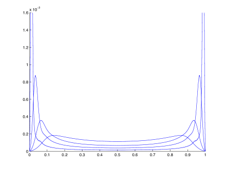
(a) Beta process ($\alpha=0.7,\beta=1$).

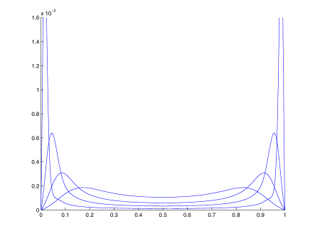
(b) Beta process ($\alpha=1.3,\beta=1$).

(c) Wright-Fisher (dashed), Beta (solid) processes,             $\alpha=0.7,\beta=1$.

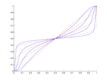
(d) Wright-Fisher (dashed), Beta (solid) processes,             $\alpha=1.3,\beta=1$.

Figure 2: Stationary Distributions for the Wright-Fisher and Beta processes. Top panels: stationary densities. Bottom panels, stationary cumulative distribution functions. Mutation values are $\theta=0.1,0.3,0.6,1.2$. Population size $N=8000$.

The continuum limit $\tilde{X}$ of a sequence of Eldon-Wakeley processes also possesses a unique stationary distribution, $\pi$. In the Appendix, we demonstrate that

$$\pi_{N}\rightarrow\pi,\quad\text{as }N\rightarrow\infty$$ (10)

In other words, the sequence of discrete equilibrium measures converges to the continuum equilibrium distribution. As a result, we can use the continuum equilibrium as a good approximation in large populations.

Moments of the Stationary Distribution.

In the case of two alleles, the stationary allele frequency distribution describes the likelihood of finding the mutant allele at any given frequency, at some time long in the future. We will study the moments of the stationary distributions for $\Lambda$ processes using a version of the Fokker-Planck equation, analogous to the equation used by Kimura to study the stationary distribution of the Wright-Fisher process. In general, a stationary distribution $\pi$ of a Markov process with generator $G$ is the solution to its so-called adjoint Fokker-Planck equation, so that

$$\int_{0}^{1}Gu(x)\,d\pi=0,$$ (11)

for every smooth function $u$ on $[0,1]$. We take $G$ as the generator for the $\Lambda$ process with mutation, given by (9). Although it is difficult to solve for $\pi$ in general, this equation can nonetheless be used to obtain detailed information about the stationary distribution.

To begin, we develop formulae for the moments of the stationary distribution, which will allow us to characterize aspects of standing genetic diversity. Let $m_{k}$ denote the $k$-th moment of $\pi$, $m_{k}=\int_{0}^{1}x^{k}\,d\pi(x)$. Setting $u(x)=x$ into (11) yields an equation for the mean value of the equilibrium, so that

$$m_{1}=\frac{\theta_{2}}{\theta_{1}+\theta_{2}}$$ (12)

Next, setting $u(x)=x^{2}$ into (11) yields a relation between $m_{2}$ and $m_{1}$,

$$m_{2}=\frac{(1+\theta_{2})\theta_{2}}{(\theta_{1}+\theta_{2})(1+\theta_{1}+\theta_{2})}$$ (13)

This recursive process can be continued, because the generator $G$ of (9) maps polynomials of degree $k$ to polynomials of degree $k$. Thus, we can derive a system of equations that define the moments of $\pi$. In the appendix, we show that this recursion has the form:

$$m_{k}=\frac{\left(\frac{k}{2}\theta_{2}+a_{k-1,k}\right)m_{k-1}+\sum_{j=1}^{k-2}a_{jk}m_{j}}{\frac{k}{2}(\theta_{1}+\theta_{2})+a_{kk}}$$ (14)

where the coefficients $\{a_{jk}\}$, $1\leq j\leq k$, $k=1,2,\ldots$, are functions of $\Lambda$, and are given by

$$a_{kk} =\int_{0}^{1}\frac{1-(1-\lambda)^{k}-k\lambda(1-\lambda)^{k-1}}{\lambda^{2}}\,d\Lambda(\lambda)$$ (15)

$$a_{j,k} =\binom{k}{j-1}\int_{0}^{1}\lambda^{k-j-1}(1-\lambda)^{j-1}\,d\Lambda(\lambda),\qquad j=1,\ldots,k-1$$ (16)

Initializing this system by (12), and observing that $a_{kk}>0$, we see that (14) uniquely determines the moments of $\pi$, and indeed this equation can be used to solve for any specific moment of the stationary distribution. While it does not appear that the moments $m_{k}$ can be solved explicitly to produce simple, closed-form expressions as functions of the $\Lambda$ measure, it is clear that the coefficients $a_{jk}$ are all linear combinations of moments of $\Lambda$. Moreover, each moment $m_{k}$ is always a ratio of polynomials in $\theta_{1}$ and $\theta_{2}$.

Identifiability of parameters from equilibrium.

One of the most important questions about the stationary allele frequency distribution is what population-genetic parameters can be identified from it — that is, which parameters of the population can be uniquely determined from data sampled in equilibrium? In the case of $\Lambda$ processes, the parameters we might wish to infer are the mutation rates, $\theta_{1}$ and $\theta_{2}$, as well as the (high-dimensional) drift measure, $\Lambda$, which describes the offspring distribution.

The first two moments of the stationary distribution are given by (12) and (13), and they are independent of the drift measure, $\Lambda$. Thus, the first- and second-order moments of the stationary distribution for all $\Lambda$-processes, and any function of these moments, such as the second-order heterozygosity $\int_{0}^{1}x(1-x)d\pi(x)$, must coincide with those of the classic Wright-Fisher model. In the case of symmetric mutation $\theta_{1}=\theta_{2}=\theta$, the third moment is also, remarkably, constant across the $\Lambda$-processes, and has the value

$$m_{3}=\frac{2+\theta}{4+8\theta}.$$ (17)

The constancy of the first two moments with respect to $\Lambda$, and the fact that the mapping from the first two moments to the two mutation parameters $(m_{1},m_{2})\mapsto(\theta_{1},\theta_{2})$ given by (12) and (13) is one-to-one, allows us to conclude that, regardless of the underlying reproductive process, the mutation rates $(\theta_{1},\theta_{2})$ are always identifiable from the equilibrium distribution. This is a tremendously productive result — because it means that we can always infer mutation rates from sampled data, even when the offspring distribution of a species is unknown to us.

Conversely, we may ask whether we can identify the form of reproductive process without knowledge of mutation rates — that is, is $\Lambda$ uniquely identifiable from the stationary distribution alone? It turns out that the answer is negative, as we demonstrate with the following simple example.

Consider the star process $\Lambda=\delta_{1}$ with mutation parameters $\theta_{1}=\theta_{2}=\theta$. The generator for this process is

$$Gu(x)=\frac{1}{2}\theta(1-2x)u^{\prime}(x)+(1-x)u(0)-u(x)+xu(1)$$ (18)

The associated stationary distribution $\pi_{1}$ is easily derived (see Appendix), and it has a density $d\pi_{1}/dx$ given by

$$\frac{d\pi_{1}}{dx}=\frac{1}{\theta}|1-2x|^{\frac{1-\theta}{\theta}}$$ (19)

For comparison, the Kimura diffusion has a Dirichlet-type stationary distribution $\pi_{0}$:

$$\frac{d\pi_{0}}{dx}=\frac{\Gamma(2\theta)}{(\Gamma(\theta))^{2}}x^{\theta-1}(1-x)^{\theta-1}$$ (20)

Note that both distributions (19) and (20) coincide when $\theta=1$, despite the enormous difference between the drift measures of these processes. Hence, the map from a given $\Lambda$ process to its stationary distribution is not one-to-one, and consequently the drift measure $\Lambda$ cannot generally be identified from the stationary distribution. This is a pessimistic result, because it implies that that the offspring distribution and form of genetic drift cannot in general be inferred from data collected in equilibrium, even when the mutation rate is known.

An infinite-sites model for the $\Lambda$-processes

In order to understand how reproductive skew influences standing genetic diversity, we now develop an infinite-sites version of the $\Lambda$ process and study its equilibrium behavior. This model generalizes the infinite-sites approach of [RoyChoudhury and Wakeley (2010, Desai and Plotkin (2008], for the Wright-Fisher model. We will study the sampled site frequency spectrum of our model, under two-way mutation. Our analysis will allow us to quantify our previous observation that the Wright-Fisher model minimizes the amount of standing genetic diversity, amongst all $\Lambda$ processes. The site frequency spectrum that we will describe in this section, for independent sites, differs from the Watterson-type spectrum for fully linked sites; but our approach nonetheless yields information in that case as well.

We consider an evolving population of large size $N$, following the reproduction dynamics of a neutral forward-time $\Lambda$-process, for a fixed $\Lambda$ measure. We keep track of $L$ sites along the genome, each with two possible allelic types under symmetric two-way mutation at rates $\theta=\theta_{1}=\theta_{2}$. The allele dynamics at each site are described by a two-type $\Lambda$-process; and the site processes are assumed independent of one another (that is, we assume free recombination).

Let $\pi_{\theta}$ denote the two-allele stationary distribution for the $\Lambda$ model, given by (11), where the subscript denotes the explicit dependence on the mutation rate. We imagine sampling $n$ individuals from the population at equilibrium, assuming $n\ll N$. We let $Y_{i}$, $1\leq i\leq L$ represent the (random) number of sampled individuals at site $i$ with a particular allelic type, so that their joint distribution has the form

$$P(Y_{1}=y_{1},\ldots,Y_{L}=y_{L})=\prod_{i=1}^{L}\int_{0}^{1}\binom{n}{y_{i}}x^{y_{i}}(1-x)^{n-y_{i}}\,d\pi_{\theta}(x)$$ (21)

The sampled site frequency spectrum [Sawyer and Hartl (1992, Bustamante et al. (2001] is defined as the vector $(Z_{0},\ldots,Z_{n})$

$$Z_{k}=\sum_{i=1}^{L}1_{Y_{i}=k},\quad k=0,\ldots,n$$ (22)

The variables $Z_{k}$ record the number of sites with precisely $k$ (out of $n$) sampled individuals of a given allelic type. In this sense, the sampled site frequency spectrum represents a discretized version of the stationary distribution $\pi_{\theta}$. The variables $(Z_{0},\ldots,Z_{n})$ are distributed multinomially on the simplex $\sum_{k=0}^{n}Z_{k}=L$. The sites $Z_{1},\ldots,Z_{n-1}$ are called the segregating sites, representing locations where there is diversity observed in the the sample. Conversely, the sum $Z_{0}+Z_{n}$ represents the number of monomorphic sites in the sample.

The infinite-site limit and its Poisson representation.

To study the sampled site frequency spectrum we take the limit of an infinite number of sites, $L\rightarrow\infty$, and we apply a Poisson approximation. We define the genome-wide mutation rate as $\Theta_{L}=L\cdot\theta$, and we assume that this mutation rate approaches a constant in the limit of many sites: $\Theta_{L}\rightarrow\Theta<\infty$. In the Appendix, we show that the segregating site variables $(Z_{1},\ldots,Z_{n-1})$ then converge, as $L\rightarrow\infty$, to a sequence of independent Poisson random variables with means $(c_{1}\Theta,\ldots,c_{n-1}\Theta)$, given by

$$c_{j}(n)=\lim_{\theta\rightarrow 0}\frac{1}{\theta}\int_{0}^{1}\binom{n}{j}x^{j}(1-x)^{n-j}\,d\pi_{\theta}(x),\qquad j=1,\ldots,n-1$$ (23)

The numbers $c_{j}$ may be interpreted as an infinite-sites sample frequency spectrum. From (23), it is apparent that the means $c_{j}$ depend on the heterozygotic moments of $\pi$, and thus, also on the moments of $\Lambda$. This representation is thus a generalization of a result of ?) for the two-allele Wright-Fisher independent-sites model, where $\Lambda=\delta_{0}$, and where the spectrum $c_{j}$ has the form $c_{j}=\frac{1}{2}\frac{n}{j(n-j)}$ for $j=1,\ldots,n-1$.

For the Wright-Fisher model, ?) has shown that the number of segregating sites in the sample of size $n$, $S_{n}=\sum_{i=1}^{n-1}Z_{i}$, is a sufficient statistic for $\Theta$, under the independent-sites assumption. This is an important result because the number of segregating sites vastly compresses the information in the frequency spectrum, yet nonetheless contains no loss of information for the purposes of inferring the mutation rate. The Poisson representation of the sample frequency spectrum we have derived shows that $S_{n}$ remains Poisson distributed even in the general $\Lambda$ infinite-sites case — under the assumption of site independence. Thus, the sufficiency of $S_{n}$ for $\Theta$ remains true, and consequently $S_{n}$ possesses desirable qualities for robust estimation of $\theta$.

Diversity amplification and the number of segregating sites.

The number of segregating sites in a sample is a classic and powerful method to quantify genetic diversity in a population. Here we study how $S_{n}$ depends on the form of reproduction — that is, on the form of the drift measures $\Lambda$. In particular, we will show that the Wright-Fisher model minimizes the expected number of segregating sites in a sample, compared to all other $\Lambda$ processes. Thus, large family sizes in the offspring distribution will tend to amplify the amount of diversity in a population.

Under the infinite-sites Poisson approximation, the number of segregating sites $S_{n}$ in a sample of size $n$ is Poisson-distributed, and its expected value is

$$\mathbb{E}S_{n}=\mathbb{E}\sum_{j=1}^{n-1}Z_{j}=\Theta\sum_{j=1}^{n-1}c_{j}(n)$$ (24)

where $c_{j}(n)$ are the coefficients in (23). The binomial theorem applied to (23) then shows that:

$$\mathbb{E}S_{n}=\lim_{\theta\downarrow 0}\frac{1}{\theta}\int_{0}^{1}[1-x^{n}-(1-x)^{n}]\,d\pi_{\theta}(x)$$ (25)

and so we may interpret the expected number of segregating sites as a type of higher-order heterozygosity statistic of the stationary distribution. According to (23), $c_{j}(n)$ is a linear combination of moments of $\pi$, of order at most $n$. It follows that the average number of segregating sites may be evaluated by the recursion (14) and it can be expressed as rational functions of moments of $\Lambda$. The first several such expressions are listed below:

$$\mathbb{E}S_{2} =\Theta$$ (26)

$$\mathbb{E}S_{3} =\frac{3}{2}\cdot\Theta$$ (27)

$$\mathbb{E}S_{4} =\frac{\int_{0}^{1}(5\lambda^{2}-14\lambda+11)\,d\Lambda(\lambda)}{\int_{0}^{1}(6-8\lambda+3\lambda^{2})\,d\Lambda(\lambda)}\cdot\Theta$$ (28)

$$\mathbb{E}S_{5} =\frac{5}{2}\frac{\int_{0}^{1}(5-6\lambda+2\lambda^{2})\,d\Lambda(\lambda)}{\int_{0}^{1}(6-8\lambda+3\lambda^{2})\,d\Lambda(\lambda)}\cdot\Theta$$ (29)

$$\mathbb{E}S_{6} =\frac{1}{2}\frac{\int_{0}^{1}(2608\lambda^{2}-1558\lambda+411-2428\lambda^{3}+1312\lambda^{4}-388\lambda^{5}+49\lambda^{6})\,d\Lambda(\lambda)}{\int_{0}^{1}(6-8\lambda+3\lambda^{2})(15-40\lambda+45\lambda^{2}-24\lambda^{3}+5\lambda^{4})\,d\Lambda(\lambda)}\cdot\Theta$$ (30)

$$\vdots$$

These expressions for the expected number of segregating sites become extremely complex for larger sample sizes $n$. Nevertheless, we can use asymptotic methods to study how diversity is expected to behave in large sample sizes. We will address two primary questions. First, how does does the expected number of segregating sites, $\mathbb{E}S_{n}$, grow as a function of the sample size, for a given drift-measure $\Lambda$? And second, which reproduction processes $\Lambda$ maximize and minimize $\mathbb{E}S_{n}$, for fixed $\Theta$?

In the appendix, we use the moment recursion (14) to derive the following recursion for the sequence $\{\mathbb{E}S_{n}\},n=2,3,\ldots$

$$\mathbb{E}{S}_{n}=\frac{n\Theta}{2a_{nn}}+\sum_{j=1}^{n-1}\frac{a_{jn}}{a_{nn}}\mathbb{E}S_{j}$$ (31)

with the initial value $\mathbb{E}S_{1}=0$, and where $\{a_{jn}\}$ are given by (15) and (16). We can use this relation to obtain detailed information about $\mathbb{E}S_{n}$ both as a function of the sample size $n$, and as a function of the underlying $\Lambda$ measure.

Consider first the pure $\Lambda$ processes $\Lambda=\delta_{\lambda}$, in which a single individual may replace a given fixed fraction $0<\lambda\leq 1$ of the population. Then we can prove from (31) that (see Appendix):

$$\mathbb{E}S_{n}=\frac{\lambda\Theta}{2}n+O(\log n),\qquad n\rightarrow\infty$$ (32)

Two features are of interest in this asymptotic expression. First, the average number of segregating sites grows linearly with sample size in a pure $\Lambda$ process, as opposed to logarithmically as in the Wright-Fisher case. Second, the rate of linear growth depends on the jump fraction, $\lambda$, so that asymptotically, diversity is maximized for large replacement fractions $\lambda$, and correspondingly minimized when this fraction is small.

Equation (32) can be generalized to a larger class of $\Lambda$ measures. If $\Lambda$ is any probability measure whose support excludes a neighborhood of zero, then we have the asymptotic formula:

$$\mathbb{E}S_{n}=C(\Lambda)\Theta\cdot n+O(\log n),\qquad n\rightarrow\infty$$ (33)

where $C(\Lambda)=(2\int_{0}^{1}\lambda^{-1}\,d\Lambda)^{-1}$. This equation shows that linear growth of the expected number of segregating sites is characteristic of any $\Lambda$ process whose drift measure is bounded away from zero — that is, any $\Lambda$ process that does not contain a component of the Wright-Fisher process. This result allows us to determine which reproduction processes $\Lambda$ maximize and minimize the average number of segregating sites $\mathbb{E}S_{n}$, for a given value of $\Theta$. In the appendix, we prove the following optimization principle: for each sample size $n$, the diversity maximizing and minimizing processes within the class of all $\Lambda$ processes must in fact be pure $\Lambda$ processes, i.e. where $\Lambda$ is concentrated at a single point. It follows then from (32) that, asymptotically, the Wright-Fisher model ($\lambda=0$) minimizes, and the star-model ($\lambda=1$) maximizes, respectively, the mean number of segregating sites amongst all $\Lambda$-processes.

Although these results apply in the limit of large sample sizes, we conjecture that the Wright-Fisher and star models are also the extremal diversity processes for any sample size, $n$. From the optimization principle stated above, it suffices to check this statement within the restricted class of pure $\Lambda$ processes. In Figure 3, we show $\mathbb{E}S_{n}/\Theta$ as a function of the jump-size parameter $\lambda$ for the pure models, for a few values of $n$. These results confirm that the Wright-Fisher model minimizes $\mathbb{E}S_{n}$, whereas the star model maximizes $\mathbb{E}S_{n}$, over all $\Lambda$-models. We have conducted numerical studies which support this proposition more generally, even for very small sample sizes. In this sense, the Wright-Fisher model and star models are extremal processes, and, for a given effective variance population size, respectively minimize and maximize the expected genetic diversity in any sample.

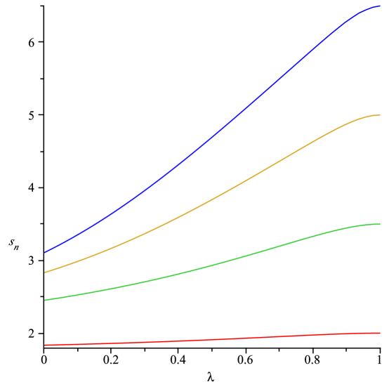
Figure 3: Diversity $s_{n}=\mathbb{E}S_{n}/\Theta$ versus jump-size $\lambda$ in the pure $\Lambda$ processes, for $n=4,7,10,13$ (bottom to top). These functions attain their extrema at the endpoints $0$ and $1$, implying that the Wright-Fisher and star processes minimize and maximize diversity for these sample sizes.

Discussion

We have studied the stationary distribution of a very general class of population models, under mutation. We have focused on understanding the interaction between the form of the offspring distribution and resulting form of genetic drift it engenders, as well as the shape of the stationary distribution. We have demonstrated that the mutation rate can always be uniquely identified from the stationary distribution, even when the drift measure is unknown (as it always will be, in practice). However, the form of the drift measure $\Lambda$ cannot always be uniquely identified from equilibrium properties of the process — and so may require dynamic data to determine its specific form.

The stationary allele frequency distribution of the Wright-Fisher process is extremal, in a sense, within the class of $\Lambda$-processes. Specifically, the Wright-Fisher model exhibits greater probability mass near very high and low allele frequencies. This observation was formalized by analyzing a $\Lambda$ infinite-sites model, in which we found that the mean number of segregating sites in a sample is indeed minimized by the Wright-Fisher process.

Our results can be placed in the context of a nascent literature that views the Wright-Fisher process as an extremal model within the large space of possible population processes. Aside from the diversity-minimization property we have demonstrated here, it has previously been observed, for instance, that among $\Lambda$-processes, the Wright-Fisher model minimizes the fixation probability of an adaptive allele [Der et al. (2012], minimizes the time to absorption for new mutants [Der et al. (2011], and, among generalized coalescents, possesses the fastest rate of “coming down from infinity” [Berestycki et al. (2010]. The basic intuition behind all these results revolves around the type of sample paths possessed by different processes. A typical sample path in the Kimura diffusion undergoes a high frequency of small jumps (in fact, is continuous), and thus new mutants persist for only $O(\log N)$ generations before being eliminated by genetic drift. By contrast, in a general $\Lambda$ model with the same variance effective population size, large jumps in the sample path may occur, but with lower frequency, thereby lengthening the absorption time — for example, up to order $N$ generations in the pure $\Lambda$ processes. Since the mean number of segregating sites in the entire population is the product of the genomic mutation rate and the expected absorption time for a new mutant, standing genetic diversity must increase when reproductive skew is present.

Although we have presented results only within the class of $\Lambda$-processes, many of our formulae — for example (14) – can be generalized to the set of all Cannings models. We expect the diversity-minimization property of the Wright-Fisher model will hold even within this larger family.

The infinite-sites model of the $\Lambda$-process we have developed here differs from the Watterson infinite-sites model typically encountered in coalescent theory, in two respects. First, we have assumed free recombination and hence independent sites, whereas in Watterson’s model sites are tightly linked. Second, we assume two-way mutation between alternative alleles at each site, whereas Watterson’s model features one-way mutation at each site away from the existing type. Nonetheless, some of the results derived for our site-independent, infinite-sites model extend to the Watterson, linked infinite-sites $\Lambda$ processes as well.

In general, the (random) number of segregating sites $S_{n}$ in a sample is a function of the dependency structure among sites. For example, in the simple Wright-Fisherian case, independence of sites gives rise to a Poisson distribution for $S_{n}$, compared to a sum of geometric random variables in the case of no recombination [Ewens (2004]. However, as ?) has already remarked, the mean value of $S_{n}$ is generally robust to the recombination structure of an infinite-sites model. If $Y_{1},\ldots,Y_{L}$ denote the allelic distributions at $L$ sites, then (22) shows that the expected number of segregating sites is a function only of the marginal distributions of $Y_{i}$, instead of their joint distribution. Thus the expected number of segregating sites in a sample is unaffected by linkage. Likewise, the distinction between one-way and two-way mutation (and folded and unfolded spectra) does not alter the mean number of segregating sites other than by a possible overall scaling.

Because $S_{n}$ is such a common measure of genetic diversity, our results have some connections to the literature on $\Lambda$-coalescents. Recently, ?) showed that, for those $\Lambda$ measures whose coalescent comes down from infinity, the (random) number of segregating sites $S_{n}$ in a sample of size $n$ for the Watterson model has the asymptotic law:

$$\frac{S_{n}}{\int_{0}^{n}q\psi^{-1}(q)dq}\rightarrow\Theta$$ (34)

where $\psi$ is the Laplace exponent of the $\Lambda$ measure, defined as:

$$\psi(q)=\int_{0}^{1}\frac{\exp(-q\lambda)-1+q\lambda}{\lambda^{2}}d\Lambda$$ (35)

The authors conjectured that (34) holds more generally, even when $\Lambda$ does not come down from infinity. In this respect, our asymptotic result (33) for $\mathbb{E}S_{n}$ — derived for $\Lambda$ measures bounded away from zero (and thus always fail to come down from infinity) is evidence in favor of their more general conjecture, in the case not covered by the hypotheses of their theorem. For under such assumptions, the Laplace exponent has the expression

$$\psi(q)\sim q\int_{0}^{1}\lambda^{-1}\,d\Lambda$$ (36)

which implies from (34) that

$$\int_{0}^{n}q\psi^{-1}(q)\,dq\sim n\cdot\left(\int_{0}^{1}\lambda^{-1}d\Lambda\right)^{-1}$$ (37)

which is proportional with our formula (33) for $\mathbb{E}S_{n}$. Finally, returning to the case of independent sites, developed in this paper, it is also true that the distributional convergence of (34) holds, a fact which follows from the Poisson representation for $S_{n}$.

In our analysis of the expected number of segregating sites, we have concentrated on the two extreme cases— the Wright-Fisher case, for which $\mathbb{E}S_{n}$ is known to grow logarithmically in the sample size $n$, and the case of pure $\Lambda$ processes (and more generally those $\Lambda$ processes whose drift measure support excludes zero), for which we have demonstrated linear growth of $\mathbb{E}S_{n}$. Nevertheless, the recurrence relation (31) can be used to analyze intermediary cases as well, for example the Beta processes, in which the density of $\Lambda$ behaves like a power-law in the vicinity of zero. For such reproduction measures, growth in diversity with sample size will lie somewhere between the logarithmic and the linear cases.

Appendix

The Stationary Distribution of Processes with Reproductive Skew.

Let $X^{(N)}$ be a sequence of discrete generalized Eldon-Wakeley processes, one for each population size $N$, converging to a continuum $\Lambda$ process $\tilde{X}$, under the state and time re-normalization of (3), (4). If we suppose that each discrete process operates under strictly positive mutation rates $\mu_{i}^{(N)}$, then it is easily verified that the associated forward-time transition matrices $\mathbf{P}^{(N)}$ possess strictly positive entries, and thus, from the Perron-Frobenius theorem, there exists a unique stationary distribution $\pi_{N}$ for each process $X^{(N)}$. A standard argument, using the fact that the sequence $\pi_{N}$ is tight, shows that there is a subsequence $\pi_{N_{k}}$ converging to a probability measure $\pi$ which is a stationary distribution for $\tilde{X}$ (see ?), for example). This argument indeed demonstrates that any weak limit point of $\pi_{N}$ is a stationary distribution $\tilde{X}$; below, through the moment recursion, this distribution is uniquely characterized, and hence every weakly convergent subsequence of $\pi_{N}$ converges to $\pi$, thus $\pi_{N}\rightarrow\pi$.

Derivation of a Recursion for the Moments of the Stationary Distribution.

Let $\pi$ be the stationary distribution for the two-type $\Lambda$ process, which satisfies (11). In this section we obtain a recursion formula for the moments of $\pi$.

Define the operator $Lu(x)=xu(x+(1-x)\lambda)-u(x)+(1-x)u(x-\lambda x)$. Setting $u(x)=x^{k}$, $k\geq 0$ we have

$$Lx^{k} =((1-\lambda)^{k}-1)x^{k}-(1-\lambda)^{k}x^{k+1}+x(x+(1-x)\lambda)^{k}$$

$$=((1-\lambda)^{k}-1)x^{k}-(1-\lambda)^{k}x^{k+1}+x^{k+1}(1-\lambda)^{k}+kx^{k}(1-\lambda)^{k-1}\lambda+\sum_{j=0}^{k-2}\binom{k}{j}x^{j+1}(1-\lambda)^{j}\lambda^{k-j}$$

$$=((1-\lambda)^{k}-1+k\lambda(1-\lambda)^{k-1})x^{k}+\sum_{j=1}^{k-1}\binom{k}{j-1}x^{j}(1-\lambda)^{j-1}\lambda^{k-j+1}$$ (38)

Separating the $\Lambda$ generator (9) into the mutation and pure-drift portions, we define the latter to be the operator

$$G_{D}u(x)=\int_{0}^{1}\frac{1}{\lambda^{2}}Lu(x)d\Lambda(\lambda).$$ (39)

If we write

$$G_{D}x^{k}=\sum_{j=1}^{k}b_{jk}x^{j}$$ (40)

Then substituting (38) into (39), and then comparing the coefficients to (40) , we have

$$b_{kk} =\int_{0}^{1}\frac{(1-\lambda)^{k}+k\lambda(1-\lambda)^{k-1}-1}{\lambda^{2}}\,d\Lambda(\lambda)$$ (41)

$$b_{jk} =\binom{k}{j-1}\int_{0}^{1}\lambda^{k-j-1}(1-\lambda)^{j-1}\,d\Lambda(\lambda),\qquad j<k$$ (42)

Let $\pi$ be any stationary distribution of the process. Then according to (11),

$$\int_{0}^{1}\left[\frac{1}{2}(-\theta_{1}x+\theta_{2}(1-x))kx^{k-1}+G_{D}x^{k}\right]d\pi(x)=0$$ (43)

Using the expansion for $G_{D}x^{k}$ above, we derive:

$$\left(b_{kk}-\frac{k}{2}(\theta_{1}+\theta_{2})\right)m_{k}+\left(\frac{k}{2}\theta_{2}+b_{k-1,k}\right)m_{k-1}+\sum_{j=1}^{k-2}b_{jk}m_{j}=0$$ (44)

where $m_{j}$ is the $j$-th moment of the $\pi$. This is equivalent to formulae (14), (15) and (16), where $b_{kk}=-a_{kk}$, and $b_{jk}=a_{jk}$ for $j<k$.

Derivation of the star-process stationary distribution.

Consider the probability measure $\mu$ on $[0,1]$, with density

$$\frac{d\mu}{dx}=\frac{1}{\theta}|1-2x|^{\frac{1-\theta}{\theta}}$$ (45)

The generator for the star-process undergoing symmetric mutation is $Gu=\frac{1}{2}\theta(1-2x)u^{\prime}(x)+(1-x)u(0)-u(x)+xu(1)$, and the space of twice continuously differentiable functions $C^{2}[0,1]$ is a core for $G$. Noting that the density $d\mu/dx$ satisfies the equation $-d/dx(\frac{\theta}{2}(1-2x)d\mu/dx)-d\mu/dx=0$ and integrating by parts, it is readily verified that $\int_{0}^{1}Gu\,d\mu=0$ for every $u\in C^{2}$. Thus $\mu$ is a stationary distribution for the process, and is further unique as established by the moment recursion (44).

Poisson representation of the infinite-sites model.

In this section we show that the segregating site variables $(Z_{1},\ldots,Z_{n-1})$ in the independent sites $\Lambda$ model converge to a sequence of Poisson random variables with means $(c_{1}\Theta,\ldots,c_{n-1}\Theta)$, given by (23). We make use of the structure of the moments of the stationary distribution as found in (14). First we require a preliminary lemma.

Lemma 1.

Let $\pi_{\theta}$ be the stationary distribution of a $\Lambda$ process undergoing symmetric mutation $\theta$. Then there exist constants $c_{j}\geq 0$, for $1\leq j\leq n-1$,

$$p_{j}(\theta)=\int_{0}^{1}\binom{n}{j}x^{j}(1-x)^{n-j}\,d\pi_{\theta}(x)=c_{j}\theta+o(\theta),\quad\theta\downarrow 0$$ (46)

Proof.

The lemma is equivalent to saying $p_{j}(0)=0$ and $p_{j}$ has a derivative at $\theta=0$. First observe from (14) that under $\theta_{1}=\theta_{2}$, all the moments $m_{k}(\theta)$ of the stationary distribution are differentiable in $\theta$ for all $\theta\geq 0$, and hence $p_{j}(\theta)$ is differentiable everywhere. Also

$$|p_{j}(\theta)|\leq\binom{n}{j}\int_{0}^{1}x(1-x)\,d\pi_{\theta}(x)=\binom{n}{j}\frac{2\theta}{1+2\theta}$$ (47)

hence $p_{j}(\theta)\rightarrow 0$ as $\theta\downarrow 0$.   

Now to establish the Poisson representation, it is enough to apply the well-known Poisson approximation to the multinomial distribution. We use:

Theorem 1.

[McDonald (1980]. If $(Z_{0},\ldots,Z_{n})$ is multinomial with parameters $(L,p_{0},\ldots,p_{n})$, and $(V_{1},\ldots,V_{n-1})$ are independent Poissons with means $Lp_{j}$, then

$$\|(Z_{1},\ldots,Z_{n-1})-(V_{1},\ldots,V_{n-1})\|\leq 2L\left(\sum_{j=1}^{n-1}p_{j}\right)^{2}$$ (48)

where $\|\cdot\|$ is the total variation norm of measures.

The Poisson representation is now obvious, since $p_{j}(\theta)=O(\theta)=O(1/L)$ by Lemma 1 and therefore the right-hand side of (48) goes to zero as $L\rightarrow\infty$. Since $(V_{1},\ldots,V_{n-1})$ are converging to a sequence of independent Poisson distributions with finite means $c_{j}\Theta$, where $c_{j}$ are as in Lemma 1, so must $(Z_{1},\ldots,Z_{n-1})$.

The average number of segregating sites.

In this section, we study the number of segregating sites $S_{n}$ in the infinite-sites $\Lambda$ model, deriving the recursion (31) for the average diversity measure $s_{n}=\mathbb{E}S_{n}/\theta$, and use it to obtain asymptotic expressions for diversity.

Let $\pi_{\theta}$ be the stationary distribution of the $\Lambda$ process under two way symmetric mutation $\theta$. Define $H_{n}(\theta)$ as the heterozygosity measure

$$H_{n}(\theta)=\sum_{j=1}^{n-1}\int_{0}^{1}\binom{n}{j}x^{j}(1-x)^{n-j}\,d\pi_{\theta}(x)$$ (49)

Applying the binomial theorem,

$$H_{n}(\theta)=\int_{0}^{1}(1-x^{n}-(1-x)^{n})\,d\pi_{\theta}(x)=\int_{0}^{1}(1-2x^{n})\,d\pi_{\theta}(x)$$ (50)

where the second equality follows from symmetry of the stationary distribution. Now, define the diversity measure $s_{n}\equiv\mathbb{E}S_{n}/\Theta$. We have from (25):

$$s_{n}=\lim_{\theta\downarrow 0}\frac{1}{\theta}H_{n}(\theta)$$ (51)

Under symmetric mutation $\theta=\theta_{1}=\theta_{2}$, the recursion formulae for moments (14) reads

$$m_{n}(\theta)=\frac{n\theta+\sum_{j=1}^{n-1}a_{jn}m_{j}(\theta)}{n\theta+a_{nn}}$$ (52)

From symmetry of the stationary distribution and differentiability of $m_{n}$, there are numbers $\{v_{n}\}$ such that $m_{n}(\theta)=1/2+v_{n}\theta+O(\theta^{2})$. Inserting this into the right-hand side of (52), and expanding in a Taylor series, we obtain, by comparing the first-order coefficients, a recursion for $v_{n}$:

$$v_{n}=\frac{-n/4+\sum_{j=1}^{n-1}a_{jn}v_{j}}{a_{nn}}$$ (53)

The equations (50) and (51) imply that $s_{n}=-2v_{n}$. Thus the corresponding recursion for $\{s_{n}\}$ is

$$s_{n}=\frac{n/2+\sum_{j=1}^{n-1}a_{jn}s_{j}}{a_{nn}}$$ (54)

where we initialize $s_{1}=0$. Observe that by the binomial theorem, one has the relation

$$a_{nn}=\sum_{j=1}^{n-1}a_{jn}$$ (55)

Thus the numbers $a_{jn}/a_{nn}$ define a probability measure on the set $j\in\{1,\ldots,n-1\}$. By studying this measure and the recurrence relation defining $s_{n}$, we may derive the asymptotics for $s_{n}$.

Now suppose that the underlying $\Lambda$ process is associated with a $\Lambda$ measure with support bounded away from zero. Then from (15), $a_{nn}=\int_{0}^{1}\lambda^{-2}d\Lambda+O(\gamma^{n})$, for some $0<\gamma<1$. Therefore, $a_{nn}^{-1}=\left(\lambda^{-2}d\Lambda\right)^{-1}+O(\gamma^{n})$. Using this estimate in the recursion (51), and defining $A=\left(\int_{0}^{1}\lambda^{-2}d\Lambda\right)^{-1}$,

$$s_{n}=An/2+A\sum_{j=1}^{n-1}a_{jn}s_{j}+O(\gamma^{n})$$ (56)

Now, we shall prove

Theorem 2.

$$s_{n}=Cn+O(\log n),\qquad n\rightarrow\infty$$ (57)

where

$$C=\frac{A}{2-2A\int_{0}^{1}\lambda^{-2}(1-\lambda)\,d\Lambda}$$ (58)

Proof.

Let $s_{n}=Cn+g_{n}$. We find, using the explicit expressions (16),

$$Cn+g_{n}=An/2+A\sum_{j=1}^{n-1}\int_{0}^{1}\lambda^{-2}\binom{n}{j-1}\lambda^{n-(j-1)}(1-\lambda)^{j-1}\,d\Lambda\cdot(Cj+g_{j})+O(\gamma^{n})$$ (59)

The right-hand side of the above is

$$An/2+A\sum_{j=1}^{n+1}\int_{0}^{1}Cj\lambda^{-2}\binom{n}{j-1}\lambda^{n-(j-1)}(1-\lambda)^{j-1}d\Lambda+A\sum_{j=1}^{n-1}\int_{0}^{1}g_{j}\lambda^{-2}\binom{n}{j-1}\lambda^{n-(j-1)}(1-\lambda)^{j-1}d\Lambda+O(\gamma^{n})$$ (60)

where we have subtracted two binomial terms and exponentially bounded them. Using the formula for the mean of a binomial random variable with parameters $(n,1-\lambda)$ in the first series, this is equivalent to

$$An/2+An\int_{0}^{1}C(1-\lambda)\lambda^{-2}d\Lambda+A\sum_{j=1}^{n-1}\int_{0}^{1}g_{j}\lambda^{-2}\binom{n}{j-1}\lambda^{n-(j-1)}(1-\lambda)^{j-1}d\Lambda+O(1)$$ (61)

Inserting this expression into (59), dividing by $n$, and using the definition of $C$, we find that $g_{n}$ satisfies the relation

$$g_{n}=A\sum_{j=1}^{n-1}\int_{0}^{1}g_{j}\lambda^{-2}\binom{n}{j-1}\lambda^{n-(j-1)}(1-\lambda)^{j-1}d\Lambda+O(1/n)$$ (62)

Completing the series with two binomial terms once more,

$$g_{n}=A\int_{0}^{1}\lambda^{-2}(\mathbb{E}_{\lambda,n}g)\,d\Lambda+O(1/n)$$ (63)

where the expectation occurs with respect to a binomial random variable with parameters $(n,1-\lambda)$. We may further interpret the integral term as an expectation of $g$ under a mixture of binomials with mixing weights $1/\lambda^{2}$.

We can now prove that that $g_{n}=O(\log n)$. To be explicit in (63), let $B$ be a constant such that

$$\left|g_{n}-A\int_{0}^{1}\lambda^{-2}(\mathbb{E}_{\lambda,n}g)\,d\Lambda\right|\leq B/n$$ (64)

for all $n$. We shall show, by induction, that $g_{n}\leq B\log n$, for large $n$. By enlargening $B$, the base case $g_{0}$ is satisfied. Assume that the statement it is true up to $n$. Then using Jensen’s inequality on the mixture in (63),

$$g_{n+1}\leq B\log\left(A\int_{0}^{1}\lambda^{-2}(1-\lambda)n\,d\Lambda\right)+B/n$$ (65)

If $\epsilon>0$ is a number smaller than $\inf\text{supp }\Lambda$, then we can, keeping in mind the definition of $A$, further bound this expression by:

$$g_{n+1} \leq B\log((1-\epsilon)n)+B/n$$ (66)

$$=B\log((1-\epsilon)n)+B\log(n+1)-B\log(n)+O(1/n^{2})$$ (67)

$$\leq B\log(n+1)$$ (68)

Thus Theorem 2 is proved.   

The constant $C$ in Theorem 2 is algebraically equivalent to $C(\Lambda)$ in (33).

An Optimization Principle for the average number of segregating sites.

In this section we prove the following theorem:

Theorem 3.

For every sample size $n$, and for fixed mutation rate $\Theta$, the minimum and maximum values of $\mathbb{E}S_{n}$ over the class of $\Lambda$ processes is achieved within the class of pure Eldon-Wakeley processes; that is, where $\Lambda=\delta_{\lambda}$, for $0\leq\lambda\leq 1$.

Proof.

It is evident from the recursion for $\mathbb{E}S_{n}$ in (54) that the average number of segregating sites must have the form:

$$\mathbb{E}S_{n}/\Theta=\frac{\int_{0}^{1}f_{n}(\lambda)\,d\Lambda}{\int_{0}^{1}g_{n}(\lambda)\,d\Lambda}$$ (69)

for some functions (in fact, polynomials) $f_{n},g_{n}$. Because $\mathbb{E}S_{n}$ is positive for every pure Eldon-Wakeley process (where $\Lambda=\delta_{\lambda}$), we can without loss of generality assume that $f_{n},g_{n}\geq 0$. For such functions, we have the lemma:

Lemma 2.

For positive functions $f,g$ defined on $[0,1]$, we have the inequalities:

$$\min_{\lambda}\frac{f(\lambda)}{g(\lambda)}\leq\frac{\int_{0}^{1}f(\lambda)\,d\Lambda}{\int_{0}^{1}g(\lambda)\,d\Lambda}\leq\max_{\lambda}\frac{f(\lambda)}{g(\lambda)}$$ (70)

Proof.

We prove the lower bound; the upper bound is established in the same way. Say $\Lambda$ is a two-point measure: $\Lambda=p_{1}\delta_{\lambda_{1}}+p_{2}\delta_{\lambda_{2}}$. Then elementary manipulations show

$$\frac{p_{1}f(\lambda_{1})+p_{2}f(\lambda_{2})}{p_{1}g(\lambda_{1})+p_{2}g(\lambda_{2})}\geq\text{min }\{f(\lambda_{1})/g(\lambda_{1}),f(\lambda_{2})/g(\lambda_{2})\}$$ (71)

By induction one easily generalize to measures concentrated at any finite number of points. Finally, the full case is obtained by taking weak limits of measures concentrated at a finite number of points.   

Returning to the proof of the main theorem, one sees that Lemma 2 immediately implies the result, since $f_{n}(\lambda)/g_{n}(\lambda)$ is precisely $\mathbb{E}S_{n}/\Theta$ for the case $\Lambda=\delta_{\lambda}$.   

The optimization principle can be refined. Let $\Lambda$ be any probability measure whose support excludes a neighborhood of zero, and suppose that $\lambda_{\text{min}}$ and $\lambda_{\text{max}}$ are the smallest and largest values, respectively, on which $\Lambda$ is supported, i.e. $\lambda_{\text{min}}=\inf\text{supp }\Lambda$, and $\lambda_{\text{max}}=\sup\text{supp }\Lambda$. Then

$$\frac{\lambda_{\text{min}}}{2}\leq C(\Lambda)\leq\frac{\lambda_{\text{max}}}{2}$$ (72)

In conjunction with (33), this shows that the asymptotic growth rate in $\mathbb{E}S_{n}$ for a $\Lambda$ -process whose drift measure is supported on the interval $[\lambda_{min},\lambda_{max}]$ can be lower and upper-bounded by the rates of growth in $\mathbb{E}S_{n}$ of two pure processes, with parameters $\lambda_{min}$ and $\lambda_{max}$, respectively. In other words, the effect of mixing any two pure $\Lambda$ processes always results in a process whose equilibrium diversity is intermediate relative to the diversities of the pure models.

LITERATURE CITED

- Beckenbach (1994 Beckenbach, A., 1994 Mitochondrial haplotype frequencies in oysters: neutral alternatives to selection models. Genetics and evolution of aquatic organisms: 122–134.
- Berestycki et al. (2007 Berestycki, J., J. Berestycki, and J. Schweinsberg, 2007 Beta-Coalescents and Continuous Stable Random Trees. The Annals of Probability 35: 1835–1887.
- Berestycki et al. (2010 Berestycki, J., N. Berestycki, and V. Limic, 2010 The -coalescent speed of coming down from infinity. Annals of Probability 38: 207–233.
- Berestycki et al. (2012 Berestycki, J., N. Berestycki, and V. Limic, 2012 Asymptotic sampling formulae for -coalescents. arXiv 1201.6512.
- Birkner and Blath (2008 Birkner, M. and J. Blath, 2008 Computing likelihoods for coalescents with many collisions in the infinitely many sites model. Journal of Mathematical Biology 57: 435–465.
- Birkner et al. (2011 Birkner, M., J. Blath, and M. Steinrucken, 2011 Importance sampling for Lambda-coalescents in the infinitely many sites model. Theoretical Population Biology 79: 155–173.
- Bustamante et al. (2001 Bustamante, C. D., J. Wakeley, S. Sawyer, and D. L. Hartl, 2001 Directional Selection and the Site-Frequency Spectrum. Genetics 159: 1779–1788.
- Cannings (1974 Cannings, C., 1974 The Latent Roots of Certain Markov Chains Arising in Genetics: A New Approach, I. Haploid Models. Adv. Appl. Prob. 6(2): 260–290.
- Der (2010 Der, R., 2010 A Theory of Generalised Population Processes, Ph. D. Thesis. Philadelphia: ProQuest.
- Der et al. (2012 Der, R., C. Epstein, and J. Plotkin, 2012 Dynamics of neutral and selected alleles when the offspring distribution is skewed. Genetics 191: 1331–1344.
- Der et al. (2011 Der, R., C. L. Epstein, and J. B. P. Plotkin, 2011 Generalized Population Processes and the Nature of Genetic Drift. Theor. Pop. Biol. 80: 80–99.
- Desai and Plotkin (2008 Desai, M. M. and J. B. Plotkin, 2008 The polymorphism frequency spectrum of finitely many sites under selection. Genetics 180(4): 2175–2191.
- Eldon and Wakeley (2006a Eldon, B. and J. Wakeley, 2006a Coalescent Processes when the Distribution of Offspring Number Among Individuals is Highly Skewed. Genetics 172: 2621–2633.
- Eldon and Wakeley (2006b Eldon, B. and J. Wakeley, 2006b Linkage disequilibrium under skewed offspring distribution among individuals in a population. Genetics 178: 1517–1532.
- Ethier and Kurtz (1986 Ethier, S. N. and T. G. Kurtz, 1986 Markov processes: characterization and convergence. Hoboken: Wiley Interscience.
- Ewens (2004 Ewens, W. J., 2004 Mathematical population genetics (2nd ed.). New York: Springer.
- Fisher (1958 Fisher, R. A., 1958 The genetical theory of natural selection. New York: Dover Publications.
- Haldane (1932 Haldane, J., 1932 A Mathematical Theory of Natural and Artificial Selection, Part IX, Rapid Selection. Proc. Camb. Phil. Soc. 28: 244–248.
- Hedgecock (1994 Hedgecock, D., 1994 Does variance in reproductive success limit effective population size of marine organisms? Non-neutral evolution: 188–198.
- Karlin and McGregor (1964 Karlin, S. and J. McGregor, 1964 Direct product branching processes and related markov chains. Proc. Natl. Acad. Sci. U.S.A. 51: 598–602.
- Kimura (1955 Kimura, M., 1955 Solution of a process of random genetic drift with a continuous model. Proc. Natl. Acad. Sci. 41: 144–150.
- Kimura (1994 Kimura, M., 1994 Population Genetics, Molecular Evolution, and the Neutral Theory: Selected Papers. Chicago: The University of Chicago Press.
- McDonald (1980 McDonald, D., 1980 On the Poisson approximation to the multinomial distribution. Canadian Journal of Statistics 8: 115–118.
- Möhle (2001 Möhle, M., 2001 Forward and backward diffusion approximations for haploid exchangeable population models. Stoch. Proc. Appl. 95: 133–149.
- Möhle (2006 Möhle, M., 2006 On sampling distributions for coalescent processes with simultaneous multiple collisions. Bernoulli 1: 35–53.
- Pitman (1999 Pitman, J., 1999 Coalescents with Multiple Collisions. Annals of Probability 27: 1870–1902.
- RoyChoudhury and Wakeley (2010 RoyChoudhury, A. and J. Wakeley, 2010 Sufficiency of the number of segregating sites in the limit under finite-sites mutation. Theoretical Population Biology 78: 118–122.
- Sagitov (1999 Sagitov, S., 1999 The General Coalescent with Asynchronous Mergers of Ancestral Lines. Journal of Applied Probability 36: 1116–1125.
- Sawyer and Hartl (1992 Sawyer, S. A. and D. L. Hartl, 1992 Population genetics of polymorphism and divergence. Genetics 132: 1161–1176.
- Watterson (1975 Watterson, G. A., 1975 On the number of segregating sites in genetical models without recombination. Theoretical population biology 7: 256–276.
- Wright (1931 Wright, S., 1931 Evolution in Mendelian populations. Genetics 16: 97–159.