Galerkin Methods for Complementarity Problems and
Variational Inequalities  

Abstract

Complementarity problems and variational inequalities arise in a wide variety of areas, including machine learning, planning, game theory, and physical simulation. In all of these areas, to handle large-scale problem instances, we need fast approximate solution methods. One promising idea is Galerkin approximation, in which we search for the best answer within the span of a given set of basis functions. Bertsekas [1] proposed one possible Galerkin method for variational inequalities. However, this method can exhibit two problems in practice: its approximation error is worse than might be expected based on the ability of the basis to represent the desired solution, and each iteration requires a projection step that is not always easy to implement efficiently. So, in this paper, we present a new Galerkin method with improved behavior: our new error bounds depend directly on the distance from the true solution to the subspace spanned by our basis, and the only projections we require are onto the feasible region or onto the span of our basis.

1 Background

1.1 Definitions

We first define variational inequalities and complementarity problems [2]. We consider here only problems defined over convex feasible sets, although it is possible to define analogous problems over nonconvex sets.

A cone is a set $K$ such that, for any $\lambda\geq 0$ and $x\in K$, we have $\lambda x\in K$. The dual cone of $K$ is

$$K^{*}=\{y\mid\forall x\in K,\,x^{\top}y\geq 0\}$$

For any set $C$ and point $x\in C$, the normal cone to $C$ at $x$ is $N_{C}(x)=\{d\mid d^{\top}(y-x)\leq 0,\,\forall y\in C\}$.

Definition 1.1 (Variational inequality)

Given a nonempty closed convex set $C$ and an operator $F$, the variational inequality VI$(F,C)$ is to find $x$ s.t.:

$$x \in C$$

$$-F(x) \in N_{C}(x)$$

The VI is linear if $F(x)=Mx+q$.

In a complementarity problem, the feasible set $K$ is required to be a cone. Define $(x,y)$ to be $K$-complementary if $x\in K$, $y\in K^{*}$, and $x^{\top}y=0$. Then the complementarity problem asks us to find a $K$-complementary pair $(x,F(x))$:

Definition 1.2 (Complementarity problem)

Given a nonempty closed convex cone $K$ and an operator $F$, the complementarity problem CP$(F,K)$ is to find $x$ s.t.:

$$x \in K$$

$$F(x) \in K^{*}$$

$$x^{\top}F(x) =0$$

The CP is linear if $F(x)=Mx+q$.

A common choice is to take $K$ to be the nonnegative orthant; in this case complementarity means that, for all $i$, at least one of $x_{i}$ and $[F(x)]_{i}$ is zero.

1.2 Relationships

Variational inequalities and complementarity problems are strongly related. First, if the feasible set of a variational inequality is a cone $K$, then VI$(F,K)$ is equivalent to CP$(F,K)$; that is, both problems have the same set of solutions. Second, if the feasible set is the intersection of a cone $K$ with some equality constraints $Ax=b$, then we can eliminate the equality constraints using Lagrange multipliers: VI$(F,K\cap\{x\mid Ax=b\})$ is equivalent to VI$(\bar{F},\bar{K})$, where $\bar{K}=K\times\mathbb{R}^{m}$ and

$$\bar{F}(x,\lambda)=\left(\begin{array}[]{c}F(x)-A^{\top}\lambda\\ Ax-b\end{array}\right)$$

Since we can represent any convex set as the intersection of a cone with equality constraints, the above relationships mean that we can transform any VI to a CP and vice versa.

For computational purposes, it is often convenient to transform our problem so that the feasible set is a very simple cone. For example, for the polyhedron $\{x\mid Ax+b\geq 0\}$, we introduce a vector of nonnegative slack variables $s$ and write $Ax+b=s$, with $x$ free and $s\geq 0$. After eliminating the equality constraints with Lagrange multipliers, our feasible set is the cone $K=\{(s,x,\lambda)\mid s\geq 0\}$. This cone is separable: it is the product of one-dimensional cones. The advantage of this sort of transformation is that it is extremely efficient to work with separable cones: e.g., Euclidean projection onto $K$ just means thresholding each component of $s$ at $0$.

1.3 Complexity

If we assume that the feasible set $K$ is a separable cone, then the computational complexity of a variational inequality or complementarity problem depends on the operator $F$. Even if $F$ is restricted to be linear, it is possible to encode NP-hard problems. An important class that ensures polynomial-time solvability is the class of monotone operators:

Definition 1.3

An operator $F$ is monotone on the set $C$ if, for some $\beta\geq 0$,

$$(x-y)^{\top}(F(x)-F(y)) \geq\beta\|x-y\|^{2}\quad\forall x,y\in C$$

It is strongly monotone if the above holds with $\beta>0$.

A linear operator $F(x)=Mx+q$ is monotone iff $M$ is positive semidefinite, and strongly monotone iff $M$ is positive definite. (There is no requirement for $M$ to be symmetric.)

Among Lipschitz operators (which include all finite-dimensional linear operators), strong monotonicity implies a useful contraction property:

Lemma 1.1

If the operator $F$ is $\beta$-strongly monotone and $L$-Lipschitz on some set $C$, and if we take $\alpha=\beta/L^{2}$, then the operator $I-\alpha F$ is Lipschitz on $C$ with constant $\gamma=\sqrt{1-\beta^{2}/L^{2}}<1$.

Proof: For any $x,y\in C$,

$$\|(x-\alpha F(x))-(y-\alpha F(y))\|^{2}$$

$$=\|(x-y)-\alpha(F(x)-F(y))\|^{2}$$

$$=\|x-y\|^{2}-2\alpha(x-y)^{\top}(F(x)-F(y))$$

$$\qquad{}+\alpha^{2}\|F(x)-F(y)\|^{2}$$

$$\leq\|x-y\|^{2}-2\alpha\beta\|x-y\|^{2}+\alpha^{2}L^{2}\|x-y\|^{2}$$

$$=(1-2\alpha\beta+\alpha^{2}L^{2})\|x-y\|^{2}$$

Choosing $\alpha$ to minimize the RHS, we have $\alpha=\beta/L^{2}$; the square of the Lipschitz constant is then

$$1-2\alpha\beta+\alpha^{2}L^{2}=1-\beta^{2}/L^{2}<1$$

as claimed. $\Box$

This contraction property means that a very simple algorithm, the projection method, converges linearly to the solution of our variational inequality, as we will see in the next section.

2 Projection method

In a variational inequality, the condition that $-F(x)$ is in the normal cone to $C$ at $x$ is equivalent to

$$x =\Pi_{C}(x-\alpha F(x))$$ (1)

where $\alpha$ is any nonnegative step size and $\Pi_{C}$ represents Euclidean projection onto the set $C$. That is, if we take a step in the direction $-F(x)$ and project back onto $C$, we don’t move. More formally:

Lemma 2.1

If $x=\Pi_{C}(x+d)$ for some step $d$, then $d\in N_{C}(x)$.

(We omit the proof.)

The projection method simply treats (1) as an assignment: start from an arbitrary $x^{(0)}$, then for $t=1,2,\ldots$, set

$$x^{(t)} =T(x^{(t-1)})\equiv\Pi_{C}(x^{(t-1)}-\alpha F(x^{(t-1)}))$$ (2)

(We could also choose a separate step size $\alpha_{t}$ for each step $t$, but for simplicity we ignore this possibility.)

The projection method converges linearly for strongly-monotone $F$, since its update operator is a contraction:

Lemma 2.2

In the projection method, suppose the operator $(I-\alpha F)$ is $\gamma$-Lipschitz. Then the variational inequality (1) has a unique solution $x^{*}$. Furthermore, for any $\epsilon>0$, if we take $t\geq\ln(\epsilon)/\ln(\gamma)$ steps of the projection method, we will have $\|x^{(t)}-x^{*}\|\leq\epsilon\|x^{(0)}-x^{*}\|$.

Proof: The update operator $T=\Pi_{C}\circ(I-\alpha F)$ is $\gamma$-Lipschitz, since it is the composition of a projection operator (which is $1$-Lipschitz) with $(I-\alpha F)$. Existence and uniqueness of the solution follow from the contraction mapping theorem; for the error bound,

$$\|x^{(t)}-x^{*}\| =\|Tx^{(t-1)}-Tx^{*}\|$$

$$\leq\gamma\|x^{(t-1)}-x^{*}\|$$

$$\leq\gamma^{t}\|x^{(0)}-x^{*}\|$$

That is, the distance between $x^{(t)}$ and $x^{*}$ reduces by a factor $\gamma$ with each application of $T$. Substituting the assumed value for $t$ now yields the desired bound. $\Box$

3 Galerkin method—I

If the dimension of $x$ is very large, each iteration of the projection method may be too slow to be practical. The problem is exacerbated if $\gamma$ is close to 1. In this case, it makes sense to search for a Galerkin approximation, i.e., an approximate solution within the span of some basis matrix $\Phi$. The hope is that we can design an approximate projection method that will find such a solution much more cheaply than the raw projection method.

Bertsekas [1] proposed one such Galerkin approximation: assume that $\hat{C}\equiv\mathop{\text{\rm span}}(\Phi)\cap C$ is nonempty, and define the approximation as the fixed point of

$$x^{(t)} =\hat{T}(x^{(t-1)})\equiv\Pi_{\hat{C}}(x^{(t-1)}-\alpha F(x^{(t-1)}))$$ (3)

Compared to (2), we simply project onto $\hat{C}$ instead of $C$ at each iteration. Note that (3) also defines an algorithm for computing the Galerkin approximation, although not the only possible one.

If the dimension of $x$ is $n$, but the rank of $\Phi$ is $k<n$, we may be able to implement the iteration (3) cheaply: e.g., for a linear variational inequality, we can precompute $\Phi^{\top}M\Phi$ and $\Phi^{\top}q$, and work in $k$-dimensional space instead of $n$-dimensional space. The only caveat is projection onto $\hat{C}$; depending on the forms of $\Phi$ and $C$, this projection may or may not be possible to implement efficiently.

Essentially the same convergence rate analysis holds for the Bertsekas-Galerkin projection method as for the original projection method:

Lemma 3.1

Suppose $(I-\alpha F)$ is $\gamma$-Lipschitz and $\hat{C}$ is nonempty. Then the iteration (3) has a unique fixed point, say $\hat{x}$; and, we need at most $t\geq\ln(\epsilon)/\ln(\gamma)$ iterations to achieve error $\|x^{(t)}-\hat{x}\|\leq\epsilon\|x^{(0)}-\hat{x}\|$.

Proof: Identical to the proof of Lemma 2.2. $\Box$

In addition, we can prove a bound on the distance between the approximate solution $\hat{x}$ and the original solution $x^{*}$:

Lemma 3.2

For the Bertsekas-Galerkin method, the error between the approximate solution $\hat{x}$ and the true solution $x^{*}$ satisfies:

$$\|\hat{x}-x^{*}\| \leq\|\Pi_{\hat{C}}(x^{*})-x^{*}\|/(1-\gamma)$$ (4)

Proof: Note that $\hat{T}(x)=\Pi_{\hat{C}}(T(x))$, and $T(x^{*})=x^{*}$. So, $\hat{T}(x^{*})=\Pi_{\hat{C}}(T(x^{*}))=\Pi_{\hat{C}}(x^{*})$, and

$$\|\hat{T}(x^{*})-x^{*}\| =\|\Pi_{\hat{C}}(x^{*})-x^{*}\|$$

Applying $\hat{T}$ repeatedly to both $x^{*}$ and $\hat{T}(x^{*})$, and using the fact that $\hat{T}$ is $\gamma$-Lipschitz, we have

$$\|\hat{T}(\hat{T}(x^{*}))-\hat{T}(x^{*})\| \leq\gamma\|\Pi_{\hat{C}}(x^{*})-x^{*}\|$$

$$\|\hat{T}^{t}(x^{*})-\hat{T}^{t-1}(x^{*})\| \leq\gamma^{t-1}\|\Pi_{\hat{C}}(x^{*})-x^{*}\|$$

So, after $t$ iterations, we have

$$\|\hat{T}^{t}(x^{*})-x^{*}\| \leq\sum_{i=1}^{t}\|\hat{T}^{i}(x^{*})-\hat{T}^{i-1}(x^{*})\|$$

$$\leq\sum_{i=1}^{t}\gamma^{i-1}\|\Pi_{\hat{C}}(x^{*})-x^{*}\|$$

$$\leq\|\Pi_{\hat{C}}(x^{*})-x^{*}\|/(1-\gamma)$$

where the last line follows by summing a geometric series. Since this inequality holds for all $t>0$, it holds in the limit as $t\to\infty$, yielding (4). $\Box$

The bound (4) depends on $\|\Pi_{\hat{C}}(x^{*})-x^{*}\|$, a measure of our representation error—that is, how closely we can approximate $x^{*}$ in our low-dimensional representation.

Qualitatively, compared to the exact projection method, the Bertsekas-Galerkin method tightens the feasible region and relaxes the optimality condition: both the iterates $x^{(t)}$ and the approximate solution $\hat{x}$ will be exactly feasible. (In fact, they will be in $\hat{C}\subseteq C$.) But, at convergence, the step direction $-F(\hat{x})$ will not necessarily be in a normal cone of $C$, as it would in the exact solution. Instead, Lemma 2.1 means that the step direction will be in the normal cone to $\hat{C}$ at $\hat{x}$.

Another way to interpret this approximate optimality criterion is that, since $\hat{C}=C\cap\mathop{\text{\rm span}}(\Phi)$ is the interection of two sets, the normal cone to $\hat{C}$ is the sum of their two normal cones, $N_{C}(\hat{x})+\mathop{\text{\rm null}}(\Phi^{\top})$. In other words, for some residual vector $\epsilon\in\mathop{\text{\rm null}}(\Phi^{\top})$, we have that $-F(\hat{x})+\epsilon$ is in the normal cone to $C$ at $\hat{x}$.

4 Galerkin method—II

While the error bound (4) is nice to have, it is less than perfectly satisfying: the representation error measure $\|\Pi_{\hat{C}}(x^{*})-x^{*}\|$ may be quite large, even if $\mathop{\text{\rm span}}(\Phi)$ passes close to $x^{*}$. See Fig. 1 for an example. An extreme version of this problem is that $\mathop{\text{\rm span}}(\Phi)$ might not even intersect the feasible set $C$.

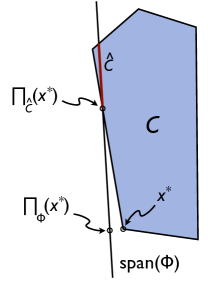
Figure 1: Illustration of error bound (4).

To remedy this problem, in this section we propose a simple new Galerkin method, and bound the new method’s convergence rate and error. Our new method’s bounds will depend on a different measure of representation error, based on projection onto $\mathop{\text{\rm span}}(\Phi)$ instead of $\hat{C}$. Since $\mathop{\text{\rm span}}(\Phi)\supseteq\hat{C}$, we expect this change to lead to an improvement in the bound: for any given vector $z$, the error $\|\Pi_{\Phi}(z)-z\|$ will be no larger, and sometimes much smaller, than the error $\|\Pi_{\hat{C}}(z)-z\|$.

To enable projection onto $\mathop{\text{\rm span}}(\Phi)$ instead of $\hat{C}$, we modify the algorithm as described below; in particular, we project the proposed update $z=x-\alpha F(x)$ instead of the proposed solution $x$. When $\alpha$ is small, we have $z\approx x$, so that $\|z-\Pi_{\Phi}(z)\|\lesssim\|x-\Pi_{\hat{C}}(x)\|$. For larger $\alpha$ it is possible that this inequality could be reversed; but in our (limited) experience, even for larger $\alpha$, the new method’s bounds are at least as tight as those of the Bertsekas-Galerkin method, and often much tighter.

In more detail, our approximation is based on the following re-arrangement of the projection method: pick $z^{(0)}$ or $x^{(0)}$ arbitrarily, and for all $t=1,2,\ldots$, repeat:

$$x^{(t-1)} =\Pi_{C}(z^{(t-1)})$$ (5)

$$z^{(t)} =x^{(t-1)}-\alpha F(x^{(t-1)})$$ (6)

It is easy to see that the sequence $x^{(t)}$ computed by this iteration is the same as the one computed by (2), so long as we start from the same value of $x^{(0)}$.

Now we insert a projection operator into (6), and define our new Galerkin approximation as the fixed point of the resulting iteration:

$$x^{(t-1)} =\Pi_{C}(z^{(t-1)})$$ (7)

$$z^{(t)} =\Pi_{\Phi}(x^{(t-1)}-\alpha F(x^{(t-1)}))$$ (8)

(As before, fixed-point iteration is only one way to compute the approximation; we will discuss others below.)

Right away we can see a difference between the new method and the old one: instead of projecting onto the intersection of $C$ and $\mathop{\text{\rm span}}(\Phi)$, we project onto each of $C$ and $\mathop{\text{\rm span}}(\Phi)$ at different points in the update. So, for example, it is not even necessary that $C\cap\mathop{\text{\rm span}}(\Phi)$ be nonempty.

Another important difference is what is required for efficient implementation of the iteration (7–8). For example, suppose that $C$ is the nonnegative orthant and $\Phi$ is an arbitrary $n\times k$ basis matrix. The Bertsekas-Galerkin method requires us to project onto $C\cap\mathop{\text{\rm span}}(\Phi)$, a quadratic program in $n$ dimensions. The new method requires only separate projections onto $C$ and $\mathop{\text{\rm span}}(\Phi)$, both of which are much faster than solving a quadratic program: the former is componentwise thresholding, while the latter is a rank-$k$ linear operator which we can precompute. (For example, if $\Phi$ is dense, a good strategy might be to precompute its QR decomposition; then we can threshold and project in total time $O(nk)$ with a very low constant.)

As before, the entire update is $\gamma$-Lipschitz (being the composition of $(I-\alpha F)$ with some projections, each of which is $1$-Lipschitz). We therefore have:

Lemma 4.1

If $(I-\alpha F)$ is $\gamma$-Lipschitz, then the update (7–8), viewed either as an update for $x$ or as an update for $z$, is $\gamma$-Lipschitz. So, the iteration (7–8) has a unique fixed point, say $(\bar{x},\bar{z})$; and, we need at most $t\geq\ln(\epsilon)/\ln(\gamma)$ iterations to achieve error $\|x^{(t)}-\bar{x}\|\leq\epsilon\|x^{(0)}-\bar{x}\|$ or $\|z^{(t)}-\bar{z}\|\leq\epsilon\|z^{(0)}-\bar{z}\|$.

Proof: Identical to the proof of Lemma 2.2. $\Box$

Write $x^{*}$ and $z^{*}$ for the true solution to our variational inequality, that is, the fixed point of (5–6). We can bound the distance between $\bar{z}$ and $z^{*}$:

Lemma 4.2

For the Galerkin method of (7–8), the error between the approximate solution $\bar{z}$ and the true solution $z^{*}$ satisfies:

$$\|z^{*}-\bar{z}\|\leq\|z^{*}-\Pi_{\Phi}z^{*}\|/(1-\gamma)$$

Similarly, the error in $\bar{x}$ satisfies

$$\|x^{*}-\bar{x}\|\leq\|z^{*}-\Pi_{\Phi}z^{*}\|/(1-\gamma)$$

Proof: We can follow almost the same proof strategy as in Lemma 3.2: the update operator for $z$,

$$\Pi_{\Phi}\circ(I-\alpha F)\circ\Pi_{C}$$

is $\gamma$-Lipschitz as discussed above, so to get our error bound we just need to bound the change in a single update starting from $z^{*}$. Since $z^{*}=(I-\alpha F)\circ\Pi_{C}(z^{*})$,

$$\|z^{*}-\Pi_{\Phi}\circ(I-\alpha F)\circ\Pi_{C}(z^{*})\| =\|z^{*}-\Pi_{\Phi}z^{*}\|$$

Just as before, we can now apply the update operator repeatedly to get bounds on the difference between successive iterates, and sum these bounds to show the desired result.

To bound the error in $\bar{x}$, note $\bar{x}=\Pi_{C}(\bar{z})$ and $x^{*}=\Pi_{C}(z^{*})$, and use the fact that $\Pi_{C}$ is $1$-Lipschitz. $\Box$

As promised, comparing to (4), the form of the new bound is identical except that we measure representation error as $\|z^{*}-\Pi_{\Phi}(z^{*})\|$ rather than $\|x^{*}-\Pi_{\hat{C}}(x^{*})\|$.

Qualitatively, both the iterates $x^{(t)}$ and the approximate solution $\bar{x}$ will be exactly feasible (i.e., $x^{(t)}\in C$, $\bar{x}\in C$), just as for the Bertsekas-Galerkin method. The approximate optimality criterion is also similar: for some residual vector $\epsilon\in\mathop{\text{\rm null}}(\Phi^{\top})$, we have that $-F(\bar{x})+\epsilon$ is in the normal cone to $C$ at $\bar{x}$ (see Lemma 4.3). So, the most important difference between the two methods is that the new method searches over a larger feasible region ($C$ instead of $\hat{C}$).

Lemma 4.3

At the fixed point $(\bar{x},\bar{z})$ of (7–8), we have $-F(\bar{x})+\epsilon\in N_{C}(\bar{x})$ for some residual vector $\epsilon\in\mathop{\text{\rm null}}(\Phi^{\top})$.

Proof: By the assumption that $(\bar{x},\bar{z})$ is a fixed point, we have

$$\bar{x} =\Pi_{C}(\bar{z})$$ (9)

$$\bar{z} =\Pi_{\Phi}(I-\alpha F)(\bar{x})$$ (10)

(from (7) and (8) respectively). If we choose an appropriate $\epsilon^{\prime}\in\mathop{\text{\rm null}}(\Phi^{\top})$, we can eliminate the projection operator $\Pi_{\Phi}$ from (10), getting:

$$\bar{z} =(I-\alpha F)(\bar{x})+\epsilon^{\prime}$$

$$\bar{z}-\bar{x} =-\alpha F(\bar{x})+\epsilon^{\prime}$$

Now $\bar{z}-\bar{x}\in N_{C}(\bar{x})$, by (9) and Lemma 2.1. So, taking $\epsilon=\epsilon^{\prime}/\alpha$, the desired result follows. $\Box$

5 Projective LCPs

The projection method described above is by no means the only way to find the Galerkin approximation (7–8). If the operator $F$ is linear, another attractive algorithm is the following interior point method.

Let $F(x)=Mx+q$, and suppose that the feasible set is a separable cone $K$, so that we are solving the two equivalent problems VI$(F,K)$ and CP$(F,K)$. Saying that $x$ is a fixed point of (7–8) is equivalent to

$$x =\Pi_{K}(\Pi_{\Phi}((I-\alpha M)x-\alpha q))$$

$$=\Pi_{K}((I-(I-\Pi_{\Phi}+\alpha\Pi_{\Phi}M))x-\alpha\Pi_{\Phi}q)$$

$$=\Pi_{K}((I-N)x-r)$$ (11)

where we have defined

$$N=I-\Pi_{\Phi}+\alpha\Pi_{\Phi}M\qquad r=\alpha\Pi_{\Phi}q$$ (12)

(The first line substitutes $F(x)=Mx+q$ into (7–8); the second line distributes $\Pi_{\Phi}$ and then adds and subtracts $I$; the third substitutes the definitions of $N$ and $r$.)

But now we can recognize (11) as the optimality condition for a new problem, CP$(Nx+r,K)$. So, we can use any appropriate linear complementarity problem solver to solve CP$(Nx+r,K)$. Furthermore, if the original matrix problem was strongly monotone, then the new problem is strongly monotone too:

Lemma 5.1

If $M$ is positive definite and $\alpha$ is chosen as in Lemma 1.1, then $N$ as defined in (12) is positive definite.

Proof: First note that $I-N$ is $\gamma$-Lipschitz, where $\gamma\in[0,1)$ is defined in Lemma 1.1: $I-N=\Pi_{\Phi}(I-\alpha M)$, and the RHS is the composition of a projection (which is $1$-Lipschitz) with $(I-\alpha M)$ (which is $\gamma$-Lipschitz). Now pick any $x\neq 0$. We will show $x^{\top}Nx>0$, which implies that $N$ is positive definite:

$$\|(I-N)x\|^{2} \leq\gamma^{2}\|x\|^{2}$$

$$x^{\top}x-2x^{\top}Nx+x^{\top}N^{\top}Nx \leq\gamma^{2}x^{\top}x$$

$$(1-\gamma^{2})x^{\top}x+x^{\top}N^{\top}Nx \leq 2x^{\top}Nx$$

$$0 <x^{\top}Nx$$

The first line holds since $(I-N)$ is $\gamma$-Lipschitz. The second line expands the squares. The third line rearranges and collects terms. The last line follows since the LHS of line 3 is strictly positive: $(1-\gamma^{2})x^{\top}x$ is strictly positive since $x\neq 0$ and $\gamma<1$, and $x^{\top}N^{\top}Nx=\|Nx\|^{2}\geq 0$. $\Box$

The dimension of the new matrix $N$ is the same as that of the original matrix $M$, so it is not clear that we are making progress by expressing our LCP this way. However, it turns out that we can solve CP$(Nx+r,K)$ much more quickly than a general LCP of the same dimension, due to the special structure of $N$.

In particular, $N$ is projective in the sense of [3]. So, as shown in that paper, we can run the Unified Interior Point (UIP) method of Kojima et al. [4] very quickly: if $M\in\mathbb{R}^{n\times n}$ and $\Phi\in\mathbb{R}^{n\times k}$, then each iteration of the UIP method takes time $O(nk^{2})$, only linear in $n$. (By contrast, an iteration of UIP ordinarily requires solving an $n\times n$ system of equations, usually much more expensive if $k\ll n$.) Furthermore, as shown in [4], the number of iterations required is polynomial for any monotone LCP.

References

- [1] Dimitri P. Bertsekas. Projected equations, variational inequalities, and temporal difference methods. Technical Report LIDS-P-2808, MIT Lab for Information and Decision Sciences, 2009.
- [2] Francisco Facchinei and Jong-Shi Pang. Finite-Dimensional Variational Inequalities and Complementarity Problems. Springer Series in Operations Research and Financial Engineering. Springer, 2003.
- [3] Geoffrey J. Gordon. Fast solutions to projective monotone linear complementarity problems. Technical Report arXiv:1212.6958, 2012.
- [4] Masakazu Kojima, Nimrod Megiddo, Toshihito Noma, and Akiko Yoshise. A Unified Approach to Interior Point Algorithms for Linear Complementarity Problems. Lecture Notes in Computer Science. Springer, 1991.