From-Below Approximations in Boolean Matrix Factorization: Geometry and New Algorithm

Abstract

We present new results on Boolean matrix factorization and a new algorithm based on these results. The results emphasize the significance of factorizations that provide from-below approximations of the input matrix. While the previously proposed algorithms do not consider the possibly different significance of different matrix entries, our results help measure such significance and suggest where to focus when computing factors. An experimental evaluation of the new algorithm on both synthetic and real data demonstrates its good performance in terms of good coverage by the first $k$ factors as well as a small number of factors needed for exact decomposition and indicates that the algorithm outperforms the available ones in these terms. We also propose future research topics.

1 Introduction

Boolean matrix factorization (BMF, called also Boolean matrix decomposition) is becoming an established method for analysis and preprocessing of data. The existing BMF methods are based on various types of heuristics and approximation techniques, the fundamental reason being that the main computational problems involved are known to be provably hard. The heuristics employed, however, use only a limited theoretical insight regarding BMF. We show in this paper that a better understanding of the geometry of Boolean data results in a better understanding of BMF, theoretically justified heuristics, and better algorithms.

In particular, we present new results in BMF derived from examining the closure and order-theoretic structures related to Boolean data, namely the lattice of all fixpoints (so-called concept lattice) of the Galois connections associated to the input matrix. Such viewpoint makes explicit the essence of BMF as a covering problem and emphasizes one type of factorizations we call from-below factorizations. Such factorizations and some related notions were examined in some previous papers, see Section 2.2. While all the existing BMF methods consider the entries containing 1s in the input matrix essentially equally important, we propose to differentiate the role of such entries. In particular, we examine the entries that are essential for BMF in that their coverage by factors guarantees exact decomposition of the input matrix $I$ by these factors. Crucial in our approach are intervals in the concept lattice associated to $I$. We show that every such interval contains just the factors covering a certain rectangle (block full of 1s) in $I$ and that the intervals form reasonable subspaces for the search of factors. We present a new BMF algorithm which is based on these results and computes from-below factorizations. It turns out from experimental evaluation on both synthetic and real data that on average and on most real datasets, the new algorithm outperforms the existing BMF algorithms. Moreover, we clarify some connections between the existing approaches to BMF and argue that the closure and order-theoretic structures utilized in this paper, which make transparent the geometry of BMF, represent a useful framework for a reasonable theoretical analysis of the various BMF problems. The paper is concluded by discussing future research topics.

2 Preliminaries and Related Work

2.1 Notation and Basic Notions

Throughout this paper, we

denote by $$I n\times m$$ an Boolean matrix,

interpreted primarily as an object-attribute incidence (hence the symbol $I$) matrix, i.e. the entry $I_{ij}$ corresponding to the row $i$ and the column $j$ is either $1$ or $0$, indicating that the object $i$ does or does not have the attribute $j$. The set of all $n\times m$ Boolean matrices is denoted by $\{0,1\}^{n\times m}$. The $i$th row and $j$th column vectors of $I$ are denoted by $I_{i\_}$ and $I_{\_j}$, respectively. A general aim in BMF is to find for a given $I\in\{0,1\}^{n\times m}$ (and possibly other given parameters) matrices $A\in\{0,1\}^{n\times k}$ and $B\in\{0,1\}^{k\times m}$ for which

$$I\mbox{ (approximately) equals }A\circ B,\text{where}(A\circ B)_{ij}=\max_{l=1}^{k}\min(A_{il},B_{lj}),$$ (1)

i.e. $\circ$ is the Boolean matrix product. A decomposition of $I$ into $A\circ B$ may be interpreted as a discovery of $k$ factors that exactly or approximately explain the data: interpreting $I$, $A$, and $B$ as the object-attribute, object-factor, and factor-attribute matrices, the model (1) reads: the object $i$ has the attribute $j$ if and only if there exists factor $l$ such that $l$ applies to $i$ and $j$ is one of the particular manifestations of $l$. The least $k$ for which an exact decomposition $I=A\circ B$ exists is called the Boolean rank (Schein rank) of $k$ and is denoted by $\mathrm{rank}_{\mathrm{B}}(I)$.

Recall that the $L_{1}$-norm (Hamming weight in case of Boolean matrices) $||\cdot||$ and the corresponding metric $E(\cdot,\cdot)$ are defined for $C,D\in\{0,1\}^{n\times m}$ by

$$||C||=\textstyle\sum_{i,j=1}^{m,n}|C_{ij}|\quad\text{ and }\quad E(C,D)=\textstyle||C-D||=\sum_{i,j=1}^{m,n}|C_{ij}-D_{ij}|.$$ (2)

The following variants of the BMF problem, relevant to this paper, are considered in the literature.

• Discrete Basis Problem (DBP, [21]):
  Given $I\in\{0,1\}^{n\times m}$ and a positive integer $k$, find $A\in\{0,1\}^{n\times k}$ and $B\in\{0,1\}^{k\times m}$ that minimize $||I-A\circ B||$.

• Approximate Factorization Problem (AFP, [4]):
  Given $I$ and prescribed error $\varepsilon\geq 0$, find $A\in\{0,1\}^{n\times k}$ and $B\in\{0,1\}^{k\times m}$ with $k$ as small as possible such that $||I-A\circ B||\leq\varepsilon$.

These two problems reflect two important views on BMF. The first one emphasizes the importance of the first $k$ (presumably most important) factors. The second one emphasizes the need to account for (and thus to explain) a prescribed portion of data, which is specified by $\varepsilon$.

2.2 Related Work

Matrix decompositions represent an extensive subject whose coverage is beyond the scope of this paper. A good overview from BMF viewpoint is found e.g. in [21]. Except for the area of Boolean matrix theory itself, see e.g. [11], relevant results are traditionally presented in the literature on binary relations and graph theory, see e.g. [6, 28]. These results may be translated to the results on Boolean matrices due to the various one-one correspondences between the involved notions, such as those connecting Boolean matrices, bipartite graphs, and binary relations, and pertain mostly to combinatorial and computational complexity questions. An important related area is formal concept analysis (FCA) [9], in which Boolean matrices are represented by so-called formal contexts, i.e. binary relations between objects and attributes. FCA provides solid lattice-theoretical foundations which are utilized in our paper.

Decompositions of Boolean matrices using decomposition methods designed originally for real-valued data and various modifications of these methods appear in a number of papers. [31] compares several approaches to assessment of dimensionality of Boolean data, concluding among other observations that a principal problem with applying to Boolean data the methods designed originally for real-valued data is the lack of interpretability. Similar observations were presented by other authors as well, emphasizing the need for methods particularly tailored to Boolean data. Among the first works on applications of BMF involving the Boolean matrix product in data analysis are [25, 26], in which the authors have already been aware of the provable computational difficulty (NP-hardness) of the decomposition problem due to NP-hardness of the set basis problem [29].

The interest in BMF in data mining is primarily due to the work of Miettinen et al. In particular, the DBP, the corresponding complexity results, and the Asso algorithm discussed below appeared in [21]. In [10], they authors examine “tiling” of Boolean data and various related problems, their complexity, and algorithms. Tiling is closely related to BMF as it corresponds to the from-below factorizations we investigate in this paper and is discussed in more detail in Section 5.1. In [4], our previous paper, we showed how to use formal concepts (i.e. fixpoints of Galois connections) of Boolean matrices as factors, proved their optimality for exact factorizations, described transformations between attribute and factor spaces, and proposed two BMF algorithms discussed below. In [33], the authors investigate the problem of summarizing transactional databases by so-called hyperrectangles, examine the computational complexity of the problems involved, provide the Hyper algorithm and discuss related problems. The summarizations involved may be rephrased as Boolean matrix decompositions and this approach is discussed in more detail in Sections 3 and 5. Directly relevant to our paper is also [16], where the authors propose an algorithm, called PaNDa, for computing top-$k$ patterns in Boolean datasets. The algorithm employs the minimum description length principle and is discussed in Section 5. In particular, we use the algorithms proposed in the above five papers, namely [4, 10, 16, 21, 33], in the experimental evaluation of the algorithm proposed in our paper.

Further work relevant to BMF includes other Miettinen’s papers, such as [17] in which the Boolean CX and CUR decompositions, their complexity, and algorithms are studied, [18] which investigates the issue of sparsity in BMF, [22] where authors propose a general strategy to employ the minimum description length principle in BMF in selecting the number of factors and apply it to Asso, and [20] which examines the problem of finding common factors of two and more matrices. Measuring differences between summarizations of data with itemsets and tiles is an important topic, for which we refer to [30] and the references therein. [23] presents a useful survey containing several results on complexity and various ranks for Boolean matrices which we do not address in detail in this paper. Regarding ranks, the reader is also referred to [21]; for complexity of the various problems related to BMF, the reader is referred to the above papers and to [32]. In addition to the above works, interesting applications of BMF have recently been presented to role mining [15] utilizing certain extensions of BMF, see also [14, 32], and reducing dimensionality in classification of Boolean data [27], resulting in improved classification accuracy.

3 From-Below Approximations and Geometry of BMF

3.1 Factorizations as Coverings and From-Below Approximations

We first make explicit the following view of decompositions, present implicitly in [4]. For matrices $J_{1}$ and $J_{2}$, we put

$$J_{1}\leq J_{2}\mbox{ ($J_{1}$ is contained in $J_{2}$) \quad if{}f }\quad(J_{1})_{ij}\leq(J_{2})_{ij}\mbox{ for every $i,j$.}$$ (3)

A matrix $J\in\{0,1\}^{n\times m}$ is called rectangular (a rectangle, for short) if $J=C\circ D$ for some $C\in\{0,1\}^{n\times 1}$ (column) and $D\in\{0,1\}^{1\times m}$ (row), i.e. $J$ is the cross-product of two vectors. Clearly, this means that upon suitable permutations of columns and rows the 1s in $J$ form a rectangular area. We say that $J$ (or, the pair $\langle C,D\rangle$ for which $J=C\circ D$) covers $\langle i,j\rangle$ if $J_{ij}=1$ (equivalently, $C_{i}=1$ and $D_{j}=1$).

Observation 1.

The following conditions are equivalent for any $I\in\{0,1\}^{n\times m}$.

• $I=A\circ B$ for some $A\in\{0,1\}^{n\times k}$ and $B\in\{0,1\}^{k\times m}$.

• There exist rectangles $J_{1},\dots,J_{k}\in\{0,1\}^{n\times m}$ such that $I=J_{1}\vee\cdots\vee J_{k}$, i.e. $I_{ij}=\max_{l=1}^{k}({J_{l}})_{ij}$.

• There exist rectangles $J_{1},\dots,J_{k}\in\{0,1\}^{n\times m}$ contained in $I$ such that $I_{ij}=1$ if and only if $\langle i,j\rangle$ is covered by some $J_{l}$.

In particular, if $A$ and $B$ are the matrices from Observation 1 (a) then one may put $J_{l}=A_{\_l}\circ B_{l\_}$ ($l=1,\dots,k$), i.e. $J_{l}$ is the product of the $l$th column of $A$ and the $l$th row of $B$, to obtain the rectangles in (b) and (c). Conversely, if $J_{1}=C_{1}\circ D_{1},\dots,J_{k}=C_{k}\circ D_{k}$, for some column and row vectors $C_{l}\in\{0,1\}^{n\times 1}$ and $D_{l}\in\{0,1\}^{1\times m}$, are the rectangles in (b) or (c) then the matrices $A$ and $B$ in which the $l$th column and $l$th row are $C_{l}$ and $D_{l}$, respectively, satisfy (a). Hence, if $A$ and $B$ form the output of any BMF method for an input matrix $I$, one may identify the factors $l=1,\dots,k$ with pairs consisting of the column $A_{\_l}$ and row $B_{l\_}$ or, equivalently, with rectangles $A_{\_l}\circ B_{l\_}$. Furthermore, the objective to compute $A$ and $B$ with no/small error $E(I,A\circ B)$ may be rephrased as the goal to compute from $I$ a set of rectangles that exactly/approximately cover $I$.

Clearly, $E$ as defined by (2) may be seen as being a sum of two components, $E_{u}$ corresponding to $1$s in $I$ that are 0s in $A\circ B$ (“uncovered”) and $E_{o}$ corresponding to $0$s in $I$ that are $1$s in $A\circ B$ (“overcovered”):

$$E(I,A\circ B)=\textstyle E_{u}(I,A\circ B)+E_{o}(I,A\circ B),\ \text{where}$$

$$\qquad E_{u}(I,A\circ B)=\textstyle|\{\langle i,j\rangle\,;\,I_{ij}=1,(A\circ B)_{ij}=0\}|,$$

$$\qquad E_{o}(I,A\circ B)=\textstyle|\{\langle i,j\rangle\,;\,I_{ij}=0,(A\circ B)_{ij}=1\}|.$$

Even though $E_{u}$ and $E_{o}$ look symmetric, they have a highly non-symmetric role in BMF. Note that these two components are implicitly used in Asso algorithm [21] and are treated non-symmetrically by function cover using two different weights. The non-symmetry is seen from the following observation which says that as we add new factors to already established ones (i.e., add columns and rows to $A$ and $B$, respectively), $E_{u}$ may only decrease while $E_{o}$ may only increase. This property is easy to see using Observation 1.

Observation 2.

Let $A^{\prime}\in\{0,1\}^{n\times(k+1)}$ and $B^{\prime}\in\{0,1\}^{(k+1)\times m}$ result by adding to $A$ and $B$ a single column and row, respectively. Then

$E_{u}(I,A^{\prime}\circ B^{\prime})\leq E_{u}(I,A\circ B)$ and $E_{o}(I,A^{\prime}\circ B^{\prime})\geq E_{o}(I,A\circ B)$.

The importance of Observation 2 derives from the following consideration. Due to the provable hardness of the BMF related problems, such as DBP or AFP, it seems reasonable to assume that conceivable algorithms follow the logic of Observation 2 in that they output one factor after another. This is indeed the case of the main existing algorithms discussed below. With such algorithms, Observation 2 provides a warning. Namely, we should be careful with committing $E_{o}$ error because $E_{o}$ never decreases by adding further factors.

The most extreme strategy is not to commit $E_{o}$ error at all, i.e. add the constraint $E_{o}(I,A\circ B)=0$. As the requirement $E_{o}(I,A\circ B)=0$ is equivalent to $A\circ B\leq I$, we call a BMF algorithm producing results with zero $E_{o}$ a from-below factorization algorithm and say that $A$ and $B$ provide a from-below approximation of $I$. The restriction to from-below factorizations means that we exploit only a restricted class of factorizations. Surprisingly however, we show that such restriction leads to very good BMF algorithms which outperform the available algorithms producing the general factorizations, i.e. algorithms committing $E_{o}$ error. A further advantageous feature of the from-below approximations is the fact that they are amenable to theoretical analysis in terms of closure and order-theoretic structures, as demonstrated below.

To every Boolean matrix $I\in\{0,1\}^{n\times m}$, one my associate a pair $\langle{}^{\uparrow_{I}},{}^{\downarrow_{I}}\rangle$ (denoted also $\langle{}^{\uparrow},{}^{\downarrow}\rangle$) of operators assigning to sets

$$C\subseteq X=\{1,\dots,n\} D\subseteq Y=\{1,\dots,m\}$$  and  

the sets

$$C^{\uparrow_{I}}=\{j\in Y\mid\forall i\in C:I_{ij}=1\}\text{ and }D^{\downarrow_{I}}=\{i\in X\mid\forall j\in D:I_{ij}=1\}.$$

That is, $C^{\uparrow}$ is the set of all attributes (columns) shared by all objects (rows) in $C$ and $D^{\downarrow}$ is the set of all objects sharing all attributes in $D$. The set

$$\mathcal{B}(I)=\{\langle C,D\rangle\mid C\subseteq X,D\subseteq Y,C^{\uparrow}=D,D^{\downarrow}=C\}$$

is called the concept lattice of $I$, i.e. it is the set of all $\langle{}^{\uparrow},{}^{\downarrow}\rangle$-closed pairs $\langle C,D\rangle$, called the formal concepts of $I$, with $C$ and $D$ called the extent and the intent. The set $\mathcal{B}(I)$ equipped with the partial order $\leq$ (modeling the subconcept-superconcept hierarchy) defined by $\langle C_{1},D_{1}\rangle\leq\langle C_{2},D_{2}\rangle$ iff $C_{1}\subseteq C_{2}$ iff $D_{1}\supseteq D_{2}$ forms indeed a complete lattice. Concept lattices are utilized in formal concept analysis (FCA); we refer to [7, 9] for details. The pair $\langle{}^{\uparrow},{}^{\downarrow}\rangle$ forms a Galois connection between $X$ and $Y$ and the compound mappings ^↑↓ and ^↓↑ form closure operators in $X$ and $Y$, respectively [9]. A concept lattice may be visualized using a particularly labeled line diagram and carries useful information about the data $I$ which we utilize in our paper. Note also that several polynomial-time delay algorithms are available for computing $\mathcal{B}(I)$ [13].

An important link between BMF and formal concepts consists in the following facts. First, in view of Observation 1, rectangles contained in $I$ are the building blocks of decompositions of $I$. Clearly, most efficient are the rectangles that are maximal w.r.t. containment $\leq$ defined by (3). As is well known, maximal rectangles contained in $I$ correspond to formal concepts in $\mathcal{B}(I)$ in that $J$ is a maximal rectangle in $I$ if and only if there exists a formal concept $\langle C,D\rangle\in\mathcal{B}(I)$ such that $J_{ij}=1$ is equivalent to $i\in C$ and $j\in D$. This link is utilized in [4], in particular in two BMF algorithms which we use in our experimental comparison below. Next, we generalize a theorem from [4] regarding exact decompositions to from-below approximations. Given a set ${\cal F}=\{\langle C_{1},D_{1}\rangle,\dots,\langle C_{k},D_{k}\rangle\}\subseteq{\cal B}(I)$ (with a fixed indexing of the formal concepts $\langle C_{l},D_{l}\rangle$), define the $n\times k$ and $k\times m$ Boolean matrices $A_{\cal F}$ and $B_{\cal F}$ by

$$(A_{\cal F})_{il}=\left\{\begin{array}[]{cc}1&\mbox{ if }i\in C_{l},\\ 0&\mbox{ if }i\not\in C_{l},\end{array}\right.\quad\text{and}\quad(B_{\cal F})_{lj}=\left\{\begin{array}[]{cc}1&\mbox{ if }j\in D_{l},\\ 0&\mbox{ if }j\not\in D_{l},\end{array}\right.$$ (8)

for $l=1,\dots,k$. That is, the $l$th column and $l$th row of $A$ and $B$ are the characteristic vectors of $C_{l}$ and $D_{l}$, respectively.

Remark 1.

The preceding paragraph and Observation 1 make it easy to see that the Minimum Tiling Problem (MTP) considered in [10] is equivalent to the problem of finding an exact decomposition of a Boolean matrix. Namely, a database of $n$ objects and $m$ items considered in [10] may be identified with a Boolean matrix $I\in\{0,1\}^{n\times m}$; a tile in $I$ is a pair $\langle C,D\rangle$ where $C\subseteq\{1,\dots,n\}$ and $D\subseteq\{1,\dots,m\}$ such that every object in $C$ has every item in $D$. Hence, tiles in $I$ may be identified with rectangles contained in $I$. Moreover, maximal tiles in $I$ are just formal concepts of $I$. MTP consists in finding a smallest set of tiles that cover the whole database. It is now clear that every set $\mathcal{F}$ of tiles of $I$ may be identified with matrices $A_{\cal F}$ and $B_{\cal F}$ as in (8), that $A_{\cal F}\circ B_{\cal F}\leq I$ (i.e. $\mathcal{F}$ provides a from-below approximation of $I$), and that $\mathcal{F}$ is a solution to MTP iff $A_{\cal F}$ and $B_{\cal F}$ present a solution to the AFP problem from Section 2.1 for $\varepsilon=0$. [10] proposed an algorithm for the MTP which we examine below. Note also that the connection of tiling to BMF is not mentioned in [10].

Theorem 1.

Let $A\circ B\leq I$ for $n\times k$ and $k\times m$ Boolean matrices $A$ and $B$. Then there exists a set ${\cal F}\subseteq{\cal B}(I)$ of formal concepts of $I$ with $|{\cal F}|\leq k$ such that for the $n\times|{\cal F}|$ and $|{\cal F}|\times m$ Boolean matrices $A_{\cal F}$ and $B_{\cal F}$ we have

$$A_{\cal F}\circ B_{\cal F}\leq I\mbox{ and }E(I,A_{\cal F}\circ B_{\cal F})\leq E(I,A\circ B).$$

Proof.

The proof follows the same logic as the one of [4, Theorem 2] and we include it for reader’s convenience. An informal argument: each of the $k$ rectangles corresponding to $A\circ B$ is a rectangle in $I$ and is contained in a maximal rectangle (formal concept) in $I$. The set $\mathcal{F}$ of these formal concepts has at most $k$ elements and covers at least as many entries of $I$ as those covered by $A\circ B$. Formally, every rectangle $J_{l}=A_{\_l}\circ B_{l\_}$ is contained in $I$. According to Observation 1, $I=\max_{l=1}^{k}J_{l}$. Now consider the sets $C_{l}=\{i\mid A_{il}=1\}$ and $D_{l}=\{j\mid B_{lj}=1\}$. Every $\langle C_{l}^{\uparrow\downarrow},C_{l}^{\uparrow}\rangle$ is a formal concept in $\mathcal{B}(I)$ (a well-known fact in FCA). Moreover $C_{l}\subseteq C_{l}^{\uparrow\downarrow}$, since ^↑↓ is a closure operator. As $I_{il}=1$ for every $i\in C_{l}$ and $j\in D_{l}$, it follows that $D_{l}\subseteq C_{l}^{\uparrow}$. Now consider the set

$$\mathcal{F}=\{\langle C_{1}^{\uparrow\downarrow},C_{1}^{\uparrow}\rangle,\dots,\langle C_{k}^{\uparrow\downarrow},C_{k}^{\uparrow}\rangle\}\subseteq\mathcal{B}(I)$$

and the matrices $A_{\cal F}$ and $B_{\cal F}$. Clearly $\mathcal{F}$ contains at most $k$ elements (it may happen $|\mathcal{F}|<k$). It is easy to check that the rectangle corresponding to $\langle C_{l}^{\uparrow\downarrow},C_{l}^{\uparrow}\rangle$, i.e. the cross-product $(A_{\cal F})_{\_l}\circ(B_{\cal F})_{l\_}$, is contained in $I$ and, due to the above observation, contains $J_{l}$. Hence,

$$A\circ B=\max_{l=1}^{k}J_{l}\leq\max_{l=1}^{k}(A_{\cal F})_{\_l}\circ(B_{\cal F})_{l\_}=A_{\cal F}\circ B_{\cal F}\leq I.$$

It follows that $E(I,A_{\cal F}\circ B_{\cal F})\leq E(I,A\circ B)$, finishing the proof. ∎

Theorem 1 asserts that decompositions utilizing formal concepts as factors are the best as far as the from-below approximations are concerned. Moreover, formal concepts are easy to interpret, which is a relevant aspect from a data analysis viewpoint.

3.2 Intervals in $\mathcal{B}(I)$, Role of Entries in $I$, and the Essential Part of $I$

As we show in this section, formal concepts and other closure structures associated to the Boolean matrix $I\in\{0,1\}^{n\times m}$, such as the concept lattice $\mathcal{B}(I)$, help us understand the geometry of BMF. In particular, we show that the concept lattice $\mathcal{B}(I)$ may help us differentiate the role of entries of $I$ in decompositions—an issue not addressed in the existing literature—and that intervals in $\mathcal{B}(I)$ play a crucial role in this regard.

For formal concepts $\langle C_{1},D_{1}\rangle,\langle C_{2},D_{2}\rangle\in\mathcal{B}(I)$, consider the subset of $\mathcal{B}(I)$ of the form

$$[\langle C_{1},D_{1}\rangle,\langle C_{2},D_{2}\rangle]=\{\langle E,F\rangle\in\mathcal{B}(I)\mid\langle C_{1},D_{1}\rangle\leq\langle E,F\rangle\leq\langle C_{2},D_{2}\rangle\}.$$ (9)

Such a subset is called the interval in $\mathcal{B}(I)$ bounded by $\langle C_{1},D_{1}\rangle$ and $\langle C_{2},D_{2}\rangle$. Furthermore, for $C\subseteq X$ and $D\subseteq Y$, let $\gamma(C)=\langle C^{\uparrow\downarrow},C^{\uparrow}\rangle$ and $\mu(D)=\langle D^{\downarrow},D^{\downarrow\uparrow}\rangle$, i.e. $\gamma(C)$ and $\mu(D)$ are the least formal concept in $\mathcal{B}(I)$ whose extent includes $C$ and the greatest one whose intent includes $D$. Let us use $\gamma(i)$ and $\mu(j)$ instead of $\gamma(\{i\})$ and $\mu(\{j\})$ for row $i\in X$ and column $j\in Y$. Denote

$$\mathcal{I}_{C,D}=[\gamma(C),\mu(D)].$$ (10)

Clearly, every interval in $\mathcal{B}(I)$ is of the form (10). Of particular importance are the intervals of the form

$$\mathcal{I}_{ij}=[\gamma(i),\mu(j)].$$

The following lemma describes the crucial properties for understanding the role of intervals in from-below decompositions and is utilized later in this section as well as in proving correctness of our new algorithm.

Lemma 1.

• $\mathcal{I}_{C,D}$ is non-empty if and only if $C\times D\subseteq I$, i.e. if $I_{ij}=1$ for every $i\in C$ and $j\in D$. In particular, $\mathcal{I}_{ij}$ is non-empty if and only if $I_{ij}=1$.

• $\mathcal{I}_{C,D}\!=\!\{\langle E,F\rangle\in\mathcal{B}(I)\,|\,C\subseteq E,D\subseteq F\}\!=\!\{\langle E,F\rangle\in\mathcal{B}(I)\,|\,C^{\uparrow\downarrow}\subseteq E,D^{\downarrow\uparrow}\subseteq F\}$. In particular, $\mathcal{I}_{ij}$ is the set of all concepts that cover $\langle i,j\rangle$.

• If $(A_{\cal F}\circ B_{\cal F})_{ij}=1$ then $\mathcal{F}$ contains at least one concept in $\mathcal{I}_{ij}$.

Proof.

(a) As $\mathcal{I}_{C,D}\not=\emptyset$ iff $\gamma(C)\leq\mu(D)$, we need to check that $\gamma(C)\leq\mu(D)$ is equivalent to $C\times D\subseteq I$. Using basic properties of Galois connections [9], we get $\gamma(C)\leq\mu(D)$ iff $C^{\uparrow\downarrow}\subseteq D^{\downarrow}$ iff $D\subseteq C^{\uparrow}$ iff for every $y\in D$ we have $I_{ij}=1$ for every $i\in C$, i.e. iff $C\times D\subseteq I$.

(b) We have $\langle E,F\rangle\in\mathcal{I}_{C,D}$ iff $\gamma(C)\leq\langle E,F\rangle\leq\mu(D)$ iff $C^{\uparrow\downarrow}\subseteq E$ and $D^{\downarrow\uparrow}\subseteq F$. Now, since $C^{\uparrow\downarrow}$ is the least extent (^↑↓-closed set of objects) containing $C$, $C^{\uparrow\downarrow}\subseteq E$ is equivalent to $C\subseteq E$; dually, $D^{\downarrow\uparrow}\subseteq F$ is equivalent to $D\subseteq F$, proving (b).

(c) Due to Observation 1 and (8), $(A_{\cal F}\circ B_{\cal F})_{ij}=1$ means that there exists $\langle C,D\rangle\in\mathcal{F}$ covering $\langle i,j\rangle$, whence (b) implies $\langle C,D\rangle\in\mathcal{I}_{ij}$. ∎

Remark 2.

Interestingly, our problem may be reformulated as a certain graph-marking problem. Consider for a given matrix $I$ and $\varepsilon\geq 0$ the line diagram of the concept lattice $\mathcal{B}(I)$ [7, 9], i.e. a labeled Hasse diagram in which the nodes represent formal concepts of $\mathcal{B}(I)$ and the nodes representing concepts $\gamma(i)$ and $\mu(j)$ are labeled by “$i$” and “$j$” (the diagram is explained in Example 1). Due to Lemma 1 (b) and (c), the problem to find a smallest set $\mathcal{F}$ of formal concepts for which $E(I,A_{\mathcal{F}}\circ B_{\mathcal{F}})\leq\varepsilon$ (hence in case $\varepsilon=0$ the problem to find a decomposition $I=A_{\mathcal{F}}\circ B_{\mathcal{F}}$ with a smallest possible $\mathcal{F}$) may be reformulated as the following graph-marking problem: In the line diagram of $\mathcal{B}(I)$, mark the smallest number of nodes such that with a possible exception of $\varepsilon$ cases, every non-empty interval $\mathcal{I}_{ij}$ (object $i$, attribute $j$) contains at least one marked node. In other words, mark the smallest number of nodes such that with a possible exception of $\varepsilon$ cases, if there is a path going upward from a node labeled “$i$” to a node labeled “$j$”, then one such path must contain a marked node. This geometric perspective is illustrated in Example 1 and is used in what follows.

Example 1.

As an illustration, consider the following Boolean matrix $I$, representing objects $1,\dots,6$ (rows) and attributes $a,\dots,e$ (columns).

$\left(\begin{array}[]{ccccc}{1}&{1}&0&1&0\\ 1&0&0&1&{1}\\ 0&1&{1}&0&0\\ 0&0&0&{1}&0\\ {1}&1&1&1&0\\ {1}&1&0&0&1\\ \end{array}\right)$

The right part shows the line diagram of the concept lattice $\mathcal{B}(I)$ [9]. That is, the nodes and lines represent the concepts and the partial order $\leq$ of $\mathcal{B}(I)$. Every node represents the formal concept whose extent and intent consist of the objects and attributes attached to the node. Thus, the middle node of the three below the top node represents the formal concept $\langle\{1,2,4,5\},\{d\}\rangle$, while first node of the three below the top node represents $\langle\{1,2,5,6\},\{a\}\rangle$. There is a line from the node representing $\langle\{5\},\{a,b,c,d\}\rangle$ up to the one representing $\langle\{1,5\},\{a,b,d\}\rangle$ because the first node is a direct predecessor of the second one. In general, $\langle C_{1},D_{1}\rangle\leq\langle C_{2},D_{2}\rangle$ iff there is a path going up from the node representing $\langle C_{1},D_{1}\rangle$ to the one representing $\langle C_{2},D_{2}\rangle$. Bold object and attribute names indicate object and attribute concepts. For instance, $\langle\{1,5\},\{a,b,e\}\rangle$ is the object concept $\gamma(1)$ because $1$ appears in bold as a label at the corresponding node. Similarly, $\mu(a)=\langle\{1,2,5,6\},\{a\}\rangle$ is an object concept, while $\langle\{1,2,5\},\{a,d\}\rangle$ is neither object nor attribute concept. Observe what is true in general, namely that the objects (attributes) attached to every node are just those that appear in bold on some downward (upward) path leading from the node. Hence, one can remove all the object and attribute labels except for the bold ones without any loss of information and obtain the so-called reduced labeling.

We can easily see from the diagram that the interval $\mathcal{I}_{4a}$ is empty, corresponding to $I_{4a}=0$, while

$$\mathcal{I}_{1a} = \{\langle\{1,5\},\{a,b,d\}\rangle,\langle\{1,2,5\},\{a,d\}\rangle,\langle\{1,5,6\},\{a,b\}\rangle,$$

$$\ \ \langle\{1,2,5,6\},\{a\}\rangle\},$$

corresponding to $I_{1a}=1$. In view of Lemma 1 and Remark 2, the set

$$\mathcal{F} = \{\langle\{1,5\},\{a,b,d\}\rangle,\langle\{1,2,4,5\},\{d\}\rangle,\langle\{2,6\},\{a,e\}\rangle,\langle\{3,5\},\{b,c\}\rangle,$$

$$\ \ \langle\{6\},\{a,b,e\}\rangle\}$$

is a set of factor concepts of $I$, i.e. $I=A_{\mathcal{F}}\circ B_{\mathcal{F}}$, because if we mark the nodes representing the concepts in $\mathcal{F}$, every non-empty interval $\mathcal{I}_{ij}$ contains a marked node.

Clearly, a basic distinction may be made between the entries $\langle i,j\rangle$ of $I$ containing $0$ and those containing $1$, i.e. between $I_{ij}=0$ and $I_{ij}=1$. Namely, the entries with $1$ are those that need to be covered by factors to obtain an exact decomposition of $I$. In this sense, the entries of $I$ containing $1$ are sufficient. Some of these sufficient entries may, however, still be omitted and yet, the coverage of the remaining entries still guarantees a decomposition of $I$, resulting in further differentiation of the entries. In general, with a prescribed precision $\varepsilon\geq 0$ of decomposition, the differentiation may be based on the following question. Is it possible to identify a matrix $J\leq I$ with a small number of $1$s with the property?:

for any $$\mathcal{F}\subseteq\mathcal{B}(I) J\leq A_{\cal F}\circ B_{\cal F} E(I,A_{\cal F}\circ B_{\cal F})\leq\varepsilon$$, if then (11)

Note that (3) says that the coverage of all $1$s in $J$ guarantees the coverage of all $1$s in $I$ with a possible exception of $\varepsilon$ cases. A Boolean matrix $J\leq I$ satisfying (11) that is minimal w.r.t. $\leq$ (i.e. the partial order defined by (3)) is called $\varepsilon$-essential for $I$. In what follows, we restrict to $\varepsilon=0$ and call $0$-essential matrices simply essential, or essential parts of $I$. We describe the essential parts and utilize them in a new decomposition algorithm. We shall demonstrate that essential matrices prove useful in computing exact decompositons as well as from-below approximations of Boolean matrices.

For $I\in\{0,1\}^{n\times m}$ denote by $\mathcal{E}(I)$ the $n\times m$ Boolean matrix given by

$$(\mathcal{E}(I))_{ij}=1\mbox{ if{}f }\mathcal{I}_{ij}\mbox{ is non-empty and minimal w.r.t. $\subseteq$,}$$

where $\subseteq$ denotes set inclusion. Note that

$$\mathcal{I}_{ij}\!\subseteq\mathcal{I}_{i^{\prime}j^{\prime}}\mbox{ if{}f }\gamma(i^{\prime})\!\leq\!\gamma(i)\,\mbox{and}\,\mu(j)\!\leq\!\mu(j^{\prime})\mbox{ if{}f }\{i\}^{\uparrow}\!\subseteq\!\{i^{\prime}\}^{\uparrow}\,\mbox{and}\,\{j\}^{\downarrow}\!\subseteq\!\{j^{\prime}\}^{\downarrow}$$ (12)

and that a non-empty $\mathcal{I}_{ij}$ is minimal w.r.t. $\subseteq$ if it is not contained in any other $\mathcal{I}_{i^{\prime}j^{\prime}}$, i.e. $\mathcal{I}_{ij}=\mathcal{I}_{i^{\prime}j^{\prime}}$ whenever $\mathcal{I}_{i^{\prime}j^{\prime}}\subseteq\mathcal{I}_{ij}$ for every $i^{\prime},j^{\prime}$. The next theorem asserts that $\mathcal{E}(I)$ is a unique essential part of $I$. The theorem concerns clarified matrices by which we mean matrices with no identical rows and columns. Clarification, i.e. removal of duplicit rows and columns, is a simple and useful preprocessing because it removes redundant information. Moreover, it is easy to see that the decompositions of $I$ and its clarified $I^{\prime}$ are in one-to-one correspondence. In fact, as is readily seen from the proof, the sufficiency of $\mathcal{E}(I)$ holds for general matrices; and the assumption of clarification is used to prove uniqueness of $\mathcal{E}(I)$.

Theorem 2.

$\mathcal{E}(I)$ is a unique essential part of $I$, for every clarified $I$.

Proof.

We need to show (a) $\mathcal{E}(I)\leq I$ and that for any ${\cal F}\subseteq{\cal B}(I)$, if $\mathcal{E}(I)\leq A_{\cal F}\circ B_{\cal F}$ then $I=A_{\cal F}\circ B_{\cal F}$; and (b) if $J$ satisfies (a) then $\mathcal{E}(I)\leq J$.

(a) $\mathcal{E}(I)\leq I$ follows from the definition of $\mathcal{E}(I)$ and Lemma 1 (a). Let $\mathcal{E}(I)\leq A_{\cal F}\circ B_{\cal F}$ and assume by contradiction that there exists $\langle i,j\rangle$ for which $I_{ij}=1$ and $(A_{\cal F}\circ B_{\cal F})_{ij}=0$. Consider any minimal interval $\mathcal{I}_{i^{\prime}j^{\prime}}\subseteq\mathcal{I}_{ij}$ (at least one exists). By definition of $\mathcal{E}(I)$, $(\mathcal{E}(I))_{i^{\prime}j^{\prime}}=1$, whence also $(A_{\cal F}\circ B_{\cal F})_{i^{\prime}j^{\prime}}=1$, from which it follows that there exists $\langle C,D\rangle\in\mathcal{F}$ which covers $\langle i^{\prime},j^{\prime}\rangle$. Due to Lemma 1 (b), $\langle C,D\rangle\in\mathcal{I}_{i^{\prime}j^{\prime}}$ whence Lemma 1 (b) and $\mathcal{I}_{i^{\prime}j^{\prime}}\subseteq\mathcal{I}_{ij}$ yield that $\langle C,D\rangle$ covers $\langle i,j\rangle$ and thus $(A_{\cal F}\circ B_{\cal F})_{ij}=1$, contradicting the assumption.

(b) By contradiction, assume that there exists $\langle i,j\rangle$ for which $\mathcal{E}(I)_{ij}=1$ and $J_{ij}=0$. Since $\mathcal{E}(I)\leq I$, we have $I_{ij}=1$. To prove the assertion, it hence suffices to show that there exists a set ${\cal F}\subseteq{\cal B}(I)$ for which $J\leq A_{\cal F}\circ B_{\cal F}$ and yet $(A_{\cal F}\circ B_{\cal F})_{ij}=0$. For this purpose, consider an arbitrary $\mathcal{G}\subseteq{\cal B}(I)$ for which $J\leq A_{\cal G}\circ B_{\cal G}$ (clearly, such $\mathcal{G}$ exists). If $\mathcal{G}$ does not contain any concept from $\mathcal{I}_{ij}$, we are done by taking $\mathcal{F}=\mathcal{G}$, since then $(A_{\cal F}\circ B_{\cal F})_{ij}=0$ by Lemma 1 (c). Otherwise, do the following for every $\langle C,D\rangle\in\mathcal{G}\cap\mathcal{I}_{ij}$: Remove $\langle C,D\rangle$ from $\mathcal{G}$ and add instead for every $\langle i^{\prime},j^{\prime}\rangle$ for which $J_{i^{\prime}j^{\prime}}=1$ some formal concept $\langle C_{i^{\prime}},D_{j^{\prime}}\rangle\in\mathcal{I}_{i^{\prime}j^{\prime}}-\mathcal{I}_{ij}$ and denote the resulting set of concepts by $\mathcal{F}$. Observe that such $\langle C_{i^{\prime}},D_{j^{\prime}}\rangle$ always exists. Namely, since $J\leq I$, $J_{i^{\prime}j^{\prime}}=1$ implies $I_{i^{\prime}j^{\prime}}=1$ and hence due to Lemma 1 (a), $\mathcal{I}_{i^{\prime}j^{\prime}}$ is nonempty. Now, $\mathcal{I}_{i^{\prime}j^{\prime}}\not=\mathcal{I}_{ij}$, since otherwise we have $\gamma(i)=\gamma(i^{\prime})$ and $\mu(j)=\mu(j^{\prime})$, and since $I$ is clarified, this yields $i=i^{\prime}$ and $j=j^{\prime}$ which is impossible since we assumed $J_{ij}=0$. Since $\mathcal{I}_{ij}$ is minimal w.r.t $\subseteq$ and different from $\mathcal{I}_{i^{\prime}j^{\prime}}$, we get the existence of $\langle C_{i^{\prime}},D_{j^{\prime}}\rangle\in\mathcal{I}_{i^{\prime}j^{\prime}}-\mathcal{I}_{ij}$. Now, Lemma 1 (c) implies that $J\leq A_{\cal F}\circ B_{\cal F}$ and yet $(A_{\cal F}\circ B_{\cal F})_{ij}=0$, finishing the proof. ∎

Note that the part of the previous theorem claiming the sufficiency to cover the entries $\langle i,j\rangle$ with $\mathcal{E}(I)_{ij}=1$ to obtain exact decomposition is noted in [8, p. 130]. Note also that an extension of the theorem to general, non-clarified matrices is simple but we omit it. Let us only note that for non-clarified matrices, essential matrices are not unique (they are easy to describe in terms of $\mathcal{E}(I)$ and the duplicit rows and columns). Denote the union of intervals $\mathcal{I}_{ij}$ corresponding to 1s in $\mathcal{E}(I)$ by $\mathcal{B}_{\mathcal{E}}(I)$, i.e.

$$\mathcal{B}_{\mathcal{E}}(I)=\bigcup\{\mathcal{I}_{ij}\mid(\mathcal{E}(I))_{ij}=1\}.$$ (13)

Example 2.

Consider again the matrix $I$ of Example 1 and its concept lattice $\mathcal{B}(I)$, this time with a reduced labeling. The underlined entries in $I$ are just the essential $1$s, i.e. those with $\mathcal{E}(I)_{ij}=1$.

$\left(\begin{array}[]{ccccc}\underline{1}&\underline{1}&0&1&0\\ 1&0&0&1&\underline{1}\\ 0&1&\underline{1}&0&0\\ 0&0&0&\underline{1}&0\\ {1}&1&1&1&0\\ {1}&\underline{1}&0&0&\underline{1}\\ \end{array}\right)$

For instance, while $I_{2a}=1$, we have $\mathcal{E}(I)_{2a}=0$ since the interval $\mathcal{I}_{2a}$ contains a different, smaller interval, namely $\mathcal{I}_{2e}$, whence $\mathcal{I}_{2a}$ is not minimal.

The bold part of the diagram corresponds to $\mathcal{B}_{\mathcal{E}}(I)$, i.e. the union of the six intervals $\mathcal{I}_{ij}$ for which $\mathcal{E}(I)_{ij}=1$, cf. (13). One can now easily see that the set

$$\mathcal{F}=\{\langle\{1,5,6\},\{a,b\}\rangle,\langle\{1,2,4,5\},\{d\}\rangle,\langle\{2,6\},\{a,e\}\rangle,\langle\{3,5\},\{b,c\}\rangle\}$$

covers all the $\langle i,j\rangle$ with $\mathcal{E}(I)_{ij}=1$. Namely, in the diagram of $\mathcal{B}(I)$, this is equivalent to the fact that that each of the six bold intervals $\mathcal{I}_{ij}$ contains some formal concept in $\mathcal{F}$ (see also Remark 2 and Example 1). Due to Theorem 2, $\mathcal{F}$ covers all entries of $I$ containing $1$, whence $I=A_{\mathcal{F}}\circ B_{\mathcal{F}}$, i.e. $\mathcal{F}$ is a set of factor concepts of $I$. In particular, we have

$$A_{\mathcal{F}}=\left(\begin{array}[]{cccc}1&1&0&0\\ 0&1&1&0\\ 0&0&0&1\\ 0&1&0&0\\ 1&1&0&1\\ 1&0&1&0\\ \end{array}\right)\quad\text{and}\quad B_{\mathcal{F}}=\left(\begin{array}[]{ccccc}1&1&0&0&0\\ 0&0&0&1&0\\ 1&0&0&0&1\\ 0&1&1&0&0\\ \end{array}\right)$$

An interesting property of $\mathcal{E}(I)$ whose further elaboration we utilize in the new decomposition algorithm in Section 4 is contained in the following theorem showing how factorizations of $I$ may be obtained from factorizations of $\mathcal{E}(I)$.

Theorem 3.

Let $\mathcal{G}\subseteq\mathcal{B}(\mathcal{E}(I))$ be a set of factor concepts of $\mathcal{E}(I)$, i.e. $\mathcal{E}(I)=A_{\mathcal{G}}\circ B_{\mathcal{G}}$. Then every set $\mathcal{F}\subseteq\mathcal{B}(I)$ containing for each $\langle C,D\rangle\in\mathcal{G}$ at least one concept from $\mathcal{I}_{C,D}$ is a set of factor concepts of $I$, i.e. $I=A_{\mathcal{F}}\circ B_{\mathcal{F}}$.

Proof.

Let for $\langle C,D\rangle\in\mathcal{G}$ denote by $\langle E,F\rangle_{\langle C,D\rangle}$ a concept in $\mathcal{F}\cap\mathcal{I}_{C,D}$ which exists according to the assumption. Due to Lemma 1 (a), $C\subseteq E$ and $D\subseteq F$. Since this this is true for every $\langle C,D\rangle\in\mathcal{G}$, we readily obtain $A_{\mathcal{G}}\circ B_{\mathcal{G}}\leq A_{\mathcal{F}}\circ B_{\mathcal{F}}$. The assumption $\mathcal{E}(I)=A_{\mathcal{G}}\circ B_{\mathcal{G}}$ now yields $\mathcal{E}(I)\leq A_{\mathcal{F}}\circ B_{\mathcal{F}}$. As $\mathcal{E}(I)$ is an essential part of $I$, we get $I=A_{\mathcal{F}}\circ B_{\mathcal{F}}$, finishing the proof. ∎

Remark 3.

Clearly, Theorem 3 may be generalized to arbitrary factorizations of $\mathcal{E}(I)$. Namely, suppose $\mathcal{E}(I)=A\circ B$ for some $A\in\{0,1\}^{n\times k}$ and $B\in\{0,1\}^{k\times m}$ and let $C_{l}=\{i\mid A_{il}=1\}$, $D_{l}=\{j\mid B_{lj}=1\}$ for each $l=1,\dots,k$. Then every set $\mathcal{F}\subseteq\mathcal{B}(I)$ containing at least one concept from $\mathcal{I}_{C_{l},D_{l}}$ for each $l=1,\dots,k$, is a set of factor concepts of $I$. Namely, each $\langle C_{l},D_{l}\rangle$ may be extended to a formal concept of $\mathcal{E}(I)$, the collection $\mathcal{G}$ of all such formal concepts satisfies $\mathcal{E}(I)=A_{\mathcal{G}}\circ B_{\mathcal{G}}$ and then Theorem 3 applies.

Theorem 3 implies that the rank of $\mathcal{E}(I)$ provides an upper bound on the rank of $I$:

Theorem 4.

For every Boolean matrix $I$ we have $\mathrm{rank}_{\mathrm{B}}(I)\leq\mathrm{rank}_{\mathrm{B}}(\mathcal{E}(I)).$

Proof.

Let $k=\mathrm{rank}_{\mathrm{B}}(\mathcal{E}(I))$, let $A\in\{0,1\}^{n\times k}$ and $B\in\{0,1\}^{k\times m}$ such that $\mathcal{E}(I)=A\circ B$. Consider any $\mathcal{F}\subseteq\mathcal{B}(I)$ containing for each $\langle C,D\rangle\in\mathcal{G}$ exactly one formal concept in the interval $\mathcal{I}_{C,D}$ of $\mathcal{B}(I)$. Note that such $\mathcal{F}$ exists since for every $\langle C,D\rangle\in\mathcal{G}$ we have $C\times D\subseteq\mathcal{E}(I)$ because $\langle C,D\rangle$ is a formal concept of $\mathcal{E}(I)$, and hence $\mathcal{E}(I)\leq I$ implies $C\times D\subseteq I$. Due to Lemma 1 (a), $\mathcal{I}_{C,D}$ is a non-empty interval in $\mathcal{B}(I)$. According to Theorem 3, $I=A_{\mathcal{F}}\circ B_{\mathcal{F}}$. Now, clearly, $\mathrm{rank}_{\mathrm{B}}(I)\leq|\mathcal{F}|\leq|\mathcal{G}|=\mathrm{rank}_{\mathrm{B}}(\mathcal{E}(I))$, finishing the proof. ∎

Remark 4.

The estimation by Theorem 4 is not tight. Namely, as one may check,

$$\text{for }I=\left(\begin{array}[]{ccccc}10111\\ 01101\\ 01001\\ 10110\\ \end{array}\right)=\left(\begin{array}[]{ccc}110\\ 011\\ 001\\ 100\\ \end{array}\right)\circ\left(\begin{array}[]{ccccc}10110\\ 00101\\ 01001\\ \end{array}\right),\text{ we have }\mathcal{E}(I)=\left(\begin{array}[]{ccccc}00001\\ 00100\\ 01000\\ 10010\\ \end{array}\right).$$

While we see that $\mathrm{rank}_{\mathrm{B}}(I)\leq 3$ (in fact, the rank equals $3$), one may easily check that $\mathrm{rank}_{\mathrm{B}}(\mathcal{E}(I))=4$.

Another issue connected to $\mathcal{E}(I)$ is the following. Due to Theorem 2 of [4], optimal exact decompositions may be obtained by using as factors the formal concepts of $\mathcal{B}(I)$. The next theorem shows that even more restricted formal concepts are sufficient, namely those in $\mathcal{B}_{\mathcal{E}}(I)$.

Theorem 5.

For every $I$ there exists $\mathcal{F}\subseteq\mathcal{B}_{\mathcal{E}}(I)$ with $|\mathcal{F}|=\mathrm{rank}_{\mathrm{B}}(I)$ for which $A_{\mathcal{F}}\circ B_{\mathcal{F}}=I$.

Proof.

Due to Theorem 2 of [4], there exists $\mathcal{F}\subseteq\mathcal{B}(I)$ with $|\mathcal{F}|=\mathrm{rank}_{\mathrm{B}}(I)$ for which $A_{\mathcal{F}}\circ B_{\mathcal{F}}=I$. It is sufficient to show that $\mathcal{F}\subseteq\mathcal{B}_{\mathcal{E}}(I)$. Suppose by contradiction that there exists $\langle C,D\rangle\in\mathcal{F}-\mathcal{B}_{\mathcal{E}}(I)$, i.e. $\langle C,D\rangle$ does not belong to any minimal $\mathcal{I}_{i,j}$. Since $\mathcal{F}$ covers $I$, and hence also $\mathit{Ess}(I)$, for every $\langle i^{\prime},j^{\prime}\rangle$ with $\mathcal{E}(I)_{i^{\prime}j^{\prime}}=1$, there exists a formal concept $\langle C^{\prime},D^{\prime}\rangle\in\mathcal{F}$ which covers $\langle i^{\prime},j^{\prime}\rangle$. By Lemma 1 (b), $\langle C^{\prime},D^{\prime}\rangle\in\mathcal{I}_{i^{\prime},j^{\prime}}$ and hence $\langle C^{\prime},D^{\prime}\rangle\not=\langle C,D\rangle$. For $\mathcal{F}^{\prime}=\mathcal{F}-\{\langle C,D\rangle\}$ we thus have $A_{\mathcal{F}^{\prime}}\circ B_{\mathcal{F}^{\prime}}\geq\mathcal{E}(I)$ hence $A_{\mathcal{F}^{\prime}}\circ B_{\mathcal{F}^{\prime}}=I$ by Theorem 2. We obtained a set $\mathcal{F}^{\prime}$ of factors of $I$ with $|\mathcal{F}^{\prime}|=|\mathcal{F}|-1<\mathrm{rank}_{\mathrm{B}}(I)$, a contradiction. ∎

Remark 5.

Theorem 1, dealing with approximate from-below factorizations, and Theorem 5, dealing with a stronger restriction of the search space for optimal factorizations, provide two different improvements of Theorem 2 of [4]. The following example shows that the natural common generalization of Theorems 1 and 5 does not hold. Namely, the generalization would result from Theorem 1 by replacing the condition $\mathcal{F}\subseteq\mathcal{B}(I)$ by $\mathcal{F}\subseteq\mathcal{B}_{\mathcal{E}}(I)$. Consider the following matrix $I$ and the concept $\langle C,D\rangle\in\mathcal{B}(I)$:

$$I=\left(\begin{array}[]{cccc}1&\underline{1}&0&0\\ 1&0&\underline{1}&0\\ 1&0&0&\underline{1}\end{array}\right),\qquad\langle C,D\rangle=\{\{1,2,3\},\{1\}\}.$$

For $\mathcal{G}=\{\langle C,D\rangle\}$ and $A=A_{\mathcal{G}}$ and $B=B_{\mathcal{G}}$ we have $A\circ B\leq I$ and $E(I,A\circ B)=3$. Now, $\langle C,D\rangle\not\in\mathcal{B}_{\mathcal{E}}(I)$ and there is no one-element subset $\mathcal{F}\subseteq\mathcal{B}_{\mathcal{E}}(I)$ for which $E(I,A_{\mathcal{F}}\circ B_{\mathcal{F}})\leq E(A\circ B,I)$, i.e. the generalization does not hold.

The next lemma is easy to see and shows that $\mathcal{E}(I)$ can be computed easily:

Lemma 2.

$\mathcal{E}(I)_{ij}=1$ if an only if the following conditions are fulfilled:

• $I_{ij}=1$;

• for every $i^{\prime}$ with $\{i^{\prime}\}^{\uparrow}\subset\{i\}^{\uparrow}$ we have $I_{i^{\prime}j}=0$ (i.e., no $i^{\prime}$ whose row is contained in the row of $i$ contains $j$);

• for every $j^{\prime}$ with $\{j^{\prime}\}^{\downarrow}\subset\{j\}^{\downarrow}$ we have $I_{i^{\prime}j}=0$ (i.e., no $j^{\prime}$ whose column is contained in the column of $j$ contains $i$).

4 GreEss: A New BMF Algorithm

The new BMF algorithm described in this section is primarily designed for AFP but can also be used for DBP (see Section 2). The algorithm is based on the properties of essential parts $\mathcal{E}(I)$ of Boolean matrices $I$ established above. Two important features of essential parts we start with are the following. First, since $\mathcal{E}(I)$ represents the entries of $I$ with $1$ whose coverage by arbitrary factors guarantees an exact decomposition of $I$ by these factors, $\mathcal{E}(I)$ provides us with information about where to focus in the search for factors of $I$. Second, since the number $||\mathcal{E}(I)||$ of $1$s in $\mathcal{E}(I)$ tends to be significantly smaller than the number $||I||$ of $1$s in $I$ (see Section 5.1), covering the $1$s in $\mathcal{E}(I)$ tends to be simpler than covering the $1$s in the original matrix $I$. Note also that due to Lemma 2, $\mathcal{E}(I)$ is computed easily.

In particular, we build upon the following idea. We intend to form a collection $\mathcal{G}$ of possibly overlapping groups of essential $1$s, i.e. $1$s in $\mathcal{E}(I)$. These are considered as “seeds” for finding factors of $I$ in that each group $g\in\mathcal{G}$ is to be covered by a factor—a formal concept $\langle C,D\rangle\in\mathcal{B}(I)$ (taking formal concepts of $I$ as factors is optimal for AFP due to Theorem 1). Since each concept $\langle C,D\rangle\in\mathcal{B}(I)$ corresponds to a maximal rectangle in $I$, every group $g$ covered by $\langle C,D\rangle$ may be extended to a maximal rectangle in $\mathcal{E}(I)$, i.e. to a formal concept in $\mathcal{B}(\mathcal{E}(I))$, which will still be covered by $\langle C,D\rangle$. Therefore, reasonable candidates for the groupings $\mathcal{G}$ are sets of formal concepts of $\mathcal{E}(I)$, i.e. $\mathcal{G}\subseteq\mathcal{B}(\mathcal{E}(I))$.

Considering $\mathcal{G}\subseteq\mathcal{B}(\mathcal{E}(I))$ is a reasonable strategy in view of Theorem 3, which suggests to compute a factor set $\mathcal{G}$ of $\mathcal{E}(I)$ and then compute from $\mathcal{G}$ a factor set $\mathcal{F}$ of $I$. Our algorithm utilizes an improvement of this idea. Namely, we compute a set $\mathcal{G}\subseteq\mathcal{B}(\mathcal{E}(I))$ which need not be a factorization of $\mathcal{E}(I)$, i.e. may be smaller and satisfy $A_{\mathcal{G}}\circ B_{\mathcal{G}}<\mathcal{E}(I)$. Nevertheless, $\mathcal{G}$ still has the following important property: If for each $\langle C,D\rangle\in\mathcal{G}$ we pick exactly one concept $c_{\langle C,D\rangle}$ in the interval $\mathcal{I}_{C,D}$ of $\mathcal{B}(I)$, then no matter how we pick, the resulting $\mathcal{F}=\{c_{\langle C,D\rangle}\mid\langle C,D\rangle\in\mathcal{G}\}$ provides a factorization of $I$, i.e. $A_{\mathcal{F}}\circ B_{\mathcal{F}}=I$. The pseudocode of our algorithm, called GreEss, is described in Algorithm 1 and 2. GreEss is designed for AFP, i.e. it takes as its input a matrix $I$ and $\varepsilon\geq 0$ and produces a set $\mathcal{F}$ of formal concepts of $I$ for which $||I-A_{\mathcal{F}}\circ B_{\mathcal{F}}||\leq\varepsilon$. Hence, for $\varepsilon=0$ the algorithm produces an exact decomposition of $I$.

Input: Boolean matrix $I$ and $\varepsilon\geq 0$

Output: set $\mathcal{F}$ of factors for which $||I-A_{\mathcal{F}}\circ B_{\mathcal{F}}||\leq\varepsilon$

1 $\mathcal{G}\leftarrow\textsc{ComputeIntervals}(I)$

2 $U\leftarrow\{\left<i,j\right>|I_{ij}=1\}$; $\mathcal{F}\leftarrow\emptyset$

3

4while $|U|>\varepsilon$ do

5       $s\leftarrow 0$

6       foreach $\left<C,D\right>\in\mathcal{G}$ do

7             $J\leftarrow I\cap(D^{\downarrow_{I}}\times C^{\uparrow_{I}})$

8             $F\leftarrow\emptyset$; $s_{\langle C,D\rangle}\leftarrow 0$

9             while exists $j\in C^{\uparrow_{I}}-F$ s.t. $|(F\cup\{j\})^{\downarrow_{J}}\times(F\cup\{j\})^{\downarrow_{J}\uparrow_{J}}\cap U|>s_{\langle C,D\rangle}$  do

10                   select $j$ maximizing $|(F\cup\{j\})^{\downarrow_{J}}\times(F\cup\{j\})^{\downarrow_{J}\uparrow_{J}}\cap U|$

11                   $F\leftarrow(F\cup\{j\})^{\downarrow_{J}\uparrow_{J}}$ $E\leftarrow(F\cup\{j\})^{\downarrow_{J}}$

12                   $s_{\langle C,D\rangle}\leftarrow|E\times F\cap U|$

13                  

14             end while

15            if $s_{\langle C,D\rangle}>s$ then

16                   $\langle E^{\prime},F^{\prime}\rangle\leftarrow\langle E,F\rangle$

17                   $\langle C^{\prime},D^{\prime}\rangle\leftarrow\langle C,D\rangle$

18                   $s\leftarrow s_{\langle C,D\rangle}$

19             end if

20            

21       end foreach

22      add $\left<E^{\prime},F^{\prime}\right>$ to $\mathcal{F}$

23       remove $\langle C^{\prime},D^{\prime}\rangle$ from $\mathcal{G}$

24      

25      $U\leftarrow U-E^{\prime}\times F^{\prime}$

26      

27 end while

28return $\mathcal{F}$

Algorithm 1 GreEss

Input: Boolean matrix $I$

Output: Set $\mathcal{G}\subseteq\mathcal{B}(\mathcal{E}(I))$

1

2$\mathcal{E}\leftarrow\mathcal{E}(I)$ $U\leftarrow\{\left<i,j\right>|\mathcal{E}_{ij}=1\}$ $\mathcal{G}\leftarrow\emptyset$

3while $U\neq\emptyset$ do

4       $D\leftarrow\emptyset$; $s\leftarrow 0$

5      

6      while exists $j\notin d$ with $|((D\cup\{j\})^{\downarrow_{\mathcal{E}}})^{\uparrow_{I}\downarrow_{I}}\times((D\cup\{j\})^{\downarrow_{\mathcal{E}}\uparrow_{\mathcal{E}}})^{\downarrow_{I}\uparrow_{I}}\cap U|>s$  do

7             select $j$ which maximizes $|((D\cup\{j\})^{\downarrow_{\mathcal{E}}})^{\uparrow_{I}\downarrow_{I}}\times((D\cup\{j\})^{\downarrow_{\mathcal{E}}\uparrow_{\mathcal{E}}})^{\downarrow_{I}\uparrow_{I}}\cap U|$

8             $D\leftarrow(D\cup\{j\})^{\downarrow_{\mathcal{E}}\uparrow_{\mathcal{E}}}$; $C\leftarrow(D\cup\{j\})^{\downarrow_{\mathcal{E}}}$

9             $s\leftarrow|C^{\uparrow_{I}\downarrow_{I}}\times D^{\downarrow_{I}\uparrow_{I}}\cap U|$

10            

11       end while

12      

13      add $\left<C,D\right>$ to $\mathcal{G}$

14      

15      $U\leftarrow U-C^{\uparrow_{I}\downarrow_{I}}\times D^{\downarrow_{I}\uparrow_{I}}$

16 end while

17return $\mathcal{G}$

Algorithm 2 ComputeIntervals

We now provide a detailed description of this algorithm and justify its correctness. We shall need the following lemma.

Lemma 3.

Let $C\times D\subseteq I$, i.e. $I_{ij}=1$ for every $i\in C$ and $j\in D$, let $J=I\cap(D^{\downarrow_{I}}\times C^{\uparrow_{I}})$. Then $\mathcal{I}_{C,D}=\mathcal{B}(D^{\downarrow_{I}},C^{\uparrow_{I}},J)$.

Proof.

Let $\langle E,F\rangle\in\mathcal{I}_{C,D}$. Since the least and the greatest concepts in $\mathcal{I}_{C,D}$ are $\langle C^{\uparrow_{I}\downarrow_{I}},C^{\uparrow_{I}}\rangle$ and $\langle D^{\downarrow_{I}},D^{\downarrow_{I}\uparrow_{I}}\rangle$, respectively, we have $E\subseteq D^{\downarrow_{I}}$ and $F\subseteq C^{\uparrow_{I}}$. Since $E^{\uparrow_{I}}=F$ and $F^{\downarrow_{I}}=E$ and since $J$ is the restriction of $I$ to $D^{\downarrow_{I}}\times C^{\uparrow_{I}}$, we clearly have $E^{\uparrow_{J}}=F$ and $F^{\downarrow_{J}}=E$, establishing $\langle E,F\rangle\in\mathcal{B}(D^{\downarrow_{I}},C^{\uparrow_{I}},J)$.

Conversely, let $\langle E,F\rangle\in\mathcal{B}(D^{\downarrow_{I}},C^{\uparrow_{I}},J)$. Clearly, $C\times C^{\uparrow_{I}}\subseteq I$ and $D^{\downarrow_{I}}\times D\subseteq I$. Since $C\times D\subseteq I$, we have $C\subseteq D^{\downarrow_{I}}$ and $D\subseteq C^{\uparrow_{I}}$. Therefore, since $J$ is a restriction of $I$, $C\times C^{\uparrow_{I}}\subseteq J$ and $D^{\downarrow_{I}}\times D\subseteq J$. Since $F\subseteq C^{\uparrow_{I}}$ and $E\subseteq D^{\downarrow_{I}}$, we obtain $C\subseteq C^{\uparrow_{I}\downarrow_{J}}\subseteq F^{\downarrow_{J}}=E$ and $D\subseteq D^{\downarrow_{I}\uparrow_{J}}\subseteq E^{\uparrow_{J}}=F$. It remains to verify $E^{\uparrow_{I}}=F$ and $F^{\downarrow_{I}}=E$. $E^{\uparrow_{I}}\supseteq F$ follows directly from $E^{\uparrow_{J}}=F$ and $J\leq I$. On the other hand, if $j\in E^{\uparrow_{I}}$ then since $C\subseteq E$ and hence $E^{\uparrow_{I}}\subseteq C^{\uparrow_{I}}$, we have $j\in C^{\uparrow_{I}}$. This means that $j$ is an attribute of the context $\langle D^{\downarrow_{I}},C^{\uparrow_{I}},J\rangle$ nd since $J$ is a restriction of $I$, $j\in E^{\uparrow_{I}}$ implies $j\in E^{\uparrow_{J}}=F$, proving $E^{\uparrow_{I}}\subseteq F$. $F^{\downarrow_{I}}=E$ can be verified in a similar manner. ∎

GreEss first calls ComputeIntervals (described in detail below) which computes the aforementioned $\mathcal{G}$. In the loop 3–22, GreEss is picking concepts $\langle E^{\prime},F^{\prime}\rangle$ from intervals $\mathcal{I}_{C,D}$, for $\langle C,D\rangle\in\mathcal{G}$, in such a way that at most one concept is selected from every interval, until the size of the collection $U$ of uncovered entries of $I$ is less than $\varepsilon$. In 5–18, the yet unused intervals $\mathcal{I}_{\langle C,D\rangle}$ are searched in a greedy manner as follows. We start by the attribute concepts $\gamma({j})\in\mathcal{I}_{C,D}$ and try to extend them greedily by adding attributes (loop 8–12). Due to Lemma 3, restricting to $J$ and using ${}^{\uparrow_{J}}$ and ${}^{\downarrow_{J}}$ guarantees that we do not leave $\mathcal{I}_{C,D}$. Note that the greedy extension by attributes is inspired by [4]. A possible extension of the so far best found $\langle E,F\rangle$ is accepted (l. 8) if the extended concept $\langle(F\cup\{j\})^{\downarrow_{J}},(F\cup\{j\})^{\downarrow_{J}\uparrow_{J}}\rangle$ covers a larger number of entries of $U$ than the number $s_{\langle C,D\rangle}$ covered by $\langle E,F\rangle$. The best such concept of all the unused intervals, denoted $\langle E^{\prime},F^{\prime}\rangle$, is then added to $\mathcal{F}$, the interval is marked as used by removing $\langle C^{\prime},D^{\prime}\rangle$ from $\mathcal{G}$ (l. 20), and the entries covered by $\langle E^{\prime},F^{\prime}\rangle$ are removed from $U$ (l. 21). ComputeIntervals computes $\mathcal{E}(I)$, computes and adds to $\mathcal{G}$ the concepts of $\mathcal{B}(\mathcal{E}(I))$ computed in a greedy manner by starting from attribute concepts and adding attributes similarly as above. The difference, however, is that the entries of $U$ that are considered as covered by a candidate $\langle C,D\rangle$ are those in $C^{\uparrow_{I}\downarrow_{I}}\times D^{\downarrow_{I}\uparrow_{I}}$, i.e. not only those of $C\times D$. This is possible because the factors for $I$ are selected from the intervals $\mathcal{I}_{C,D}$ in GreEss and due to Lemma 1 (b), every such factor covers $C^{\uparrow_{I}\downarrow_{I}}\times D^{\downarrow_{I}\uparrow_{I}}$. This is why $\mathcal{G}$ may not be a factorization of $\mathcal{E}(I)$, i.e. may be smaller. These considerations tell us:

Theorem 6.

GreEss is correct and provides a from-below approximation of $I$.

5 Experimental Evaluation

In this section, we provide an experimental evaluation of GreEss and its comparison with five main existing BMF algorithms, described in Section 5.1. We use synthetic and real datasets in a scenario similar to that used in [21] and other papers on BMF. In addition, we provide statistical evaluation of the characteristics described in Section 3.

5.1 Algorithms and Datasets

Algorithms

We now describe the algorithms used in our comparison. Further information and comments regarding these algorithms are provided in the next parts of this section.

Tiling is the algorithm proposed in [10] for the Minimum Tiling Problem (Remark 1). The algorithm utilizes a modification of the $k$-LTM algorithm proposed also in [10]. To find a small tiling, the algorithm iteratively computes a tile that covers the largest number of still uncovered $1$s of all the tiles in $I$, until all $1$s in $I$ are covered, implementing thus the well-known greedy set cover algorithm. It follows from Remark 1 that Tiling provides a from-below factorization of $I$.

Asso [21], probably the most discussed BMF algorithm in the data mining literature, first computes an $m\times m$ Boolean matrix $A$ in which $A_{ij}=1$ if the confidence of rule $\{i\}\Rightarrow\{j\}$ exceeds a parameter $\tau$. The rows of $A$ are then used as candidates for the rows of the factor-attribute (i.e., basis vector) matrix. The actual rows are selected using a greedy approach using function cover that rewards with weight $w^{+}$ the decrease of error $E_{u}$ and penalizes with weight $w^{-}$ the increase of $E_{o}$ that is due to a given row of $A$. Asso is designed to solve the Discrete Basis Problem (Section 2) and commits both types of errors, $E_{u}$ and $E_{o}$. It thus provides general factorizations which need not be from-below factorizations of $I$.

Hyper [33] produces from a Boolean matrix $I$ a set $\mathcal{F}$ of rectangles (called hyperrectangles by the authors) in $I$ that provide an exact decomposition of $I$. Hyper  attempts to find $\mathcal{F}$ with the smallest minimal cost. For cost, Hyper employs the minimal description length (MDL) principle in that for a rectangle $\langle C,D\rangle$ ($C$ and $D$ being sets of rows and columns, respectively), its cost is $\mathit{cost}(C,D)=|C|+|D|$ and the cost of set $\mathcal{F}$ of rectangles is the sum of the costs of the rectangles in $\mathcal{F}$. Analogously as in case of DBP and AFP, constraints on error and the number of factors are considered in modifications of the decomposition problem. Hence, instead of the number of factors themselves, the primary concern for Hyper is the description length of the factors. This makes the problem different from DBP and AFP. However, the fact that a small number of rectangles (factors) tends to have small description length and the claims in [33] that Hyper provides a good summarization of the data makes Hyper a relevant decomposition algorithm.

In particular, Hyper generates the factor rectangles by first computing for a given support $\alpha$ supplied by a user the set ${F}_{\alpha}$ of all $\alpha$-frequent itemsets from $I$. Then, Hyper generates the factor rectangles from the set $\mathcal{C}_{\alpha}$ of rectangles corresponding to the itemsets in the set ${F}_{\alpha}$ enriched by all the singleton itemsets. For each rectangle in $\mathcal{C}_{\alpha}$, Hyper finds the minimum cost rectangle by adding rows from a list of rows sorted by their coverage of the yet uncovered data. The rectangle with minimum cost over all the itemsets is then added to the set $\mathcal{F}$ of factors. Even though, as emphasized by the authors, Hyper runs in time polynomial w.r.t. $\mathcal{C}_{\alpha}$, its time is not polynomial w.r.t. to the input size because the size of $\mathcal{C}_{\alpha}$ may be exponential w.r.t. to the input size—an important fact not mentioned by the authors.

GreConD [4, Algorithm 2] performs a particular greedy search “on demand” for formal concepts of the input matrix $I$ and utilizes these concepts to produce matrices $A_{\mathcal{F}}$ and $B_{\mathcal{F}}$. This search improves the idea of the basic set cover algorithm in that it avoids the necessity to compute all formal concepts of $I$, resulting in orders of magnitude time saving while retaining the quality of decomposition. Note also that [4, Algorithm 1] implements the basic set cover algorithm, thus proceeds essentially as the Tiling algorithm but is considerably more time efficient because the maximal rectangles are computed in advance. GreConD is a from-below decomposition algorithm, designed to compute exact decompositions. When stopped after computing the first $k$ factors or after the error $E$ does not exceed $\varepsilon$, GreConD provides approximate solutions to both DBP and AFP (Section 2).

PaNDa (Patterns in Noisy Datasets) [16] is designed to solve a modification of DBP which consists in employing the MDL principle. In particular, for a given $I$ and $k$, the problem is to extract from $I$ a set $\mathcal{F}$ of $k$ patterns (pairs $\langle C,D\rangle$ of sets of rows and columns) minimizing the cost of $\mathcal{F}$. The cost of $\mathcal{F}$ is the sum of description complexity of $\mathcal{F}$, defined the same way as for Hyper (see above), and the error $E(I,A_{\mathcal{F}}\circ B_{\mathcal{F}})$. Each pattern $\langle C,D\rangle$ in $\mathcal{F}$ is computed by first computing its core and then extending the core to $\langle C,D\rangle$. A core is, in fact, a rectangle contained in $I$ and is computed by adding columns from a sorted list (sorting by several criteria is proposed). Extension to $\langle C,D\rangle$ is performed by adding further columns and rows to a core until such addition does not help in minimizing the cost. The authors also propose simple randomization to overcome the drawback of selecting the columns from a fixed, sorted list.

Synthetic data

We use the datasets described in Table 1. Every Set $i$ consists of 1000 datasets of the given size, obtained as Boolean products of matrices $A$ and $B$ that are generated randomly with prescribed densities dens $A$ and dens $B$ and the corresponding dimensions (for instance, in Set 1, $A$ and $B$ are $300\times 20$ and $20\times 100$ matrices). The average density of the matrices in Set 1, …, Set 6 was 0.2, 0.05, 0.1, 0.2, 0.5, 0.3, respectively. The data does not include noise, which is considered in Section 5.4.

dataset	size	$k$	dens $A$	dens $B$
Set 1	300$\times$100	20	0.10	0.10
Set 2	500$\times$250	20	0.05	0.05
Set 3	500$\times$250	20	0.10	0.05
Set 4	500$\times$250	30	0.12	0.12
Set 5	1000$\times$500	50	0.10	0.10
Set 6	10000$\times$1000	50	0.10	0.10

Table 1: Synthetic datasets $I=A\circ B$

Real data. We used the datasets Mushroom [1], Chess [1], DBLP, Paleo, Tic-tac-toe [1], and DNA [24] with characteristics shown in Table 3, which are well known and used in the literature on BMF.

5.2 Reduction in Number of Entries with $1$: $I$ vs. $\mathcal{E}(I)$

In view of the properties of essential parts and the strategy of GreEss, it is clearly significant to observe the ratio $||\mathcal{E}(I)||/||I||$ of the number of entries containing $1$ in $\mathcal{E}(I)$ to the corresponding number for $I$. These characteristics are provided in Table 2 (synthetic data) and Table 3 (real data). As one can see, the reduction in the number of $1$s in the essential parts is significant.

dataset	avg $||I||$	avg $||\mathcal{E}(I)||$	avg $||\mathcal{E}(I)||/||I||$
Set 1	5039	2764	0.549
Set 2	11966	6412	0.536
Set 3	22841	5207	0.228
Set 4	44027	8894	0.202
Set 5	195990	34005	0.174
Set 6	3907433	47359	0.012

Table 2: Essential part of $I$ (synthetic data)

dataset	size	$||I||$	$||\mathcal{E}(I)||$	$||\mathcal{E}(I)||/||I||$
Mushroom	8124$\times$119	186852	82965	0.444
DBLP	19$\times$6980	40637	1601	0.039
Paleo	501$\times$139	3537	1906	0.539
Chess	3196$\times$76	118252	71296	0.603
DNA	4590$\times$392	26527	1685	0.064
Tic-tac-toe	958$\times$29	9580	9580	1

Table 3: Essential part of $I$ (real data)

5.3 Performance of Algorithms

Arguably, the most important aspect in evaluating the performance of BMF algorithms is the quality of decompositions delivered by the algorithms. The existing literature provides numerous evidence demonstrating the the factors in Boolean data are meaningful and interesting from data analysis point of view, hence we focus on comparison in terms of quantitative criteria described below. Recall that GreEss is designed for the AFP problem. However, we take into account both views reflecting the goals of DBP and AFP, see Section 2.1, and require that a good factorization algorithm computes a decomposition (or approximate decomposition) of the input matrix $I$ using a reasonably small number of factors in such a way that the first factors have a reasonably good coverage, i.e. explain a large portion of data. For this purpose we compare the factorization algorithms using their coverage quality introduced below. In addition to the quality of decompositions, another issue is the time complexity of the algorithms. We consider this issue in the next paragraph.

Time complexity

Time complexity is not as critical a constraint as the quality of delivered decompositions, though clearly, time complexity should not be prohibitive. Since time complexity is not our primary concern, we postpone its detailed analysis, including the analysis of “bad cases” for the particular algorithms, to future work and provide just basic observations. We implemented all algorithms in MATLAB with critical parts written C a compiled to binary MEX files. We employed about the same level of optimization to make the time demands of the algorithms comparable. For information about the time complexity of Tiling, Asso, Hyper, GreConD, and PaNDa we refer the above-mentioned papers. It is easy to see that the time complexity of GreEss  is polynomial in terms of the number of rows and columns of the input matrix $I$ and, in fact, is of the same order as that of GreConD. This is because in GreEss, both ComputeIntervals and the subsequent computing of $\mathcal{F}$ from $\mathcal{G}$ has asymptotically the same time complexity as GreConD for the following reasons. In ComputeIntervals, computing $\mathcal{E}(I)$ is simple and the subsequent computing of $\mathcal{G}$ proceeds by extending attribute concepts in $\mathcal{E}(I)$ (lines 2–11), which has the complexity of the same order as the one of GreConD. In addition, the greedy search in computing $\mathcal{F}$ (lines 3–22 in GreEss) proceeds by extending similarly the attribute concepts in the context $J$. Such extension is, in the worst case, of the same order as the time complexity of GreEss, again.

Tiling, GreConD, and GreEss run without parameters to be set. For the other algorithms, we followed the recommendations by the authors. We, however, experimented with setting the parameters and chose them individually, with the best performance for every given dataset. In particular, Asso requires us to set $\tau$, and (one of) $w^{+}$ and $w^{-}$ (see above). In most cases, the best choice was $0.8\leq\tau<1$ and $w^{+},w^{-}\in\{1,2,3\}$. For Hyper, we set the support parameter $\alpha\geq 0.3$ and used closed $\alpha$-frequent itemsets (see above). For PaNDa, we used attribute sorting by frequency and the randomization described in [16]. These settings are used in the evaluation below.

The overall fastest algorithm is GreConD. This algorithm does not perform any data preprocessing and utilizes a very fast heuristic for computing the factors. Second to GreConD is GreEss which was about $2\times$ slower. Third to GreConD is Asso which was about $3$–$4\times$ slower than GreConD. Fourth and fifth in terms of time demand are Hyper and PaNDa which are about $5\times$ slower than GreConD. However, the time consumed by Hyper depends on the size of the set $\mathcal{C}_{\alpha}$ of frequent itemsets, and hence depends on $\alpha$ (see above). As is well-known, the number of frequent as well as closed frequent itemsets may be exponential in the number of items. As a result, the worst case time complexity of Hyper is exponential in the number of attributes, as mentioned above. Tiling is the slowest of all the compared algorithms. On average, it was about $400\times$ slower than GreConD. This is because in selecting each tile, Tiling browses the set of all maximal tiles which is usually very large and may be exponential in terms of the minimum of the number of objects and attributes. Note also that according to [4] and our experience, GreConD implemented in C factorizes Mushroom dataset in the order of seconds on an ordinary PC.

Quality of decompositions

To assess the quality of decompositions, we employed the following function of $A\in\{0,1\}^{n\times l}$ and $B\in\{0,1\}^{l\times m}$ representing the coverage quality of the first $l$ factors delivered by the particular algorithm:

$$c=1-{E(I,A\circ B)}/{||I||}.$$ (14)

Similar functions are used in [4, 10]. We observe the values of $c$ for $l=0,\dots,k$, where $k$ is the number of factors delivered by a particular algorithm. Clearly, for $l=0$ (no factors added, $A$ and $B$ are “empty”) we have $c=0$. It is desirable that for $l=k$ we have $I=A\circ B$, i.e. the data is fully explained by all the $k$ factors computed, in which case $c=1$. For a good factorization algorithm, $c$ should be increasing in $l$ and should have relatively large values even for small $l$, corresponding to the requirements that as we add factors, the error decreases, and that the first factors explain a large portion of data, respectively.

The results for synthetic and real data are shown in Fig. 1, Table 4, and Table 5. The results for synthetic data are obtained as averages over the 1000 datasets comprised by each Set $i$. In Table 4, the performance of the algorithms is represented by the coverage quality of the sets of the first $k$ factors computed by the algorithm for selected $k$. In every row, the best performance is shown in bold. In Fig. 1, we display the curves of the coverage quality as a function of $k$. We do not display results for other data and other parameters of synthetic data; the presented results are, however, representative w.r.t. assessment of quality of decompositions of the six algorithms compared. In Table  5, we display the number of factors needed to cover $25\%$, $50\%$, $75\%$, and $100\%$ of the data for the six real datasets.

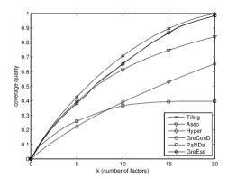
(a) Set 1

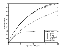
(b) Set 2

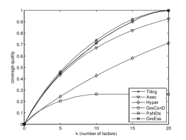
(c) Set 3

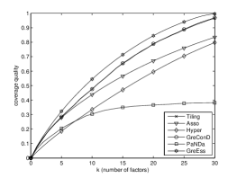
(d) Set 4

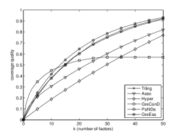
(e) Set 5

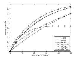
(f) Set 6

Figure 1: Coverage quality of the first $k$ factors (synthetic data).

		coverage $c$ of the first $k$ factors
dataset	$k$	Tiling	Asso	Hyper	GreConD	PaNDa	GreEss
Set 1	5	0.3820	0.3929	0.2234	0.3820	0.2586	0.4260
	10	0.6557	0.6131	0.3894	0.6512	0.3654	0.7068
	15	0.8645	0.7467	0.5294	0.8686	0.3925	0.8957
	20	0.9839	0.8387	0.6529	0.9852	0.3958	0.9971
	25	1.0000	0.9049	0.7602	1.0000	0.3958	1.0000
Set 2	5	0.4970	0.4919	0.3187	0.4961	0.2591	0.5035
	10	0.7755	0.7594	0.5326	0.7764	0.2864	0.7764
	15	0.9326	0.9141	0.6850	0.9330	0.2933	0.9418
	20	1.0000	0.9894	0.8139	0.9982	0.2933	1.0000
	25	1.0000	0.9977	0.9090	1.0000	0.2933	1.0000
Set 3	5	0.4471	0.4341	0.2435	0.4485	0.2041	0.4620
	10	0.7114	0.6725	0.4268	0.7163	0.2647	0.7384
	15	0.9011	0.8246	0.5814	0.9011	0.2647	0.9219
	20	0.9980	0.9259	0.7136	1.0000	0.2647	0.9991
	25	1.0000	0.9812	0.8176	1.0000	0.2647	1.0000
Set 4	5	0.2822	0.2794	0.1849	0.2851	0.2047	0.3228
	10	0.4760	0.4379	0.3352	0.4761	0.3039	0.5450
	20	0.7869	0.6711	0.5953	0.7894	0.3661	0.8450
	30	0.9655	0.8344	0.7978	0.9698	0.3820	0.9969
	40	1.0000	0.9381	0.9414	1.0000	0.3824	1.0000
Set 5	5	0.2251	0.2095	0.0984	0.2203	0.3471	0.2471
	15	0.5053	0.3873	0.2729	0.4983	0.5034	0.5455
	30	0.7471	0.6021	0.5050	0.7575	0.5706	0.7871
	50	0.9154	0.8206	0.7712	0.9234	0.5706	0.9319
	60	0.9577	0.8867	0.8830	0.9652	0.5706	0.9666
Set 6	5	0.2004	0.1817	0.1096	0.2110	0.2592	0.2443
	15	0.4779	0.3666	0.2980	0.4841	0.4253	0.5391
	30	0.7462	0.5851	0.5439	0.7396	0.5290	0.7980
	50	0.9310	0.7978	0.8069	0.9281	0.5368	0.9552
	60	0.9752	0.8716	0.9079	0.9734	0.5368	1.0000

Table 4: Quality of decompositions (synthetic data).

	coverage	number of factors needed for the prescribed coverage
dataset	($100c\%$)	Tiling	Asso	Hyper	GreConD	PaNDa	GreEss
Mushroom	25%	3	2	8	3	1	2
	50%	7	6	19	7	NA	8
	75%	24	36	37	24	NA	26
	100%	119	NA	122	120	NA	105
DBLP	25%	2	2	2	2	NA	2
	50%	5	5	5	5	NA	5
	75%	10	10	10	11	NA	10
	100%	21	19	19	20	NA	19
Paleo	25%	16	16	14	16	NA	15
	50%	39	40	38	39	NA	38
	75%	75	76	73	76	NA	73
	100%	151	NA	139	152	NA	145
Chess	25%	2	1	9	1	1	1
	50%	5	2	26	4	NA	6
	75%	16	15	39	15	NA	17
	100%	124	NA	90	124	NA	113
DNA	25%	8	6	24	8	NA	13
	50%	32	27	67	33	NA	41
	75%	94	80	155	96	NA	105
	100%	489	NA	392	496	NA	408
Tic-tac-toe	25%	5	6	5	5	NA	5
	50%	12	12	11	12	NA	12
	75%	19	19	18	19	NA	19
	100%	31	29	29	32	NA	32

Table 5: Quality of decompositions (real data).

All the algorithms compute the factors for a given $I$ one after another. In case of Tiling, Hyper, GreConD and GreEss, this process is guaranteed to stop when an exact decomposition $I=A\circ B$ is found. With Asso and PaNDa, it often happens that an exact decomposition is not found and that the algorithm stops with a relatively small coverage $c$ (i.e. large error $E(I,A\circ B)$), which is seen from the tables and graphs and is indicated by NA in Table 5. This is in particular true of PaNDa. This feature, which is a consequence of committing the error $E_{o}$ (cf. Observation 2 and the discussion below), is a disadvantage of Asso and PaNDa when a large coverage is required. On the other hand, Asso tends to have a good coverage by the first couple of factors. Asso performs better on datasets which are sparse or dense compared to other datasets, which can be observed on Set 2 and Set 5. PaNDa tends to have a good coverage by the first couple of factors on dense datasets which is seen in case of Set $5$. Hyper performs well with respect to the first quality criterion, namely the total number of factors needed for an exact decomposition of the input matrix. For the synthetic datasets, Hyper is the fourth best, behind Tiling, GreConD, and GreEss, with GreEss being the best one. For the six real datasets, Hyper  is comparable to GreEss in terms of the first quality criterion. However, Tables 4 and 5 and the slowly-growing curves of coverage quality in Fig. 1 reveal a significant drawback of Hyper, namely a poor coverage by the set of the first $k$ factors, even for a relatively large $k$. The reason for this behavior is the following. Hyper includes in the set $\mathcal{C}_{\alpha}$ (see the above description of Hyper) not only the rectangles corresponding to $\alpha$-frequent itemsets but also those corresponding to all the singleton itemsets. Including the singleton itemsets guarantees that an exact decomposition of the input matrix is found when Hyper computes them from $\mathcal{C}_{\alpha}$. It turns out from the results, however, that the factors corresponding to the singleton items, i.e. the rectangles induced by the columns of the input matrix are used very often. This causes a very low coverage by the sets of the first $k$ factors of Hyper compared to the other algorithms. Note in this connection that a trivial factorization algorithm that outputs for an input matrix $I\in\{0,1\}^{n\times m}$ the set $\mathcal{F}$ containing the $m$ rectangles corresponding to the columns of $I$ will have a similar behavior in a sense, namely a slowly-growing curve of coverage quality which, nevertheless, reaches full coverage (exact decomposition) with $k\leq m$. None of Tiling, GreConD, and GreEss suffers from this drawback of Hyper. Tiling and GreConD perform very similarly, confirming the evaluation results of Algorithm 1 and GreConD in [4] (cf. the description of GreConD above). One can see from the results that GreEss performs best of these three algorithms on both synthetic and real datasets, outperforming them significantly, particularly in terms of the number of factors needed for exact decomposition.

From the point of view of the new strategy of GreEss, which is based on the results regarding essential part of $I$, the following conclusions may be drawn. Contrary to Tiling, Asso, Hyper, GreConD and PaNDa, which all use different strategies of greedy coverage, but all aim at covering the most of the uncovered $1$s in $I$, GreEss proceeds differently. In its greedy coverage, GreEss focuses on the essential $1$s in $I$ and considers them as “seeds” of good factors. Such strategy is theoretically well justified, is fast, and leads to improvement in quality of Boolean matrix factorization.

5.4 Performance on Synthetic Data With Noise

Noise in Boolean data is an issue discussed in the papers on BMF, see e.g. [21, 16]. In particular, PaNDa has been designed with the aim to perform well for data with noise. The capability to factorize noisy data with Asso has been demonstrated in [21]. In this section we provide the performance evaluation of GreEss for noisy data and compare it with Asso and PaNDa. We use a scenario similar to those of [21, 16]. We performed the evaluation on synthetic datasets which are obtained by adding noise to the datasets generated as those comprising Sets $1,\dots,6$ in Section 5.1. In particular, we display the results for the datasets obtained by the same parameters as those for Set $2$. The results are similar for the other parameters.

We observed the coverage quality of the datasets in a similar way as in Section 5.3. The results are displayed in Figure 2.

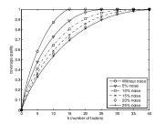
(a) Aditive noise—GreEss

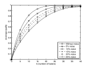
(b) Aditive noise—Asso

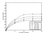
(c) Aditive noise—PaNDa

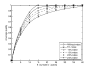
(d) Substractive noise—GreEss

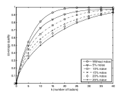
(e) Substractive noise—Asso

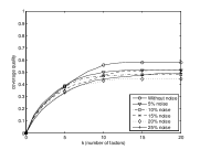
(f) Substractive noise—PaNDa

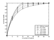
(g) General noise—GreEss

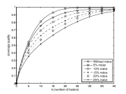
(h) General noise—Asso

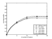
(i) General noise—PaNDa

Figure 2: Coverage quality of the first $k$ factors (synthetic data with noise).

For each of the algorithms we provide results for additive noise, subtractive noise, and general noise, and for every type of noise we include six levels of noise, from 0% to 25%. Adding additive noise of $p\%$ to a Boolean matrix $I$ means that we flip at random with probability $p$ the entries in $I$ containing $0$ (change $0$ to $1$). For subtractive noise, we flip the entries containing $1$ and for general noise we flip at random all the entries. The curves represent the coverage quality by the sets of the first $k$ factors computed by the algorithms as in Section 5.3. That is, the values for each curve are obtained as averages over 1000 particular datasets with the respective level of noise. We can see in Figure 2 that all the algorithms share the property that as the level of noise increases, the curve of the coverage quality gets shifted down, i.e. a larger number of factors is needed to explain a given portion of data. A possible interpretation of the observed shifts is that the larger the shift, the more sensitive the particular algorithm is for the particular type of noise. In the context of the current view, according to which using only factors that are not allowed to cover the entries of $I$ containing $0$ leads to sensitivity to noise, the graphs show a somewhat surprising fact. Namely, the sensitivity to noise in the above sense for GreEss, which uses only such factors covering $1$s, turns out not to be larger than for Asso and PaNDa. On the other hand, we believe that the current view of noise and sensitivity to noise in BMF is limited and that the problem of noise needs a solid foundation. For example, a natural question is whether and to what extent it is the case that if a particular algorithm discovers good factors in a given data, then when noise is added, the algorithm still discovers these or similar factors. This question needs to be considered with care because adding significant amount of noise, as in case of some experiments in the literature on BMF, may change the data to the extent that it is much better explained by new, previously absent factors.

6 Conclusions

We presented new results on BMF that are based on examining the closure and order-theoretic structures related to Boolean data. The results let us differentiate the role of entries of the input matrix and suggest where to focus in computing decompositions. We proposed a new BMF algorithm, GreEss, based on these results and provided results of its experimental evaluation. It turns out that the algorithm performs well both in terms of coverage of the input data by the first $k$ factors (i.e. by a small number of the most important factors) and in terms of the number of factors needed for an exact decomposition of the input matrix (i.e. factors that fully explain the input data) and that GreEss outperforms the existing algorithms. The presented results, both theoretical and experimental, emphasize the role of from-below factorization algorithms in BMF, of which GreEss is an example.

An important topic for future research is to utilize further the present results regarding essential parts of Boolean matrices and to further investigate the role of entries of Boolean matrices for BMF. In particular, it seems promising to explore the possibility to still reduce $\mathcal{E}(I)$ to $\mathcal{E}(\mathcal{E}(I))$, and in general, to $\mathcal{E}^{p}(I)$. Furthermore, the notion of $\varepsilon$-essential part shall be investigated for $\varepsilon>0$. Another topic is to utilize as heuristics other information that may be obtained from the intervals $\mathcal{I}_{ij}$, in particular the number $|\mathcal{I}_{ij}|$ of concepts covering $\langle i,j\rangle$. This number is difficult to compute but our preliminary results indicate that it may be approximated quickly. Note that the case $|\mathcal{I}_{ij}|=1$ corresponds to so-called mandatory factors considered in [4], i.e. factors that need to be present in every exact decomposition of $I$. An important topic is to extend the theoretical framework to general factorizations involving rectangles containing possibly $0$s, which are sometimes called fault-tolerant concepts or noisy tiles, see e.g. [5]. An interesting goal is to extend the present results beyond Boolean data, namely to ordinal and semiring-valued data, see e.g. [2] for general results on closure structures and decompositions of such, more general data. Last but not least, let us mention that three- and multi-way data received a considerable attention recently. [3, 19] present approaches to factorization of three-way Boolean data. An extension of the present results to multi-way data seems another important research topic.

References

- [1] Bache K., Lichman M., UCI Machine Learning Repository [http://archive.ics.uci.edu/ml], Irvine, CA: University of California, School of Information and Computer Science, 2013.
- [2] Belohlavek R., Optimal decompositions of matrices with entries from residuated lattices, J. Logic Comput. 22(6)(2012), 1405–1425.
- [3] Belohlavek R., Glodeanu C., Vychodil V., Optimal factorization of three-way binary data using triadic concepts, Order 30(2)(2013), 437–454 (preliminary version in Proc. GrC 2010).
- [4] Belohlavek R., Vychodil V., Discovery of optimal factors in binary data via a novel method of matrix decomposition, J. Comput. Syst. Sci. 76(1)(2010), 3–20 (preliminary version in Proc. SCIS & ISCIS 2006).
- [5] Besson J., Pensa R.G., Robardet C., Boulicaut J.F., Constraint-based mining of fault-tolerant patterns from Boolean data, Proc. KDID 2006, pp. 55–71.
- [6] Brualdi R. A., Ryser H. J., Combinatorial Matrix Theory, Cambridge University Press, 1991.
- [7] Davey B. A., Priestley H. A., Introduction to Lattices and Order (2nd ed.). Cambridge University Press, 2002.
- [8] Ganter B., Glodeanu C. V., Ordinal Factor Analysis, Lecture Notes in Computer Science 7278(2012), 128–139.
- [9] Ganter B., Wille R., Formal Concept Analysis: Mathematical Foundations, Springer, Berlin, 1999.
- [10] Geerts F., Goethals B., Mielikäinen T., Tiling databases, Proc. Discovery Science 2004, pp. 278–289.
- [11] Kim K.H., Boolean Matrix Theory and Applications, M. Dekker, NY, 1982.
- [12] Kontonasios K.-N., De Bie T., An information-theoretic approach to finding informative noisy tiles in binary databases, SIAM DM 2010, pp. 153–164.
- [13] Kuznetsov S.O., Obiedkov S., Comparing performance of algorithms for generating concept lattices, J. Exp. and Theor. Artif. Intell. 14(2002), 189–216.
- [14] Lu H., Vaidya J., Atluri V., Optimal Boolean matrix decomposition: application to role engineering, Proc. IEEE ICDE 2008, pp. 297–30.
- [15] Lu H., Vaidya J., Atluri V., Hong Y., Constraint-aware role mining via extended Boolean matrix decomposition, IEEE Trans. Dependable and Secure Comp. 9(5)(2012), 655–669.
- [16] Lucchese C., Orlando S., Perego R., Mining top-K patterns from binary datasets in presence of noise, SIAM DM 2010, pp. 165–176.
- [17] Miettinen P., The Boolean column and column-row matrix decompositions, Data Mining and Knowledge Discovery 17(2008), 39–56.
- [18] Miettinen P., Sparse Boolean matrix factorizations, Proc. IEEE ICDM 2010, pp. 935–940.
- [19] Miettinen P., Boolean tensor factorizations, Proc. IEEE ICDM 2011, pp. 447–456.
- [20] Miettinen P., On finding joint subspace Boolean matrix factorizations, SDM 2012, pp. 954–965.
- [21] Miettinen P., Mielikäinen T., Gionis A., Das G., Mannila H., The discrete basis problem, IEEE Trans. Knowledge and Data Eng. 20(10)(2008), 1348–1362 (preliminary version in Proc. PKDD 2006).
- [22] Miettinen P., Vreeken J., Model order selection for Boolean matrix factorization, Proc. ACM SIGKDD 2011, pp. 51–59.
- [23] Monson S. D., Pullman S., Rees R., A survey of clique and biclique coverings and factorizations of (0,1)-matrices, Bull. ICA 14(1995), 17–86.
- [24] Myllykangas S. et al, 2006, DNA copy number amplification profiling of human neoplasms, Oncogene 25(55)(2006), 7324–7332.
- [25] Nau D.S., Specificity covering, Tech. Rep. CS-1976-7, Duke University, 1976.
- [26] Nau D.S., Markowsky G., Woodbury M.A., Amos D.B., A mathematical analysis of human leukocyte antigen serology, Math. Biosci. 40(1978), 243–270.
- [27] Outrata J., Boolean factor analysis for data preprocessing in machine learning, Proc. ICMLA 2010, pp. 899–902.
- [28] Schmidt G., Relational Mathematics, Cambridge University Press, 2011.
- [29] Stockmeyer L., The set basis problem is NP-complete, Tech. Rep. RC5431, IBM, Yorktown Heights, NY, USA, 1975.
- [30] Tatti N., Vreeken J., Comparing apples and oranges: measuring differences between exploratory data mining results, Data Mining and Knowledge Discovery 25(2012), 173–207 (preliminary version in Proc. ECMLPKDD 2011).
- [31] Tatti N., Mielikäinen T., Gionis A., Mannila H., What is the dimension of your binary data?, Proc. IEEE ICDM 2006, pp. 603–612.
- [32] Vaidya J., Atluri V., Guo Q., The role mining problem: finding a minimal descriptive set of roles, Proc. SACMAT 2007, pp. 175–184.
- [33] Xiang Y., Jin R., Fuhry D., Dragan F. F., Summarizing transactional databases with overlapped hyperrectangles, Data Mining and Knowledge Discovery 23(2011), 215–251 (preliminary version in Proc. ACM KDD 2008).