A Physical-layer Rateless Code for Wireless Channels

Abstract

In this paper, we propose a physical-layer rateless code for wireless channels. A novel rateless encoding scheme is developed to overcome the high error floor problem caused by the low-density generator matrix (LDGM)-like encoding scheme in conventional rateless codes. This is achieved by providing each symbol with approximately equal protection in the encoding process. An extrinsic information transfer (EXIT) chart based optimization approach is proposed to obtain a robust check node degree distribution, which can achieve near-capacity performances for a wide range of signal to noise ratios (SNR). Simulation results show that, under the same channel conditions and transmission overheads, the bit-error-rate (BER) performance of the proposed scheme considerably outperforms the existing rateless codes in additive white Gaussian noise (AWGN) channels, particularly at low BER regions.

I Introduction

Rateless codes [1] were initially developed to achieve efficient transmission in erasure channels. The Luby transform (LT) code [2] is broadly viewed as the first practical realization of rateless codes. The LT encoded symbols are generated in accordance with a specific degree distribution and there is potentially an unlimited number of encoded symbols. These symbols are generated on the fly and broadcasted to the receiver until an acknowledgment (ACK) response of successful decoding is received at the transmitter.

Ideally, a rateless code should allow the receiver to recover the message symbols with high probability by receiving as few encoded symbols as possible. Aiming to reduce the necessary number of encoded symbols, Shokrollahi proposed Raptor codes in [3]. In Raptor codes, a precoding (e.g., based on low-density parity-check (LDPC) codes) is applied to the message symbols prior to the LT code. In [3], Raptor codes are constructed in systematic and non-systematic manners for different erasure channel scenarios.

The initial work on rateless codes has mainly been limited to erasure channels with the primary application in multimedia video streaming. Recently, the design of rateless codes for wireless channels, such as binary symmetric channels (BSC) [4], additive white Gaussian noise (AWGN) channels [5], [6], as well as fading channels [7], has attracted significant attention. Rateless codes have a wide spectrum of applications in various modern wireless communication networks, such as to enhance the transmission efficiency in IEEE ad-hoc 802.11b wireless networks [8] and cooperative relay networks [9], [10], and to control the peak-to-average power ratio in OFDM systems [11]. Rateless codes are particularly beneficial to wireless transmissions because, in contrast to traditional fixed-rate coding schemes, the transmitter potentially does not need to know the channel state information before sending its encoded symbols, and the receiver can retain a resilient decoding performance. This property is of particular importance in the design of codes for time varying wireless channels.

In general, there are two categories of physical-layer rateless codes for wireless channels: systematic [8], [12] and non-systematic [6], [13], [14], [15]. For systematic rateless codes, the systematic message symbols are first transmitted to the receiver, followed by a number of encoded symbols. For non-systematic rateless codes, only encoded symbols are broadcasted. The receiver uses the classic belief propagation (BP) algorithm for decoding [16]. At the transmitter, the encoder of the existing rateless codes uses coding schemes that are akin to the low-density generator matrix (LDGM) codes [17]. The LDGM-like rateless codes are of linear complexity for encoding and their encoded symbols can be simply calculated on the fly.

A major drawback of the existing physical-layer rateless codes is the notably high error floor. This error floor is present mainly because, from the BP decoding perspective, the encoder creates an encoded symbol by selecting systematic message symbols only. As a result, the encoded symbol is connected to only one check node and cannot receive updated information as the decoding progresses. Therefore, an erroneous encoded symbol keeps propagating the error message through its corresponding check node to the systematic message symbols, which are connected to that check node. To improve the error floor performance, a considerable amount of research has been conducted in the past several years, which can be broadly divided into two directions. One direction applies serial concatenated coding schemes [13], [14], [18], where the LDGM-like rateless code is used as a component code in the concatenation structure. The other direction modifies the LDGM-like rateless code as a stand-alone code without concatenation [6], [15]. As reported in [6], the error performance of concatenation codes is largely determined by the stand-alone rateless code itself, and the concatenation will inevitably increase the system complexity. Therefore, in this paper, we will focus on the design of the stand-alone rateless code. In [15] and [19], it shows that the error floor in LDGM-like codes is closely related to the systematic message symbols connected to a relatively small number of check nodes. The error floor can be reduced to a certain level by reducing the number of message symbols of a lower-degree. For this purpose, [15] proposed to connect all message symbols to an approximately equal number of check nodes. However, the method in [15] suffers from a high error floor problem especially at low signal to noise ratio (SNR) regime. This is because all encoded symbols still have degree-one, and thus cannot receive updated information from other check nodes in the BP decoder.

Another major drawback of the existing physical-layer rateless codes is that different wireless channel conditions need different check node degree distributions to achieve the near-capacity performance [6]. This is primarily because, for the LDGM-like rateless codes, the degree of systematic message symbols continues to increase as the transmission goes on to generate and transmit more encoded symbols. From the extrinsic information transfer (EXIT) chart perspective [20], increasing the degree of systematic message symbols will change the EXIT curve of variable nodes. To achieve a low bit-error-rate (BER) for a near-capacity transmission overhead, an open but minimum spacing EXIT chart tunnel is required. As a result, the inverted EXIT curve of check nodes needs to follow the change, which in turn causes the check node degree distribution to change. Obviously, to utilize multiple distributions and adjust them to fit different channel conditions would complicate the transmission mechanism. A robust check node degree distribution that can perform well over a wide range of SNRs would dramatically simplify the system. Some initial studies [14], [21] have attempted to design a robust degree distribution, but the progress has been limited so far.

In this paper, we first develop a rateless encoding approach to resolve the high error floor problem caused by the conventional LDGM-like rateless encoding schemes in wireless channels. For the proposed approach, the encoder creates an encoded symbol by selecting not only the systematic message symbols, but also the encoded symbols created prior to the present encoded symbol. By doing so, each encoded symbol will be connected to multiple check nodes in the Tanner graph [22]. Moreover, to provide all the symbols with approximately equal protection in the BP decoder, we require each variable node to connect to an approximately equal number of check nodes. To achieve this, we let the variable nodes with a lower degree be selected with a higher priority when the encoder selects variable nodes for each check equation to form an encoded symbol. By using the proposed encoding approach, the encoded symbol can exchange information with other symbols through multiple check nodes as the decoding progresses. As a result, the error floor is lowered.

To provide satisfactory performance over a wide range of SNRs, we develop an EXIT-chart-based optimization approach and achieve a near optimal robust check node degree distribution for the proposed rateless code. This robust distribution is able to create a constant EXIT chart tunnel for different SNRs. In general, for the conventional rateless codes under a particular channel condition, the shape of the EXIT curve of variable nodes is determined by the variable node degree distribution. This distribution depends on two factors: one is the check node degree distribution, and the other is the number of symbols transmitted [6]. To achieve a satisfactory decoding performance, the lower the SNR is, the more symbols need to be transmitted. Therefore, when SNR changes, the EXIT curve inevitably changes. In contrast, for the proposed rateless code, we can keep the EXIT curve unchanged by dividing the variable nodes involved in the BP decoder into two sets and manipulating the sizes of the two sets. One set corresponds to the received symbol sequence from the wireless channel. This received sequence consists of all the encoded symbols and the message symbols that are actually transmitted. The other set of variable nodes corresponds to the remaining message symbols that are yet to be transmitted. We adjust the number of message symbols in the two sets in order to achieve a stable EXIT curve of variable nodes for a desired range of SNRs. Consequently, we can achieve a well-behaved and constant EXIT chart tunnel leading to superior performances. Simulation results show that, under the same channel condition and transmission overhead, the BER performance of the proposed code considerably outperforms the existing rateless codes in additive white Gaussian noise (AWGN) channels, particularly at low BER regions.

The rest of the paper is organized as follows. In Section II, the system model is introduced. In Section III, the conventional rateless codes are discussed. In Section IV, the construction of the proposed rateless code is described first, followed by a discussion of optimizing the check node degree distribution based on the EXIT chart analysis. Simulation results are presented in Section V. Some concluding remarks are made in Section VI.

II System Model

In this paper, we consider a point-to-point physical-layer transmission in AWGN channels. The system model is shown in Fig. 1. Let $\textbf{b}=\{b_{1},...,b_{j},...,b_{K}\}$ denote the binary message symbols, generated by the source, where $b_{j}$ is the $j$-th symbol and $K$ is the length of message. The message symbols are first encoded by a rateless channel encoder. Let $v_{t}$ represent the $t$-th binary rateless coded symbol, which is then modulated and transmitted. We consider the binary phase shift keying (BPSK) modulation. Let $x_{t}\in\{+1,-1\}$ be the modulated signal of $v_{t}$. The received signal, $y_{t}$, at the receiver is given by

$$y_{t}=\sqrt{P_{T}}x_{t}+n_{t}$$ (1)

where $P_{T}$ is the transmission power, which is assumed to be of unity power, i.e. $P_{T}=1$, and $n_{t}$ is the real-valued additive noise in AWGN channels with zero-mean and variance of $\sigma_{n}^{2}$. After receiving the rateless coded symbols, the receiver applies the BP decoding algorithm [16] to recover the source message. For the rateless code, the encoder generates an unlimited number of symbols and keeps transmitting these symbols until it receives an ACK response from the receiver.

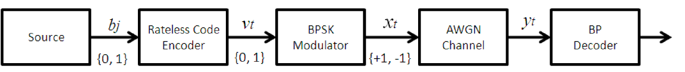
Figure 1: The considered digital communication system model

III Conventional Physical-layer Rateless Codes

In the encoding phase, the encoder first draws a value of $d$ from a distribution called the check node degree distribution. The encoder then randomly selects $d$ systematic message symbols, and performs binary summation (i.e. XOR) of these selected symbols to generate an encoded symbol. The relationship of systematic message symbols and encoded symbols can be represented by a bipartite Tanner graph [22]. Fig. 2 shows the Tanner graph of the conventional LDGM-like rateless codes. In the Tanner graph, the systematic message symbols are denoted by ‘$\bigcirc$’ and the encoded symbols by ‘$\square$’. The vertices ‘$\blacksquare$’ are check nodes representing the parity-check equation constraint.

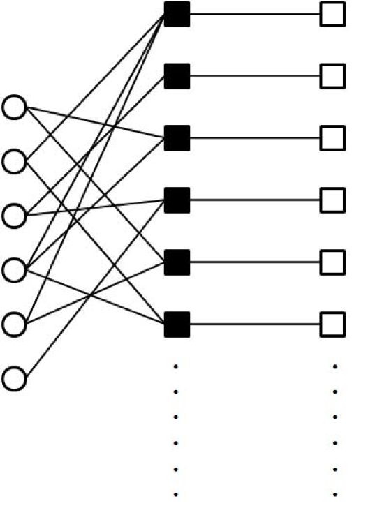
Figure 2: The Tanner graph representing an instance of a systematic LDGM code [17]. ‘$\bigcirc$’ represents the systematic message symbols, ‘$\square$’ the encoded symbols and ‘$\blacksquare$’ the check nodes.

At the receiver, to evaluate the BER performance of the rateless codes in AWGN channels, Etesami and Shokrollahi introduced a formal definition of the reception overhead $\delta$ of a decoder in [6]. Let $M$ denote the number of binary symbols collected at the receiver to perform satisfactory decoding in the BP decoder. We express $M$ as

$$M=\frac{K}{C_{\sigma_{n}}}(1+\delta)$$ (2)

where $C_{\sigma_{n}}$ is the achievable code rate for binary-input continuous-output AWGN channels with the noise level parameter $\sigma_{n}$. This noise level $\sigma_{n}$ is often called the Shannon limit. From (2), we can see that the overhead $\delta$ represents the number of collected binary symbols away from the optimal number defined by $K/C_{\sigma_{n}}$.

For equiprobable $x_{t}\in\{+1,-1\}$, $C_{\sigma_{n}}$ is given by [23]

$$C_{\sigma_{n}}=-\int_{-\infty}^{\infty}\phi_{\sigma_{n}}(y)\log_{2}\phi_{\sigma_{n}}(y)dy-\frac{1}{2}\log_{2}2\pi e\sigma_{n}^{2}$$ (3)

where

$$\begin{split}&\phi_{\sigma_{n}}(y)=\\ &\frac{1}{\sqrt{8\pi\sigma_{n}^{2}}}\left(\exp\left(-\frac{(y+1)^{2}}{2\sigma_{n}^{2}}\right)+\exp\left(-\frac{(y-1)^{2}}{2\sigma_{n}^{2}}\right)\right)\,.\end{split}$$ (4)

Since there is no closed form expression, the integral in (3) is evaluated by numerical integration techniques [24]. Table I and Fig. 3 show the Shannon limits as a function of some specific code rates $R$. These values will be used later for the design of the proposed rateless code. The last column in Table I is the Shannon limit expressed as the ratio (dB) of signal energy per symbol to noise power spectral density, and is defined as

$$\frac{E_{b}}{N_{0}}=10\log_{10}\left(\frac{1}{2R\sigma_{n}^{2}}\right)\,.$$ (5)

$R$	$\sigma_{n}$	$\frac{E_{b}}{N_{0}}\,\textrm{(dB)}$
0.501	0.977	0.1934
0.912	0.5	3.4104
0.999	0.2859	7.864

TABLE I: Shannon limits for various code rates $R$.

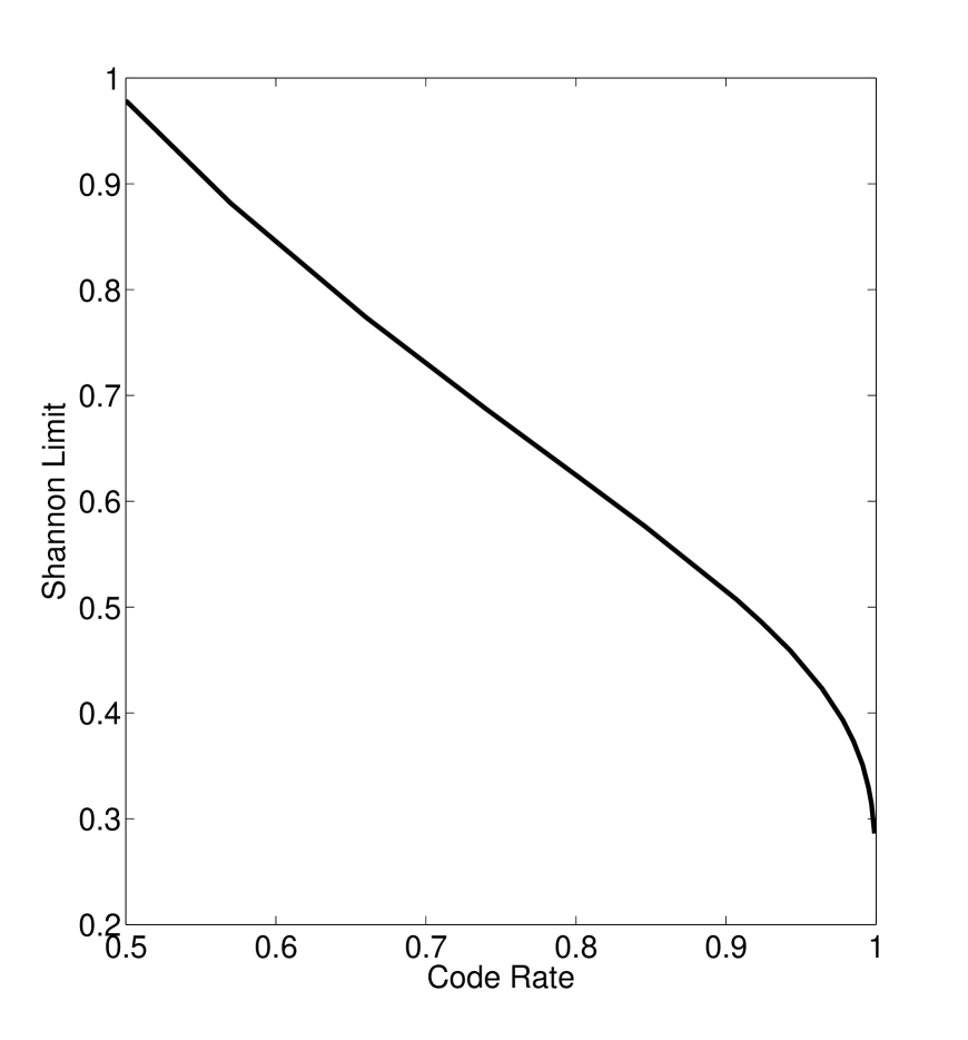
Figure 3: Shannon Limit $\sigma_{n}$ vs. Code Rate $R$

IV Proposed Physical-layer Rateless Codes Scheme

In this section, the construction of the proposed rateless code is described first. A ball-into-bin method is developed to have the encoded symbol connected to multiple check nodes, and a full rank parity-check matrix tailored to the transmission characteristics of wireless channels is constructed. The EXIT-chart-based optimization program is then employed to optimize the robust check node degree distribution.

IV-A Construction of the Proposed Coding Scheme

To overcome the high error floor problem in the LDGM-like encoding scheme, we propose a rateless coding scheme where the encoder generates an encoded symbol by using not only the systematic message symbols, but also the encoded symbols created before the present one. Each encoded symbol will be connected to multiple check nodes (check equations). Through these check nodes, each variable node and check node can exchange information with other nodes as the BP decoding progresses. In this way, the error floor can be lowered considerably.

Let us look at a simple example in Fig. 4, which illustrates the proposed encoding representation by using a Tanner graph. In this example, the number of systematic message symbols $K=6$. The set of vertices on the left is called variable nodes, representing the systematic message symbols ‘$\bigcirc$’ and the encoded symbols ‘$\square$’. The vertices ‘$\blacksquare$’ on the right are check nodes. Since each encoded symbol is generated by a check equation, each variable node corresponding to an encoded symbol is connected to its corresponding check node (check equation) in the graph.

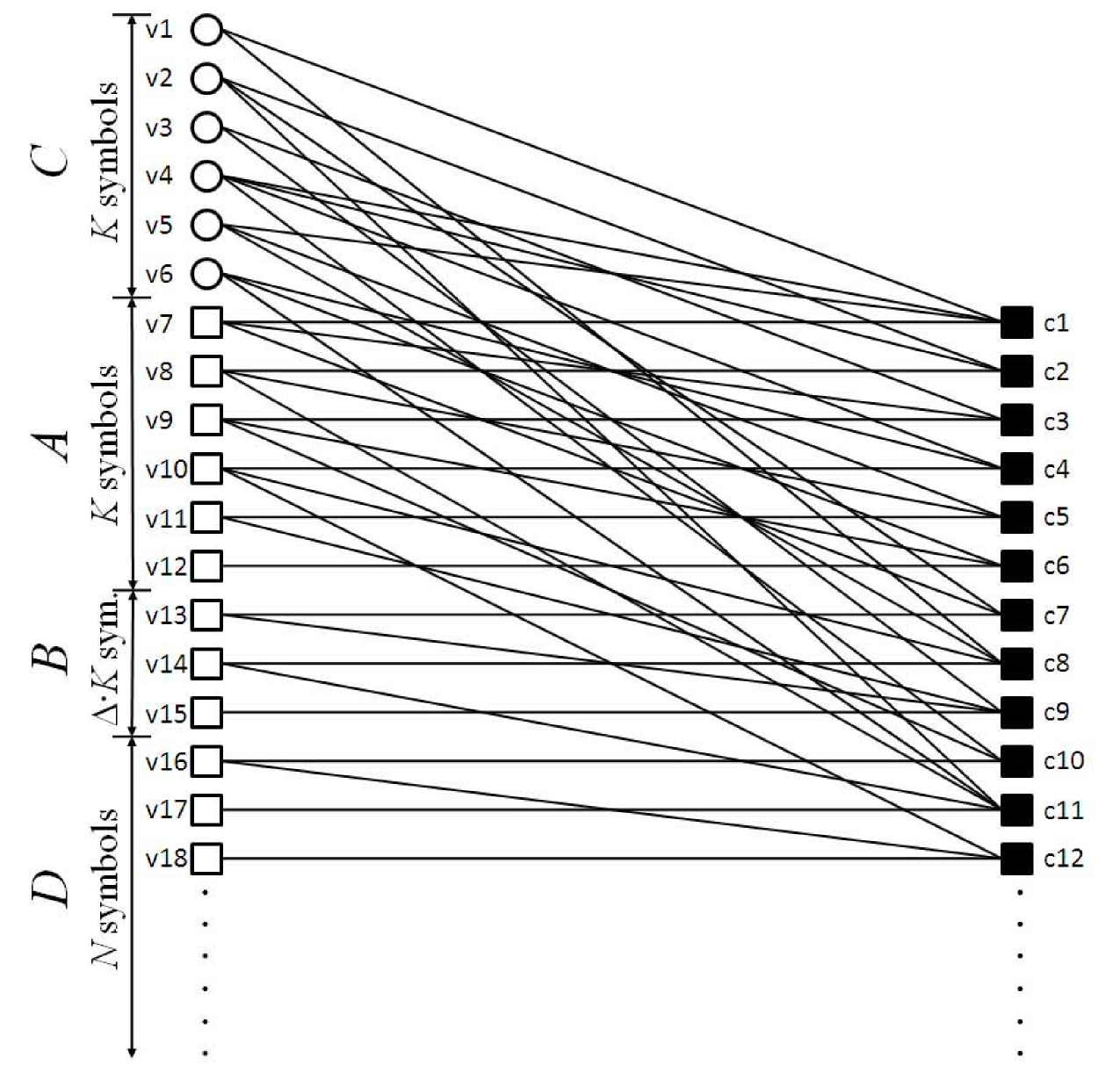
Figure 4: The Tanner graph representing an instance of the proposed rateless code. ‘$\bigcirc$’ represents the systematic message symbols, ‘$\square$’ the encoded symbols and ‘$\blacksquare$’ the check nodes.

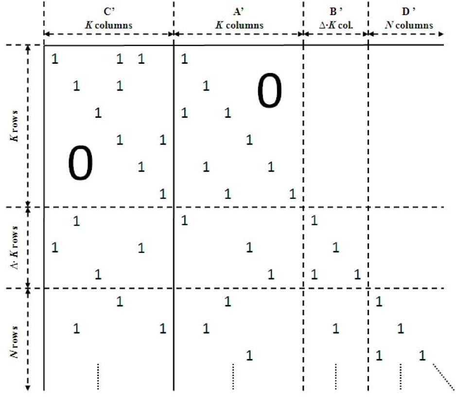
Figure 5: The parity-check matrix representing the instance of the proposed rateless code in Fig. 4

An ideal rateless code commonly requires a check node to be randomly connected to variable nodes. For a check node of degree $i$ in the LT-based encoding schemes, the check node selects $i-1$ systematic message symbols in a uniformly random manner to produce an encoded symbol as shown in Fig. 2. This implies that the degree of the message symbols, or in other words, the number of check nodes a message symbol connects to, can be very broadly distributed. Some of the message symbols may not even have a connection to any check node unless a sufficiently large number of check nodes are provided. Consequently, even for very high SNRs, there is still a great chance that the decoding error would occur due to the unconnected message symbols. Thus, from the transmission efficiency point of view, a completely random selection would not be suitable for high SNR regions in AWGN channels. To boost the transmission efficiency at high SNRs, we apply a full rank constraint to the parity-check matrix H of the proposed rateless code. The structure of H of the code in Fig. 4 is shown in Fig. 5. Each row of H corresponds to a parity-check equation and each column of H corresponds to a symbol in the rateless code. We decompose H into two parts. The first part of H corresponds to the encoded symbols and consists of the ($K+1$)-th to the rightmost columns of H. This part is a sparse lower triangular matrix. The second part of H corresponds to the $K$ message symbols and consists of the first $K$ columns of H. In the second part, a sparse upper triangular matrix is on top of a regular sparse matrix. The purpose of producing the upper triangular matrix is to guarantee a full rank matrix for the first $K$ rows of H. This full rank design ensures that when SNR is sufficiently high, even though none of the message symbols are transmitted, all message symbols can be successfully decoded as soon as the decoder receives the first $K$ encoded symbols. When SNR is lowered, more symbols have to be transmitted to achieve satisfactory decoding performance. In this case, we require all the variable nodes to connect to an approximately equal number of check nodes, which ensures that all transmitted symbols receive almost the same protection from the BP decoder. In the following, a ball-into-bin encoding scheme is developed to construct a rateless code as discussed above.

$\blacklozenge$ Ball-into-bin encoding procedure: to better describe the encoding process, let us first look at an example with $K=6$. Suppose there are $K+L$ ‘variable balls’, $v_{1},\dots,v_{K+L}$, corresponding to $K+L$ variable nodes. As shown in Fig. 6, these variable balls are classified into two groups. The first group, which we call the systematic ball group, includes balls, $v_{1},\dots,v_{K}$, representing the $K$ systematic binary message symbols. The second group, which we call the encoded ball group, contains balls, $v_{K+1},\dots,v_{K+L}$, representing the $L$ encoded symbols, and the values for these encoded symbols are to be determined in the encoding process. Let $\Omega_{i}$ denote the check node degree distribution, where $i=1,2,\dots,i_{max}$. $\Omega_{i}$ represents the probability that a check node has degree $i$, and $i_{max}$ is the maximum check node degree. Similarly, we denote by $d_{max}$ the maximum variable node degree. There are $d_{max}+1$ degree bins labeled as ‘Bin of Degree $0$’, ‘Bin of Degree $1$’, ‘Bin of Degree $2$’, …, ‘Bin of Degree $d_{max}$’. A ball $v_{j}$ sitting in ‘Bin of Degree $d$’ means that $v_{j}$ is of degree $d$ and has connections to $d$ check nodes. We also introduce a bin labeled as ‘Buffer Bin’ to produce the upper triangular matrix in H. Only systematic balls can be put into ‘Buffer Bin’ by the encoder. If a ball is put into ‘Buffer Bin’, it will not be used to generate encoded symbols unless drawn out of ‘Buffer Bin’ and put into the degree bins. The detailed application of the ‘Buffer Bin’ will be described later in this section. In addition, since there are $L$ encoded symbols, we have $L$ check nodes, $c_{1},\dots,c_{L}$ in Fig. 6, correspondingly.

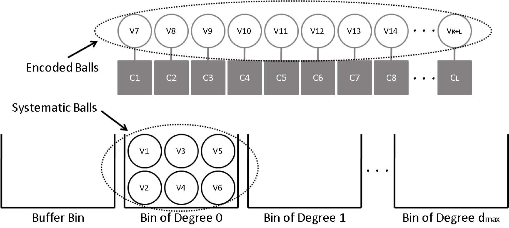
Figure 6: An instance of the ball-into-bin encoding process for $l=0$. ‘$\bigcirc$’ represents the variable balls and ‘$\blacksquare$’ the check nodes. ($K=6$)

Denoting by $l$ the index of the check nodes, the encoding procedure progresses as $l$ increases from one to $L$, and is divided into two phases. Phase I, $1\leq l\leq K$, will generate the first $K$ encoded symbols, which will form the upper triangular matrix of H; Phase II, $K+1\leq l\leq L$, will generate the rest $L-K$ encoded symbols. Before the encoding process begins ($l=0$, Fig. 6), all systematic balls sit in ‘Bin of Degree $0$’.

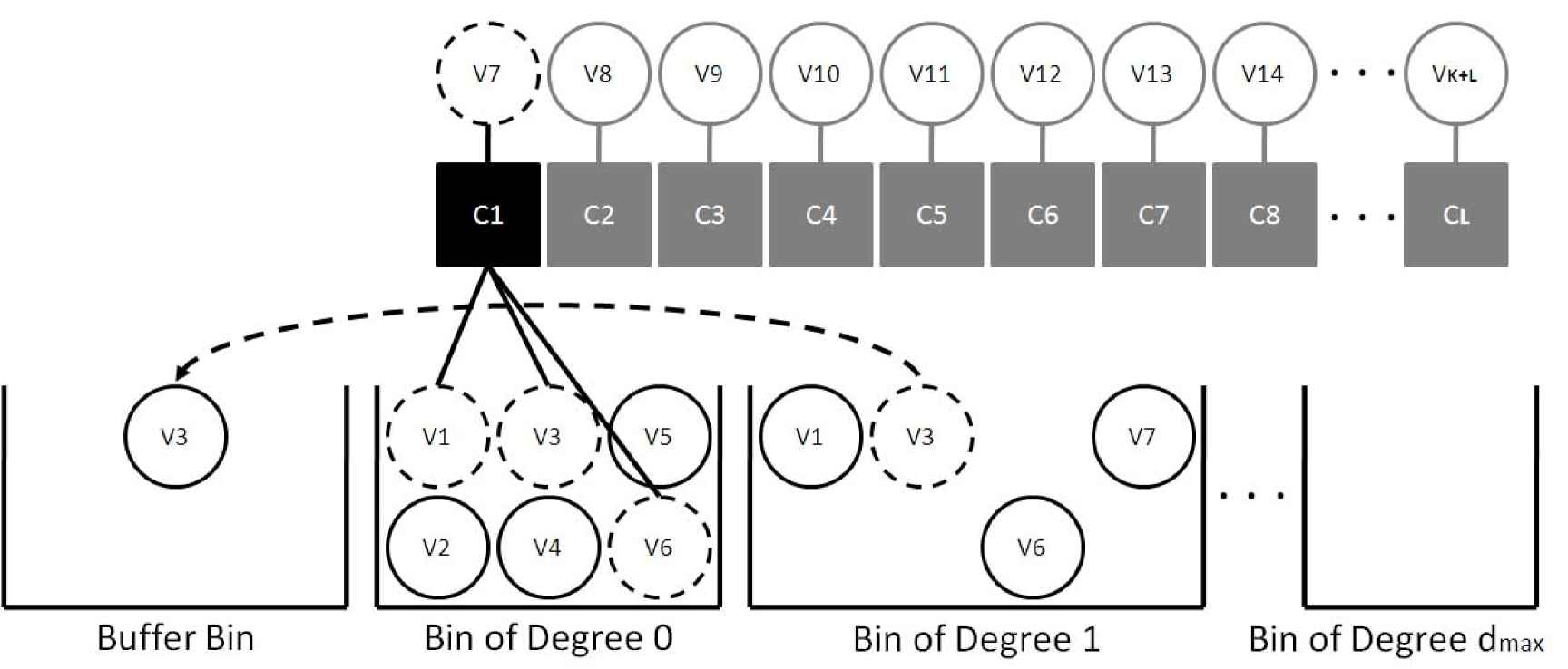
Figure 7: An instance of the ball-into-bin encoding process for $l=1$. ‘$\bigcirc$’ represents the variable balls and ‘$\blacksquare$’ the check nodes. ($K=6$)

The $1$-st encoding step ($l=1$): as shown in Fig. 7, firstly, the encoder randomly produces a degree number $i$ according to the check node degree distribution $\Omega_{i}$ and assigns it to the check node $c_{1}$. In this example, $i=4$. Since $c_{1}$ is already connected to $v_{7}$, the encoder then picks $i-1$ more variable balls out of ‘Bin of Degree $0$’ in a uniformly random manner (e.g. $v_{1}$, $v_{3}$ and $v_{6}$) and calculates the value of $v_{7}$ by combining the values of these $i-1$ balls using modulo-2 addition. From the perspective of H, the first, third, sixth and seventh columns of the first row have entries of $1$, and the other columns of the same row have entries of $0$. Secondly, the encoder moves the variable balls involved in the calculation (i.e. $v_{1}$, $v_{3}$, $v_{6}$ and $v_{7}$) to ‘Bin of Degree $1$’, since they have had one connection to the check nodes. Thirdly, the encoder randomly chooses one systematic ball $v_{j^{\prime}}$ (e.g. $v_{3}$) from those systematic ones picked in the present encoding step, and moves it into ‘Buffer Bin’. At last, the ‘Buffer Bin’ will record the degree bin from which the systematic ball comes.

The $2$-nd encoding step ($l=2$): as shown in Fig. 8, the encoder randomly produces a degree number $i$ for $c_{2}$ (e.g. $i=5$). In order to have each variable node connected to an approximately equal number of check nodes, we require the encoder to select as many variable balls as possible in the bin labeled with the lowest degree. If there are not enough balls in this bin, the encoder will take all of them and randomly choose the rest from the bin labeled with the second lowest degree. It means that balls with a lower degree have a higher priority to be chosen by the check nodes than those with a greater degree; balls sitting in the same degree bins, i.e. of the same degree, have the equal chance to be chosen. In this example, the degree number for $c_{2}$ is $i=5$, so the encoder firstly picks all the three variable balls $v_{2}$, $v_{4}$ and $v_{5}$ in ‘Bin of Degree $0$’ and randomly chooses a variable ball $v_{7}$ from ‘Bin of Degree $1$’ to calculate the value of ball $v_{8}$. Next, the encoder moves balls $v_{2}$, $v_{4}$, $v_{5}$ and $v_{8}$ to ‘Bin of Degree $1$’, and ball $v_{7}$ to ‘Bin of Degree $2$’. Finally, the encoder randomly chooses the systematic ball $v_{5}$ and moves it into ‘Buffer Bin’.

In the remaining of Phase I, a similar encoding procedure is performed for $3\leq l\leq K$. In Phase I, we require the encoder to pick at least one systematic ball in each encoding step. Each time $l$ increases by one, the encoder chooses one systematic ball, which it picks to form the encoded symbol in the $l$-th encoding step, and moves it into ‘Buffer Bin’. Systematic balls sitting in ‘Buffer Bin’ will not be picked again by the encoder to generate any other encoded symbols until Phase I ends. It means that, if a systematic ball $v_{j^{\prime}}$ is put into ‘Buffer Bin’ in the $l$-th encoding step, the ($l,j^{\prime}$)-th entry is ‘$1$’ and there will be no more entries of ‘$1$’ from the ($l+1$)-th to the $K$-th row for the $j^{\prime}$-th column. By doing so, as the encoding progresses from the $1$-st to the $K$-th step, we can obtain a matrix which is equivalent to the upper triangular sub-matrix of H in Fig. 5.

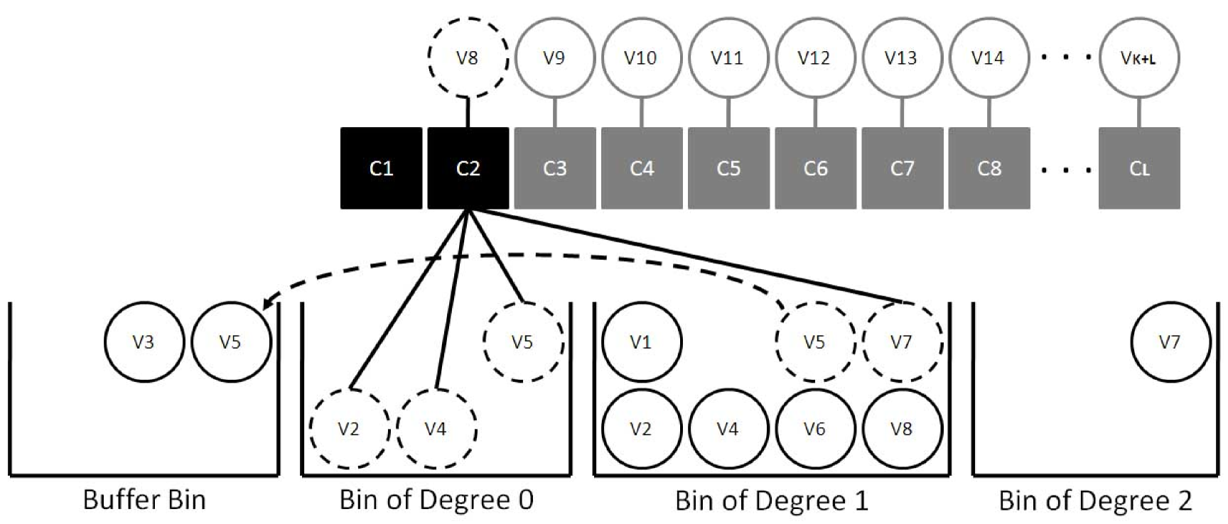
Figure 8: An instance of the ball-into-bin encoding process for $l=2$. ‘$\bigcirc$’ represents the variable balls and ‘$\blacksquare$’ the check nodes. ($K=6$)

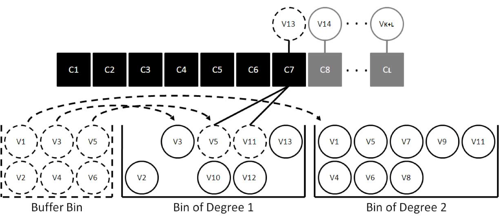
Figure 9: An instance of the ball-into-bin encoding process for $l=7$. ‘$\bigcirc$’ represents the variable balls and ‘$\blacksquare$’ the check nodes. ($K=6$)

The ($K+1$)-th encoding step ($l=K+1$): as shown in Fig. 9, Phase II of the encoding process starts. At this point, the ‘Buffer Bin’ has collected all the $K$ systematic balls. The encoder first puts all these systematic balls back into those degree bins from which they were moved to the ‘Buffer Bin’ during Phase I. Next, the encoder performs the same process as in Phase I except that the ‘Buffer Bin’ is not used, because the encoder does not move balls to ‘Buffer Bin’ in Phase II. The encoding process goes on as $l$ increases until it reaches $L$.

By following the steps above, we obtain a rateless code that can be represented by a parity-check matrix H as shown in Fig. 5. Next, we discuss the optimization of the robust check node degree distribution for a desired range of SNRs.

IV-B Optimization of the Robust Check Node Degree Distribution

The check node degree distribution is usually expressed in the polynomial form [6] and is given by

$$\Omega_{i}(x)=\sum_{i=2}^{i_{max}}\Omega_{i}x^{i}$$ (6)

So we have $\Omega_{i}(1)=1$. The check node degree distribution can be defined with respect to the nodes themselves as $\Omega_{i}(x)$ or with respect to the edges as $\omega_{i}(x)$. Let $\omega_{i}$, $i=1,2,...,i_{max}$, represent the check node degree distribution with respect to the edges, i.e. the probability that a given edge is connected to a check node of degree $i$. The degree polynomial with respect to the edges is defined by

$$\omega_{i}(x)=\sum_{i=2}^{i_{max}}\omega_{i}x^{i-1}$$ (7)

The formula for converting between the node-view and edge-view distributions is given as

$$\omega_{i}=\frac{\Omega_{i}\cdot i}{\sum_{j}\Omega\cdot j}=\frac{\Omega_{i}\cdot i}{\beta}$$ (8)

where $\beta$ is the average degree of check nodes.

Degree distributions are similarly defined for the variable nodes. We denote $\Lambda_{d}(x)=\sum_{d}\Lambda_{d}x^{d}$ and $\lambda_{d}(x)=\sum_{d}\lambda_{d}x^{d-1}$ the polynomials for the variable nodes with respect to the nodes and the edges, respectively. Assuming there are $L$ encoded symbols, and denoting by $\alpha$ the average degree of variable nodes, we have

$$\alpha(L+K)=\beta L$$ (9)

Recall that, for the proposed rateless encoding scheme with a sufficiently large $L$, the majority of variable nodes have a degree approaching the average degree $\alpha$. From (9), the variable node distribution can be approximately given by a distribution form for variable nodes in regular LDPC codes as

$$\Lambda_{d}(x)\approx x^{\alpha}=x^{\frac{\beta L}{K+L}},\quad\lambda_{d}(x)\approx x^{\frac{\beta L}{K+L}-1}$$ (10)

Alternatively, in practice, to achieve a more accurate variable node degree distribution, we can use computer simulations by first generating the variable node degree distribution many times using a fixed check node degree distribution, and then calculating the empirical mean.

The EXIT chart [20], [25] is a popular curve fitting tool widely used to optimize degree distributions. This method tracks the extrinsic mutual information between the transmitted BPSK symbols and the value of extrinsic log-likelihood ratios (L-value) in the BP decoder. Let $q$ denote the $q$-th iteration of the BP decoder. At the $q$-th iteration, an extrinsic L-value on an edge outgoing from a variable node $v$ to a check node $c$ is given by

$$LLR_{vc}^{(q)}=LLR_{ch}+\sum_{c^{\prime}\neq c}LLR_{c^{\prime}v}^{(q-1)}$$ (11)

where $LLR_{ch}$ is the L-value of the received symbols that are determined from the channel measurement. $LLR_{cv}^{(q-1)}$ is the incoming extrinsic L-value, at the $(q-1)$-th iteration, to the variable node $v$ from a check node $c$, which is in connection to this variable node, and is given by

$$LLR_{cv}^{(q-1)}=\ln\frac{1+\prod_{v^{\prime}\neq v}\tanh(\frac{LLR_{v^{\prime}c}^{(q-1)}}{2})}{1-\prod_{v^{\prime}\neq v}\tanh(\frac{LLR_{v^{\prime}c}^{(q-1)}}{2})}$$ (12)

For the initial phase where $q=0$ and from (1), we have

$$LLR_{vc}^{(0)}=LLR_{ch}=\ln\frac{p(y|x=+1)}{p(y|x=-1)}=\frac{2}{\sigma_{n}^{2}}y_{t},$$ (13)

where $p(y|x)$ is the conditional probability density function (pdf) of the signal $y$ at the output of the AWGN channel given the input signal $x\in\{\pm 1\}$. Thus, we have the variance of $LLR_{ch}$ as

$$\sigma_{ch}^{2}=\frac{4}{\sigma_{n}^{2}}$$ (14)

The EXIT chart analysis is carried out under two main assumptions. Firstly, the code Tanner graph can be represented by a tree graph [6], [26], [27], so that all involved random variables are independent. The second assumption is that the extrinsic L-values passed between nodes have a symmetric Gaussian distribution for mean $\sigma_{LLR}^{2}/2$ and variance $\sigma_{LLR}^{2}$ [20], [26]. Let function $J(\sigma_{LLR})$ denote the mutual information $I(x_{t};LLR)$ between the transmitted BPSK symbols and the extrinsic L-values with variance $\sigma_{LLR}^{2}$, which can be expressed as

$$\begin{split}&J\left(\sigma_{LLR}\right)=H(x_{t})-H(x_{t}|LLR)\\ &=1-\int_{-\infty}^{\infty}\frac{e^{-(\mu-\sigma_{LLR}^{2}/2)^{2}/2\sigma_{LLR}^{2}}}{\sqrt{2\pi\sigma_{LLR}^{2}}}\cdot\log_{2}(1+e^{-\mu})d\mu\end{split}$$ (15)

where $H(x)$ is the entropy function. Let $I_{A}$ be the average mutual information between the BPSK symbols and the L-values incoming to variable nodes, the average mutual information outgoing from variable nodes $I_{V-out}$ is then given by

$$I_{V-out}=\sum_{d=1}^{d_{max}}\lambda_{d}\cdot J\left(\sqrt{(d-1)[J^{-1}(I_{A})]^{2}+\sigma_{ch}^{2}}\right)$$ (16)

On the side of check nodes, assume that $I_{E}$ is the average mutual information between the BPSK symbols and the outgoing L-values calculated by check nodes, the average mutual information incoming to check nodes $I_{C-in}$ is given by

$$I_{C-in}=1-\sum_{i=1}^{i_{max}}\omega_{i}\cdot J\left(\frac{J^{-1}(1-I_{E})}{\sqrt{i-1}}\right)$$ (17)

The derivation of (16) and (17) is detailed in [20]. In the EXIT chart analysis, the sets of variable nodes and check nodes are respectively referred to as the variable node decoder (VND) and check node decoder (CND) [20]. These two decoders form the BP decoder. The curve $I_{V-out}\,vs.\,I_{A}$, $(0\leq I_{A}\leq 1)$, is referred to as EXIT curve of the VND, and the curve $I_{C-in}\,vs.\,I_{E}$, $(0\leq I_{E}\leq 1)$, is referred to as inverted EXIT curve of the CND. Three requirements need to be satisfied in order to achieve a near optimal degree design. Firstly, both the VND and inverted CND curves should be monotonically increasing functions and reach the $(1,1)$ point on the EXIT chart. Secondly, the VND curve should be always above the inverted CND curve. And thirdly, the VND curve has to match the shape of the inverted CND curve as accurately as possible. Consequently, the VND and inverted CND curves build an EXIT chart tunnel area. The EXIT chart analysis views iterative decoding as an evolution of the mutual information in the EXIT tunnel, starting from point $(0,I_{V-out}(0))$. When the mutual information equals one, there are no bit errors.

As the transmission progresses, i.e. the code rate changes, for a fixed degree distribution of check nodes, the inverted CND curve will stay unchanged. It is desirable if we can obtain a suitable VND curve that is unchanged as well, so that a stable EXIT chart tunnel can be obtained. From (16), it can be observed that the shape of the VND curve depends on two elements. The first element is the variable node degree distribution $\lambda_{d}$, which is in turn determined by the check node degree distribution and the number of encoded symbols. The second element for shaping the VND curve is the channel parameter $\sigma_{ch}^{2}$. This parameter $\sigma_{ch}^{2}$ determines the starting point of the VND curves, $(0,I_{V-out}(0))$, which is also the point that the evolution of the mutual information starts from in the BP decoder.

We start the design of the robust degree distribution by trying to maintain the quantity of $I_{V-out}(0)$ unchanged as the transmission goes on. Let us first consider a scenario where the SNR is sufficiently high, so that the receiver can successfully decode all the systematic message symbols as soon as it receives $K$ encoded symbols. The reason for sending encoded symbols at first, rather than sending message symbols themselves, is that the encoded symbols can provide variable nodes with protection by using parity check equations in the BP decoder. In this case, the BP decoder has $2K$ variable nodes. From Fig. 4, we can observe that these variable nodes can be divided into two sets. One set consists of the $(K+1)$-th to $2K$-th variable nodes representing $K$ encoded symbols. For this set, the variable nodes are initiated by L-values of the received symbols from the AWGN channel. From (16) and let $I_{A}=0$, the quantity of the initial average mutual information for these variable nodes is given by

$$I_{V-out}^{NZ}=J\left(\sigma_{ch}\right)$$ (18)

As shown in [20], $J\left(\sigma_{ch}\right)$ is the capacity of the channel with $\sigma_{ch}$, which in our case is the achievable code rate for the AWGN channel with BPSK modulation. For sufficiently high SNRs, $J\left(\sigma_{ch}\right)$ is close to one. The other variable node set consists of the $K$ message symbols. Since the message symbols have not been transmitted yet, the initial mutual information for these variable nodes is given by $I_{V-out}^{Z}=0$. Let $K^{\prime}$ and $\rho_{0}$ denote the number and the percentage, respectively, of the variable nodes that have zero initial mutual information in the BP decoder. We have

$$\rho_{0}=\frac{K^{\prime}}{K+L}$$ (19)

where $L$ is the number of encoded symbols. For the considered scenario, $K^{\prime}=L=K$, so $\rho_{0}=0.5$. The quantity of $I_{V-out}(0)$ is then given by

$$I_{V-out}(0)=(1-\rho_{0})\cdot I_{V-out}^{NZ}+\rho_{0}\cdot I_{V-out}^{Z}\approx 0.5$$ (20)

When SNR is lower, more symbols are necessary to be transmitted to guarantee a reliable decoding. Let us consider a scenario where SNR is about $0$dB. From Table I, we know that the achievable code rate $J\left(\sigma_{ch}\right)\approx 0.5$. From (20), we observe that it requires a near-to-zero $\rho_{0}$ to maintain $I_{V-out}(0)\approx 0.5$. A near-to-zero $\rho_{0}$ means that, either the BP decoder receives no message symbols but an infinitely large number of encoded symbols, i.e. $K^{\prime}=K$ and $L\to\infty$ in (19), or the sender starts to supply message symbols at some point of the transmission, i.e. to decrease $K^{\prime}$. The latter approach can effectively reduce $\rho_{0}$ to zero. In this paper, we refer to it as the reverse systematic transmission.

Let us represent this proposed reverse mechanism by partitioning the variable nodes into four sub-codes, namely Sub-code $A$, $B$, $C$ and $D$ as shown in the example in Fig. 4. Sub-code $C$ contains all the systematic message symbols represented by the first $K$ variable nodes. Sub-code $A$ is the first $K$ encoded symbols. The $(K+1)$-th to $\lfloor K\cdot(1+\Delta)\rfloor$-th encoded symbols constitute Sub-code $B$, where function $\lfloor x\rfloor$ represents the nearest integer to $x$, and $\Delta$ is a positive value to be determined in the optimization program. Sub-code $D$ consists of encoded symbols from the $(\lfloor K\cdot(1+\Delta)\rfloor+1)$-th encoded one to a potentially unlimited number due to the rateless property. The encoded symbols in Sub-codes $A$ and $B$ are firstly transmitted in sequence, followed by the message symbols in Sub-code $C$, and finally more encoded symbols in Sub-code $D$ are sent. The sender can transmit symbol-by-symbol. Alternatively, it can transmit block-by-block and each block consists of a fixed number of symbols. The transmission will be terminated when the sender receives an ACK response from the receiver. Next, we address the problem of optimizing the value of $\Delta$, together with the design of a robust check node degree distribution.

Similar to (20), the entire curve of $I_{V-out}\,vs.\,I_{A}$, $(0\leq I_{A}\leq 1)$, can be given by

$$\begin{split}&I_{V-out}=\\ &(1-\rho_{0})\cdot\sum_{d=1}^{d_{max}}\lambda_{d}\cdot J\left(\sqrt{(d-1)[J^{-1}(I_{A})]^{2}+\sigma_{ch}^{2}}\right)\\ &+\rho_{0}\cdot\sum_{d=1}^{d_{max}}\lambda_{d}\cdot J\left(\sqrt{d-1}J^{-1}(I_{A})\right)\end{split}$$ (21)

It shows that a tunable $\rho_{0}$ can adjust the shape of the VND curves. Thus, it is possible for us to keep the VND curve unchanged by adjusting $\rho_{0}$ while the transmission goes on. As shown in Fig. 4, for the reverse systematic transmission, the message symbols are transmitted after $\lfloor K\cdot(1+\Delta)\rfloor$ encoded symbols. When all the message symbols are received at the decoder, we have $K^{\prime}=0$, so $\rho_{0}$ would always be zero and, consequently, the decoder will lose the ability to adjust the VND curves. In order to have a tunable $\rho_{0}$, $\Delta$ is expected to be large enough so that the decoding can be successful before all the message symbols are sent. In this case, for a single SNR value of $\xi$dB, the rate of the proposed rateless code can be calculated as

$$\begin{split}R_{\xi dB}&=\frac{K}{(K+K+\Delta_{\xi dB}\cdot K)(1-\rho_{0,{\xi dB}})}\\ &=\frac{\alpha_{\xi dB}}{(1+\Delta_{\xi dB})(1-\rho_{0,{\xi dB}})}\sum_{i=2}^{i_{max}}\frac{\omega_{i}}{i}\end{split}$$ (22)

It can be observed that the actual code rate depends on the degree distributions, as well as on $\Delta_{\xi dB}$ and $\rho_{0,{\xi dB}}$. Based on this observation, an optimization program is developed to obtain a robust check node degree distribution.

Let the SNR range for the robust distribution target on $[SNR_{low},SNR_{high}]$. We choose $\tau$ SNR points within this range, where $SNR_{low}\leq SNR_{1}<SNR_{2}<...<SNR_{\tau-1}<SNR_{\tau}\leq SNR_{high}$. Let $C_{SNR_{\zeta}}$ denote the capacity of code rate corresponding to $SNR_{\zeta}$, where $1\leq\zeta\leq\tau$. Further, denote $\chi_{SNR_{\zeta}}$ as

$$\chi_{SNR_{\zeta}}=\frac{C_{SNR_{\zeta}}}{R_{SNR_{\zeta}}}$$ (23)

where $R_{SNR_{\zeta}}$ is given by (22). We want $\chi_{SNR_{\zeta}}$ to be as close to one as possible, which means $R_{SNR_{\zeta}}$ is close to the capacity. For the given $\Delta_{SNR_{\zeta}}$, $\rho_{0,SNR_{\zeta}}$ and $\alpha_{SNR_{\zeta}}$, the robust degree distribution of $\omega_{i}$ is to minimize the maximum element of

$$\{\chi_{SNR_{1}},\,\chi_{SNR_{2}},\,...,\,\chi_{SNR_{\tau-1}},\,\chi_{SNR_{\tau}}\}$$ (24)

subject to four constraints

1. $\quad\sum_{i=2}^{i_{max}}\omega_{i}=1$,

2. $\quad\omega_{i}\geq 0$,

3. $\quad|I_{V-out,SNR_{\zeta}}-I_{V-out,SNR_{\zeta^{\prime}}}|<\varepsilon,\,\textrm{where}\,\,\,\varepsilon\to 0$,

4. $\quad I_{V-out,SNR_{\zeta}}>I_{C-in}$ for $I_{A}=I_{E}$.

This optimization program can be solved by using a linear program with computer search. Condition (3) is used to enforce each pair of the VND curves being as close to each other as possible, so that a stable EXIT chart tunnel is obtained. Condition (4) is used to enforce the condition that the EXIT chart tunnel for every $SNR_{\zeta}$ point stays open. Therefore, an arbitrarily low BER can be achieved with the near-capacity transmission overhead. In addition, to reduce the transmission complexity, it is ideal to have one global $\Delta$. We propose to select that value as $\Delta=\max\{\Delta_{SNR_{1}},\Delta_{SNR_{2}},...\Delta_{SNR_{\tau-1}},\Delta_{SNR_{\tau}}\}$, covering all $\Delta_{SNR_{\zeta}}$. Generally, $\Delta$ is determined by the lowest SNR point, because the lower the SNR is, the more transmitted symbols are required. Finally, in practice, we found that it is more efficient to perform the degree optimization program by dealing with the lower SNR points first.

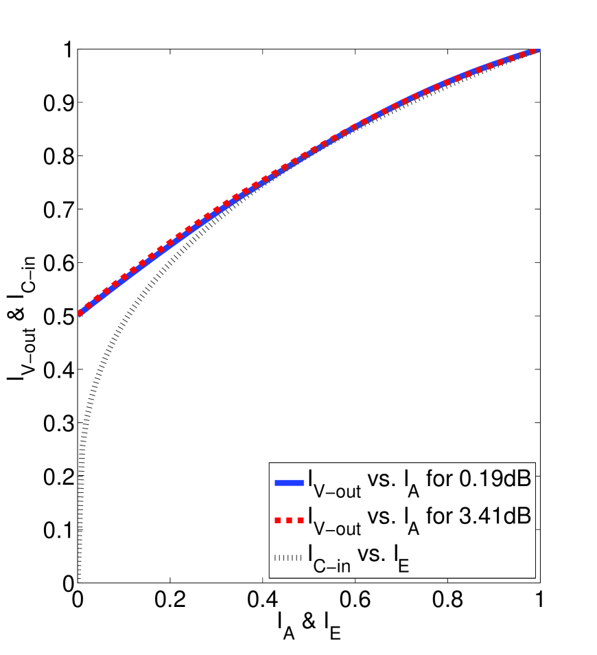
Figure 10: The EXIT chart for $I_{V-out}\,vs.\,I_{A}$ (curve of VND) and $I_{C-in}\,vs.\,I_{E}$ (inverted curve of CND)

An example of the EXIT chart resulting from the computer search for two SNR points $0.19$dB and $3.41$dB is shown in Fig. 10. These two points were chosen to correspond to a lower code rate $R_{(\sigma_{n}=0.977)}=0.501$ and a higher code rate $R_{(\sigma_{n}=0.5)}=0.912$, respectively, as shown in Table I. In this computer search, we found the values $\Delta=0.3$, $\rho_{0,\,0.19dB}=0$, $\rho_{0,\,3.41dB}=0.45$, and the robust check node degree distribution as

$$\Omega(x)=0.475x^{3}+0.525x^{6}$$ (25)

In Fig. 10, we can observe that the two respective VND curves obtained by using the robust check node degree distribution in (25) coincide with each other closely. It indicates that the system complexity can be reduced under different channel conditions.

V Simulation Results

In this section, we will present the BER performance as a function of the transmission overhead for various rateless coding schemes. BPSK modulation is used in the simulation and the transmission signal power is set to unity. We first consider two scenarios in an AWGN channel, where the noise standard deviations are $\sigma_{n}=0.977$ and $0.5$, which correspond to $0.19$ dB and $3.41$ dB, respectively, as shown in Table I. Given that the current practical code-length requirement is a few thousands [28], [29] and with regards to the necessity of sparseness in LDPC-like codes [30], the number of message symbols $K$ used in simulations is set to 2000, 3000 and 5000. The comparison is given between the proposed scheme, the non-systematic rateless code developed in [15], and the systematic rateless code in [12].

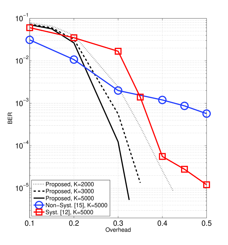
Figure 11: BER vs. Overhead for $\sigma_{n}=0.977$

Fig. 11 shows the BER performance with respect to transmission overhead $\delta$ at the low SNR region for $\sigma_{n}=0.977$. From (2) and Table I, the number of received symbols is given by

$$M=\frac{K}{0.501}(1+\delta)$$ (26)

We can observe that, for the proposed rateless code at a fixed BER level, the overhead decreases rapidly as $K$ increases. For $K=5000$, we can see that the schemes in [15] and [12] have an error floor at BER of $10^{-3}$ and $10^{-5}$ respectively, while the proposed scheme achieves significant performance improvement and the error floor has not appeared at BER of $10^{-5}$. Moreover, for BER of $10^{-5}$, the proposed scheme saves

$$M^{\prime}=\frac{5000}{0.501}\times 0.18\approx 1796$$ (27)

redundant symbols on average, i.e. almost $36\%$ of $K$, compared to the existing rateless coding schemes. The improved performance brought by the proposed rateless coding scheme is the result of the elimination of the degree-one encoded symbols and the application of the specially designed full rank parity-check matrix H. We also compared the performance of these schemes for $K=2000$ and $3000$, and obtained similar results. To simplify the illustration and reduce the number of curves, we only show the comparisons for $K=5000$ in the figure.

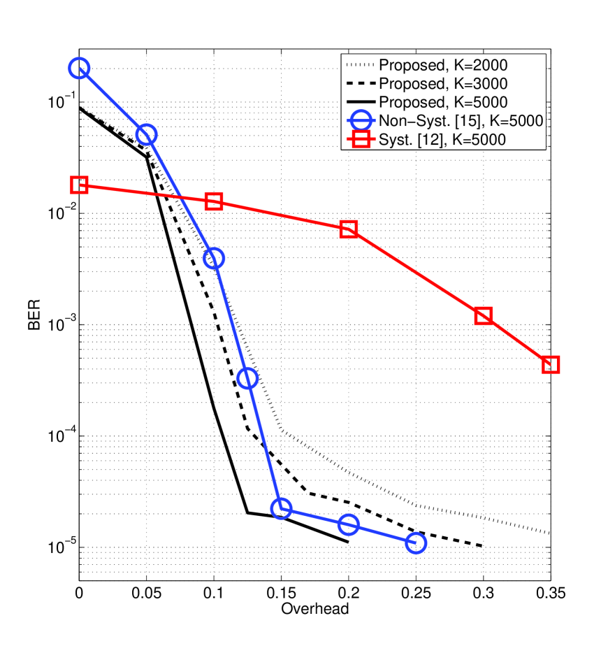
Figure 12: BER vs. Overhead for $\sigma_{n}=0.5$

Fig. 12 compares the BER performance at a higher SNR region for $\sigma_{n}=0.5$. Similarly, for the proposed code at a fixed BER level, the overhead decreases as $K$ increases. It can also be observed that the systematic code gives the worst performance for BER lower than $10^{-2}$. Although both the proposed and the non-systematic coding schemes have error floors at BER of about $10^{-5}$, the proposed scheme still outperforms the non-systematic one and saves about

$$M^{\prime}=\frac{5000}{0.912}\times 0.05\approx 274$$ (28)

redundant symbols on average, i.e. about $5.5\%$ of $K$.

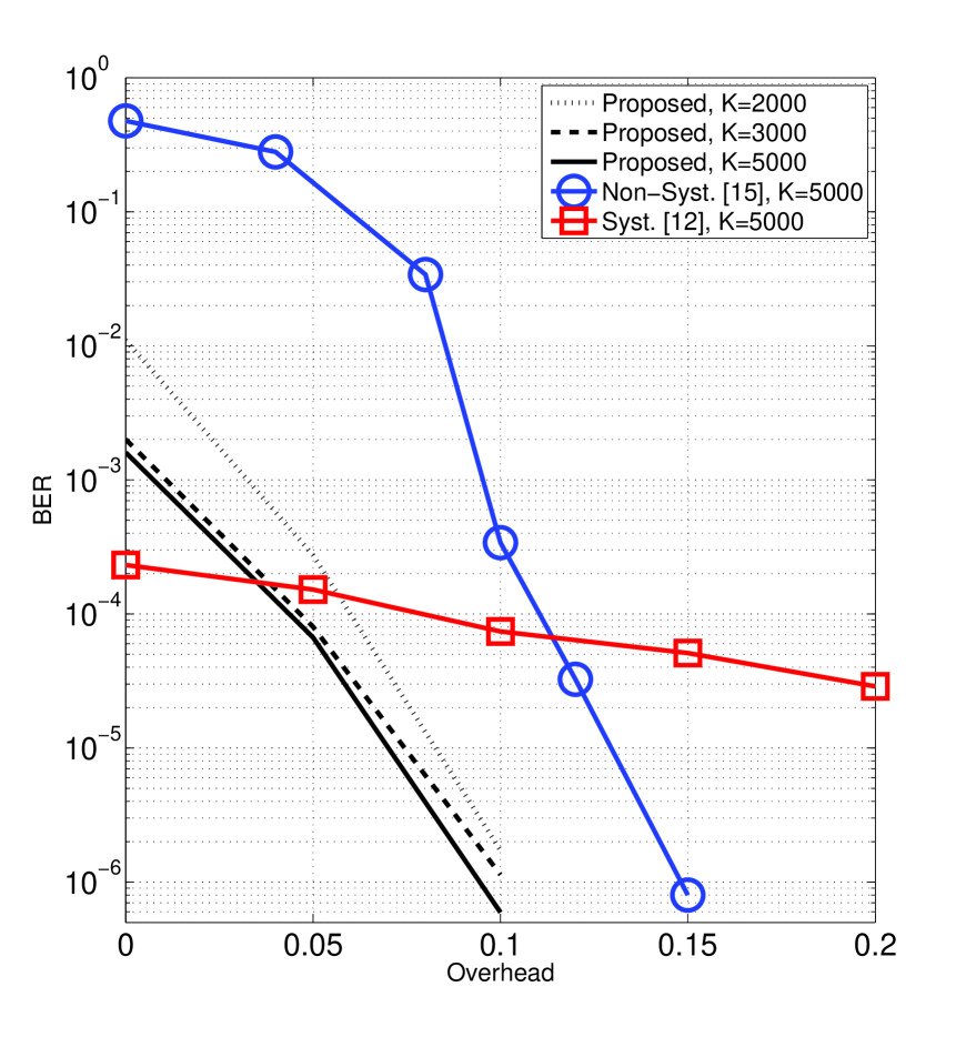
Figure 13: BER vs. Overhead for $\sigma_{n}=0.2859$

In Fig. 13, the BER performance for $\sigma_{n}=0.2859$ is plotted. We can observe that the proposed scheme has the best performance for BER better than $10^{-4}$. The same robust check node degree distribution used in Fig. 11 and Fig. 12 is also used here. For $K=2000$, BER of $10^{-5}$ is reached with overhead less than $0.1$. The results are fairly satisfactory, although the case of $\sigma_{n}=0.2859$ was not taken into consideration when we conducted the computer search in the optimization program in Section IV B.

Index	Degree Distribution $\Omega(x)$	Threshold $\sigma_{th}$
DD1	$0.475x^{3}+0.525x^{6}$	0.53
DD2	$0.1x^{2}+0.4x^{3}+0.5x^{6}$	0.525
DD3	$0.6x^{3}+0.4x^{6}$	0.44

TABLE II: Three degree distributions and their corresponding threshold values.

In addition, we provide the experimental results for different check node degree distributions to justify the use of EXIT chart analysis in the proposed encoding method. We first choose three given degree distributions, and then obtain their channel threshold parameters by using the EXIT chart approach. Thirdly, we perform simulations for the decoding performance. Results show that the degree distribution of a greater threshold does give a better decoding performance. This is consistent with the EXIT chart analysis.

We consider a code rate $R=0.8$, and the three degree distributions and their channel threshold values $\sigma_{th}$ obtained by EXIT chart analysis are given in Table II. Next, we perform simulations for the three degree distributions, which are shown as DD1, DD2 and DD3 in Fig. 14, with code-length of 6250 and 3750 symbols (i.e. the number of message symbols $K$ is 5000 and 3000 respectively). The threshold value $\sigma_{th}$ of each degree distribution is also shown in Fig. 14.

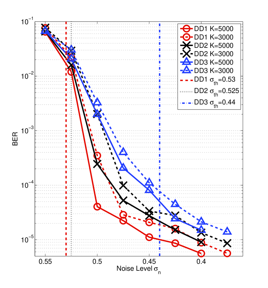
Figure 14: BER vs. Noise Level $\sigma_{n}$

From EXIT chart analysis, we know that the threshold values $\sigma_{th}$ of DD1 and DD2 are 0.53 and 0.525 respectively. Simulation results show that DD1 and DD2 have waterfall regions that closely match the threshold prediction by the EXIT chart analysis. As the code-length goes very long, we can presume an even closer match in the threshold between the simulations and the EXIT chart analysis. For DD3, it does not have clear waterfall and error floor regions, because its threshold is too far away from the Shannon limit for code rate $R=0.8$, so DD3 is far from a good distribution choice for this code rate. Overall, we come to the conclusion from simulation results that the degree distribution of a greater threshold has a better decoding performance, so the EXIT chart analysis is justified in the degree distribution design for the proposed rateless encoding method.

VI Conclusions

In this paper, we propose a physical-layer rateless coding scheme for wireless channels. A ball-into-bin method is firstly introduced to construct a particular parity-check matrix H. The aim of this method is to let both the systematic message symbols and the encoded symbols have an approximately equal degree, so that they can receive equal protection in the BP decoder. Moreover, in order to obtain a robust degree distribution of check nodes for a range of SNRs, a degree optimization program based on the EXIT chart analysis is proposed. The proposed rateless code with the robust degree distribution achieves near-capacity performances with respect to the transmission overhead. Simulation results show that the transmission redundancy is reduced as the message length increases. Moreover, under the same channel condition and transmission overhead, the BER performance of the proposed code outperforms the existing rateless codes in AWGN channels, particularly at low BER regions. For example, for BER of $10^{-5}$ and $E_{b}/N_{0}$ of $0.19$ dB, the proposed scheme saves more than one-third of the message length compared to the existing rateless schemes.

References

1. J. Byers, M. Luby, M. Mitzenmacher and A. Rege, “A digital fountain approach to reliable distribution of bulk data,” in Proc. ACM SIGCOMM, Vancouver, BC, Canada, Jan. 1998, pp. 56 - 67.

2. M. Luby, “LT codes,” in Proc. The 43rd Annual IEEE Symposium on Foundations of Computer Science, Vancouver, BC, Canada, Nov. 2002, pp. 271 - 280.

3. A. Shokrollahi, “Raptor codes,” IEEE Transactions on Information Theory, vol. 52, no. 6, pp. 2551 - 2567, June 2006.

4. R. Palanki and J. Yedidia, “Rateless codes on noisy channels,” in Proc. IEEE International Symposium on Information Theory (ISIT), Chicago, IL, June 2004, pp. 38.

5. O. Etesami, M. Molkaraie and A. Shokrollahi, “Raptor Chodes on Symmetric Channels,” in Proc. IEEE International Symposium on Information Theory (ISIT), Chicago, IL, June 2004, pp. 39.

6. O. Etesami and A. Shokrollahi, “Raptor codes on binary memoryless symmetric channels,” IEEE Transactions on Information Theory, vol. 52, no. 5, pp. 2033 - 2051, May 2006.

7. J. Castura and Y. Mao, “Raptor coding over fading channels,” IEEE Communications Letters, vol. 10, no. 1, pp. 46 - 48, Jan. 2006.

8. A. Ngo, T. Steven, G. Maunder and L. Hanzo, “A systematic LT coded arrangement for transmission over correlated shadow fading channels in 802.11 ad-hoc wireless networks,” in Proc. IEEE Vehicular Technology Conference (VTC 2010-Spring), Taipei, Taiwan, May 2010, pp. 1 - 5.

9. X. Liu and T. Lim, “Fountain codes over fading relay channels,” IEEE Transactions on Wireless Communications, vol. 8, no. 6, pp. 3278 - 3287, June 2009.

10. W. Chen and W. Chen, “A new rateless coded cooperation scheme for multiple access channels,” in Proc. IEEE International Conference on Communications (ICC), Kyoto, Japan, June 2011, pp. 1 - 5.

11. T. Jiang and X. Li, “Using fountain codes to control the peak-to-average power ratio of OFDM signals,” IEEE Transactions on Vehicular Technology, vol. 59, no. 8, pp. 3779 - 3785, Oct. 2010.

12. T. Nguyen, L. Yang and L. Hanzo, “Systematic Luby transform codes and their soft decoding,” in Proc. IEEE Workshop on Signal Processing Systems, Shanghai, China, Oct. 2007, pp. 67 - 72.

13. Z. Cheng, J. Castura and Y. Mao, “On the design of raptor codes for binary-input gaussian channels,” IEEE Transactions on Communications, vol. 57, no. 11, pp. 3269 - 3277, Nov. 2009.

14. R. Barron, C. Lo and J. Shapiro, “Global design methods for raptor codes using binary and higher-order modulations,” in Proc. IEEE Military Communications Conference, Boston, MA, Oct. 2009, pp. 1 - 7.

15. I. Hussain, M. Xiao and L. K. Rasmussen, “Error floor analysis of LT codes over the additive white Gaussian noise channel,” in Proc. IEEE Global Telecommunications Conference (GLOBECOM), Houston, USA, Dec. 2011, pp. 1 - 5.

16. R. G. Gallager, Low density parity-check codes. Cambridge, MA: MIT Press, 1963.

17. J. Garcia-Frias and W. Zhong, “Approaching Shannon performance by iterative decoding of linear codes with low-density generator matrix,” IEEE Communications Letters, vol. 7, no. 6, pp. 266 - 268, June 2003.

18. N. Bonello, R. Zhang, S. Chen and L. Hanzo, “Reconfigurable rateless codes,” IEEE Transactions on Wireless Communications, vol. 8, no. 11, pp. 5592 - 5600, Nov. 2009.

19. K. Liu and J. Garcia-Frias, “Error floor analysis in LDGM codes,” in Proc. IEEE Int. Symp. Inf. Theory (ISIT), Austin, USA, Jun. 2010, pp. 734 - 738.

20. S. ten Brink, G. Kramer and A. Ashikhmin, “Design of low-density parity-check codes for modulation and detection,” IEEE Transactions on Communications, vol. 52, no. 4, pp. 670 - 678, April 2004.

21. R. Tee, T. Nguyen, L. Yang and L. Hanzo, “Serially concatenated Luby Transform coding and bit-interleaved coded modulation using iterative decoding for the wireless internet,” in Proc. IEEE Vehicular Technology Conference, 2006-Spring, Melbourne, Australia, May 2006, pp. 22 - 26.

22. R. Tanner, “A recursive approach to low complexity codes,” IEEE Transactions on Information Theory, vol. 27, no. 5, pp. 533 - 547, Sept. 1981.

23. S. J. Johnson, Iterative error correction. Cambridge, United Kingdom: Cambridge University Press, 2010.

24. S. Lin and D. Costello, Error control coding: fundamentals and applications. Upper Saddle River, NJ, U.S.A.: Pearson Education, Inc., 2nd Edition, 2004.

25. S. ten Brink, “Convergence behavior of iteratively decoded parallel concatenated codes,” IEEE Transactions on Communications, vol. 49, no. 10, pp. 1727 - 1737, Oct. 2001.

26. T. Richardson, A. Shokrollahi and R. Urbanke, “Design of capacity approaching irregular low-density parity-check codes,” IEEE Transactions on Information Theory, vol. 47, no. 2, pp. 619 - 637, Feb. 2001.

27. M. Luby, M. Mitzenmacher and A. Shokrollahi, “Analysis of random processes via and-or tree evaluation,” in Proc. 9th Annu. ACM-SIAM Symp. Discrete Algorithms, San Francisco, CA, Jan. 1998, pp. 364 - 373.

28. IEEE standard for local and metropolitan are networks, Part 16: Air interface for fixed and mobile broadband wireless access systems. IEEE Std. 802.16, 2009.

29. IEEE 802.11n-2009: Wireless LAN Medium Access Control (MAC) and Physical Layer (PHY) Specifications: Enhancements for Higher Throughput. IEEE Std. 802.11, 2009.

30. D. MacKay, S. Wilson and M. Davey, “Comparison of construction of irregular Gallager codes,” IEEE Transactions on Communications, vol. 47, no. 10, pp. 1449 - 1454, Oct. 1999.

Shuang Tian (M’13) received the B. Sc. degree (with highest honors) from Harbin Institute of Technology, China, in 2005, the M. Eng. Sc. (Research) degree from Monash University, Australia, in 2008, and is currently working toward the Ph.D. degree at The University of Sydney, Australia, all in electrical engineering. From 2008 to 2009, he worked as a system and standard engineer with Huawei Technologies Co. Ltd., China. His research interests include coding techniques, cooperative communications, 3GPP/WiMAX network protocols, OFDM communications, and optimization of resource allocation and interference management in heterogeneous networks. He is a recipient of University of Sydney Postgraduate Awards.

Yonghui Li (M’04-SM’09) received his Ph.D. degree in November 2002 from Beijing University of Aeronautics and Astronautics. From 1999 - 2003, he was affiliated with Linkair Communication Inc, where he held a position of project manager with responsibility for the design of physical layer solutions for the LAS-CDMA system. Since 2003, he has been with the Centre of Excellence in Telecommunications, The University of Sydney, Australia. He is now an Associate Professor in School of Electrical and Information Engineering, The University of Sydney. He was the Australian Queen Elizabeth II Fellow and is currently the Australian Future Fellow. His current research interests are in the area of wireless communications, with a particular focus on MIMO, cooperative communications, coding techniques and wireless sensor networks. He holds a number of patents granted and pending in these fields. He is an executive editor for European Transactions on Telecommunications (ETT). He has also been involved in the technical committee of several international conferences, such as ICC, Globecom, etc.

Mahyar Shirvanimoghaddam received the B. Sc. degree with the 1’st Class Honour from Tehran University, Iran, in 2008, and the M. Sc. Degree with the 1’st Class Honour from Sharif University of Technology, Iran, in 2010, and is currently working toward the Ph.D. degree at The University of Sydney, Australia, all in Electrical Engineering. His research interests include coding techniques, cooperative communications, compressive sensing, and wireless sensor networks. He is a recipient of University of Sydney International Scholarship (USydIS) and University of Sydney Postgraduate Awards.

Branka Vucetic (M’83-SM’00-F’03) received the B.S.E.E., M.S.E.E., and Ph.D. degrees in 1972, 1978, and 1982, respectively, in electrical engineering, from The University of Belgrade, Belgrade, Yugoslavia. During her career, she has held various research and academic positions in Yugoslavia, Australia, and the UK. Since 1986, she has been with the Sydney University School of Electrical and Information Engineering in Sydney, Australia. She is currently the Director of the Centre of Excellence in Telecommunications at Sydney University. Her research interests include wireless communications, digital communication theory, coding, and multi-user detection. In the past decade, she has been working on a number of industry sponsored projects in wireless communications and mobile Internet. She has taught a wide range of undergraduate, postgraduate, and continuing education courses worldwide. Prof. Vucetic has co-authored four books and more than two hundred papers in telecommunications journals and conference proceedings.