The Polarization Signature of Local Bulk Flows

Abstract

A large peculiar velocity of the intergalactic medium produces a Doppler shift of the cosmic microwave background with a frequency-dependent quadrupole term. This quadrupole will act as a source for polarization of the cosmic microwave background, creating a large-scale polarization anisotropy if the bulk flow is local and coherent on large scales. In the case where we are near the center of the moving region, the polarization signal is a pure quadrupole. We show that the signal is small, but detectable with future experiments for bulk flows as large as some recent reports.

1. Introduction

The $\Lambda$CDM model of structure formation has been enormously successful in explaining a wealth of cosmological observations, including the cosmic microwave background (Bennett et al., 2013; Planck Collaboration I, 2013), galaxy clustering (Sánchez et al., 2012), and the brightness of distant supernovae (Conley et al., 2011). However, it remains an active area of research, and there have been some peculiar observations: there may be some statistically unlikely features in the cosmic microwave background (CMB) fluctuations (Bennett et al., 2011; Planck Collaboration XXIII, 2013), and there are hints that the local velocity field is not straightforward to understand in the $\Lambda$CDM framework (Watkins et al., 2009; Lavaux et al., 2010; Feldman et al., 2010; Kashlinsky et al., 2010, 2012; Colin et al., 2011; Ma et al., 2011; Magoulas et al., 2013), although many studies see good consistency (Keisler, 2009; Dai et al., 2011; Osborne et al., 2011; Nusser & Davis, 2011; Turnbull et al., 2012; Mody & Hajian, 2012; Branchini et al., 2012; Ma & Scott, 2013; Rathaus et al., 2013).

Independent probes of such anomalies would be invaluable. For example, Zhang & Stebbins (2011) used small-scale temperature anisotropies in the CMB as a probe of large-scale inhomogeneities in the universe.

In this work we demonstrate that large angle CMB polarization can be similarly used to measure large-scale bulk flows. In §2 we show this polarization signal, along with its unique frequency dependence, §3 estimates the expected magnitude of the effect, §4 uses data from the Wilkinson Microwave Anisotropy Probe (WMAP) to put limits on this signal, while §5 forecasts future constraints possible on large-scale bulk flows.

2. CMB Anisotropy from a Local Bulk Flow

CMB anisotropy caused by our peculiar velocity is a well-understood phenomenon, as the dipole has long been used as a measurement of the bulk velocity of the Earth (e.g. Smoot et al., 1977) and the annual modulation of the dipole due to the Earth’s orbit is now used as a CMB calibration source (Bennett et al., 2013; Planck Collaboration VI, 2013). Planck Collaboration XXVII (2013) has also measured the effect on the small-scale CMB anisotropies due to the Doppler ‘modulation’ and ‘aberration’ resulting from our motion relative to the CMB.

In a related effect, electrons with peculiar velocities act as a source for CMB polarization (Baumann et al., 2003). An electron moving with peculiar velocity $\beta\equiv v/c$ sees a boosted CMB spectrum:

$$I_{\nu}=Cx^{3}\left[\exp\left(x\frac{1+\beta\mu}{\sqrt{1-\beta^{2}}}\right)-1\right]^{-1}$$ (1)

where $C=2(k_{B}T_{\text{CMB}})^{3}/(hc)^{2}$, $x=h\nu/k_{B}T_{\text{CMB}}$ and $\mu$ is the cosine of the angle between the incoming photon direction and the direction of the velocity. Expanding in terms of $\beta$ we see that

$$I_{\nu}= \frac{Cx^{3}}{e^{x}-1}\left\{1-\frac{xe^{x}}{e^{x}-1}\mu\beta\right.$$

$$\left.{}+\frac{xe^{x}}{e^{x}-1}\left[\left(\frac{x}{2}\coth\frac{x}{2}\right)\mu^{2}+\frac{1}{2}\right]\beta^{2}+\mathcal{O}(\beta^{3})\right\}.$$ (2)

The first order term in $\beta$ is the well-studied CMB dipole, with the frequency dependence of a pure fluctuation in temperature: $(Cx^{3}/e^{x}-1)(xe^{x}/e^{x}-1)$. At second order, there is a component that again corresponds to a pure temperature fluctuation, but also a term with a non-thermal spectrum, which has been discussed extensively in Kamionkowski & Knox (2003).

This non-thermal second-order term can be decomposed into quadrupole ($\propto\mu^{2}-1/3$) and monopole terms, so that if we divide out the thermal frequency dependence and expand it in spherical harmonics, it becomes

$$\left(\frac{x}{2}\coth\frac{x}{2}\right)\mu^{2}=2\sqrt{\frac{4\pi}{5}}\left(\frac{x}{2}\coth\frac{x}{2}\right)\left(\frac{1}{3}Y_{20}+\sqrt{4\pi}Y_{00}\right).$$ (3)

The coordinate system has been set by aligning the z-axis with the direction of motion. In temperature units, the ‘kinematic’ quadrupole seen by the electron and resulting from its motion is therefore

$$a^{e^{-}}_{20}=\frac{2}{3}\sqrt{\frac{4\pi}{5}}g(x)T_{\text{CMB}}\beta^{2},$$ (4)

where the non-thermal frequency dependence is given by $g(x)=x/2\,\coth(x/2)$ (see Fig. 1).

Figure 1.— The non-thermal frequency dependence of the quadrupole anisotropy induced by a peculiar velocity.

More generally, if the velocity points in the direction $\mathbf{\hat{v}}=(\theta_{v},\phi_{v})$ and the incoming photon direction is $\mathbf{\hat{n}}$, the quadrupole term in (2) becomes

$$\mu^{2}-\frac{1}{3} =\frac{2}{3}P_{2}(\mathbf{\hat{v}}\cdot\mathbf{\hat{n}})$$ (5)

$$=\frac{8\pi}{15}\sum_{m=-2}^{2}Y_{2m}^{*}(\theta_{v},\phi_{v})Y_{2m}(\mathbf{\hat{n}})$$ (6)

where $P_{2}$ is the second order Legendre polynomial. Therefore, the kinematic quadrupole moments of the local radiation field can be expressed as

$$a^{e^{-}}_{2m}=\frac{8\pi}{15}g(x)T_{\text{CMB}}\beta^{2}Y^{*}_{2m}(\theta_{v},\phi_{v}).$$ (7)

Thomson scattering of such a quadrupole anisotropy in the light seen by the electron will create linear polarization in the scattered radiation. In particular, the $a^{e^{-}}_{2\pm 2}$ quadrupole will generate polarization along the outgoing $z$-axis (Kosowsky, 1999). The Stokes $Q$ and $U$ parameters of the scattered radiation along the $\hat{z}$ axis are

$$Q(\hat{z})\pm iU(\hat{z})=\sigma_{T}\sqrt{\frac{3}{40\pi}}a^{e^{-}}_{2,\mp 2}\ .$$ (8)

We will use this result to calculate the polarization emitted in all directions. Following Kosowsky (1999), we rotate the the incoming field through the Euler angles $(\theta_{e},\phi_{e})$ so that the multipole coefficients in this rotated basis are

$$\tilde{a}_{\ell m}^{e^{-}}=\!\!\!\sum_{m^{\prime}=-m}^{m}\!\!\!\mathcal{D}_{m^{\prime}m}^{\ell\,*}(\theta_{e},\phi_{e},0)a^{e^{-}}_{\ell m^{\prime}}$$ (9)

where $\mathcal{D}_{m^{\prime}m}^{\ell}$ is the Wigner rotation symbol. The polarization emitted in the direction $(\theta_{e},\phi_{e})$ will be generated by $\tilde{a}^{e^{-}}_{2,\pm 2}$:

$$\tilde{a}^{e^{-}}_{2,\pm 2}=\sum_{m}\mathcal{D}_{m,\pm 2}^{2\,*}(\theta_{e},\phi_{e},0)\,a_{2m}^{e^{-}}.$$ (10)

The Wigner rotation can be expressed in terms of spin-weighted spherical harmonics (Goldberg et al., 1967; Hu & White, 1997):

$$\tilde{a}^{e^{-}}_{2,\pm 2}=\sqrt{\frac{4\pi}{5}}\sum_{m}{{}_{\mp 2}}Y_{2m}^{*}(\theta_{e},\phi_{e})\,a_{2m}^{e^{-}}.$$ (11)

Therefore, the polarization emitted in the direction $(\theta_{e},\phi_{e})$ from scattering by a single electron moving in the direction $(\theta_{v},\phi_{v})$ is

$$Q(\theta_{e},\phi_{e})\pm iU(\theta_{e},\phi_{e})=\sigma_{T}\sqrt{\frac{3}{50}}\sum_{m}\!{{}_{\pm 2}}Y_{2m}^{*}(\theta_{e},\phi_{e})\,a_{2m}^{e^{-}}.$$ (12)

To express this in terms of the polarization measured in direction $(\theta,\phi)$ by an observer (see Fig. 2), note that $\theta_{e}=\pi-\theta$ and $\phi_{e}=\phi+\pi$. We find that

$${{}_{\pm 2}}Y^{*}_{2m}(\theta_{e},\phi_{e})=(-1)^{|m|}{{}_{\pm 2}}Y_{2,-m}(\theta,\phi),$$ (13)

and so the polarization observed in the direction $(\theta,\phi)$ is

$$Q(\theta,\phi)\pm iU(\theta,\phi)=\sigma_{T}\sqrt{\frac{3}{50}}\sum_{m}(-1)^{|m|}{{}_{\pm 2}}Y_{2m}(\theta,\phi)\,a_{2,-m}^{e^{-}}.$$ (14)

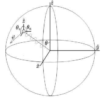
Figure 2.— The geometry of a single polarized Thomson scattering as seen by an observer at the origin.

Any parcel of electrons that is moving relative to the CMB will therefore generate polarization anisotropy. If a large local volume has a substantial bulk flow there could be a large scale polarization signal. The total polarization can be calculated by substituting (7) into (14) and integrating the contribution for all electrons along the line of sight:

$$Q(\theta,\phi)\pm\, iU(\theta,\phi)=g(x)T_{\text{CMB}}\sqrt{\frac{3}{50}}\frac{8\pi}{15}$$

$$\times\int dr\Big{(}a(r)\sigma_{T}n_{e}(\theta,\phi,r)\beta^{2}(\theta,\phi,r)$$

$$\times\sum_{m}Y_{2m}[\theta_{v}(r,\theta,\phi),\phi_{v}(r,\theta,\phi)]\,{{}_{\pm 2}}Y_{2m}(\theta,\phi)\Big{)}.$$ (15)

For a general density and velocity distribution, equation (15) leads to a complicated polarization pattern, as there could be spatial (radial and angular) variation of $n_{e}$, $\beta$, $\theta_{v}$, and $\phi_{v}$.

In cases where there is some symmetry, it can be helpful to re-express (15) in terms of the E and B modes defined by sums and differences of the spin-2 spherical harmonics (Zaldarriaga & Seljak, 1997). If there is no angular dependence to the electron densities and velocities, the expansion coefficients for the spin-2 spherical harmonics can be simply read off the above equation as the coefficients of ${{}_{\pm 2}}Y_{2m}(\theta,\phi)$.

In a model where the observer is located at the center of a spherical region of a bulk flow with constant direction but radially varying amplitude and constant electron density, the signal will be a pure E-mode quadrupole:

$$a^{E}_{2m} \equiv-\frac{1}{2}({{}_{2}}a_{2m}+{{}_{-2}}a_{2m})$$ (16)

$$=-g(x)T_{\text{CMB}}\frac{8\pi}{15}\sqrt{\frac{3}{50}}$$

$$\qquad\times\int dr\,a(r)\sigma_{T}n_{e}\beta^{2}(r)Y_{2m}(\theta_{v}(r),\phi_{v}(r))$$ (17)

and

$$a^{B}_{2m} \equiv-\frac{i}{2}({{}_{2}}a_{2m}-{{}_{-2}}a_{2m})=0$$ (18)

In the even simpler case where we assume a sphere of constant velocity out to a redshift $z_{r}$, the integral $\int dr\,\sigma_{T}n_{e}a(r)$ is equivalent to the optical depth to $z_{r}$, $\tau(z_{r})$, and (17) becomes

$$a^{E}_{2m}=-g(x)T_{\text{CMB}}\tau(z_{r})\beta^{2}\frac{8\pi}{15}\sqrt{\frac{3}{50}}Y_{2m}(\theta_{v},\phi_{v}).$$ (19)

In a coordinate system where the z-axis is aligned with the bulk flow direction, the entire signal is contained in a single quadrupole moment with magnitude

$$a^{E}_{20}=-\frac{2}{5}\sqrt{\frac{2\pi}{15}}g(x)T_{\text{CMB}}\tau(z_{r})\beta^{2}.$$ (20)

Since the velocity of the bulk flow, $\beta^{2}$, and its extent, $\tau(z_{r})$, are degenerate, we will reparameterize equation (19), using

$$A_{\text{flow}}=\tau(z_{r})\beta^{2},$$ (21)

so that

$$a^{E}_{2m}=-A_{\text{flow}}g(x)T_{\text{CMB}}{\frac{8\pi}{15}}\sqrt{\frac{3}{50}}Y_{2m}(\theta_{v},\phi_{v}).$$ (22)

3. Polarization signatures of recent bulk flow measurements

In recent years, there have been many surveys of local peculiar velocities. Some of these surveys have reported consistency with the predictions of $\Lambda$CDM (e.g. Nusser & Davis, 2011; Turnbull et al., 2012; Dai et al., 2011; Keisler, 2009; Osborne et al., 2011) However, there have also been several reports of anomalously large values (e.g. Watkins et al., 2009; Lavaux et al., 2010; Feldman et al., 2010; Colin et al., 2011; Kashlinsky et al., 2010, 2012).

One such measurement of a bulk flow somewhat larger than that predicted by linear-theory $\Lambda$CDM is due to Feldman et al. (2010), who compiled the results of most prior major peculiar velocity surveys. They measure a bulk flow of $416\pm 78$ km/s using a $100h^{-1}$Mpc Gaussian window, which they find to be in tension with $\Lambda$CDM.

A second case is given by the measurements of Kashlinsky et al. (2010) using the kSZ signal produced by hot gas in galaxy clusters. They report a bulk flow of 1000 km/s on scales of $\gtrsim 550h^{-1}$Mpc, although the significance of this measurement has been contested (Keisler, 2009; Osborne et al., 2011; Mody & Hajian, 2012; Lavaux et al., 2013; Planck Collaboration Int. XIII, 2013). This measurement is inconsistent with $\Lambda$CDM. Additionally, the authors propose that the bulk flow measured could be a piece of a ‘dark flow’ extending out to the horizon, as would be expected for a ‘tilted universe’ (Turner, 1991; Ma et al., 2011).

Since the reported bulk flows span a wide range of sizes, we investigate several scenarios to determine the possible resulting polarization signals. Our four scenarios are summarized in Table 1, and represent:

• a ‘small’ bulk flow consistent with $\Lambda$CDM predictions

• a ‘medium’ bulk flow in tension with $\Lambda$CDM, approximating the results of Feldman et al. (2010)

• a ‘large’ bulk flow inconsistent with $\Lambda$CDM, approximating the results of Kashlinsky et al. (2010)

• a large ‘dark flow’ similar to that proposed by Kashlinsky et al. (2010), extending to at least the redshift of reionization (but not to recombination)

	Velocity (km/s)	$z_{r}$	$-a_{20}^{E}$ (nK)	$A_{\text{flow}}$
Small	100	0.03	0.006	$6\times 10^{-12}$
Medium	400	0.03	0.1	$9\times 10^{-11}$
Large	1000	0.25	6	$6\times 10^{-9}$
Dark Flow	1000	$\gtrsim 10.6$	1000	$1\times 10^{-6}$

Table 1Polarization signal for local bulk flows at $\nu=150$ GHz

For comparison, the cosmological E-modes on these scales are of order 100 nK on horizon scales, while B-modes from inflation on the largest scales would have an amplitude of order 1 nK for a tensor-to-scalar ratio of order $r\sim 10^{-4}$. While it is a small signal, the characteristic frequency dependence $g(x)$ of the contribution from bulk flows makes such a measurement at least possible in principle.

In comparison to the secondary anisotropies induced by the thermal Sunyaev-Zel’dovich effect (tSZ), with a nominal expected $y\sim 10^{-6}$, the bulk flow signal, which varies as $\tau\beta^{2}$, is smaller (see the $A_{\text{flow}}$ column in Table 1). Indeed, its frequency dependence is a linear combination of the frequency dependences of thermal fluctuations and tSZ. However, it is a large-scale polarization signal, whereas $y$ fluctuations occur on small scales and are unpolarized to leading order. We will discuss the possibility of confusion from the polarized tSZ in §4.

4. Constraints on bulk flows from large-angle CMB polarization data

A very large bulk velocity extending across a significant portion of the universe could be detectable by WMAP. We will therefore use WMAP9 polarization data (Bennett et al., 2013) to put an upper limit on the bulk flow. We perform a $\chi^{2}$ fit of the WMAP data for $A_{\text{flow}}$, using the foreground-reduced V-band maps. We extract the quadrupoles from the WMAP maps and compare them to equation (22) with freely varying $A_{\text{flow}}$ but velocity fixed in the direction found by Kashlinsky et al. (2010): $(l,b)=(288^{\circ},30^{\circ})$. We choose this direction in the hope of constraining their proposed ‘dark flow’ since all other claimed signals would be too small to be measured by WMAP.

The variance in the $\chi^{2}$ fit is given by

$$C_{2}=C_{2}^{\text{theory}}+N_{2},$$ (23)

where $C_{2}^{\text{theory}}$ is the theoretical value of the EE power spectrum at $\ell=2$ and $N_{2}$ is the experimental noise of the E mode quadrupole, which we estimated by averaging the nearby WMAP BB $C_{\ell}$’s in the same map. Since WMAP does not detect a physical B mode signal, the measured BB power spectrum is an estimate of the E mode noise on the same scales.

Figure 3.— The results of the $\chi^{2}$ fit for $A_{\text{flow}}$ along the direction found by Kashlinsky et al. (2010).

Since the bulk flow signal is frequency-dependent, the foreground removal process may decrease the signal present in these maps. However, $g(x)$ does not vary greatly over the WMAP bands, so we expect this to be a small effect. Constraints on the bulk flow amplitude are shown in Figure 3. We find a 95% upper limit of $A_{\text{flow}}=3\times 10^{-6}$, which corresponds to a bulk flow of order 2000 km/s extending out to reionization. Stronger constraints will require lower noise, as well as multi-frequency combinations (to suppress primary CMB fluctuations).

With ongoing rapid improvements in polarization sensitivity, we can expect big improvements in these sorts of measurements. At $\ell=2$, the expected polarization sensitivity of the Planck experiment is of order 15 nK, only slightly greater than the signal expected for the large flow observed by Kashlinsky et al. (2010). Future CMB satellites such as PIXIE (Kogut et al., 2011) or EPIC (Bock et al., 2008) could have sensitivity better than 2 nK, which would be sufficient to detect this signal. Moreover, an experiment like PIXIE, which would make measurements in many frequency bands over a very wide range, would be ideal for separating the bulk flow signal from the primary CMB anisotropies.

No experiments currently planned would be capable of measuring the signal predicted by $\Lambda$CDM, which are at least an order of magnitude lower in amplitude. In general, the signal expected from $\Lambda$CDM will look quite different from our model, since we have only included the the contribution of a local bubble. It is also small enough that there will be a term of comparable size from the polarized tSZ. This signal results from the isotropic thermal motion of electrons, coupled to anisotropy in the CMB. Since the frequency dependence of the bulk flow signal is a linear combination of the frequency dependence for a thermal fluctuation and a tSZ fluctuation, the polarized tSZ will ultimately place a limit on how precisely the bulk flow can be measured.

We can estimate the magnitudes of the two signals by considering that the bulk flow signal varies as $\tau\beta_{\text{BF}}^{2}T_{0}$ (where $T_{0}$ is the CMB monopole), while the polarized tSZ goes as $\tau\sigma_{e}^{2}T_{2}$ (where $T_{2}$ is the CMB quadrupole and $\sigma_{e}^{2}$ is the rms velocity of the electrons). The terms $\sigma_{e}^{2}$ and $\beta_{\text{BF}}^{2}$ are both set by the local gravitational potentials, but the thermal energy of the electrons is enhanced by a factor of $m_{p}/m_{e}\sim 2000$. Since $T_{2}\sim 10^{-5}T_{0}$, we estimate the polarized tSZ to be smaller than the bulk flow signal by a factor of $\sim 10^{-2}$. In general, we expect that for a $\Lambda$CDM bulk flow, the polarized tSZ signal will generally be smaller but non-negligible for precise measurements.

The quadrupolar polarized foregrounds are of order 1 $\mu$K, so considerable foreground reduction will be required. Additionally, since the frequency dependence of this signal is equivalent to a linear combination of the primary CMB and tSZ signals, leakage of tSZ temperature signal into the polarization will form a significant source of error for attempted detections. For many experiments, an important source of temperature-polarization leakage results from a slightly elliptic beam, which, when rotated, leads to a spurious coupling of the polarization with the local unpolarized quadrupole.

We expect that future CMB polarization experiments designed to detect primordial B modes may be able to measure the polarization produced by bulk flows. For these experiments, the beam ellipticity should be of order $0.01$% (Bock et al., 2006). Extrapolating from the Planck tSZ power spectrum (Planck Collaboration XXI, 2013), we estimate a quadrupole term of $\sim 0.03$ $\mu$K, implying a spurious polarization signal due to tSZ with amplitude $\sim 0.003$ nK. This is close in size to our ‘small’ model, and represents another potential difficulty for detection. However, future experiments will be able to effectively constrain anomalous large scale bulk flows.

5. Discussion

We have presented a new probe of large scale bulk flows in the universe. In general, the induced polarization anisotropy will have a well-defined frequency dependence but would have complicated angular structure. In the simple case of large local bulk flows, WMAP data is able to rule out flows that are only slightly larger than the largest ones proposed. Planck will have the sensitivity to rule out horizon-scale bulk flows and put strong limits on the proposed “dark flow” of Kashlinsky et al. (2010).

With a unique frequency dependence, these observations should be separable from both primary CMB fluctuations and from foregrounds. While the $\ell=2$ mode (quadrupole) is the simplest to understand as a simple large-scale local bulk flow, there will be interesting signatures on a variety of angular scales. While such bulk flows can also be mapped using the kinetic Sunyaev-Zel’dovich effect, the polarization signature offers a complementary view of the large scale motions of cosmic gas. The kinetic polarization signal is most sensitive to velocities perpendicular to the line of sight, whereas the kinetic Sunyaev-Zel’dovich effect is sensitive to velocities projected along the line of sight, suggesting that measurements of the two effects can be combined to measure the three-dimensional velocity field.

Such large scale bulk flows are unlikely to exist in the framework of the $\Lambda$CDM model of structure formation, and represent one of a number of possible anomalous deviations from $\Lambda$CDM. In spite of the many measurements of our local velocity field, it is not yet clear whether the local peculiar velocities are consistent with expectations. In particular, although the CMB dipole is believed to arise from a Doppler shift due to our velocity with respect to the CMB, measurements of local peculiar velocities have not been able to completely account for it (Kocevski & Ebeling, 2006).

As a result, it is of interest to have multiple independent probes of the large-scale velocity field. Since the bulk flow polarization signal described here is most sensitive to large-scale flows, unlike most standard peculiar velocity measurements, it may have the potential to provide a consistency test for better understanding the CMB dipole and the local velocity field on large scales.

We thank Olivier Doré for valuable discussions. This work was supported by NSERC, CIfAR, and the Canada Research Chairs program. This work was supported in part by the National Science Foundation under Grant No. PHYS-1066293 and the hospitality of the Aspen Center for Physics. Some of the results in this paper have been derived using the HEALPix (Górski et al., 2005) package. We acknowledge the use of the Legacy Archive for Microwave Background Data Analysis (LAMBDA), part of the High Energy Astrophysics Science Archive Center (HEASARC). HEASARC/LAMBDA is a service of the Astrophysics Science Division at the NASA Goddard Space Flight Center.

References

- Baumann et al. (2003) Baumann, D., Cooray, A., & Kamionkowski, M. 2003, New Astron., 8, 565
- Bennett et al. (2011) Bennett, C. L., Hill, R. S., Hinshaw, G., et al. 2011, ApJS, 192, 17
- Bennett et al. (2013) Bennett, C. L., Larson, D., Weiland, J. L., et al. 2013, ApJS, 208, 20
- Bock et al. (2006) Bock, J., Church, S., Devlin, M., et al. 2006, arXiv:astro-ph/0604101
- Bock et al. (2008) Bock, J., Cooray, A., Hanany, S., et al. 2008, arXiv:0805.4207
- Branchini et al. (2012) Branchini, E., Davis, M., & Nusser, A. 2012, MNRAS, 424, 472
- Colin et al. (2011) Colin, J., Mohayaee, R., Sarkar, S., & Shafieloo, A. 2011, MNRAS, 414, 264
- Conley et al. (2011) Conley, A., Guy, J., Sullivan, M., et al. 2011, ApJS, 192, 1
- Dai et al. (2011) Dai, D.-C., Kinney, W. H., & Stojkovic, D. 2011, JCAP, 4, 15
- Feldman et al. (2010) Feldman, H. A., Watkins, R., & Hudson, M. J. 2010, MNRAS, 407, 2328
- Goldberg et al. (1967) Goldberg, J. N., Macfarlane, A. J., Newman, E. T., Rohrlich, F., & Sudarshan, E. C. G. 1967, J. Math. Phys., 8, 2155
- Górski et al. (2005) Górski, K. M., Hivon, E., Banday, A. J., et al. 2005, ApJ, 622, 759
- Hu & White (1997) Hu, W., & White, M. 1997, Phys. Rev. D, 56, 596
- Kamionkowski & Knox (2003) Kamionkowski, M., & Knox, L. 2003, Phys. Rev. D, 67, 063001
- Kashlinsky et al. (2012) Kashlinsky, A., Atrio-Barandela, F., & Ebeling, H. 2012, arXiv:1202.0717
- Kashlinsky et al. (2010) Kashlinsky, A., Atrio-Barandela, F., Ebeling, H., Edge, A., & Kocevski, D. 2010, ApJ, 712, L81
- Keisler (2009) Keisler, R. 2009, ApJ, 707, L42
- Kocevski & Ebeling (2006) Kocevski, D. D., & Ebeling, H. 2006, ApJ, 645, 1043
- Kogut et al. (2011) Kogut, A., Fixsen, D. J., Chuss, D. T., et al. 2011, JCAP, 7, 25
- Kosowsky (1999) Kosowsky, A. 1999, New Astron. Rev., 43, 157
- Lavaux et al. (2013) Lavaux, G., Afshordi, N., & Hudson, M. J. 2013, MNRAS, 430, 1617
- Lavaux et al. (2010) Lavaux, G., Tully, R. B., Mohayaee, R., & Colombi, S. 2010, ApJ, 709, 483
- Ma et al. (2011) Ma, Y.-Z., Gordon, C., & Feldman, H. A. 2011, Phys. Rev. D, 83, 103002
- Ma & Scott (2013) Ma, Y.-Z., & Scott, D. 2013, MNRAS, 428, 2017
- Magoulas et al. (2013) Magoulas, C., Springob, C., Colless, M., et al. 2013, in IAU Symposium, Vol. 289, IAU Symposium, ed. R. de Grijs, 402–405
- Mody & Hajian (2012) Mody, K., & Hajian, A. 2012, ApJ, 758, 4
- Nusser & Davis (2011) Nusser, A., & Davis, M. 2011, ApJ, 736, 93
- Osborne et al. (2011) Osborne, S. J., Mak, D. S. Y., Church, S. E., & Pierpaoli, E. 2011, ApJ, 737, 98
- Planck Collaboration I (2013) Planck Collaboration I. 2013, A&A, submitted (arXiv:1303.5062)
- Planck Collaboration Int. XIII (2013) Planck Collaboration Int. XIII. 2013, A&A, submitted (arXiv:1303.5090)
- Planck Collaboration VI (2013) Planck Collaboration VI. 2013, A&A, submitted (arXiv:1303.5067)
- Planck Collaboration XXI (2013) Planck Collaboration XXI. 2013, A&A, submitted (arXiv:1303.5081
- Planck Collaboration XXIII (2013) Planck Collaboration XXIII. 2013, A&A, submitted (arXiv:1303.5083)
- Planck Collaboration XXVII (2013) Planck Collaboration XXVII. 2013, A&A, submitted (arXiv:1303.5087)
- Rathaus et al. (2013) Rathaus, B., Kovetz, E. D., & Itzhaki, N. 2013, MNRAS, 431, 3678
- Sánchez et al. (2012) Sánchez, A. G., Scóccola, C. G., Ross, A. J., et al. 2012, MNRAS, 425, 415
- Smoot et al. (1977) Smoot, G. F., Gorenstein, M. V., & Muller, R. A. 1977, Phys. Rev. Lett., 39, 898
- Turnbull et al. (2012) Turnbull, S. J., Hudson, M. J., Feldman, H. A., et al. 2012, MNRAS, 420, 447
- Turner (1991) Turner, M. S. 1991, Phys. Rev. D, 44, 3737
- Watkins et al. (2009) Watkins, R., Feldman, H. A., & Hudson, M. J. 2009, MNRAS, 392, 743
- Zaldarriaga & Seljak (1997) Zaldarriaga, M., & Seljak, U. 1997, Phys. Rev. D, 55, 1830
- Zhang & Stebbins (2011) Zhang, P., & Stebbins, A. 2011, Phys. Rev. Lett., 107, 041301