A determination of the space density and birth rate of hydrogen-line (DA) white dwarfs in the Galactic Plane, based on the UVEX survey

Abstract

We present a determination of the average space density and birth rate of hydrogen-line (DA) white dwarfs within a radius of 1 kpc around the Sun, based on an observational sample of 360 candidate white dwarfs with $g$$<$19.5 and $(g-r)$$<$0.4, selected from the UV-excess Survey of the Northern Galactic Plane (UVEX ), in combination with a theoretical white dwarf population that has been constructed to simulate the observations, including the effects of reddening and observational selection effects. The main uncertainty in the derivation of the white dwarf space density and current birth rate lies in the absolute photometric calibration and the photometric scatter of the observational data, which influences the classification method on colours, the completeness and the pollution. Corrections for these effects are applied. We derive an average space density of hydrogen-line (DA) white dwarfs with $T_{\rm eff}$$>$10 000K ($M_{V}$$<$12.2) of (3.8 $\pm$ 1.1) $\times$ 10^-4 pc^-3, and an average DA white dwarf birth rate over the last 7$\times$10⁷ years of (5.4 $\pm$ 1.5) $\times$ 10^-13 pc^-3yr^-1. Additionally, we show that many estimates of the white dwarf space density from different studies are consistent with each other, and with our determination here.

1 Introduction

One of the main goals of the European Galactic Plane Surveys (EGAPS ) is to obtain a homogeneous sample of stellar remnants in our Milky Way with well-understood selection limits. The population of white dwarfs in the Plane of the Milky Way is relatively unknown due to the effects of crowding and dust extinction. White dwarf space densities and birth rates have mostly been derived from surveys at Galactic latitudes larger than $|b|$$>$30^∘, such as the Sloan Digital Sky Survey (SDSS , York et al., 2000, Yanny et al., 2009, Eisenstein et al., 2006 and Hu 2007), the Palomar Green Survey (Green et al., 1986 and Liebert et al., 2005), the KISO Survey (Wegner et al., 1987 and Limoges $\&$ Bergeron, 2010), the Kitt Peak-Downes Survey (KPD, Downes, 1986) and the Anglo-Australian Telescope (AAT) QSO Survey (Boyle et al., 1990). However, as shown in Groot et al. (2009) the distribution of any Galactic stellar population with absolute magnitude $M_{V}$$<$10 is strongly concentrated towards the Galactic Plane in modern day deep surveys reaching limiting magnitudes of $V$$\sim$22.

Within the EGAPS project, the UVEX survey images a 10$\times$185 degrees wide band (–5^∘$<$ $b$ $<$+5^∘) centred on the Galactic equator in the $U,g,r$ and He i $\lambda$5875 bands down to $\sim 21^{st}-22^{nd}$ magnitude using the Wide Field Camera mounted on the Isaac Newton Telescope on La Palma (Groot et al., 2009). From the first 211 square degrees of UVEX data a catalogue of 2 170 UV-excess sources was selected in Verbeek et al. (2012a; hereafter V12a). These UV-excess candidates were identified in the $(U-g)$ versus $(g-r)$ colour-colour diagram and $g$ versus $(U-g)$ and $g$ versus $(g-r)$ colour-magnitude diagrams by an automated field-to-field selection algorithm. Less than $\sim$1$\%$ of these UV-excess sources were previously known in the literature. A first spectroscopic follow-up of 131 UV-excess candidates, presented in Verbeek et al. (2012b; hereafter V12b), shows that 82$\%$ of the UV-excess catalogue sources are white dwarfs. Other sources in the UV-excess catalogue are subdwarfs type O and B (sdO/sdB), emission line stars and QSOs.

A determination of the space density and birth rate of hydrogen-line (DA) white dwarfs in the Galactic Plane based on an observational sample of hot candidate white dwarfs from V12a is presented in this work. In Sect. 2 a theoretical Galactic model population is constructed to simulate a survey such as UVEX . In Sect. 3 the sample of observed candidate white dwarfs is selected from the UV-excess catalogue, including an estimate on completeness and homogeneity due to selection effects. In Sect. 4 the method is outlined that is used to derive the effective temperatures, reddening, and, derived from these, the distances to the observational sample. In Sect. 5 the method is applied to the observational sample, considering three sub-samples with slightly different selection biases and model assumptions. In Sects. 7 and 8 a space density and birth rate for hydrogen-line (DA) white dwarfs within a radius of 1 kpc around the Sun are derived. Taking into account the uncertainties, we give upper and lower limits on these derived space densities and birth rates. In Sect. 9 the impact of all assumptions is discussed, the conclusions are summarized and compared with the results of other surveys.

Figure 1: Cooling track for DA white dwarfs with $log(g)$=8 from Wood (1995).

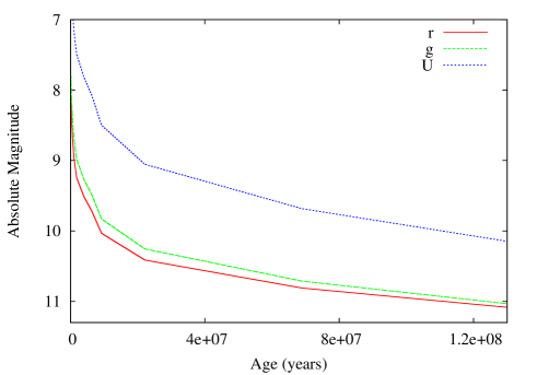
Figure 2: Age versus absolute magnitude for DA white dwarfs with $log(g)$=8 from Holberg $\&$ Bergeron (2006) for the UVEX $r$, $g$ and $U$ filter bands.

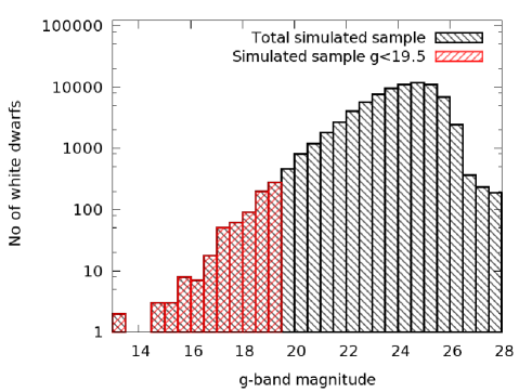
Figure 3: $g$-band magnitude histogram for the modelled white dwarf sample.

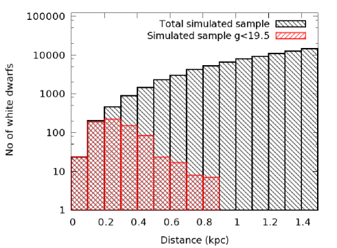
Figure 4: Distance histogram for the modelled white dwarf sample. The number white dwarfs brighter than $g<19.5$ decreases for distances larger than 0.25 kpc while the number of white dwarfs in the total simulated sample continues to increase.

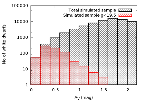
Figure 5: $A_{V}$ histogram for the modelled white dwarf sample.

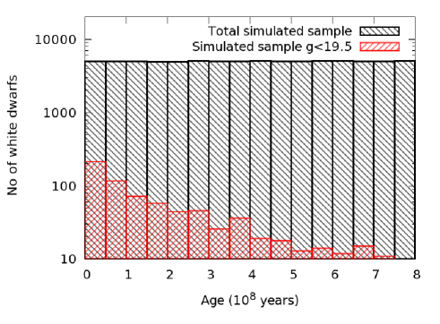
Figure 6: Age histogram for the modelled white dwarf sample. The number of white dwarfs brighter than $g<19.5$ decreases for older systems, the number of white dwarfs in the total simulated sample is constant for all bins due to the assumption of a constant birth rate.

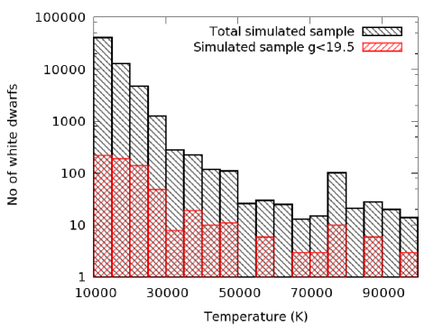
Figure 7: Temperature histogram for the simulated white dwarf sample.

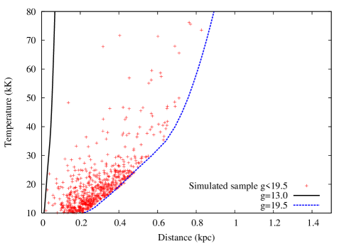
Figure 8: Temperature versus distance for the modelled white dwarf sample (red). The two lines indicate the survey limits at $g$=13 and $g$=19.5.

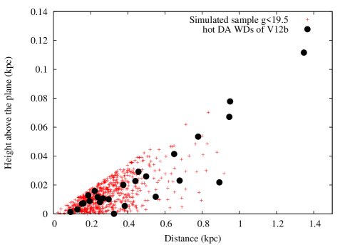
Figure 9: Height above the Galactic Plane versus distance for the modelled white dwarf sample (red) and the William Herschel Telescope (WHT) spectroscopically confirmed DA white dwarfs (black) of V12b.

2 A theoretical Galactic Model sample

In the determination of the white dwarf space density and birth rate, the observations will be compared to a Galactic model population that has been constructed and scaled to emulate the observations. The model is detailed in Nelemans et al. (2004) and is based on the Galaxy model according to Boissier $\&$ Prantzos (1999), including a Sandage (1972) extinction model. This model has been presented and used before in Nelemans et al. (2004), Roelofs, Nelemans & Groot (2007) and Groot et al. (2009). Note that for the simulated sample in this paper a constant white dwarf birth rate over the last 8$\times$10⁸ years is assumed. Only the spatial distribution of the white dwarfs comes from the model as described in Nelemans et al. (2004).

A theoretical sample of 8$\times$10⁴ DA white dwarfs is generated by a random distribution over ages 0-8$\times$10⁸ years and a model-weighted position in the Galaxy with a Galactic longitude spread of –180^∘$<$$l$$<$+180^∘, a Galactic latitude spread –5^∘$<$$b$$<$+5^∘(the limits of the EGAPS surveys), a distance $d$$<$1.5 kpc and an extinction $A_{V}$ appropriate to their distance and Galactic location.

Using the DA white dwarf cooling models by Wood (1995) the adopted age distribution ($<$8$\times$10⁸ years) translates into a minimal temperature of T_eff$>$9 000 K. This cut in temperature is required due to the uncertainties and incompleteness of colder white dwarfs in the observed sample (see Sect. 3). The temperature of the white dwarf is related to an absolute magnitude ($M$) for each filter band (Figs. 1 and 2). For each object, the absolute magnitude in the Vega system in the UVEX bands ($M_{U}$, $M_{g}$, $M_{r}$) has been calculated using the colour calculations of Holberg & Bergeron (2006), Kowalski & Saumon (2006), Tremblay et al. (2011) and Bergeron et al. (2011), assuming a surface gravity $\log g$ = 8.0, and the UVEX filter passbands presented in Groot et al. (2009). The magnitudes are converted to the Vega system using the AB offsets $U$=-0.927, $g$=0.103, $r$=-0.164 of González-Solares et al., 2008 and Hewett et al., 2006. These values need to be added to the AB magnitudes to convert them to the Vega system. Reddened apparent magnitudes and Vega colours for each white dwarf were calculated using $A_{\lambda}/A_{V}$=1.66, 1.16, 0.84 for the $U$-, $g$- and $r$-bands respectively. To emulate the observational sample of Sect. 3, only white dwarfs with $g$$<$19.5 were selected, keeping 723 systems out of the original model sample. The reason of the magnitude cut at $g$$<$19.5 is to warrant the completeness of the observational sample. Going deeper clearly showed a down-turn in the number of systems in the observational sample, indicative of loss of completeness.

The characteristics of the simulated white dwarf sample are shown in Figs. 3-9. Figure 3 shows that the number of white dwarfs keeps on increasing for magnitudes $g$$>$19.5 and only turns over around $g$$\sim$25 due to the combined effects of a minimum temperature and a limited volume in the model. White dwarfs detectable in a survey such as UVEX are only a tip of the iceberg compared to the total population, even within a limited distance of $\sim$1 kpc. No white dwarfs in the sample are brighter than $g$$\sim$13.3 and all white dwarfs brighter than $g$$<$19.5 are within $d$$<$0.92 kpc (Fig. 4). The observable sample is complete to a distance of $\sim$0.2kpc and all systems have extinctions smaller than $A_{V}$$<$1.7 (Figs. 4 and 5). $A_{V}$ peaks between 0.3 and 0.4 for the white dwarfs brighter than $g<19.5$ while it peaks between 1.7 and 1.8 for the total simulated white dwarf sample.

The age distribution is shown in Fig. 6, and the corresponding white dwarf temperatures in Fig. 7. The fraction of hot, young white dwarfs is larger than the fraction of older, colder white dwarfs. The number of white dwarfs in the complete simulated sample varies with different Galactic latitude and longitude. While the number of white dwarfs in the total simulated sample is higher at Galactic latitude $b$=0^∘ and Galactic longitude $l$=0^∘, the number in the $g$$<$19.5 sample is constant over Galactic latitude and Galactic longitude. The white dwarfs brighter than $g$$<$19.5 are equally distributed over different Galactic latitudes and Galactic longitudes due to the limited distance probed in this first, relatively shallow sample. The distributions over distance, temperature and height above the Galactic Plane of the numerical, observable sample are shown as red points in Figs. 8 and 9. The lines in Fig. 8 show for the chosen upper and lower magnitude limits in the observable out to which distance a survey such as UVEX is sensitive as a function of temperature.

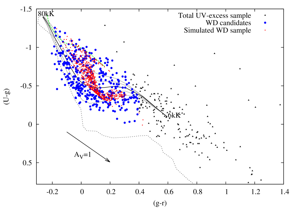
Figure 10: Colour-colour diagram with the UV-excess sources of V12a brighter than g$<$19.5 (black triangles), the white dwarf candidates in the UV-excess catalogue (blue circles), and the simulated white dwarf sample brighter than g$<$19.5 (red squares). Overplotted are the simulated colours of unreddened main-sequence stars (dashed black) and the simulated colours of unreddened Koester DA (solid black) and DB (dashed green) white dwarfs of V12a. The DA white dwarf colours are shown for different $log\,g$=7.0, 7.5, 8.0, 8.5, 9.0, where the upper line is $log\,g$=9.0. The DA white dwarf colours cover the range 80kK$>T_{\rm eff}>$6kK No photometric error bars are plotted for clarity, photometric errors range from 0.002 mag at $g$=16 to $<$0.025 mag at $g$=19.5. The simulated DA white dwarfs are distributed over the Galaxy and reddened to their Galactic position. The simulated sources around the unreddened DB track (dashed green) are reddened hot DA white dwarfs. The vector ($A_{V}$=1) shows the direction of the reddening, its length is equal to $A_{V}$=1.

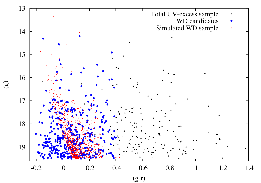
Figure 11: Colour-magnitude diagram with the UV-excess sources of V12a brighter than g$<$19.5 (black triangles), the white dwarf candidates in the UV-excess catalogue (blue circles), and the simulated white dwarf sample brighter than g$<$19.5 (red squares). No photometric error bars are plotted for clarity, photometric errors range from 0.002 mag at $g$=16 to $<$0.025 mag at $g$=19.5.

3 The Observational white dwarf sample

The UV-excess catalogue of V12a, selected from the first 211 square degrees of UVEX data contains 2 170 UV-excess sources. In the colour-colour and colour-magnitude diagrams an automated algorithm selects blue outliers relative to other stars in the same field. We have used recalibrated UVEX photometry to correct for the time-variable $U$-band calibration as noted in Greiss et al. (2012). The recalibrated UVEX data are explained in Appendix A.

Since we are interested in a complete sample of white dwarfs with minimal pollution we select all sources with $g$$<$19.5 and $(g-r)$$<$0.4. The distribution of the observational sample for magnitudes fainter than $g$$>$19.5 clearly showed a down-turn indicative of loss of completeness, therefore a magnitude cut at $g$=19.5 is applied. The colour cut at $(g-r)$$<$0.4, which corresponds to the colour of unreddened DA white dwarfs with $T_{\rm eff}$$\sim$7 000K, is applied since all DA white dwarfs in V12b have $(g-r)$$<$0.4 (Figs. 1 and 2 of V12b). From spectroscopic follow-up of V12b it is known that the observational sample with $(g-r)$$<$0.4 is dominated by DA white dwarfs, and spectroscopy of the “subdwarf sample” of V12a shows that the UV-excess catalogue is complete for white dwarfs. The effects of the pollution of the observational sample are corrected in Sect. 6. Additionally, sources more than 0.1 magnitude above the reddened white dwarf locus in the $(g-r)$ vs. $(U-g)$ colour-colour diagram are not taken into account since they are more than 0.1 magnitude above the reddened hottest white dwarf model.

These cuts result in an sample of 360 observed candidate white dwarfs, which will be used as the basis of the space density and birth rate calculations in this paper. The observational white dwarf sample is shown in the colour-colour and colour-magnitude diagrams of Figs. 10 and 11, overplotted by the simulated sample of Sect. 2. The objects in the simulated sample have colours similar to reddened synthetic colours shifted by a defined amount of reddening, determined by the Galactic position of the objects in the theoretical sample. The simulated white dwarf sample and the observed white dwarf sample have different colours since the observed sample has a photometric scatter and an uncertainty on the absolute calibration. Additionally, from V12b it is known that the observed sample contains some non-DA sources, such as DB white dwarfs. We correct for these non-DAs in Sect. 6.

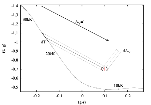
Figure 12: The temperature and reddening of each white dwarf in the observational sample are determined from the location in the colour-colour diagram. The temperature is determined by tracing the reddening vector (thick line) back to the unreddened synthetic $log\,g$=8.0 DA white dwarfs model colours of V12a. The reddening corresponds with the length of the reddening vector. The error on the determined temperature and reddening are related the photometric error and the error on the temperature depends on the position of the source in the colour-colour diagram.

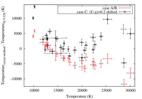
Figure 13: Difference between the temperature determined from the photometry by the vector method and the temperature determined through line profile fitting in V12b. When the vector method is applied to the original UVEX data (cases A and B) the difference in temperature increases for hotter white dwarfs with a clear trend. For the UVEX with a shift of $(U-g)$=0.2 magnitude (case C) the difference in temperature is more scattered around zero without this trend. There are two more hot white dwarfs at $35kK<T_{\rm eff}<40kK$ that have a temperature difference larger than 15kK.

4 Space densities and birth rates: Method

The method to derive the space density and birth rate is first to calculate for each system in the observational sample its current temperature and distance, and then to scale and compare the distribution of the observed sample to the simulated, numerical sample. Herein we adjust the space density of the numerical sample to match the observed number of systems. The test we perform here is therefore how well the observed population resembles a simulated, numerical sample. In Sect. 9 we will discuss the validity of our assumptions in constructing the numerical, observable sample.

To derive temperatures and distances the observed position of a source in the $(g-r)$ and $(U-g)$ diagram is compared with a grid of reddened model colours, based on the hydrogen dominated white dwarf atmosphere models of Koester et al. (2001) for temperatures in the range 6 000$\leq T_{\rm eff}$$\leq$80 000 K. We assume a fixed surface gravity of $\log g$ = 8.0, as this is the median value found in the spectroscopic fitting of a representative sample of the white dwarf systems in V12b (Fig. 5 of V12b, and e.g. Fig. 5 of Vennes et al., 1997; Fig. 9 of Eisenstein et al., 2006). The impact of this assumption of a fixed surface gravity of $\log g$ = 8.0 is discussed in Sect. 9. The reddening grid was calculated at $\Delta E(B-V)$=0.1 intervals. The best-fitting value for an individual system is taken as the grid point with the smallest distance to the observed value (see Fig. 12). Error estimates on the fit values are obtained by projecting the 1$\sigma$ photometric errors on to the grid axes, often resulting in asymmetric errors in temperature. The distance to a source is derived from the combination of the observed $g$-band magnitude, the model absolute magnitude corresponding to the surface gravity and the derived temperature, including the reddening value derived from the fit.

As the synthetic colour tracks of white dwarfs display a distinct ‘hook’ in the colour-colour plane at $T_{\rm eff}$=10 000K (Fig. 10), due to the strength of the Balmer jump, a highly reddened object may have a dual possible solution: a high temperature/high reddening, or a low temperature/low reddening solution. The numerical model shows that in most of the cases where a dual solution exists, the preferred one is the hot solution. In observational samples cool white dwarfs below $T_{\rm eff}$$<$10 000K are more rare (Fig. 5 V12b, Eisenstein et al., 2006 and Finley et al., 1997). Therefore it is assumed that in all cases the hot solution is correct. The impact of this assumption will be discussed in Sect. 9.

Fig. 10 shows the colour-colour diagram of the selected UVEX sample alongside theoretical tracks of cooling white dwarfs of various surface gravity ($\log g$ = 7.0 - 9.0, from bottom to top). The spectroscopic analysis of V12b (Fig. 5) shows that the vast majority of the DA white dwarfs in the UVEX sample have $\log g$$\sim$8, and should therefore lie at the $\log g$=8 line. However, a substantial number of systems in Fig. 7 of V12b lie below the line, either due to their own photometric error, the scatter in the absolute calibration in the $U$-band magnitude, the lack of a global photometric calibration in the UVEX survey, or a combination of all three. To investigate the effect of this scatter on the determination of the space densities and birth rates three separate samples are defined and analysed.

• Sample A (only systems above $\log\,g$=8.0 line): In sample A, 84 white dwarfs which are located far under/left of the unreddened synthetic $\log\,g$=8.0 colour track of Fig. 10 are not taken into account. To allow for some intrinsic photometric scatter all systems that lie closer than 0.1 magnitude left of the unreddened synthetic $\log\,g$=8.0 colour track are included, automatically have reddening $E(B-V)$=0, and are assigned the temperature of the grid point on the track most closely located to the measurement. Sample A contains 276 white dwarf systems.
  

• Sample B (all systems): In sample B all candidate white dwarfs shown in Figs. 10 and 11 are included. Temperatures and reddening vectors are compared to $\log g$=8.0 models only. For systems below the $\log g$=8.0 line, temperatures and reddenings are assumed to be those of the closest grid point on the $\log g$=8.0 line. This sample will correctly include the number of systems present, but will overestimate the number of systems at very low reddenings. Sample B contains 360 systems in our footprint.
  

• Sample C (shifted $U$-band): In sample C a shift of $(U-g)$=–0.2 is applied to all systems in the observational sample. This brings the vast majority of systems above the $\log g$=8.0 line. The magnitude of the shift is the maximum scatter observed in the $U$-band calibration and will therefore in general overestimate the actual calibration uncertainty. A consequence of the $(U-g)$ shift is that each white dwarf will get a different colour, and so a different $T_{\rm eff}$, $E(B-V)$ and distance. Sources that are more than 0.1 magnitude above the white dwarf grid after the colour shift are not taken into account. This sample excludes a fraction of systems and will lead to an overestimate of the number of hot, distant systems. Sample C contains 303 systems in our footprint.
  

Note that samples A and C do not give the best exact value of the space density and birth rate, but are presented to show the effect of a colour shift or cut $\log g$$>$8. To obtain a feel for the accuracy in temperature and reddening from the photometric method, the effective temperature ($T_{\rm eff}$), surface gravity ($\log g$) and reddening of the 20 UVEX white dwarfs with $T_{\rm eff}$$>$20 000K in V12b (Table 2, Fig. 5) were compared with the photometric method, with and without applying any shifts, and the results are shown in Fig. 13. For samples A and B, the difference in effective temperature found by the photometric method and determined through line profile fitting of V12b appears to increase for hotter white dwarfs. This trend is less clear for sample C, see Fig. 13.

In the photometric method the error on the temperature depends on the $(g-r)$ and $(U-g)$ colours of the white dwarf. The errors on the temperature and reddening due to the method are between $\Delta T_{\rm eff}$=2 000K for white dwarfs of $T_{\rm eff}$=25 000 K and $\Delta T_{\rm eff}$=15 000K for white dwarfs of $T_{\rm eff}$=60 000 K and $\Delta E(B-V)$$\sim$0.03 for sources with a photometric error of $\Delta g$=0.01 mag. However, the uncertainty in temperature and reddening is larger because of the lack of a global photometric calibration.

Photometric distances ($d$) to all systems in the observed samples were calculated using

$$d=0.01\times 10^{0.2(m_{g}-M_{g}-A_{g})}(kpc)$$

, where $m_{g}$ and $M_{g}$ are the observed and absolute $g$-band magnitude and $A_{g}$ is the extinction in the $g$-band. The absolute magnitudes of Holberg & Bergeron (2006) are used, assuming $\log g$=8.0 for all white dwarfs.

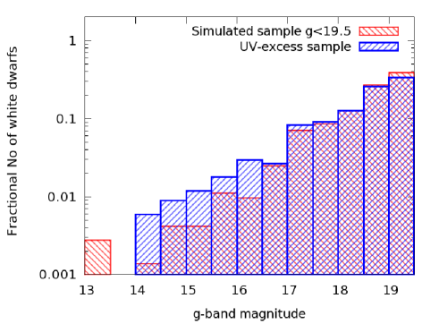
Figure 14: Histogram of g-band magnitudes of the UV-excess white dwarf candidates of sample B and the simulated white dwarf sample.

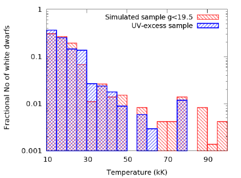
Figure 15: Temperature histogram of the UV-excess candidate white dwarfs of sample B and the simulated white dwarf sample.

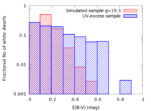
Figure 16: Histogram of $E(B-V)$ of the UV-excess candidate white dwarfs of sample B and the simulated white dwarf sample.

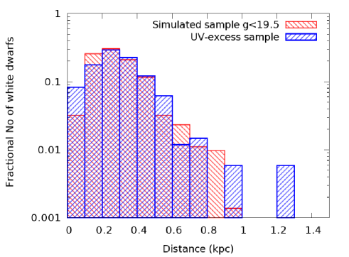
Figure 17: Distance histogram of the UV-excess candidate white dwarfs of sample B and the simulated white dwarf sample.

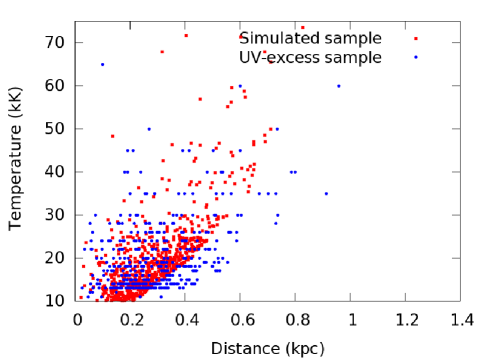
Figure 18: Temperature versus distance of the UV-excess candidate white dwarfs (sample B) from UVEX (blue) and the simulated sample (red).

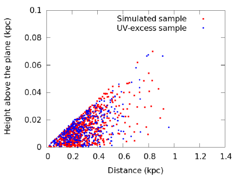
Figure 19: Height above the plane versus distance of the UV-excess candidate white dwarfs (sample B) from UVEX (blue) and the simulated sample (red).

5 Results

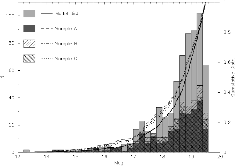
Figure 24: Magnitude distributions and cumulative distributions of the UV-excess white dwarf candidates from the 3 samples A-C and the simulated white dwarf sample.

For illustration purposes only the distribution comparisons for sample B are shown here (Figs. 14 to 17). The histograms of all three samples (A-C) are shown in Figs. 24 to 27 of Appendix B. For the magnitude, reddening, distance and temperature distributions, sample B is most consistent with the simulated sample. Because sample B is most complete and has the best Kolomogorov-Smirnov (KS) results, this sample will be emphasized in the next sections.

Table 1: KS tests between the derived, observed, and numerical distributions for samples A-C.

Distribution	Sample A	Sample B	Sample C
	$(D,p)$	($(D,p)$	$(D,p)$
Magnitude	(0.09,0.07)	(0.08,0.11)	(0.09,0.09)
Reddening	(0.40,4.0$\times$10-26)	(0.30,1.2$\times$10-18)	(0.41,9.6$\times$10-30)
Distance	(0.07,0.25)	(0.06,0.49)	(0.22,1.2$\times$10-8)
Temperature	(0.20,6.2$\times$10-7)	(0.17,3.0$\times$10-6)	(0.36,1.1$\times$10-22)

To test whether the distributions in temperature, distance and reddening between the observational and numerical sample are consistent with each other, a KS test was performed on the cumulative distributions in magnitude, reddening, distance and temperature, with limiting values of 13$<$$g$$<$19.5, 0$<$$E(B-V)$$<$0.7, 0$<$$d$(kpc)$<$1.0 and 10 000$<$$T$(K)$<$ 80 000. The results of the KS-test are summarized in Table 1. The D-value is the maximum distance between the cumulative distributions and the p-value is the probability that the observational and numerical samples are the same distributions. If the D-value is small or the p-value is high, the hypothesis cannot be rejected that the distributions of the numerical and observational samples are the same.

Our main conclusion from Table 1 and the distributions shown in Figs. 14 to 17 is that the numerical sample reproduces the reconstructed observational samples reasonably accurate, except for the reddening and temperature, where, for sample B, the reddening gradient is too shallow. There are not enough observed systems at low reddening, and too many at high reddening. Note however, that the model reddening is a very simple Sandage-type relation and can therefore easily underestimate the amount of reddening in the local volume.

Figs. 18 and 19 show the main similarities and differences between the observed white dwarf sample and the theoretical $g$$<$19.5 sample. In Fig. 18 there is a clear lower limit in the distance-temperature distribution due to a linear relation between the distance and reddening for the theoretical white dwarfs, while there are candidate white dwarf in the observational sample that have little reddening at a large distance or strong reddening at a small distance as a result of the method in Sect. 4. Note that due to the method of Sect. 4 the results of $T_{\rm eff}$ and $E(B-V)$ are strongly correlated. All white dwarfs have a height above the plane smaller than 0.07 kpc (Fig. 19), which is a consequence of the UVEX Galactic latitude limit $|b|$$<$5^∘, and all white dwarfs are within a distance of 1.0 kpc due to the brightness limit of UVEX .

The vector method finds several solutions at $T_{\rm eff}$=80kK since that is the hottest model of the white dwarf grid, see Fig. 15. A small fraction of these sources might be photometrically scattered DA white dwarfs, white dwarfs hotter than $\Delta T_{\rm eff}$$>$80 000K, non-DA white dwarfs (DB, DA+dM) or subdwarfs. As shown in V12b and follow-up spectroscopy of the comparable region in the Sloan Digital Sky Survey (Rau et al., 2010; Carter et al., 2012, and V12b), the majority of these objects are helium-line (DB) white dwarfs, subdwarfs, DA+dM stars and Cataclysmic Variables. These hottest solutions also induce the peaks at 0.8$<$$E(B-V)$$<$0.9 and 1.2$<$$d(kpc)$$<$1.3 in Figs. 16 and 17.

The maximum reddening of $E(B-V)$=0.7 in Fig. 16 corresponds with a maximum extinction of $A_{V}$=2.2 using $R_{V}$=3.1 and is in agreement with Fig. 8 of V12b. The difference between the theoretical and observational sample for reddening smaller than $E(B-V)$$<$0.2 might be due to the method to determine the temperature and reddening of the UV-excess sources below the unreddened white dwarf track. The method assumes the nearest grid point for these sources while these sources might be slightly more reddened in reality.

6 Completeness of the observed sample

Before space densities and birth rates can be derived by scaling the observed sample to the numerical sample, a number of corrections to the observed sample need to be applied:

6.1 Non-DA white dwarf selection

In the spectroscopic follow-up of the UV-excess catalogue presented in V12b, it was concluded that 67$\%$ of the sources with $g$$<$19.5 and $(g-r)$$<$0.4 were indeed DA white dwarfs (Fig. 1 and Fig. 2 of V12a). Fifteen percent was classified as white dwarfs of other types (DB, DAB, DC, DZ, DA+dM, DAe) and 18$\%$ were non-white dwarfs (Cataclysmic Variables, Be stars, sdO/sdB stars). For a correct derivation of the space number density and birth we correct for the fraction of genuine DA white dwarfs and take the 67$\%$ into account. This is the largest correction made to the observed numbers.

6.2 Non-selection of DA white dwarfs

From spectroscopic follow-up of the ‘subdwarf sample’ (see V12a) it is concluded that the method described in V12a selects all observable white dwarfs, so the observational sample is almost complete in its selection of white dwarfs with temperatures $T_{\rm eff}$$>$10 000K ($M_{V}$$<$12.2). In both the theoretical and observational samples, only white dwarfs hotter than $T_{\rm eff}$$>$10 000K are taken into account, due to the distinct ‘hook’ in the synthetic colours of white dwarfs in the $(U-g)$ vs. $(g-r)$ colour-colour diagram The brightest UV-excess candidates with $g$$<$16 and $(g-r)$$<$0.4 have a chance not to be selected, see Fig. 14 of V12a. The sources brighter than $g$$<$16 are a small fraction of only 2$\%$ of the theoretical sample and 3$\%$ of the observational sample. Additionally, in the simulated white dwarf sample there are 3 sources with $(g-r)$$>$0.4, so some reddened white dwarfs could be missed in the observational sample because they are at $(g-r)$$>$0.4. For the derivation of the space number density and birth, these effects are not taken into account, since both contributions are negligible.

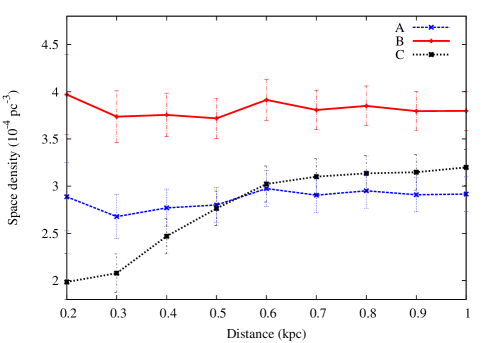
Figure 20: Space density versus distance for the three different samples (A, B, C), demonstrating that the space densities derived only slightly depend on the volume. Here the error bars indicate the number of white dwarfs ($N$) used to derive each space density and are calculated as $1/\sqrt{(}N)$.

Table 2: Space densities for DA white dwarfs with $T_{\rm eff}>$10 000K and birth rates from UVEX .

Case	Space density $(10^{-4}pc^{-3})$	Birth rate $(10^{-13}pc^{-3}yr^{-1})$	Caveats
A	2.9 $\pm$ 0.8	5.4 $\pm$ 1.5	Not complete
B	3.8 $\pm$ 1.1	5.4 $\pm$ 1.5	Too many $E(B-V)$=0
C	3.2 $\pm$ 0.9	7.3 $\pm$ 2.0	Too many hot/young, not complete

7 Derivation of the space number density of DA white dwarfs from UVEX

The observed white dwarf sample from UVEX is selected from 211 square degrees along the Galactic Plane. The simulated numerical sample is obtained from the full Galactic Plane (3 600 square degrees). Since the sample with $g$$<$19.5 shows no longitude or latitude dependence, the area ratio between the observed sample and the simulated sample is simply a factor 211/3 600. Assuming equal depths of 1.0 kpc, the volume of the simulated white dwarf sample is $0.365$ kpc³ and the observed white dwarf sample is the same factor 3600/211 times smaller.

The observed UV-excess samples (A, B, C) contain (276,360,303) sources and the simulated sample contains 723 white dwarfs in the full Plane. If we correct the observed sample for the fraction of genuine DA white dwarfs (67$\%$), there are (185,241,203) DA white dwarf candidates in a volume within 1.0 kpc. If we correct the volume of the observed sample there would be $723\times$ (211/3 600)=42.4 times more theoretical white dwarfs in the volume. The difference between the number of observed white dwarfs and number of simulated white dwarfs is a factor (185,241,203)/42.4 = (4.36,5.68,4.79) for cases (A, B, C).

Using these ratios to scale the observed sample to the total numerical sample of $8\times 10^{4}$ white dwarfs with $T_{\rm eff}$$>$10 000K, an average space density in a volume within a radius of 1 kpc around the Sun is obtained of $\overline{\rho_{A}}$ = 2.9 $\pm$ $0.8\times 10^{-4}$ pc^-3, $\overline{\rho_{B}}$ = 3.8 $\pm$ $1.1\times 10^{-4}$ pc^-3 and $\overline{\rho_{C}}$ = 3.2 $\pm$ $0.9\times 10^{-4}$ pc^-3. These results are summarized in Table 2. The derivation of the errors here is explained in Sect. 9.

To test the validity of the model assumption on Galactic reddening, and to test the sensitivity of the result as a function of the actual distance/volume used in the calculations, the cut-off distance has been varied between 0.1 and 1.0 kpc in steps of $\Delta d$=0.1 kpc. The resulting average space densities are shown in Fig. 20, which shows that the result is very stable in the range 0.6 - 1.0 kpc. Below 0.5 kpc the results change rapidly, both within one sample as well as between the three samples. This is caused by low number statistics, combined with the relatively large uncertainties on individual systems, inherent to the photometric method of deriving temperatures and reddenings.

Figure 21: The UVEX birth rate of sample B for different limits of $T_{\rm eff}$. The error bars, indicating the number of white dwarfs ($N$) used for each birth rate, are calculated as $1/\sqrt{(}N)$.

8 Birth rate of DA white dwarfs in the Galactic Plane

For the derivation of the birth rate of DA white dwarfs, only objects with $T_{\rm eff}$$\geq$20 000K are taken into account. The samples are limited to $T_{\rm eff}$$\geq$20 000K since for the hottest systems the cooling tracks is less uncertain (see Fig. 1) and the assumption of a constant birth rate is more realistic, while for a higher $T_{\rm eff}$ the number of systems in the samples would become too small. From the cooling tracks of Fig. 1 we assume that all white dwarfs in the samples with $T_{\rm eff}$$\geq$20 000K are younger than $\sim 6.9\times 10^{7}$ years. From the 211 square degrees of V12a there are (153,154,211) white dwarf candidates with $T_{\rm eff}$$\geq$20 000K for samples A, B and C of Sect. 4, respectively, taking the 67$\%$ into account. This area of 211 square degrees has a volume of 2.14 $\times$ 10^-3 kpc³ using a depth of 1.0 kpc.

Within the full numerical sample there are 2 024 white dwarfs with $T_{\rm eff}$$\geq$20 000K within 1.0 kpc, of which 267 have a magnitude $g$$<$19.5 and fall within the simulated sample. If we correct for the volume and the ratio between simulated and observed sources the same way as in Sect. 7, the birth rate for the samples A, B and C is (5.4 $\pm$ 1.5) $\times$ 10^-13 pc^-3yr^-1, (5.4 $\pm$ 1.5) $\times$ 10^-13 pc^-3yr^-1 and (7.3 $\pm$ 2.0) $\times$ 10^-13 pc^-3yr^-1. These results are summarized in Table 2. The derivation of the errors here is explained in Sect. 9.

So far the birth rate is derived using the samples limited to $T_{\rm eff}$$\geq$20 000K. Fig. 21 shows that birth rate varies between 2.5 $\times$ 10^-13 pc^-3yr^-1 and 6.7 $\times$ 10^-13 pc^-3yr^-1 for different limits of $T_{\rm eff}$. However, the birth rates at $T_{\rm eff}$$\geq$26 000K are influenced by the shape of the cooling tracks and the age versus absolute magnitude relation (Fig. 2), while the birth rates at the higher temperatures are affected by low number statistics.

9 Discussion and conclusions

A derivation of the average space density and birth rate within a radius of 1 kpc around the Sun very much depends on the ability to construct volume-limited samples, to estimate the completeness and biases in the observational sample, and the accuracy of deriving fundamental parameters from observational characteristics. As outlined in Sect. 5, the space densities have been estimated using three observational samples, each with its own set of biases and/or corrections. Sample A is a conservative lower limit, since this sample excludes white dwarfs left from the unreddened $\log g$=8.0 colour track in the colour-colour diagram. In sample B all white dwarfs are taken into account, so the space density derived from this sample is the most complete, however, the method overestimates the number of systems with no reddening. For sample C the space density is also a lower limit, since the sample excludes a fraction of systems above the grid, while the derived birth rate is too large due to an overestimate of the number of hot/young systems.

A number of caveats and limitations are in common between the three samples. The estimated space density depends on: (i) the distance determination, (ii) uncertainties in the method for estimating the temperature and reddening of the white dwarfs in the observational sample, (iii) the assumption about the amount of reddening/extinction, (iv) the magnitude cut $g$$<$19.5, (v) the colour cut $(g-r)$$<$0.4, (vi) the assumption of $\log g$=8.0 for all white dwarfs, (vii) the fraction of genuine white dwarfs in the UV-excess catalogue and (viii) the binary fraction in the UV-excess catalogue. The estimated white dwarf birth rate depends on these points as well, with the additional assumptions about the cooling time and constant birth rate.

The distance estimates to individual systems strongly depend on the assumed absolute $g$-band magnitudes from Holberg & Bergeron (2006), assuming $\log g$=8.0 for all white dwarfs. The absolute magnitudes follow from the temperature and reddening determined from the UVEX photometry. If the absolute magnitude would be brighter than derived, the white dwarfs would be detectable over a larger volume. In the most extreme cases, for example due to a maximal shift in $(U-g)$ of –0.2 magnitudes, the temperature determinations are off by $\Delta T_{\rm eff}$=+6 000K for cool white dwarfs and up to $\Delta T_{\rm eff}$=+30 000K for the hottest white dwarfs. The surface gravity determination could be off by $\Delta\log g$=0.5 (Fig. 5 of V12b). We note that although in the last case we would strongly overestimate an absolute bolometric magnitude, the effect is ameliorated by the fact that the change in the absolute $g$-band magnitude is less severe at these very hot temperatures. In these cases the absolute magnitude would be overestimated by $M_{g}$$\sim$1 magnitude on an individual basis. If the apparent magnitude of a source at 1.0 kpc would change by $m_{g}$=0.1 magnitude, the distance would typically change by 5$\%$. If this would be the case for the total sample, this would mean a maximal increase or decrease of 15$\%$ of the total survey volume. There might be a Malmquist-type bias in the distance-selected observational sample. There will be distance uncertainties since the observational sample will include white dwarfs which are outside the chosen distance limit, but brought in because of distance errors, and it will exclude objects which are moved to outside of the distance limit because of distance errors. There is no direct effect since the observational sample is compared to the simulated sample, and the space densities, calculated using different volumes in Fig. 20, depend only slightly on the volume. For the derivation of an error on the space number density (see below), the effect of this bias is taken into account within the factor of 15 per cent of the photometric scatter.

The colour cut $(g-r)$$<$0.4 and the magnitude cut $g$$<$19.5 will cause a loss of systems on the total number of white dwarfs in the observational sample. In the simulated sample there are three white dwarfs with $(g-r)$$>$0.4 and $g$$<$19.5: a fraction of $\sim$0.4$\%$, negligible compared with the other correction factors applied (see Fig. 14). In the observed UV-excess sample there are no sources with $(g-r)$$>$0.4 spectroscopically confirmed as white dwarfs in V12b. The probability that a source with $g$$<$19.5 and $(g-r)$$<$0.4 will be picked-up by the selection algorithm (Fig. 14 of V12a) drops for sources brighter than $g$=16 and redder than $(g-r)$$>$0.2 to $\sim$50$\%$. Unreddened white dwarfs cooler than $T_{\rm eff}$$<$7 000K have synthetic colours $(g-r)$$>$0.4, due to the colour cut the final white dwarf sample is incomplete for these cool white dwarfs. However, in the comparison with the numerical model these cool dwarfs have also been excluded, and their exclusion from the observational sample therefore does not influence the estimate on the space density of hotter white dwarfs (T$>$10 000 K).

The magnitude cut at $g$$<$19.5 is applied due to the difference between the magnitude distributions of the simulated sample and the observational samples for magnitudes fainter than $g$$>$19.5. For fainter magnitudes the number of white dwarfs in the simulated sample increases strongly while the number of white dwarfs in the observational sample starts to drop. For magnitudes $g$$>$19.5 the observational sample is not complete which would influence the result of the space density. If a magnitude limit of $g$$<$20.0 was chosen, the space densities would have been (2.4 $\pm$ 0.7) $\times$ 10^-4 pc^-3, (3.2 $\pm$ 0.9) $\times$ 10^-4 pc^-3 and (2.7 $\pm$ 0.8) $\times$ 10^-4 pc^-3 for the three samples (A, B, C), which is $\sim$16$\%$ smaller.

The UV-excess catalogue was selected from 726 partially contiguous‘direct’ fields, as defined in González-Solares et al. (2008). Because of the tiling pattern of the IPHAS and UVEX surveys a completely contiguous area of this number of fields would result in an overlap in area of $<$5$\%$, which is the maximal correction on the 211 square degree area that could be applied. Over the covered area a number of sources might be missed because they fell on dead pixels or very near the edges of the CCDs. However, the WFC consists of high quality CCDs and the total dead area is $<$1$\%$.

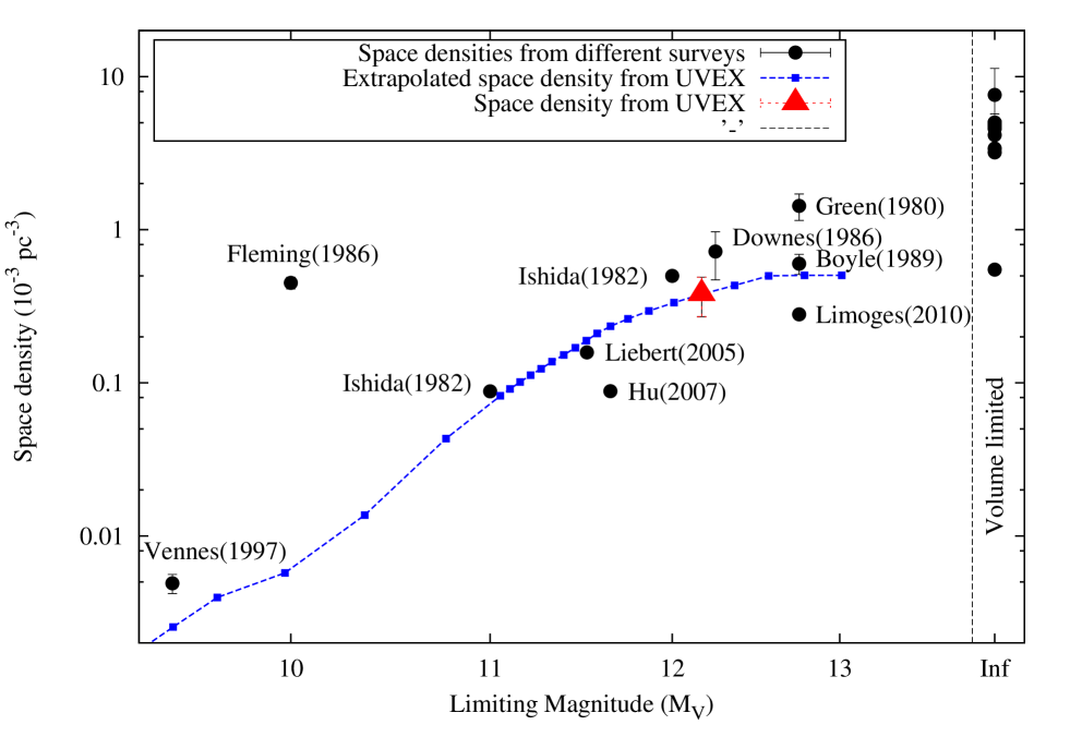
Figure 22: The UVEX space density of sample B (blue squares) extrapolated for different $M_{V}$ overplotted on the space number densities from other surveys (black dots). The dots at “Inf” represent the space densities of the volume limited surveys indicated in Table 3.

An assumption that may strongly affect the estimates is the assumption of $\log g$=8.0 for all sources. This has been motivated by the findings in V12b (Fig. 5) and the well known strong biases in previous studies of the white dwarf population towards $\log g$=8.0 (e.g. Fig. 5 of Vennes et al., 1997 and Fig. 9 of Eisenstein et al., 2006.). At face value Fig. 10 suggests that in the Plane a substantial number of sources exist with $\log g<8$, although this is not substantiated by the spectroscopic fitting in V12b. However, if a large number of lower gravity systems are present, this would lead to an overestimate of the space density since lower gravity systems are more luminous at a given temperature and the observed sample therefore occupies a larger volume. At a given temperature $\log g$=7.5 gravity white dwarfs will have larger absolute magnitudes of $\sim$ 0.8-0.9 mag compared to $\log g$=8.0 of DA white dwarfs. Their distance would be underestimated, and so also the space density would be overestimated by a factor of $\sim$25$\%$. For the derivation of an error on the space number density (see below), an error on the surface gravity of $\Delta\log g$=0.1, which is a typical value of the scatter in the white dwarf surface gravity (Fig. 5 of V12b), will be taken into account.

Combining the uncertainties mentioned above leads to an upper and lower limit on the space number density derived in Sect. 7. If we consider the most optimistic case, the upper limit is due to a combination of the method of Sect. 4 and photometric scatter of 0.5 mag (15$\%$), an error of $\Delta\log g$=0.1 (6$\%$) non-selected DA white dwarfs at $(g-r)$$>$0.4 (1$\%$), non-selected by the algorithm of V12a (1$\%$) (see Sect. 6.2) and non-selected white dwarfs due to tiling of the fields and errors on the CCD chips (5$\%$). The error on the birth rate is estimated in a similar way as for the space density. If the same uncertainties are taken into account, the birth rate would be 28$\%$ larger in the most optimistic case. Now for sample C, the distributions are less similar to the modelled theoretical sample, and the method finds too many hot solutions. For this reason the birth rate for sample C is larger than for sample B.

Table 3: Space number densities from other surveys.

Reference	Space density $(10^{-3}pc^{-3})$	Limits
UVEX	0.38$\pm$0.11	$M_{V}<12.2$
Giammichele (2012)∗	4.39	local
Limoges (2010)	0.280	$M_{V}<12.75$, DA WDs in Kiso
Limoges (2010)∗	0.549	All $T_{\rm eff}$ in Kiso DA WD sample
Sion (2009)∗	4.9$\pm$0.5	local, 20 pc
Holberg (2008)∗	4.8$\pm$0.5	local, 13 pc (122 WDs)
Holberg (2008)∗	5.0$\pm$0.7	HOS sample
Hu (2007)	0.0881	531 SDSS DA WDs, $12kK<T_{\rm eff}<48kK$ ($M_{V}<11.65$)
Hu (2007)	1.94	531 SDSS DA WDs, $T_{\rm eff}<48kK$
Harris (2006)∗	4.6$\pm$0.5	local
Liebert (2005)	0.158	$T_{\rm eff}>13kK$ ($M_{V}<11.52$)
Holberg (2002)∗	5.0$\pm$0.7	local, 13 pc
Knox (1999)∗	4.16	local, PM survey
Tat (1999)∗	4.8	local, 15 pc
Leggett (1998)∗	3.39	local, $1/V_{max}$
Vennes (1997)	0.019$\pm$0.003	EUVE sample of 110 DA WDs
Vennes (1997)	0.0049$\pm$0.0007	hot DA WDs $T_{\rm eff}>40kK$ ($M_{V}<9.45$)
Oswalt (1996)∗	7.6$\pm$3.7	local, wide binaries
Weidemann (1991)∗	5	local, in 10pc
Boyle (1989)	0.60$\pm$0.09	$M_{V}<12.75$
Liebert (1988)∗	3.2	local, $1/V_{max}$
Downes (1986)	0.72$\pm$0.25	$M_{V}<12.25$
Fleming (1986)	0.45$\pm$0.04	$M_{V}<10$, PG WD sample: 353 obj.
Shipman (1983)∗	4.6	local, astrom. binaries
Ishida (1982)	0.088	$M_{V}<11.0$, 588 KUV obj.
Ishida (1982)	0.500	$M_{V}<12.0$, 588 KUV obj.
Green (1980)	1.43$\pm$0.28	$M_{V}<12.75$
Sion (1977)∗	5	local, 23 WDs in 10 pc
∗ Volume limited

Table 4: Birth rates from other surveys.

Reference	Birth rate $(10^{-13}pc^{-3}yr^{-1})$	Limits
UVEX	5.4$\pm$1.5	$T_{\rm eff}>20kK$
Frew (2008)	8$\pm$3	PN birthrate
Hu (2007)	2.579	$12kK<T_{\rm eff}<48kK$, 531 SDSS DA WDs
Hu (2007)	2.794	$T_{\rm eff}<48kK$, 531 SDSS DA WDs
Liebert (2005)	6	PG WD sample: 348 obj.
Liebert (2005)	10$\pm$2.5	overall, in local disk
Holberg (2002)	6	over 8 Gyr
Phillips (2002)	21	local PN birth rate
Vennes (1997)	8.5$\pm$1.5	local
Pottach (1996)	4-80	local PN birth rate
Weidemann (1991)	23	derived from star/WD formation model
Boyle (1989)	$\sim$6	derived WD birth rate
Boyle (1989)	$\sim$20	obs. PN birthrate
Ishida (1987)	80	local PN birth rate
Green (1980)	20$\pm$10	from $M_{V}<12.75$ sample
Koester (1977)	20	from $M_{bol}<15.5$ sample

Fundamentally the analysis discussed here tests how well the numerical Galactic model resembles the observed distribution of white dwarfs. The Galactic model includes an idealized dust distribution that may not resemble the actual distribution. Since UVEX observes directly in the Galactic Plane in blue colours, the effect of the dust distribution and the ensuing reddening may be substantial. The theoretical dust distribution in the Sandage model may behave different than the actual distribution in our pointings, also because we are looking at a local population, while the extinction on exactly this local scale is very poorly known (Sale et al., 2009 and Giammanco et al., 2011). As can be seen in Fig. 16 there is a difference between the reddening distributions, which is partly due to the crude determination of $E(B-V)$ for the observational sample, with bins of $\Delta E(B-V)$=0.1. The effect of reddening for the white dwarfs in UVEX was already shown in Fig. 8 of V12b. The reddening is smaller than $E(B-V)$=0.7 ($A_{V}$$<$2.2) for all white dwarfs as shown in Fig. 16 and Fig. 8 of V12b. In the simulated observable sample there are no sources with $E(B-V)$$>$0.7. The most reddened white dwarfs have $E(B-V)$=0.55. In the observational sample the reconstruction method of Sect. 4 finds $E(B-V)$=1.0 and $T_{\rm eff}$=14kK for only one source, five sources with $T_{\rm eff}$$>$40kK have $E(B-V)$=0.7 and all other sources have $E(B-V)$$<$0.7.

When the local population of white dwarfs is well-known and spectroscopically characterized it can conversely be used to derive a 3D extinction map of the local ($d<1$kpc) environment.

Finally, we note that no correction has been made for the binary fraction of systems dominated by a DA white dwarf in the UV-excess catalogue. The binary fraction estimates range from 12$\%$ to 50$\%$ (e.g. Nelemans et al., 2001, Han 1995, Miszalski et al., 2009 and Brown et al., 2011). The space density and birth rate number derived here are therefore DA white dwarf dominated systems that fall within our colour selection criteria, including an unknown binary fraction.

9.1 Comparison with other surveys

The space density of (3.8 $\pm$ 1.1) $\times$ 10^-4 pc^-3, derived for sample B for white dwarfs with $M_{V}$$<$12.2 or $T_{\rm eff}$$>$10 000K, and a birth rate of (5.4 $\pm$ 1.5) $\times$ 10^-13 pc^-3yr^-1 over the last 7$\times$10⁷ years, can be compared with the results of other surveys (Tables 3 and 4). All previous estimates have been obtained either from bright samples (in particular the early surveys) and/or at high Galactic latitudes. The current study is the first to be obtained in the Galactic Plane itself where the majority of systems resides. For that reason, and due to different magnitude limits, it is not possible to automaticaly compare different surveys. As is evident from Tables 3 and 4, the estimates on the space densities and birth rates strongly vary. To compare our results to those of the other studies, the Galactic model is used to calculate the effective space density at various limiting magnitudes, calibrated to our result. Fig. 22 shows that, when a correction is made for the vaying limiting absolute magnitude, many surveys are quite consistent with each other, despite the fact that they observe different white dwarf samples. Surveys that claim to be volume limited derive an average space density of $\sim$4.6 $\times$ 10^-4 pc^-3, which is consistent with the extrapolated, continued slope of the space density as a function of absolute magnitude of Fig. 22. However, it is not possible to extrapolate the UVEX -based result to the coolest/faintest systems since the star formation history in the Galaxy will start to play a dominant role. For the same reason also the birth rate results of the different surveys in Table 4 strongly vary. If we compare the birth rate of 5.4 $\pm$ 1.5 $(10^{-13}pc^{-3}yr^{-1})$, derived for sample B in this paper, the result of UVEX is consistent with other estimates.

Appendix A Recalibrated UVEX data.

There is a possible systematic shift in the original UV-excess catalogue $(U-g)$ data, which would influence the result of methods in Sect. 4. For that reason we use recalibrated UVEX data, as explained in Greiss et al. (2012). The differences in $(U-g)$ between the original UVEX data and recalibrated UVEX data for the 5 different months used in V12a are plotted in Fig. 23. The shift in the original UVEX data does not influence the content of the UV-excess catalogue because the selection in V12a was done relative to the reddened main-sequence population. The magnitudes and colours of the UV-excess sources might still show a small scatter, similar to the early IPHAS data (Drew et al., 2005), since a global photometric calibration is not applied to the UVEX data yet.

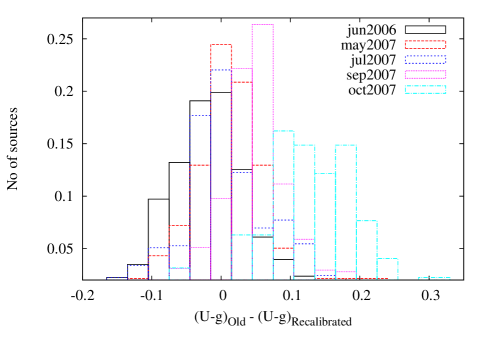
Figure 23: Difference in $(U-g)$ between the original UVEX data and recalibrated UVEX data for the 5 different months used for the UV-excess catalogue of V12a.

Appendix B Distributions of simulated and observational samples

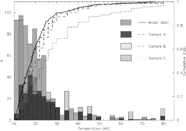
Figure 25: Temperature distributions and cumulative distributions of the UV-excess white dwarf candidates from the 3 samples A-C and the simulated white dwarf sample.

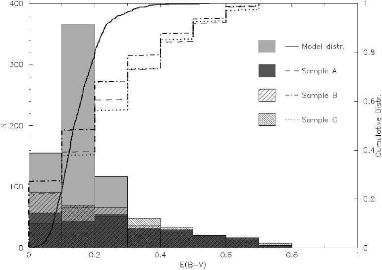
Figure 26: Reddening distributions and cumulative distributions of the UV-excess white dwarf candidates from the 3 samples A-C and the simulated white dwarf sample.

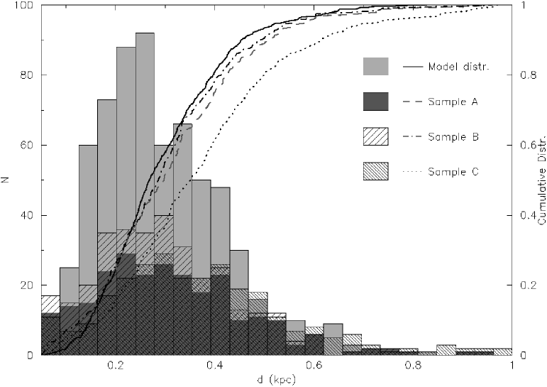
Figure 27: Distance distributions and cumulative distributions of the UV-excess white dwarf candidates from the 3 samples A-C and the simulated white dwarf sample.

References

- Aungwerojwit et al. (2005) Aungwerojwit A., Gänsicke B.T., Rodriguez-Gil P., et al., 2005, A&A 443, 995A
- Bahcall & Soneira (1980) Bahcall J.N. & Soneira R.M., 1980, ApJS 44, 73B
- Barentsen et al. (2011) Barentsen G., Vink J.S., Drew J.E., Greimel R. et al., 2011, MNRAS 415, 103B
- Becker et al. (1990) Becker R.H., White R.L., McLean B.J., Helfand D.J. & Zoonematkermani S., 1990, ApJ 358, 485B
- Bergeron et al. (1992) Bergeron P., Saffer R.A., Liebert J., 1992, ApJ 394, 228B
- Bergeron et al. (2011) Bergeron P., Wesemael F., Dufour P., Beauchamp A., Hunter C., Saffer, R.A., Gianninas A. et al., 2011, ApJ 737, 28B
- Bianchi et al. (2011) Bianchi L., Efremova B., Herald J., Girardi L., Zabot A., Marigo P., Martin C., 2011, MNRAS 411, 2770B
- Boissier & Prantzos (1999) Boissier S., Prantzos N., 1999, MNRAS 307, 857B
- Boyle (1989) Boyle B.J., 1989, MNRAS 240, 533B
- Brown et al. (2011) Brown J.M., Kilic M., Brown W.R. and Kenyon S.J., 2011 ApJ 730, 67B
- Brunzendorf & Meusinger (2002) Brunzendorf J. & Meusinger H., 2002, A&A 390, 879B
- Cardelli et al. (1989) Cardelli J.A., Clayton G.C. & Mathis J.S., 1989, ApJ 345, 245
- Christlieb et al. (2001) Christlieb N., Wisotzki L., Reimers D., Homeier D., Koester D. & Heber U., 2001, A&A 366, 898C
- Corradi et al. (2010) Corradi R. L. M., Valentini M., Munari U., Drew J. E., et al., 2010, A&A 509, 41
- Cristiani et al. (1995) Cristiani S., La Franca F., Andreani P., Gemmo A., et al., 1995 A&AS 112, 347C
- Cutri et al. (2003) Cutri R. M., Skrutskie M. F., van Dyk S. et al., 2003, VizieR Online Data Catalog, 2246, 0C
- Deacon et al. (2009) Deacon N. R., Groot P. J., Drew J. E., et al., 2009, MNRAS 397, 1685
- Demers et al. (1986) Demers S., Beland S., Kibblewhite E.J., Irwin M.J., Nithakorn D.S., 1986, AJ 92, 878D
- Drew et al. (2005) Drew J., Greimel R., Irwin M., et al., 2005, MNRAS 362, 753
- Downes (1986) Downes R. A., 1986, ApJS 61, 569D
- Eisenstein et al. (2006) Eisenstein D. J., Liebert J., Harris H. C., et al., 2006, ApJ 167, 40E
- Eracleous et al. (2002) Eracleous M., Wade R. A., Mateen M. & Lanning H.H. 2002, PASP 114, 207E
- Fabricant et al. (1998) Fabricant D., Cheimets P., Caldwell N. & Nelson G.J., 1998, PASP 110,79F
- Fabricant et al. (2004) Fabricant D., Fata R.G., McLeod B.A., Szentgyorgyi A.H., et al., 2004, SPIE 5492, 767F
- Fabricant et al. (2005) Fabricant D., Fata R., Roll J., Hertz E., et al., 2005 PASP 117, 1411F
- Finley et al. (1997) Finley D.S., Koester D. & Basri G., 1997, ApJ 488, 375F
- Fleming et al. (1986) Fleming T.A., Liebert J. and Green R.F., 1986, ApJ 308, 176F
- Frew (2008) Frew D.J., 2008, PhD thesis, Macquarie University
- Gänsicke et al. (2009) Gänsicke B.T., Dillon M., Southworth J., et al., 2009, MNRAS 397, 2170G
- Giammanco et al. (2011) Giammanco C., Sale S.E., Corradi R.L.M., Barlow M.J., Viironen K., Sabin L., Santander-Garc a M., Frew D.J., Greimel R. et al., 2011, A&A 525, A58G
- Giammichele et al. (2012) Giammichele N., Bergeron P., & Dufour P., 2012, ApJS 199, 29G
- Gianninas et al. (2011) Gianninas A., Bergeron P., Ruiz M. T., 2011, ApJ 743, 138G
- Girven et al. (2011) Girven J., Gänsicke B.T., Steeghs D. & Koester D., 2011, MNRAS 417, 1210G
- González-Solares et al. (2008) González-Solares E.A., Walton N.A., Greimel R., Drew, J.E., et al., 2008, MNRAS 388, 89
- Green et al. (1986) Green R. F., Schmidt M., Liebert J., 1986, ApJS 61, 305G
- Green (1980) Green R.F., 1980, ApJ 238, 685G
- Greiss et al. (2012) Greiss S., Steeghs D., Gänsicke B.T., Mart n E.L., Groot P.J. et al., 2012 AJ 144, 24G
- Groot et al. (2009) Groot P.J., Verbeek K., Greimel R., et al., 2009, MNRAS 399, 323G
- Hagen et al. (1995) Hagen H.-J., Groote D., Engels D., Reimers, D., 1995, A&AS 111,195H
- Han et al. (1995) Han Z., Podsiadlowski P., Eggleton P.P., 1995, MNRAS 272, 800H
- Harris et al. (2003) Harris H.C., Liebert J., Kleinman S.J. et al., 2003, AJ 126, 1023H
- Harris et al. (2006) Harris H.C., Munn J.A., Kilic M., Liebert J., Williams K.A., von Hippel T., Levine S.E., Monet D.G., et al., 2006, AJ 131, 571H
- Hewett et al. (2006) Hewett P.C., Warren S.J., Leggett S.K., Hodgkin S.T., 2006, MNRAS 367, 454H
- Holberg et al. (2002) Holberg J.B., Oswalt, T.D. & Sion E.M., 2002, ApJ 571, 512H
- Holberg & Bergeron (2006) Holberg J.B. and Bergeron P., 2006, AJ 132, 1221H
- Holberg et al. (2008) Holberg J.B., Sion E.M., Oswalt T., McCook G.P., Foran S. & Subasavage J.P., 2008a, AJ 135,1225H
- Holberg, Bergeron & Gianninas (2008) Holberg J.B., Bergeron P., Gianninas A., 2008b, AJ 135, 1239H
- Homeier et al. (1998) Homeier D., Koester D., Hagen H.J., Jordan S., Heber U., Engels D., Reimers D. & Dreizler S., 1998 A&A 338, 563H
- Hu et al. (2007) Hu Q., Wu C. and Wu X.B., 2007, A&A 466, 627H
- Im et al. (2007) Im Myungshin, Lee Induk., Yunseok Cho, Changsu Choi, Jongwan Ko & Mimi Song 2007, ApJ 664,64
- Ishida et al. (1982) Ishida K., Mikami T., Noguchi T. and Maehara H., 1982PASJ…34..381I
- Ishida & Weinberger (1987) Ishida K. & Weinberger R., 1987, A&A 178, 227I
- Kepler et al. (2007) Kepler S.O., Kleinman S.J., Nitta A., Koester D., Castanheira B.G., Giovannini O., Costa A.F.M. & Althaus L., 2007, MNRAS 375, 1315K
- Kilkenny et al. (1997) Kilkenny D., O’Donoghue D, Koen C., Stobie R.S. & Chen A., 1997, MNRAS 287, 867K
- Knigge et al. (2008) Knigge C, Scaringi S, Goad M.R., Cottis C.E., 2008, MNRAS 386, 1426K
- Knox et al. (1999) Knox R.A., Hawkins M.R.S., Hambly N.C., 1999, MNRAS 306, 736K
- Koester et al. (2001) Koester D., Napiwotzki R. & Christlieb N., 2001, A&A, 378, 556
- Koester et al. (1979) Koester D., Schulz H., Weidemann V., 1979, A&A 76, 262K
- Koester (2008) Koester D., 2008, arXiv 0812, 0482K
- Kowalski & Saumon (2006) Kowalski P.M. & Saumon D., 2006, ApJ 651L, 137K
- Krzesinski et al. (2004) Krzesinski J., Nitta A., Kleinman S.J., Harris H.C., Liebert J., Schmidt G., Lamb D.Q. & Brinkmann J., 2004, A&A 417, 1093K
- Lamontagne, Demers & Wesemael (2000) Lamontagne R., Demers S. & Wesemael F., 2000, AJ 119, 241L
- Lanning (1973) Lanning H.H., 1973, PASP 85, 70L
- Lanning (1982) Lanning H. H., 1982, ApJ 253,752L
- Lanning & Meakes (2004) Lanning H. H., Meakes, M., 2004, PASP 116,1039L
- Lee et al. (2008) Lee Induk, Im Myungshin, Kim Minjin et al., 2008, ApJS 175, 116L
- Leggett et al. (1998) Leggett S.K., Ruiz M.T. & Bergeron P., 1998, ApJ 497, 294L
- Lépine et al. (2011) Lépine S., Bergeron P., Lanning H. H., 2011, AJ 141, 96L
- Liebert et al. (1988) Liebert J., Dahn C.C., Monet D.G., 1988, ApJ 332, 891L
- Liebert et al. (2005) Liebert J., Bergeron P., Holberg J.B., 2005, ApJS 156, 47L
- Limoges & Bergeron (2010) Limoges M., Bergeron P., 2010, ApJ 714, 1037L
- McCook & Sion (1999) McCook G. P., Sion E. M., 1999, ApJS 121, 1M
- Miszalski et al. (2009) Miszalski B., Acker A., Moffat A.F.J., Parker Q.A., Udalski A., 2009, A&A 496, 813M
- Miszalski et al. (2008) Miszalski B., Parker Q.A., Acker A., Birkby J.L., Frew D.J. & Kovacevic A., 2008, MNRAS 384, 525M
- Moe et al. (2006) Moe M., De Marco O., 2006, ApJ 650, 916
- Moehler et al. (1990) Moehler S., Richtler T., de Boer K.S., Dettmar R.J. & Heber U., 1990, A&AS 86, 53M
- Morales-Rueda & Marsh (2002) Morales-Rueda L. & Marsh T.R., 2002, MNRAS 332, 814M
- Morgan et al. (1943) Morgan W.W., Keenan P.C., Kellman E., 1943, QB881, M6, An Atlas of Stellar Spectra with an Outline of Spectral Classification. University of Chicago Press, Chicago
- Napiwotzki (1997) Napiwotzki R., 1997, A&A 322, 256N
- Napiwotzki et al. (1999) Napiwotzki R., Green P.J., Saffer R.A., 1999, ApJ 517, 399N
- Napiwotzki et al. (2003) Napiwotzki R., Christlieb N., Drechsel H., et al., 2003, Messenger 112, 25N
- Nelemans et al. (2001) Nelemans G., Portegies Zwart S. F., Verbunt F., Yungelson L. R., 2001, A&A 368, 939N
- Nelemans et al. (2004) Nelemans G., Yungelson L.R., Portegies Zwart S.F., 2004, MNRAS 349, 181N
- Østensen et al. (2011) Østensen R.H., Silvotti R., Charpinet S., et al., 2011, MNRAS 414, 2860O
- Oswalt et al. (1996) Oswalt T.D., Smith J.A, Wood M.A., Hintzen P., 1996, Natur 382, 692O
- Parker et al. (2006) Parker Q.A., Acker A., Frew D.J. et al., 2006, MNRAS 373, 79P
- Phillips (2002) Phillips J.P., 2002, ApJS 139, 199P
- Pickles (1998) Pickles A.J., 1998, PASP 110, 863
- Rafanelli (1979) Rafanelli P., 1979, A&A 76, 365R
- Rebassa-Mansergas et al. (2007) Rebassa-Mansergas A., Gänsicke B.T., Rodr guez-Gil P., Schreiber M.R., Koester D., 2007, MNRAS 382, 1377R
- Roelofs, Nelemans & Groot (2007) Roelofs G.H.A., Nelemans G., Groot P.J., 2007, MNRAS 382, 685R
- Salaris et al. (1997) Salaris M., Dominguez I., Garcia-Berro E., Hernanz M., Isern J., Mochkovitch R., 1997, ApJ 486, 413S
- Sale et al. (2009) Sale S., Drew J., Unruh Y., et al., 2009, MNRAS 392, 497
- Sandage (1990) Sandage A., 1990, J.R. Astron. Soc. Can., 84, 70S
- Schlegel, Finkbeiner& Davis (1998) Schlegel D.J., Finkbeiner D.P. & Davis, M., 1998, ApJ 500, 525
- Schreiber & Gänsicke (2003) Schreiber M.R. & Gänsicke B.T., 2003, A&A 406, 305S
- Shipman (1983) Shipman H.L., 1983, nssl, conf 417S
- Silvestri et al. (2006) Silvestri N M., Hawley S.L., West A.A., Szkody P. et al., 2006, AJ 131, 1674S
- Sion & Liebert (1977) Sion E.M. & Liebert J., 1977, ApJ 213, 468S
- Sion et al. (1983) Sion E.M., Greenstein J.L., Landstreet J.D., Liebert J., Shipman H.L. & Wegner G.A., 1983, ApJ 269, 253S
- Sion, Kenyon & Aannestad (1990) Sion E.M., Kenyon S.J. & Aannestad P.A., 1990, ApJS 72,707S
- Sion et al. (2009) Sion E.M., Holberg J.B., Oswalt T.D., McCook G.P., Wasatonic R., 2009, AJ 138, 1681S
- Spogli et al. (1998) Spogli C., Fiorucci M. & Tosti G., 1998, A&AS 130, 485S
- Stobie et al. (1987) Stobie R.S., Morgan D.H., Bhatia R.K., Kilkenny D. & O’Donoghue D., 1987, fbs conf, 493S
- Stobie et al. (1997) Stobie R.S., Kilkenny D., O’Donoghue D., et al., 1997, MNRAS 287, 848S
- Szkody et al. (2005) Szkody P., Henden A., Mannikko L., 2007, AJ 134, 185S
- Tappert et al. (2009) Tappert C., Gänsicke B.T., Zorotovic M., Toledo I., Southworth J., Papadaki C. & Mennickent R.E., 2009, A&A 504, 491T
- Tat & Terzian (1999) Tat H.H., Terzian Y., 1999, PASP 111, 1258T
- Tremblay et al. (2011) Tremblay P.E., Bergeron P., Gianninas A., 2011, ApJ 730, 128T
- Vennes et al. (1997) Vennes S., Thejll P.A., Galvan R.G., Dupuis J., 1997, ApJ 480, 714V
- Verbeek et al. (2012a) Verbeek K., Groot P.J., de Groot E., Scaringi S., Drew J.E., et al., 2012a, MNRAS 420, 1115V
- Verbeek et al. (2012b) Verbeek K., Groot P.J., Scaringi S., Napiwotzki R., Spikings B., Østensen R.H., Drew J.E., Steeghs D. et al, 2012b, MNRAS 426, 1235V
- Vink et al. (2008) Vink J.S., Drew J.E., Steeghs D., Wright N.J., 2008, MNRAS 387, 308V
- Wegner et al. (1987) Wegner G., McMahan R.K., Boley F.I., 1987, AJ 94, 1271W
- Weidemann (1991) Weidemann V., 1991, whdw, conf 67W
- Wesemael et al. (1993) Wesemael F., Greenstein J.L., Liebert J., Lamontagne R., Fontaine G., Bergeron P. & Glaspey J.W., 1993, PASP 105, 761W
- Wisotzki et al. (1996) Wisotzki L., Koehler T., Groote D. & Reimers D., 1996, A&AS 115, 227W
- Witham et al. (2008) Witham A.R., Knigge C., Drew J.E., Greimel R., Steeghs D., Gänsicke B.T., Groot P.J. & Mampaso A., 2008, MNRAS 384, 1277
- Wood (1992) Wood M.A., 1992, ApJ 386, 539W
- Wood (1995) Wood M.A., 1995, whdw.conf, LNP Vol. 443, 41W
- Yanny et al. (2009) Yanny B., Rockosi C., Newberg H.J., et al., 2009, AJ 137, 4377
- York et al. (2000) York D.G., Adelman J., Anderson J.E. et al., 2000, AJ 120, 1579Y