Discriminative Training: Learning to Describe Video with Sentences, from Video Described with Sentences

Abstract

We present a method for learning word meanings from complex and realistic video clips by discriminatively training (DT) positive sentential labels against negative ones, and then use the trained word models to generate sentential descriptions for new video. This new work is inspired by recent work which adopts a maximum likelihood (ML) framework to address the same problem using only positive sentential labels. The new method, like the ML-based one, is able to automatically determine which words in the sentence correspond to which concepts in the video (i.e., ground words to meanings) in a weakly supervised fashion. While both DT and ML yield comparable results with sufficient training data, DT outperforms ML significantly with smaller training sets because it can exploit negative training labels to better constrain the learning problem.

1 Introduction

Generating linguistic description of visual data is an important topic at the intersection of computer vision, machine learning, and natural-language processing. While most prior work focuses on describing static images (Yao et al., 2010; Kulkarni et al., 2011; Ordonez et al., 2011; Kuznetsova et al., 2012), little work focuses on describing video data. Kojima et al. (2002) established the correspondence between linguistic concepts and semantic features extracted from video to produce case frames which were then translated into textual descriptions. Lee et al. (2008) used a stochastic context free grammar (SCFG) to infer events from video images parsed into scene elements. Text sentences were then generated by a simplified head-driven phrase structure grammar (HPSG) based on the output of the event inference engine. Khan and Gotoh (2012) extracted high level features (e.g., semantic keywords) from video and then implemented a template filling approach for sentence generation. Barbu et al. (2012a) used a detection-based tracker to track object motion, hidden Markov models (HMM) to classify the object motion into verbs, and templates to generate sentences from the verbs, detected object classes, and track properties. Krishnamoorthy et al. (2013) combined object and activity detectors with knowledge automatically mined from web-scale text corpora to select the most likely subject-verb-object (SVO) triplet. This triplet was then expanded into a sentence by filling a template. These approaches use a common strategy for generating descriptions, namely mosaicing together different parts of a sentence. They often employ different mechanisms for different parts of speech; while verbs are often represented by learned event models or grammars, ad hoc hand-coded knowledge is often used to represent other word types such as prepositions and adverbs. Such separate handling of different parts of speech is unprincipled and requires greater effort to craft a system by hand or label larger amounts of training data.

Barbu et al. (2012b) presented a method that combines detection-based tracking with event recognition based on HMMs. They formed a factorial HMM with the cross product of the Viterbi (1967) lattices for both the detection-based tracking process and the event recognition HMM, finding the maximum a posteriori probability (MAP) estimate of a track that both exhibits temporal coherency as required by detection-based tracking and the motion profile described by the HMM. A companion submission extends this work to support multiple object tracks mutually constrained by multiple hand-coded HMMs denoting the semantic meaning representations for different words in a sentence, each applied to a subset of the tracks. They called this the sentence tracker. Yu and Siskind (2013) built upon this work to train the HMMs from a corpus of video clips paired with sentential descriptions. Their method was able to learn word meanings in a weakly supervised fashion: while the video clips were paired with multi-word sentential labels, the learner was not provided the mapping from the individual words to the corresponding semantic notions in the video. Their approach was motivated by the hypothesis that children acquire language through cross-situational learning (Siskind, 1996). While there exist many potential word-to-meaning mappings that are consistent with a single video-sentence training sample, fewer such mappings will be consistent as the number of training samples increases. This yields a constraint satisfaction problem (CSP), where each training sample acts as a constraint on the mutual meanings of the words in that sentence and information learned about the meaning of one word flows to other words in that sentence and on to other words in other sentences. This cross-situational aspect of their algorithm allowed it to correctly learn the meanings of all words in all sentences that appeared in their training corpus. After this, they were able to decide whether a video depicted a new sentence by thresholding the video-sentence score computed with the learned word HMMs.

However, there is a potential issue in their maximum likelihood (ML) formulation. It works well when sufficient training data is provided to constrain the problem so that only a single word-to-meaning mapping is consistent with the training set. When multiple word-to-meaning mappings are consistent, it is possible that an incorrect mapping yields higher likelihood. Having only a small number of sentential labels for a small number of video clips may yield insufficient constraint on the learning problem. The essence of this paper is to remedy this problem by automatically generating negative training sentences for a video, thus increasing the degree of constraint on the consistent word-to-meaning mappings without requiring additional training video clips. These automatically generated negative (training) sentences describe what did not occur in a video clip in contrast to the manually specified positive (training) sentences. The hypothesis is that such information will yield a more constrained learning problem with the same amount of video data. The contribution of this paper is to give a discriminative training (DT) formulation for training positive sentences against negative ones. This strictly generalizes the ML-based method, as ML is equivalent to DT with an empty negative training set.

The remainder of the paper is organized as follows. Section 2 reviews the ML formulation which serves as the basis of the work in this paper. Section 3 describes the DT formulation and learning algorithm. Section 4 proposes a two-phase regimen combining ML and DT for training. We demonstrate the advantage of DT over ML on an example in Section 5. Finally, we conclude with a discussion in Section 6.

2 Background

Table  1 summarizes our notation, which extends that in Yu and Siskind (2013). The training set contains training samples, each pairing a video clip with a sentence. The method starts by processing each video clip with an object detector to yield a number of detections for each object class in each frame. To compensate for false negatives in object detection, detections in each frame are overgenerated. Consider a track $\tau_{u}$ to be a sequence of detections, one in each frame, constrained to be of the same class. Conceptually, there are exponentially many possible tracks, though we do not need to explicitly enumerate such, instead implicitly quantifying over such by way of the Viterbi (1967) algorithm.

The method is also given the argument-to-participant mapping for each sentence. For example, a sentence like The person to the left of the backpack approached the trash-can would be represented as a conjunction

$$\textit{person}(p_{0})\wedge\textit{to-the-left-of}(p_{0},p_{1})\wedge\textit{backpack}(p_{1})\wedge\textit{approached}(p_{0},p_{2})\wedge\textit{trash-can}(p_{2})$$

over the three participants $p_{0}$, $p_{1}$, and $p_{2}$. This could be done in the abstract, without reference to a particular video, and can be determined by parsing the sentence with a known grammar and a lexicon with known arity for each lexical entry. Each lexical entry is associated with an HMM that models its semantic meaning. HMMs associated with entries of the same part-of-speech have the same model configuration (i.e., number of states, parametric form of output distribution, etc.).

$M$	number of entries in the lexicon	$C_{m}$	part-of-speech of lexical entry $m$
$R$	number of training samples	$D_{r}$	video clip in training sample $r$
$S_{r}$	sentence in training sample $r$	$L_{r}$	number of words in sentence $S_{r}$
$S_{r,l}$	$l$th word in sentence $S_{r}$	$T_{r}$	number of frames in video $D_{r}$
$j^{t}_{r}$	sequence of detection indices in	$j_{r}$	$(j^{1}_{r},\ldots,j^{T_{r}}_{r})$
	frame $t$ of video $D_{r}$, one index per track
$q^{t}_{r,l}$	state of the HMM for word $l$ in	$q_{r,l}$	$(q^{1}_{r,l},\ldots,q^{T_{r}}_{r,l})$
	sentence $S_{r}$ at frame $t$
$q_{r}$	$(q_{r,1},\ldots,q_{r,L_{r}})$	$I_{c}$	number of states in the HMM for
			part-of-speech $c$
$N_{c}$	length of the feature vector for	$x^{t}_{r,l}$	feature vector associated with
	part-of-speech $c$		word $S_{r,l}$ at frame $t$ of video $D_{r}$
$x_{r,l}$	$(x^{1}_{r,l},\ldots,x^{T_{r}}_{r,l})$	$x_{r}$	$(x_{r,1},\ldots,x_{r,L_{r}})$
$a^{m}_{0,k}$	initial probability at state $k$ of the HMM	$a^{m}_{i,k}$	transition probability from state $i$
	for entry $m$, with $1\leq k\leq I_{C_{m}}$		to state $k$ of the HMM for entry $m$,
			with $1\leq i,k\leq I_{C_{m}}$
$b^{m}_{i,n}(x)$	output probability of observing $x$ as the	$Z_{c,n}$	number of bins for the $n$th feature
	$n$th feature at state $i$ of the HMM for		of the HMM for part-of-speech $c$
	entry $m$, with $1\leq i\leq I_{C_{m}}$,
	$1\leq n\leq N_{C_{m}}$, and $1\leq x\leq Z_{C_{m},n}$
$\lambda$	entire HMM parameter space	$G_{r}$	size of the competition set for video $D_{r}$
$S^{g}_{r}$	$g$th sentence in the competition set for	$L_{r,g}$	number of words in sentence $S^{g}_{r}$
	video $D_{r}$

Table 1: Notation for the quantities in our formulation. Quantities in black are provided. Quantities in red are hidden. Quantities in green are learned.

An unknown participant-to-track mapping bridges the gap between the sentence and the video. Consider a potential mapping $p_{0}\mapsto\tau_{947}$, $p_{1}\mapsto\tau_{319}$, and $p_{2}\mapsto\tau_{239}$. This would result in the above sentence being grounded in a set of tracks as follows:

$$\textit{person}(\tau_{947})\wedge\textit{to-the-left-of}(\tau_{947},\tau_{319})\wedge\textit{backpack}(\tau_{319})\wedge\textit{approached}(\tau_{947},\tau_{239})\wedge\textit{trash-can}(\tau_{239})$$

In such grounding, tracks are bound to words first through the participant-to-track mapping and then through the argument-to-participant mapping. This allows the HMM for each word in the sentence to be instantiated for a collection of tracks. With known HMM parameters, an instantiated HMM can be used to score the observation of features calculated from those tracks. A sentence score can then be computed by aggregating the scores of all of the words in that sentence.

The above mechanism can either compute a MAP estimate of the most probable participant-to-track mapping or an exhaustive score summing all possible such mappings. The former can be computed with the Viterbi (1967) algorithm and the latter can be computed with the forward algorithm (Baum and Petrie, 1966). These computations are similar, differing only by replacing $\max$ with $\sum$.

The ML formulation scores a video-sentence pair $r$ with:

$$L(D_{r};S_{r},\lambda)=\sum_{j_{r}}\underbrace{P(j_{r}|D_{r})}_{\textbf{\emph{Track}}}\underbrace{P(x_{r}|S_{r},\lambda)}_{\textbf{\emph{Sentential}}}$$ (1)

where $j_{r}$ denotes a transposition of a collection of object tracks for video clip $r$, one per participant. For example, if the tracks for the two participants were $\tau_{r,239}=(4,2,7,8,3)$ and $\tau_{r,947}=(1,3,7,4,9)$ (where each element in a sequence is the index of a detection in a particular frame, e.g., ‘2’ means the second detection from the detection pool in the second frame, ‘7’ means the seventh detection in the third frame, etc.), then $j_{r}=((4,1),(2,3),(7,7),(8,4),(3,9))$. The sequence of features $x_{r}$ are computed from tracks $j_{r}$ that are bound to the words in $S_{r}$. Eq. 1 sums over the unknown participant-to-track mappings and in each such mapping it combines a Sentential score, in the form of the joint HMM likelihoods, with a Track score, which internally measures both detection quality in every frame and temporal coherence between every two adjacent frames. The Sentential score is itself

$$P(x_{r}|S_{r},\lambda)=\sum_{q_{r}}\prod^{L_{r}}_{l=1}P(x_{r,l},q_{r,l}|S_{r,l},\lambda)$$

$$P(x_{r,l},q_{r,l}|S_{r,l},\lambda)=\prod^{T_{r}}_{t=1}a^{S_{r,l}}_{q^{t-1}_{r,l},q^{t}_{r,l}}\prod^{N_{C_{S_{r,l}}}}_{n=1}b^{S_{r,l}}_{q^{t}_{r,l},n}(x^{t}_{r,l,n})$$

A lexicon is learned by determining the unknown HMM parameters that best explain the $R$ training samples. The ML approach does this by finding the optimal parameters $\lambda^{*}$ that maximize a joint score

$$L(D;S,\lambda)=\prod^{R}_{r=1}L(D_{r};S_{r},\lambda)$$ (2)

Once $\lambda$ is learned, one can determine whether a given video depicts a given sentence by thresholding the score for that pair produced by Eq. 1.

3 Discriminative Training

The ML framework employs occurrence counting via Baum Welch (Baum et al., 1970; Baum, 1972) on video clips paired with positive sentences. We extend this framework to support DT on video clips paired with both positive and negative sentences. As we will show by way of experiments in Section 5, DT usually outperforms ML when there is a limited quantity of positive-labeled video clips.

Towards this end, for training sample $r$, let $G_{r}$ be the size of its competition set, a set formed by pooling one positive sentence and multiple negative sentences with video clip $D_{r}$. One can extend the ML score from Eq. 1 to yield a discrimination score between the positive sentences and the corresponding competition sets for each training sample, aggregated over the training set.

$$O(\lambda)=\sum_{r=1}^{R}{}\left[\underbrace{\log L(D_{r};S_{r},\lambda)}_{\textbf{\emph{Positive score}}}-\underbrace{\log\sum_{g=1}^{G_{r}}L(D_{r};S_{r}^{g},\lambda)}_{\textbf{\emph{Competition score}}}\right]$$ (3)

The Positive score is the $\log$ of Eq. 1 so the left half of $O(\lambda)$ is the $\log$ of the ML objective function Eq. 2. The Competition score is the $\log$ of the sum of scores so the right half measures the aggregate competition within the $R$ competition sets. With parameters that correctly characterize the word and sentential meanings in a corpus, the positive sentences should all be true of their corresponding video clips, and thus have high score, while the negative sentences should all be false of their corresponding video clips, and thus have low score. Since the scores are products of likelihoods, they are nonnegative. Thus the Competition score is always larger than the Positive score and $O(\lambda)$ is always negative. Discrimination scores closer to zero yield positive sentences with higher score and negative sentences with lower score. Thus our goal is to maximize $O(\lambda)$.

This discrimination score is similar to the Maximum Mutual Information (MMI) criterion (Bahl et al., 1986) and can be maximized with the Extended Baum-Welch (EBW) algorithm used for speech recognition (He et al., 2008; Jiang, 2010). However, our discrimination score differs from that used in speech recognition in that each sentence score $L$ is formulated on a cross product of Viterbi lattices, incorporating both a factorial HMM of the individual lexical entry HMMs for the words in a sentence, and tracks whose individual detections also participate in the Markov process as hidden quantities. One can derive the following reestimation formulas by constructing the primary and secondary auxiliary functions in EBW to iteratively maximize $O(\lambda)$:

$$\begin{array}[]{l}a_{i,k}^{m}=\theta^{m}_{i}{}{\displaystyle\sum^{R}_{r=1}}{\mathop{\displaystyle\sum^{G_{r}}_{g=1}\displaystyle\sum^{L_{r,g}}_{l=1}}\limits_{\text{s.t.}\;S^{g}_{r}=m}}\displaystyle\sum^{T_{r}}_{t=1}\left[\underbrace{\frac{L(q^{t-1}_{r,l}=i,q^{t}_{r,l}=k,D_{r};S^{g}_{r},\lambda^{\prime})}{L(D_{r};S^{g}_{r},\lambda^{\prime})}\epsilon(r,g)}_{\Delta\xi(r,g,l,i,k,t)}+C\cdot{a^{m}_{i,k}}^{\prime}\right]\\ b^{m}_{i,n}(h)=\phi^{m}_{i,n}{}{\displaystyle\sum^{R}_{r=1}}{\mathop{\displaystyle\sum^{G_{r}}_{g=1}\displaystyle\sum^{L_{r,g}}_{l=1}}\limits_{\text{s.t.}\;S^{g}_{r,l}=m}}\displaystyle\sum^{T_{r}}_{t=1}\left[\underbrace{\frac{L(q^{t}_{r,l}=i,x^{t}_{r,l,n}=h,D_{r};S^{g}_{r},\lambda^{\prime})}{L(D_{r};S^{g}_{r},\lambda^{\prime})}\epsilon(r,g)}_{\Delta\gamma(r,g,l,n,i,h,t)}+C\cdot{b^{m}_{i,n}}^{\prime}(h)\right]\end{array}$$ (4)

In the above, the coefficients $\theta^{m}_{i}$ and $\phi^{m}_{i,n}$ are for sum-to-one normalization, $L_{r,g}$ is the number of words in sentence $S^{g}_{r}$, $\epsilon(r,g)=\delta(S^{g}_{r})-L(D_{r};S^{g}_{r},\lambda^{\prime})/\sum_{g}L(D_{r};S^{g}_{r},\lambda^{\prime})$ with $\delta(S^{g}_{r})=1$ iff $S^{g}_{r}=S_{r}$, and ${a^{m}_{i,k}}^{\prime}$ and ${b^{m}_{i,n}}^{\prime}(h)$ are in the parameter set $\lambda^{\prime}$ of the previous iteration. The damping factor $C$ is chosen to be sufficiently large so that the reestimated parameters are all nonnegative and $O(\lambda)\geq O(\lambda^{\prime})$. In fact, $C$ can be selected or calculated independently for each sum-to-one distribution (e.g., each row in the HMM transition matrix or the output distribution at each state). The $\Delta\xi(r,g,l,i,k,t)$ and $\Delta\gamma(r,g,l,n,i,h,t)$ in Eq. 4 are analogous to the occurrence statistics in the reestimation formulas of the ML framework and can be calculated efficiently using the Forward-Backward algorithm (Baum and Petrie, 1966). The difference is that they additionally encode the discrimination $\epsilon(r,g)$ between the positive and negative sentences into the counting.

While Eq. 4 efficiently yields a local maximum to $O(\lambda)$, we found that, in practice, such local maxima are far worse than the global optimum we seek. There are two reasons for this. First, the objective function has many shallow maxima which occur when there are points in the parameter space, far from the correct solution, where there is little difference between the scores of the positive and negative sentences on individual frames. At such points, a small domination of the the positive samples over the negative ones in many frames, when aggregated, can easily overpower a large domination of the negative samples over the positive ones in a few frames. Second, the discrimination score from Eq. 3 tends to assign a larger score to shorter sentences. The reason is that longer sentences tend to have greater numbers of tracks and Eq. 1 takes a product over all of the tracks and all of the features for all of the words.

One remedy for both of these problems is to incorporate a sentence prior to the per-frame score:

$$\hat{L}(D_{r},S_{r};\lambda)=\left[L(D_{r};S_{r},\lambda)\right]^{\frac{1}{T_{r}}}\pi(S_{r})$$ (5)

where

$$\pi(S_{r})=\exp\sum_{l=1}^{L_{r}}\left[E(I_{C_{S_{r,l}}})+\sum_{n=1}^{N_{C_{S_{r,l}}}}E(Z_{{C_{S_{r,l}}},n})\right]$$

In the above, $Z_{C_{S_{r,l}},n}$ is the number of bins for the $n$th feature of the word $S_{r,l}$ whose part of speech is $C_{S_{r,l}}$ and $E(Y)=\log Y$ is the entropy of a uniform distribution over $Y$ bins. Replacing $L$ with $\hat{L}$ in Eq. 3 yields a new discrimination score:

$$\hat{O}(\lambda)=\sum^{R}_{r=1}\left[\log\hat{L}(D_{r},S_{r};\lambda)-\log\sum_{g=1}^{G_{r}}\hat{L}(D_{r},S_{r}^{g};\lambda)\right]$$

$\hat{O}$ is smoother than $O$ which prevents the training process from being trapped in shallow local maxima (Jiang, 2010).

Unfortunately, we know of no way to adapt the Extended Baum-Welch algorithm to this objective function because of the exponents $1/T_{r}$ in Eq. 5. Fortunately, for any parameter $\lambda_{i,j}$ in the parameter set $\lambda$ that must obey a sum-to-one constraint $\sum_{k}\lambda_{i,k}=1$, there exists a general reestimation formula using the Growth Transformation (GT) technique (Gopalakrishnan et al., 1991; Jiang, 2010)

$$\lambda_{i,j}=\frac{{\lambda^{\prime}_{i,j}}\left[\displaystyle\frac{\partial\hat{O}}{\partial\lambda_{i,j}}\bigg{|}_{\lambda_{i,j}=\lambda^{\prime}_{i,j}}+C_{i}\right]}{\displaystyle\sum_{k}\lambda^{\prime}_{i,k}\left[\frac{\partial\hat{O}}{\partial\lambda_{i,j}}\bigg{|}_{\lambda_{i,j}=\lambda^{\prime}_{i,k}}+C_{i}\right]}$$ (6)

which guarantees that $\hat{O}(\lambda)\geq\hat{O}(\lambda^{\prime})$ and that the updated parameters are nonnegative given sufficiently large values $C_{i}$ for every $\lambda_{i,j}$, similar to Eq. 4.

Two issues must be addressed to use Eq. 6. First, we need to compute the gradient of the objective function $\hat{O}$. We employ automatic differentiation (AD; Wengert, 1964), specifically the adol-c package (Walther and Griewank, 2012), which yields accurate gradients up to machine precision. One can speed up the gradient computation by rewriting the partial derivatives in Eq. 6 with the chain rule as

$$\frac{\partial\hat{O}}{\partial\lambda_{i,j}}=\sum^{R}_{r=1}\left[\frac{\frac{\partial\hat{L}(D_{r},S_{r};\lambda)}{\partial\lambda_{i,j}}}{\hat{L}(D_{r},S_{r};\lambda)}-\frac{\displaystyle\sum^{G_{r}}_{g=1}\frac{\partial\hat{L}(D_{r},S_{r};\lambda)}{\partial\lambda_{i,j}}}{\displaystyle\sum^{G_{r}}_{g=1}\hat{L}(D_{r},S_{r};\lambda)}\right]$$

which decomposes the derivative of the entire function into the independent derivatives of the scoring functions. This decomposition also enables taking derivatives in parallel within a competition set.

The second issue to be addressed is how to pick values for $C_{i}$. On one hand, $C_{i}$ should be sufficiently large enough to satisfy the GT conditions (i.e., growth and nonnegativity). On the other hand, if it is too large, the growth step of each iteration will be small, yielding slow convergence. We employ an adaptive method to select $C_{i}$. Let $y$ be the last iteration in which the objective function value increased. We select $C_{i}$ for the current iteration $w+1$ by comparison between $y$ and the previous iteration $w$:

$$C_{i}=\left\{\begin{array}[]{l@{\hspace*{20pt}}l}\max\left(0,-\min_{k}\displaystyle\frac{\partial\hat{O}}{\partial\lambda_{i,k}}\bigg{|}_{\lambda_{i,k}=\lambda^{\prime}_{i,k}}\right)\hfil\hskip 20.&{w=y}\\ \max(C^{\prime}_{i},\varepsilon)\cdot\chi\hfil\hskip 20.&{w>y}\end{array}\right.$$ (7)

where $C^{\prime}_{i}$ is the damping factor of the previous iteration $w$, $\chi>1$ is a fixed punishment used to decrease the step size if the previous iteration failed, and $\varepsilon>0$ is a small value in case $C^{\prime}_{i}=0$. Using this strategy, our algorithm usually converges within a few dozen iterations.

4 Training Regimen

Successful application of DT to our problem requires that negative sentences in the competition set of a video clip adequately represent the negative sentential population of that video clip. We want to differentiate a positive sentence from as many varied negative sentences as possible. Otherwise we would be maximizing the discrimination between a positive label and a only small portion of the negative population. Poor selection of negative sentences will fail to avoid local optima.

With larger, and potentially recursive, grammars, the set of all possible sentences can be large and even infinite. It is thus infeasible to annotate video clips with every possible positive sentence. Without such annotation, it is not possible to take the set of negative sentences as the complement of the set of positive sentences relative to the set of all possible sentences generated by a grammar and lexicon. Instead, we create a restricted grammar that generates a small finite subset of the full grammar. We then manually annotate all sentences generated by this restricted grammar that are true of a given video clip and take the population of negative sentences for this video clip to be the complement of that set relative to the restricted grammar. However, the optimization problem would be intractable if we were to use this entire set of negative sentences, as it could be large. Instead, we randomly sample negative sentences from this population. Ideally, we want the size of this set to be sufficiently small to reduce computation time but sufficiently large to be representative.

Nevertheless, it is still difficult to find a restricted grammar that both covers the lexicon and has a sufficiently small set of possible negative sentences so that an even smaller representative set can be selected. Thus we adopt a two-phase regimen where we first train a subset of the lexicon that admits a suitable restricted grammar using DT and then train the full lexicon using ML where the initial lexicon for ML contains the output entries for those words trained by DT. Choosing a subset of the lexicon that admits a suitable restricted grammar allows a small set of negative sentences to adequately represent the total population of negative sentences relative to that restricted grammar and enables DT to quickly and correctly train the words in that subset. That subset ‘seeds’ the subsequent larger ML problem over the entire lexicon with the correct meanings of those words facilitating better convergence to the correct entries for all words. A suitable restricted grammar is one that generates sentences with just nouns and a single verb, omitting prepositions and adverbs. Since verbs have limited arity, and nouns simply fill argument positions in verbs, the space of possible sentences generated by this grammar is thus sufficiently small.

5 Experiment

To compare ML and DT on this problem, we use exactly the same experimental setup as that in the ML framework (Yu and Siskind, 2013). This includes the dataset (61 videos with 159 annotated positive sentences), the off-the-shelf object detector (Felzenszwalb et al., 2010a, b), the HMM configurations, the features, the three-fold cross-validation design, the baseline methods chance, blind, and hand, and the twenty-four test sentences divided into two sets NV and ALL. Each test sentence, either in NV or in ALL, is paired with every test video clip. The trained models are used to score every video-sentence pair produced by such according to Eq. 5. Then a binary judgment is made on the pair deciding whether or not the video clip depicts the paired sentence. This entire process is not exactly the same on the baseline methods: chance randomly classifies a video-sentence pair as a hit with probability 0.5; blind only looks at the sentence but never looks at the video, whose performance can be bounded through yielding the optimal classification result in terms of the maximal F1 score with known groundtruth; hand uses human engineering HMMs instead of trained HMMs.

As discussed in Section 4, we adopt a two-phase training regimen which discriminatively trains positive and negative sentences that only contain nouns and a single verb in the first phase and trains all sentences over the entire lexicon based on ML in the second phase. In the first phase, for each positive sentence in a training sample, we randomly select 47 sentences from the corresponding negative population and form a competition set of size 48 by adding in the positive sentence.

We compared our two-phase learning algorithm (dt+ml) with the original one-phase algorithm (ml). For an apples-to-apples comparison, we also implemented a two-phase training routine with only ML in both phases (ml+ml), i.e., DT in the first phase of our algorithm is replaced by ML. In the following, we report experimental results for all three algorithms: ml, ml+ml, and dt+ml. Together with the three baselines above, in total we have six methods for comparison.

To demonstrate the advantage of DT over ML on small training sets, we evaluate on three distinct ratios of the size of the training set to that of the whole dataset: 0.67, 0.33, and 0.17. This results in about 40, 20, or 10 training video clips, tested on the remaining 20, 40, or 50 video clips for the above size ratios respectively. The training and testing routines were unchanged across ratios. We perform a separate three-fold cross validation for each ratio and then pool the results to obtain ROC curves for that ratio. Since chance and blind directly output a binary judgment instead of a score on each testing video-sentence pair, the ROC curves contain points for these baselines instead of curves. The performance of the six methods on different ratios is illustrated in Figure 1.

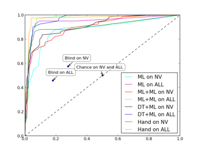
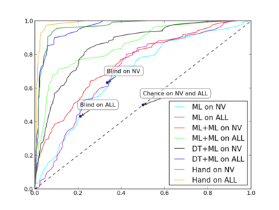
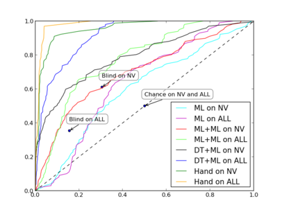
Figure 1: ROC curves for size ratios of (a) 0.67, (b) 0.33, and (c) 0.17.

Several observations can be made from the figure. First, the performance of both DT and ML gradually increases as the ratio increases. Their performance is far from that of hand on the smallest training set with ratio 0.17 while it is very close on the largest training set with ratio 0.67. This implies that as the learning problem is better constrained given more training data, both training algorithms find better local maxima. Second, the performance gap between DT and ML gradually decreases as the ratio increases. With ratio 0.17, although both DT and ML perform poorly, the gap between them is the largest. In this case, the learning problem is highly unconstrained, which makes ML suffer more severely from incorrect local optima than DT. However, with ratio 0.67, the problem is well constrained and there is almost no performance gap; sometimes ML performs even better than DT. Third, the two-phase ml+ml performs generally better than the one-phase ml. Fourth, results on ALL are generally better than those on NV. The reason is that longer sentences with varied parts of speech incorporate more information into the scoring function from Eq. 5.

6 Conclusion

We have proposed a DT framework for learning word meaning representations from video clips paired with only sentential labels in a weakly supervised fashion. Our method is able to automatically determine the word-to-meaning mappings from the sentences to the video data. Unlike the ML framework, our framework exploits not only the information of positive sentential labels but also that of negative labels, which makes the learning problem better constrained given the same amount of video data. We have demonstrated that DT significantly outperforms ML on small training datasets. Currently, the learning problem makes several assumptions about knowing: the grammar, the arity of each entry in the lexicon, and the participant number in each sentence, etc. In the future, we seek to gradually remove these assumptions by also learning these knowledge from training data.

Acknowledgments

This research was sponsored by the Army Research Laboratory and was accomplished under Cooperative Agreement Number W911NF-10-2-0060. The views and conclusions contained in this document are those of the authors and should not be interpreted as representing the official policies, either express or implied, of the Army Research Laboratory or the U.S. Government. The U.S. Government is authorized to reproduce and distribute reprints for Government purposes, notwithstanding any copyright notation herein.

References

- Bahl et al. (1986) L. Bahl, P. Brown, P. De Souza, and R. Mercer. Maximum mutual information estimation of hidden Markov model parameters for speech recognition. In Proceedings of the IEEE International Conference on Acoustics, Speech, and Signal Processing, volume 11, pages 49–52, 1986.
- Barbu et al. (2012a) A. Barbu, A. Bridge, Z. Burchill, D. Coroian, S. Dickinson, S. Fidler, A. Michaux, S. Mussman, N. Siddharth, D. Salvi, L. Schmidt, J. Shangguan, J. M. Siskind, J. Waggoner, S. Wang, J. Wei, Y. Yin, and Z. Zhang. Video in sentences out. In Proceedings of the Twenty-Eighth Conference on Uncertainty in Artificial Intelligence, pages 102–112, 2012a.
- Barbu et al. (2012b) A. Barbu, N. Siddharth, A. Michaux, and J. M. Siskind. Simultaneous object detection, tracking, and event recognition. Advances in Cognitive Systems, 2:203–220, Dec. 2012b.
- Baum (1972) L. E. Baum. An inequality and associated maximization technique in statistical estimation of probabilistic functions of a Markov process. Inequalities, 3:1–8, 1972.
- Baum and Petrie (1966) L. E. Baum and T. Petrie. Statistical inference for probabilistic functions of finite state Markov chains. The Annals of Mathematical Statistics, 37(6):1554–1563, 1966.
- Baum et al. (1970) L. E. Baum, T. Petrie, G. Soules, and N. Weiss. A maximization technique occuring in the statistical analysis of probabilistic functions of Markov chains. The Annals of Mathematical Statistics, 41(1):164–171, 1970.
- Felzenszwalb et al. (2010a) P. F. Felzenszwalb, R. B. Girshick, D. McAllester, and D. Ramanan. Object detection with discriminatively trained part-based models. IEEE Transactions on Pattern Analysis and Machine Intelligence, 32(9):1627–1645, Sept. 2010a.
- Felzenszwalb et al. (2010b) P. F. Felzenszwalb, R. B. Girshick, and D. A. McAllester. Cascade object detection with deformable part models. In Proceedings of the IEEE Conference on Computer Vision and Pattern Recognition, pages 2241–2248, 2010b.
- Gopalakrishnan et al. (1991) P. S. Gopalakrishnan, D. Kanevsky, A. Nadas, and D. Nahamoo. An inequality for rational functions with applications to some statistical estimation problems. IEEE Transactions on Information Theory, 37(1):107–113, Jan. 1991.
- He et al. (2008) X. He, L. Deng, and W. Chou. Discriminative learning in sequential pattern recognition. IEEE Signal Processing Magazine, 25(5):14–36, Sept. 2008.
- Jiang (2010) H. Jiang. Discriminative training of HMMs for automatic speech recognition: A survey. Computer Speech and Language, 24(4):589–608, Oct. 2010.
- Khan and Gotoh (2012) M. U. G. Khan and Y. Gotoh. Describing video contents in natural language. In Proceedings of the Workshop on Innovative Hybrid Approaches to the Processing of Textual Data, pages 27–35, 2012.
- Kojima et al. (2002) A. Kojima, T. Tamura, and K. Fukunaga. Natural language description of human activities from video images based on concept hierarchy of actions. International Journal of Computer Vision, 50(2):171–184, Nov. 2002.
- Krishnamoorthy et al. (2013) N. Krishnamoorthy, G. Malkarnenkar, R. J. Mooney, K. Saenko, and S. Guadarrama. Generating natural-language video descriptions using text-mined knowledge. In Proceedings of the 27th AAAI Conference on Artificial Intelligence, 2013.
- Kulkarni et al. (2011) G. Kulkarni, V. Premraj, S. Dhar, S. Li, Y. Choi, A. C. Berg, and T. L. Berg. Baby talk: Understanding and generating simple image descriptions. In Proceedings of the IEEE Conference on Computer Vision and Pattern Recognition, pages 1601–1608, 2011.
- Kuznetsova et al. (2012) P. Kuznetsova, V. Ordonez, A. C. Berg, T. L. Berg, and Y. Choi. Collective generation of natural image descriptions. In Proceedings of the 50th Annual Meeting of the Association for Computational Linguistics, pages 359–368, 2012.
- Lee et al. (2008) M. W. Lee, A. Hakeem, N. Haering, and S.-C. Zhu. SAVE: A framework for semantic annotation of visual events. In IEEE Computer Society Conference on Computer Vision and Pattern Recognition Workshops, pages 1–8, 2008.
- Ordonez et al. (2011) V. Ordonez, G. Kulkarni, and T. L. Berg. Im2text: Describing images using 1 million captioned photographs. In Advances in Neural Information Processing Systems, pages 1143–1151, 2011.
- Siskind (1996) J. M. Siskind. A computational study of cross-situational techniques for learning word-to-meaning mappings. Cognition, 61(1-2):39–91, Oct. 1996.
- Viterbi (1967) A. J. Viterbi. Error bounds for convolutional codes and an asymtotically optimum decoding algorithm. IEEE Transactions on Information Theory, 13(2):260–267, Apr. 1967.
- Walther and Griewank (2012) A. Walther and A. Griewank. Getting started with ADOL-C. In Combinatorial Scientific Computing, chapter 7, pages 181–202. Chapman-Hall CRC Computational Science, 2012.
- Wengert (1964) R. E. Wengert. A simple automatic derivative evaluation program. Commun. ACM, 7(8):463–464, 1964.
- Yao et al. (2010) B. Z. Yao, X. Yang, L. Lin, M. W. Lee, and S.-C. Zhu. I2T: Image parsing to text description. Proceedings of the IEEE, 98(8):1485–1508, Aug. 2010.
- Yu and Siskind (2013) H. Yu and J. M. Siskind. Grounded language learning from video described with sentences. In Proceedings of the 51st Annual Meeting of the Association for Computational Linguistics, 2013.