Factorising equity returns in an emerging market through exogenous shocks and capital flows

Abstract

A technique from stochastic portfolio theory [Fernholz, 1998] is applied to analyse equity returns of Small, Mid and Large cap portfolios in an emerging market through periods of growth and regional crises, up to the onset of the global financial crisis. In particular, we factorize portfolios in the South African market in terms of distribution of capital, change of stock ranks in portfolios, and the effect due to dividends for the period Nov 1994 to May 2007. We discuss the results in the context of broader economic thinking to consider capital flows as risk factors, turning around more established approaches which use macroeconomic and socio-economic conditions to explain Foreign Direct Investment (into the economy) and Net Portfolio Investment (into equity and bond markets).

1 Introduction

Risk factors driving equity portfolio returns may include performance measurements relative to some market index as in the capital asset pricing model (CAPM [16, 22, 19, 24] and its offspring) or more general arbitrage pricing theory (APT, [21]) risk factors in neo-classical finance. Some portfolio managers may select securities based on performance variables such as earnings-per-share or price-to-book estimates while others may be interested in valuations which are explained in terms of macroeconomic factors such as interest rates, inflation, GDP, market index or forex levels. The size effect refers to empirical evidence that small-capitalised stocks exhibit higher long-term performance than larger capitalised stocks [3]. This led to the development the Fama and French model to explain market, size and value ([2, 4]) components of equity returns by means of three APT-consistent risk factors [8].

Historically a simple motivation for the size effect is that some concerns with small capitalisation have potential for growth which may be far greater than any large cap stock. According to contemporary classifications in the US market, stocks may be classified in the following size-based scheme:

Mega cap	200 billion USD and greater
Big cap	10 billion USD and greater
Mid cap	2-10 billion USD
Small cap	300 million - 2 billion USD
Micro cap	50-300 million USD
Nano cap	under 50 million USD

According to the global classification, in 2013 the top 14 stock on the JSE are Big caps with the next 2 on the Big-Mid boundary. The largest 70 JSE stocks are global Mid caps, while the remaining top 100 are all worth more than 1 billion USD, placing them within global Small cap range.

Capitalisation of stocks in the SA equity market peaked at 833,548 million USD in 2007, dropped in 2008 and rose to 1,012,540 million USD by 2010 before dropping back to 2007 levels in 2011. This volatile behaviour has obviously been driven by the global financial crisis (GFC). Small cap indices show exacerbated fragility through the GFC, where values more than tripled before collapsing to 1998 levels by the end of 2008. Figure  1 plots the course of the MSCI Emerging Markets Small Cap Index, “which includes small cap representation across 21 Emerging Markets countries”, with 1,775 constituents. This index “tracks roughly 14% of the (free float-adjusted) market capitalization in each country.” Clearly oscillations in cross-border portfolio flows have nontrivial effects on conditions in a developing market (see also [17]) and a better understanding of small cap stocks is relevant for investments of various horizons particularly during periods of quantitative easing and withdrawal thereof [7].

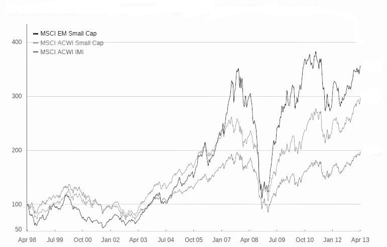
Figure 1: At the peak of equity markets in 2007, the MSCI index for Emerging Market (EM) Small Cap outperforms the All Country World Index (ACWI) Small Cap which in turn outperforms the ACWI Investable Market Index (IMI) before all collapse to ’98/’99 levels in 2008. The graphs depict cumulative index performance based on net returns.

Underlying reasons for the size-effect continue to be debateable. One plausible explanation came from the so-called stochastic portfolio theory (SPT) of Fernholz [10]. In [15] we reviewed the SPT rank-based construction and showed outperformance of small cap portfolios can be obtained in purely Gaussian price formation models. Under a simplifying assumption (discussed in Section  3.1), it is easy to generate a nullcase in which the selection mechanism, and not some meaningful performance related attribute, can explain outperformance in a random price market. This suggests that arguments which attribute size to being a proxy for some risk premium such as liquidity or capacity for firm-related growth in the economy are only part of the story.

When the model was proposed for US equity markets in 1999, Fernholz was interested in isolating a size factor[11, 12]. In that research, the effect was isolated in a market which, by 1999, had seen significant capital growth just before the violent swings since the dotcom bubble. In [13] 60yrs of data, 1939-1999, are examined to isolate a size effect. Fernholz’s empirical analysis of so-called distributional components covered the period 1989-1999 [13]. The period 1989-1999 is also used to examine components of returns in a portfolio generated via ranking in value. In that analysis, the distributional component is noted to be correlated to an entropy-based measure of diversity. The findings were similar in the paper [11] for the period 1975-1999.

We claim that SPT is particularly useful as a lens in emerging markets to separate market capital distribution from investor preferences based on ranking. In particular, the distributional, rank and dividend components of a SPT factorisation offer useful maps to capital flow, size (by market cap or other rank-based investment criteria) and profit taking factors to explain equity prices. This suggests a novel perspective toward unravelling the nature of portfolio flows as a risk factor in financial markets.

While there are investigations to uncover the economic factors which drive cross-border cashflows [20] complemented by critical discussion thereof [1, 18], to our knowledge there is very little empirical work which considers the effect of net portfolio investment (NPI) as a macroeconomic factor driving growth in a market sector. In [14], the relationship between weekly equity returns for JSE listed stock between Jan 2002 and Dec 2006 and NPI is investigated. A (linear) vector autoregressive model is used to identify lead and lag effects between these factors. In that work evidence is found that returns on the JSE tend to forecast NPI and find an absence of an impact of NPI on returns.

In this paper we document the SPT decomposition of portfolios constructed via size and value criteria. We also observe that significant changes in components are indicative of changes of states which, as expected, appear to be correlated to changes in levels of cross-border portfolios flows and investment. In our investigation we focus on price formation in the South African (SA) equity market for the period Nov 1994 to May 2007. In this post-democracy to pre-GFC period, SA market pricing has been impacted by numerous exogenous events including three ZAR currency crises, the Asian crisis of 1997, the dotcom bubble, the USA 9/11 Twin Trade tower collapses in 2001, the 2nd Iraq war and the resources and property booms up to 2007. Taking into account tacit market knowledge about features such as liquidity and bid-offer spreads for specific stocks between 1994 and 2007, we construct Small, Mid and Large cap portfolios by setting thresholds in the ranked market caps. We also use book-value-to-price information to construct a Value portfolio for complementary analysis. Our investigation exposes correlations between regime changes in investment trends in JSE equities and NPI. This is in keeping with post GFC developments to better address the failures of orthodox economic theory and to better account for imperfect knowledge [5, 23].

2 Continuous time stochastic rank-based
capital distribution

We recap some notation and key results for describing the main decomposition [12, 13].

2.1 Growth rates and rates of return

The continuous time formulation of the SPT framework makes it compatible with other continuous time models used in pricing securities. Generalisation of the simpler discrete time analysis depends on applications of It$\hat{o}$’s lemma and a representation of rank crossovers in terms Tanaka’s formula for Brownian local times.

The use of market capitalisation (cap) instead of price in the SPT modelling framework facilitates measurement of capital distribution through the market. For the purpose of this discussion we assume a market without corporate events such as mergers and acquisitions, spinoffs, etc. The construction of size-based portfolios then becomes a easy exercise in ranking stocks from biggest to smallest cap and determining a threshold to separate large from small. The continuous time formulation is able to quantify activity at the boundary through (stochastic) local time measurement of multivariate processes.

A stock is modelled by its market cap, where the total value of shares issued by the $i^{th}$ corporation is denoted $X_{i}$. We sometimes refer to this as the stock price, a shareholder may hold a fraction of this share and prices are assumed to be driven by an idiosyncratic drift coupled to a market multivariate Wiener noise process: [10]:

$$d\log X_{i}(t)= \underbrace{\gamma_{i}(t)dt} +\sum\limits_{\nu=1}^{n}\xi_{i\nu}(t)dW_{\nu}(t)\hskip 99.58464pt$$

growth rate

where $(W_{1},...,W_{n})$ is standard Brownian motion, $\gamma_{i}$ is measurable, adapted and for all $T>0$, $i=1,...n$, satisfies the condition $\int_{0}^{T}|\gamma_{i}(t)|dt<\infty$ a.s., the $\xi_{i\nu}$, $\nu=1,...n$ are measurable, adapted and satisfy $\int_{0}^{T}\sum\limits_{\nu=1}^{n}\xi_{i\nu}^{2}(t)dt<\infty$ for all $T>0$, a.s. and $\lim\limits_{t\rightarrow\infty}\frac{1}{t}\sum\limits_{\nu=1}^{n}\xi_{i\nu}^{2}(t)\log\log t=0$. The processes $\gamma_{i}$ and $\xi_{i\nu}$ represent the growth rate and the volatility of the $i^{th}$ stock, respectively.

An application of It$\hat{o}$’s lemma leads to

$$dX_{i}(t)= \underbrace{\left(\gamma_{i}(t)+\frac{1}{2}\sum\limits_{\nu=1}^{n}\xi_{i\nu}^{2}(t)\right)} X_{i}(t)dt+X_{i}(t)\sum\limits_{\nu=1}^{n}\xi_{i\nu}(t)dW_{\nu}(t),$$

rate of return

where $\alpha(t)=\gamma_{i}(t)+\frac{1}{2}\sum\limits_{\nu=1}^{n}\xi_{i\nu}^{2}(t)$ is referred to as the rate of return process.

According to Fernholz, while the rate of return is used in classical portfolio theory, the growth rate is a better indicator of long-term behaviour. As a special case, it is notable that if growth rates are assumed to be constant, then long-term equilibrium will exist only if growth rates are the same for all stocks in the market. If any stock were to have a higher growth rate relative to the rest, then that stock would eventually dominate the market and stocks with lower growth rates would disappear. In reality, growth rates are not constant and markets are more likely to be impacted by global events outside the model.

2.2 Portfolios and portfolio growth rates

The market is viewed as the family of all stocks $X_{1},\ldots,X_{n}$, where two stocks are equivalent if they differ by at most a constant. A portfolio $\pi$ is defined to be a positive-valued combination of stocks such that

$$Z_{\pi}=\pi_{1}Z_{\pi}+\ldots\pi_{n}Z_{\pi},$$ (3)

where the $\pi_{i}$ are functions of time and denote the proportion of $Z_{\pi}$ invested in $X_{i}$. The quantity $\pi_{i}Z_{\pi}$ is the amount invested in $X_{i}$ and thus, a portfolio $\pi$ can represented by the weights allocated to each stock, $\pi_{1},\ldots,\pi_{n}$, at time $t$. It is assumed that these weights are bounded and sum to unity, $\sum\pi_{i}=1$, so that the portfolio is fully invested in stocks.

It is also useful to differentiate between a passive portfolio, where the fractional number of shares held in each stock are constants: $Z_{\nu}=\nu_{1}X_{1}+\ldots\nu_{2}X_{2}$, and a balanced portfolio where the proportions $\pi_{i}$ are constant. The proportions can be related to the fractional number of units held as $\pi_{i}=\nu_{i}X_{i}/Z_{\nu}$. Here constant values for $\nu_{i}^{\prime}s$ imply that the proportions $\pi_{i}$ are not necessarily constant.

• (Market Portfolio) The market portfolio $\mu$ has weights $\mu_{1},\ldots,\mu_{n}$ given by:

  $$\mu_{i}(t)=\frac{X_{i}(t)}{X_{1}(t)+\ldots+X_{n}(t)},$$ (4)

  for $t\in[0,T]$, $i=1,\ldots,n$; the weights $\mu_{i}(t)$ are called the market weights.

The value of the market portfolio,

$$Z_{\mu}(t)=X_{1}(t)+\ldots+X_{n}(t),$$ (5)

is the combined capitalisation of all the stocks in the market at a given time.

From the definitions of the price processes of stocks, it follows that

$$d\log Z_{\pi}(t)= \gamma_{\pi}(t)dt+\sum\limits_{i,\nu}\pi_{i}(t)\xi_{i\nu}dW_{\nu}(t),\hskip 128.0374pt$$ (6)

$$\textrm{ where}\hskip 14.22636pt\gamma_{\pi}(t)= \underbrace{\sum_{i}\pi_{i}(t)\gamma_{i}(t)+\frac{1}{2}\left(\sum_{i}\pi_{i}(t)\sigma_{ii}(t)-\sum_{i,j}\pi_{i}(t)\pi_{j}(t)\sigma_{ij}(t)\right)}$$

portfolio growth rate

$$\textrm{and}\hskip 14.22636pt\sigma_{ij}(t)= \sum_{\nu}\xi_{i\nu}(t)\xi_{j\nu}(t)dt.\hskip 184.9429pt$$

Equivalently,

$$d\log Z_{\pi}(t) = \sum_{i}\pi_{i}(t)\gamma_{i}(t)dt+\gamma_{\pi}^{*}(t)dt+\sum\limits_{i,\nu}\pi_{i}(t)\xi_{i\nu}dW_{\nu}(t),$$ (7)

$$\textrm{ where}\hskip 14.22636pt\gamma^{*}_{\pi}(t) = \underbrace{\frac{1}{2}\left(\sum_{i}\pi_{i}(t)\sigma_{ii}(t)-\sum_{i,j}\pi_{i}(t)\pi_{j}(t)\sigma_{ij}(t)\right)}.$$ (8)

excess growth rate

The portfolio growth rate exceeds the weighted average of the individual growth rates by the amount referred to as the excess growth rate. The logarithmic representation exposes this insight. In the standard representation, the portfolio rate of return is simply the portfolio weighted sum of the rates of returns of the stocks comprising it.

Given a portfolio $\pi$, one may consider its performance relative to the market:

$$d\log(Z_{\pi}(t)/Z_{\mu}(t))=\sum_{i}\pi_{i}(t)d\log\mu_{i}(t)+\gamma_{\pi}^{*}(t)dt.$$ (9)

In particular, it is possible to understand the relative returns in terms of changes in the market weights and the excess growth rate process [13].

2.3 Functionally generated portfolios

Motivated by the relative performance of an entropy weighted portfolio, Fernholz introduced the notion of a functionally generated portfolio. In this approach, relative performance of a portfolio can be decomposed into two distinct components within a stochastic differential equation. The first component is the logarithmic change in the value of the generating function, the second term involves the relative covariances of the stocks in the portfolio.

A portfolio is constructed based on the entropy function:

$$\mathbf{S}(x)=-\sum_{i=1}^{n}x_{i}\log x_{i}$$

for all $x\in\Delta^{n}=\{x\in\mathbf{R}^{n}|\sum x_{i}=1,x_{i}>0\}$. The market entropy process is defined by

$$\mathbf{S}(\mu(t))=-\sum_{i=1}^{n}\mu_{i}(t)\log\mu_{i}(t),\ \ t\in[0,T],$$ (10)

where $\mu$ denotes the market portfolio and the portfolio $\pi$ with weights

$$\pi_{i}(t)=\frac{\mu_{i}(t)\log\mu_{i}(t)}{\mathbf{S}(\mu(t))},\ \ t\in[0,T],i=1...n,$$ (11)

is called the entropy weighted portfolio. It can be shown that

$$d\log\mathbf{S}(\mu(t))=d\log\left(\frac{Z_{\pi}(t)}{Z_{\mu}(t)}\right)-\frac{\gamma^{*}_{\mu}(t)}{\mathbf{S}(\mu(t))}.$$ (12)

Generalising this construction is the idea of a functionally generated portfolio, which provides a decomposition of the relative rate of return of portfolio weights into two distinct components within a stochastic differential equation.

• (Generating functions and functionally generated portfolios) Let $\mathbf{S}$ be a positive continuous function defined on $\Delta^{n}$, and let $\pi$ be a portfolio. $\mathbf{S}$ is said to generate $\pi$ if there exists a measurable process of bounded variation $\Theta$ such that for all $t\in[0,T]$, a.s.

  $$\log(Z_{\pi}/Z_{\mu})=\log\mathbf{S}(\mu(t))+\Theta(t),$$ (13)

  The process $\Theta$ is called the drift process corresponding to $\mathbf{S}$ If $\mathbf{S}$ generates $\pi$, then $\mathbf{S}$ is called the generating function of $\pi$, and $\pi$ is said to be functionally generated.

Equation (13) can be expressed in differential form as

$$d\log(Z_{\pi}(t)/Z_{\mu}(t))=d\log\mathrm{S}(\mu(t))+d\Theta(t),$$ (14)

a.s., for all $t\in[0,T]$. It is this differential form that is typically used.

2.4 Rank processes

To investigate the size effect, one may consider a portfolio generating function based on a market cap rank process. Making the notion of rank mathematically precise, one may define the $k$th ranked number of the set $\{x_{1},...,x_{n}\}\subset\mathbb{R}$ to be

$$x_{(k)}=\max\limits_{1\leq i_{1}<...<i_{k}\leq n}\min(x_{i_{1}},...x_{i_{k}}),\ \ \ 1\leq k\leq n.$$ (15)

It follows that

$$x_{(1)}\geq x_{(2)}\geq...\geq x_{(n)}.$$ (16)

If $X_{1},...,X_{n}$ are stochastic processes, then the $k$th ranked process at time $t\in[0,T]$ of $\{X_{1},....X_{n}\}$ is defined to be

$$X_{(k)}(t)=\max\limits_{1\leq i_{1}<...<i_{k}\leq n}\min(X_{i_{1}}(t),...,X_{i_{k}}(t)),\ \ \ 1\leq k\leq n$$ (17)

To obtain mathematical expressions for the time-varying portfolio $\pi$ and drift process $\Theta$ for a generating functions based on rank processes, one needs to appeal to local times of semi-martingales. These describe the occupation time that a process spends at a specific level. In the context at hand it is used to quantify transitions between large cap and small cap portfolios. Specifically, local times of rank differences at the boundary are instantaneously zero when there is a rank crossover.

For the continuous semi-martingale $M$ in the next theorem, the local time process counts the number of times that $M$ hits zero..

Theorem 2.1.

(Tanaka’s formula for local times) Let $M$ be a continuous semi-martingale. Then the local time (at 0) for $M$ is the process $\Lambda_{M}$ defined for $t\in[0,T]$ by

$$\Lambda_{M(t)}=\frac{1}{2}\left({|M(t)|-|M(0)|-\int_{0}^{t}\textrm{sgn}(M(s))dM(s)}\right),$$ (18)

where $\textrm{sgn}(m)=2I_{(0,\infty)}(m)-1$, with $I_{(0,\infty)}$ the indicator function of $(0,\infty)$.

Considering Equation ( 18) in differential form and using the equivalences $\max(X,Y)=\frac{X+Y}{2}+\frac{|X-Y|}{2}$ and $\min(X,Y)=-\max(-X,-Y)$, it can be shown that rank processes derived from pathwise mutually non-degenerate absolutely continuous semi-martingales can be expressed in terms of the original process adjusted by local times. As a corollary, one obtains the following result for market weight processes:

Proposition 2.2.

Consider a market of stocks $X_{1},\ldots,X_{n}$ which are pathwise mutually non-degenerate. The market weight processes $\mu_{1},...,\mu_{n}$, satisfy

$$d\log\mu_{p_{t}(k)}(t) =\sum_{i=1}^{n}I_{\{i\}}(p_{t}(k))d\log\mu_{i}(t)$$ (19)

$$+ \frac{1}{2}\left({d\Lambda_{\log\mu_{p_{t}(k)}-\log\mu_{p_{t}(k+1)}}(t)-d\Lambda_{\log\mu_{p_{t}(k-1)}-\log\mu_{p_{t}(k)}}(t)}\right).$$ (20)

a.s, for $t\in[0,T]$, where $p_{t}$ is the random permutation of $\{1,\ldots,n\}$, such that for $k=1,\ldots,n$.

$$\mu_{p_{t}(k)}(t) = \mu_{(k)}(t),$$ (21)

$$~{}\mathrm{if}~{}\mu_{p_{t}(k)}(t) = \mu_{p_{t}(k+1)}(t),~{}\mathrm{then}~{}p_{t}(k)<p_{t}(k+1)$$ (22)

Proposition  2.2 is applied to obtain the following key result which determines the portfolio weights $\pi$ and drift $\Theta$ for a portfolio generating function which models an evolution of ranks through time.

Theorem 2.3.

(Rank process generated portfolios) Let ${\cal M}$ be a market of stock $X_{1},\ldots,X_{n}$ that are pathwise mutually non-degenerate, let $p_{t}$ be the random permutation defined as in Proposition 2.2. Let ${\mathbf{S}}$ be a function defined on a neighborhood $U$ of $\Delta_{n}$. Suppose that there exits a positive $S\in C^{2}(U)$ such that for $(x_{1},\ldots,x_{n})\in U$, $\mathbf{S}(x_{1},\ldots,x_{n})=S(x_{p_{t}(1)},\ldots,x_{p_{t}(n)})$, and for $i=1,\ldots,n$, and $x_{i}D_{i}\log S(x)$ bounded for $x\in\Delta^{n}$. Then $\mathbf{S}(x)$ generates the portfolio $\pi$ such that for $k=1,\ldots,n$,

$$\pi_{p_{t}(k)}(t)=\left({D_{k}\log S(\mu_{p_{t}}(t))}+1-\sum_{j=1}^{n}{\mu_{p_{t}(j)}D_{j}\log S(\mu_{p_{t}}(t))}\right)\mu_{p_{t}(k)}(t),$$ (23)

for all $t\in[0,T]$, a.s., with a drift process $\Theta$.

$$d\Theta(t)=\theta_{\pi}(t)dt+dL_{\pi}(t),$$ (24)

for all $t\in[0,T]$, a.s. where, a.s.,

$$\theta_{\pi}(t)={-1\over 2\mathbf{S}(\mu(t))}\sum_{i,j=1}^{n}D_{ij}S(\mu_{p_{t}}(t))\mu_{p_{t}(i)}(t)\mu_{p_{t}(j)}(t)\tau_{p_{t}(ij)}(t)dt$$ (25)

for $t\in[0,T]$, and

$$dL_{\pi}(t)=\frac{1}{2}\sum_{k=1}^{n-1}\left({\pi_{p_{t}(k+1)}(t)-\pi_{p_{t}(k)}(t)}\right)d\Lambda_{\log\mu_{p_{t}(k)}-\log\mu_{p_{t}(k+1)}}(t)$$ (26)

and for $t\in[0,T]$, $\tau_{ij}(t)=\sigma_{ij}(t)-\sigma_{i\mu}(t)-\sigma_{j\mu}(t)+\sigma_{\mu\mu}(t),$ $\sigma_{i\mu}(t)=\sum\limits_{j=1}^{n}\mu_{j}(t)\sigma_{ij}(t)$ and $\sigma_{\mu\mu}(t)=\mu(t)\sigma(t)\mu^{T}(t)$.

The relative rank covariance process is denoted $\tau_{p_{t}(ij)}=\tau_{p_{t}(i)p_{t}(j)}(t)$ for $i,j=1,\ldots n$ and the ranked market weights $\mu_{p_{t}(1)},\ldots,\mu_{p_{t}(n)}$ generate $\mu_{p_{t}}=(\mu_{p_{t}(1)},\ldots,\mu_{p_{t}(n)})$. The first term of the drift, $\theta_{\pi}(t)dt$ is the smooth component and the second term, $dL_{\pi}$ is the local time component.

2.5 Size in continuous time

We review the construction of portfolio generating functions that partition the market into mutually exclusive portfolios of large capitalisation and small capitalisation stock.

Let $1<m<n$ and consider the generating function for the large portfolio:

$$\mathbf{S}_{L}(x)=x_{p_{t}(1)}+\ldots+x_{p_{t}(m)}.$$ (27)

This represents the relative capitalisation of a large-stock index composed of the $m$ largest stocks in the market. By Theorem 2.3, $\mathbf{S}_{L}$ generates a portfolio $\xi$ with weights given by:

$$\xi_{p_{t}(k)}(t)=\left\{{\begin{array}[]{ll}{\mu_{p_{t}(k)}(t)\over\mathbf{S}(\mu(t))},&k\leq m\\ 0,&k>m\end{array}}\right.$$ (30)

for $t\in[0,T]$, where weights $\xi_{i}$ for $i=1,\ldots,m$ represent the capitalisation weights of the stocks in the large stock index.

Hence, the function $\mathbf{S}_{L}$ generates a large portfolio with returns relative to the market portfolio given by:

$$d\log(Z_{\xi}(t)/Z_{\mu}(t))=d\log\mathrm{S}_{L}(\mu(t))-\frac{1}{2}\xi_{p_{t}(m)}(t)d\Lambda_{\log\mu_{p_{t}(m)}-\log\mu_{p_{t}(m+1)}}(t),$$ (31)

for all $t\in[0,T]$, a.s. Here all but the last local time term drops out.

The generating function for the corresponding small portfolio is given by:

$$\mathbf{S}_{S}(x)=x_{p_{t}(m+1)}+\ldots+x_{p_{t}(n)},$$ (32)

with

$$d\log(Z_{\eta}(t)/Z_{\mu}(t))=d\log\mathrm{S}_{S}(\mu(t))+\frac{1}{2}\eta_{p_{t}(m+1)}(t)d\Lambda_{\log\mu_{p_{t}(m)}-\log\mu_{p_{t}(m+1)}}(t),$$ (33)

for $t\in[0,T]$. Here $\mathbf{S}_{S}(x)$ represents the relative capitalisation of a small stock index comprised of the $n-m$ smallest stocks in the market.

Combining Equations (31) and (33) we obtain the relative return of the small to large portfolios:

$$d\log\left({Z_{\eta}(t)\over Z_{\xi}(t)}\right) = d\log\left({\mathrm{S}_{S}(\mu(t))\over\mathrm{S}_{L}(\mu(t))}\right)$$ (35)

$$+\frac{1}{2}\left({\xi_{p_{t}(m)}(t)+\eta_{p_{t}(m+1)}(t)}\right)d\Lambda_{\log\mu_{p_{t}(m)}-\log\mu_{p_{t}(m+1)}}$$

Fernholz observed that if the relative capitalisation of the small to large portfolio does not change significantly, then the first term, dependent on $\mathbf{S}_{S}\over\mathrm{S}_{L}$, does not change by much either. This implies that the relative returns are dependent on the local time terms.

3 Model-free discrete factorization of single
stock returns in a ranked market

Throughout this section we consider a discrete time market, with the $i^{th}$ stock modelled by it’s market capitalisation $X_{i}(t)$ at time $t$ and the total market cap denoted by $M(t)=\sum\limits_{i=1}^{N}X_{i}(t)$. No assumptions are required for the evolution of prices. It suffices that stocks can be ranked by capitalisation to obtain the factorisation given in Equation ( 37) for the case of no-dividends and Equation ( 39) for a market with dividend paying stocks  [11].

At each time step and the weight of the $i^{th}$ ranked stock is denoted as before as $\mu_{i}(t)={X_{i}(t)\over M(t)}.$ In particular, we assume that these market weights are conveniently indexed in descending order according to size at time $t$. Each time iteration brings price changes and possible rank changes. Notationally this is captured by letting $\mu_{p_{t}(i)}(t)$ denote the weight of the $i^{th}$ ranked stock at time $t$. The map $p_{t}$ denotes a permutation which operates on weights of ranked stocks and the subscript of $\mu$ points to the rank at the time of measurement:

$$\{\mu_{1}(t_{0}),\ldots,\mu_{n}(t_{0})\}\stackrel{{\scriptstyle p_{t}}}{{\longrightarrow}}\left\{\mu_{p_{t}(1)}(t),\ldots,\mu_{p_{t}(n)}(t)\right\}.$$ (36)

Assuming no dividends, after the iteration from time $t_{0}$ to time $t$, the weight of the stock in rank $i$ at time $t_{0}$, $\mu_{i}(t_{0})$, gets mapped to the weight of the stock in rank $i$ at time $t_{1}$, $\mu_{p_{t_{1}}(i)}(t_{1})$. This is referred to as the distribution component of the transformation. Meanwhile, the stock which was at rank $i$ at time $t_{0}$ may occupy a new ranking at time $t_{1}$, which we can denote $\mu_{p_{t_{0}}(i)}(t_{1})$. The mapping from old rank to new of a specific stock is referred to as the time component. This can be graphically represented (as in [11]).

$$\lx@xy@svg{\hbox{\raise 0.0pt\hbox{\kern 18.87614pt\hbox{\ignorespaces\ignorespaces\ignorespaces\hbox{\vtop{\kern 0.0pt\offinterlineskip\halign{\entry@#!@&&\entry@@#!@\cr&&\\&&\crcr}}}\ignorespaces{\hbox{\kern-18.87614pt\raise 0.0pt\hbox{\hbox{\kern 0.0pt\raise 0.0pt\hbox{\hbox{\kern 3.0pt\raise 0.0pt\hbox{$\textstyle{\mu_{p_{t_{0}}(i)}(t_{0})\ignorespaces\ignorespaces\ignorespaces\ignorespaces\ignorespaces\ignorespaces\ignorespaces\ignorespaces}$}}}}}}}\ignorespaces\ignorespaces\ignorespaces{}\ignorespaces\ignorespaces{\hbox{\lx@xy@drawline@}}\ignorespaces\ignorespaces\ignorespaces{\hbox{\kern 29.46873pt\raise-15.55171pt\hbox{{}\hbox{\kern 0.0pt\raise 0.0pt\hbox{\hbox{\kern 3.0pt\hbox{\hbox{\kern 0.0pt\raise-2.15279pt\hbox{$\scriptstyle{t}$}}}\kern 3.0pt}}}}}}\ignorespaces{\hbox{\kern 46.10483pt\raise-30.909pt\hbox{\hbox{\kern 0.0pt\raise 0.0pt\hbox{\lx@xy@tip{1}\lx@xy@tip{-1}}}}}}\ignorespaces\ignorespaces{\hbox{\lx@xy@drawline@}}\ignorespaces{\hbox{\lx@xy@drawline@}}\ignorespaces\ignorespaces\ignorespaces\ignorespaces{}{\hbox{\lx@xy@droprule}}\ignorespaces\ignorespaces\ignorespaces{\hbox{\kern-9.6434pt\raise-20.7045pt\hbox{{}\hbox{\kern 0.0pt\raise 0.0pt\hbox{\hbox{\kern 3.0pt\hbox{\hbox{\kern 0.0pt\raise-2.43056pt\hbox{$\scriptstyle{d}$}}}\kern 3.0pt}}}}}}\ignorespaces{\hbox{\kern 0.0pt\raise-30.909pt\hbox{\hbox{\kern 0.0pt\raise 0.0pt\hbox{\lx@xy@tip{1}\lx@xy@tip{-1}}}}}}{\hbox{\lx@xy@droprule}}{\hbox{\lx@xy@droprule}}{\hbox{\kern 58.75229pt\raise 0.0pt\hbox{\hbox{\kern 0.0pt\raise 0.0pt\hbox{\hbox{\kern 3.0pt\raise 0.0pt\hbox{$\textstyle{}$}}}}}}}{\hbox{\kern 104.62843pt\raise 0.0pt\hbox{\hbox{\kern 0.0pt\raise 0.0pt\hbox{\hbox{\kern 3.0pt\raise 0.0pt\hbox{$\textstyle{}$}}}}}}}{\hbox{\kern-18.87614pt\raise-41.409pt\hbox{\hbox{\kern 0.0pt\raise 0.0pt\hbox{\hbox{\kern 3.0pt\raise 0.0pt\hbox{$\textstyle{\mu_{p_{t_{1}}(i)}(t_{1})\ignorespaces\ignorespaces\ignorespaces\ignorespaces}$}}}}}}}\ignorespaces\ignorespaces\ignorespaces\ignorespaces{}{\hbox{\lx@xy@droprule}}\ignorespaces\ignorespaces\ignorespaces{\hbox{\kern 26.19987pt\raise-45.91594pt\hbox{{}\hbox{\kern 0.0pt\raise 0.0pt\hbox{\hbox{\kern 3.0pt\hbox{\hbox{\kern 0.0pt\raise-1.50694pt\hbox{$\scriptstyle{r}$}}}\kern 3.0pt}}}}}}\ignorespaces{\hbox{\kern 42.87614pt\raise-41.409pt\hbox{\hbox{\kern 0.0pt\raise 0.0pt\hbox{\lx@xy@tip{1}\lx@xy@tip{-1}}}}}}{\hbox{\lx@xy@droprule}}{\hbox{\lx@xy@droprule}}{\hbox{\kern 42.87614pt\raise-41.409pt\hbox{\hbox{\kern 0.0pt\raise 0.0pt\hbox{\hbox{\kern 3.0pt\raise 0.0pt\hbox{$\textstyle{\mu_{p_{t_{0}}(i)}(t_{1})}$}}}}}}}{\hbox{\kern 104.62843pt\raise-41.409pt\hbox{\hbox{\kern 0.0pt\raise 0.0pt\hbox{\hbox{\kern 3.0pt\raise 0.0pt\hbox{$\textstyle{}$}}}}}}}\ignorespaces}}}}\ignorespaces, \textstyle{\mu_{p_{t_{0}}(i)}(t_{0})\ignorespaces\ignorespaces\ignorespaces\ignorespaces\ignorespaces\ignorespaces\ignorespaces\ignorespaces} \scriptstyle{t} \scriptstyle{d} \textstyle{\mu_{p_{t_{1}}(i)}(t_{1})\ignorespaces\ignorespaces\ignorespaces\ignorespaces} \scriptstyle{r} \textstyle{\mu_{p_{t_{0}}(i)}(t_{1})} \textstyle{\mu_{p_{t_{0}}(i)}(t_{0})\ignorespaces\ignorespaces\ignorespaces\ignorespaces\ignorespaces\ignorespaces\ignorespaces\ignorespaces} \scriptstyle{t} \scriptstyle{d} \textstyle{\mu_{p_{t_{1}}(i)}(t_{1})\ignorespaces\ignorespaces\ignorespaces\ignorespaces} \scriptstyle{r} \textstyle{\mu_{p_{t_{0}}(i)}(t_{1})}$$

The arrow labeled $d$ identifies the capital distribution part of the transformation, while the $t$ labels the time component. The diagram is completed with a transformation at time $t_{1}$ between ranks at that time, which we refer to as the rank component.

Now, still assuming no dividends, the log-return of the $i^{th}$ stock is:

$$\log\left(\frac{X_{i}(t_{1})}{X_{i}(t_{0})}\right),$$

with a return on the overall market portfolio for the same period computed as

$$\log\left(\frac{M(t_{1})}{M(t_{0})}\right).$$

Thus, computing returns relative to the market one obtains:

$$\log\left(\frac{X_{i}(t_{1})}{X_{i}(t_{0})}\right)-\log\left(\frac{M(t_{1})}{M(t_{0})}\right)=\log\left(\frac{\mu_{p_{t_{0}}(i)}(t_{1})}{\mu_{p_{t_{0}}(i)}(t_{0})}\right).$$

From the triangle factorisation above, one obtains:

$$\frac{\mu_{p_{t_{0}}(i)}(t_{1})}{\mu_{p_{t_{0}}(i)}(t_{0})}=\left(\frac{\mu_{p_{t_{1}}(i)}(t_{1})}{\mu_{p_{t_{0}}(i)}(t_{0})}\right)\left(\frac{\mu_{p_{t_{0}}(i)}(t_{1})}{\mu_{p_{t_{1}}(i)}(t_{1})}\right).$$ (37)

Taking logarithms in Equation ( 37), the right hand side is the sum of returns attributed to change in capital distribution plus a component due to change in rank:

$$\log\left({\mu_{p_{t_{0}}(i)}(t_{1})\over\mu_{p_{t_{0}}(i)}(t_{0})}\right)=\log\left({\mu_{p_{t_{1}}(i)}(t_{1})\over\mu_{p_{t_{0}}(i)}(t_{0})}\right)+\log\left({\mu_{p_{t_{0}}(i)}(t_{1})\over\mu_{p_{t_{1}}(i)}(t_{1})}\right)$$ (38)

Dividends may be incorporated as the return ${\delta_{p_{t_{0}}(i)}(t_{1})}$, measured in portfolio weight of the stock which was in rank $i$ at time $t_{0}$, with an additional branch to the factorisation:

Thus, we have the following summary of maps:

(Capital) Distribution component	$\mu_{p_{t_{0}}(i)}(t_{0})\longrightarrow_{d}\mu_{p_{t_{1}}(i)}(t_{1})$
Rank components	$\mu_{p_{t_{1}}(i)}(t_{1})\longrightarrow_{r}\mu_{p_{t_{0}}(i)}(t_{1})$
Time component	$\mu_{p_{t_{0}}(i)}(t_{0})\longrightarrow_{t}\mu_{p_{t_{0}}(i)}(t_{1})$
Dividend component	$\mu_{p_{t_{0}}(i)}(t_{1})\rightarrow_{\delta}\mu_{p_{t_{0}}(i)}(t_{1})e^{\delta_{p_{t}(i)}(t_{1})}$

The dividend rate for the market from ${t_{0}}$ to ${t_{1}}$ is given by:

$$\delta(t_{1})=\ln\left({\sum\mu_{p_{t_{0}}(i)}(t_{1})e^{\delta_{p_{t_{0}}(i)}(t_{1})}}\right),$$

where the dividend rate per stock for the time change between time ${t_{0}}$ and ${t_{1}}$ is denoted by $\delta_{p_{t_{0}}(i)}(t_{1}).$ Thus, the increase in value due to the dividend rate, at time ${t_{1}}$, is

$$\mu_{p_{t_{0}}(i)}(t_{1})e^{\delta_{p_{t_{0}}(i)}(t_{1})}$$

The dividend correction can, therefore, be computed as $(\delta(t_{1})+\delta_{p_{t_{0}}(i)}(t_{1}))$  and the return factorisation with dividends extends Equation ( 37) and is given by:

$$\log\left({\mu_{p_{t_{0}}(i)}(t_{1})\over\mu_{p_{t_{0}}(i)}(t_{0})}\right)=\log\left({\mu_{p_{t_{1}}(i)}(t_{1})\over\mu_{p_{t_{0}}(i)}(t_{0})}\right)+\log\left({\mu_{p_{t_{0}}(i)}(t_{1})\over\mu_{p_{t_{1}}(i)}(t_{1})}\right)+(\delta(t_{1})+\delta_{p_{t_{0}}(i)}(t_{1})).$$ (39)

3.1 Special-case proof of the size effect

The discrete time formulation is more simplistic but does not clearly discriminate between the contributions due to drift and changes in the relative capitalisation of stocks. However, it does afford some insight into how the mechanical construction is independent of the price process. Clearly if one has two mutually exclusive portfolios built on ranking stocks, there will cross-overs from the one portfolio to the other due to price volatility. In particular, outperformance can occur as statistical effect without in any way being risk premium

Consider a large cap portfolio, $Z_{L}$ of the biggest $m$ stocks and a small portfolio, $Z_{S}$, comprising the rest of the market:

$$Z_{L}(t_{0}) = X_{p_{t_{0}}(1)}(t_{0})+\ldots+X_{p_{t_{0}}(m)}(t_{0}),$$ (40)

$$Z_{S}(t_{0}) = X_{p_{t_{0}}(m+1)}(t_{0})+\ldots+X_{p_{t_{0}}(n)}(t_{0}).$$ (41)

At some later time $t_{1}$ the return for the $i$-th stock is $r_{i}(t_{0})=\log(X_{i}(t_{1})/X_{i}(t_{0}))$ so that the return of the large portfolio and small portfolio are

$$r_{L}(t_{1}) = \log(X_{p_{t_{0}}(1)}(t_{1})+\ldots+X_{p_{t_{0}}(m)}(t_{1})/Z_{L}(t_{0}))$$ (42)

$$r_{S}(t_{1}) = \log(X_{p_{t_{0}}(m+1)}(t_{1})+\ldots+X_{p_{t_{0}}(n)}(t_{1})/Z_{S}(t_{0})),$$ (43)

where the portfolio returns are computed before rebalancing according to new ranks. The portfolios are then reconstituted at time $t_{1}$. We now review the result that if the relative ratios remain constant then the return of the small portfolio is greater than the return of the large portfolio.

First observe that if the capitalisation ratios of the rebalanced portfolios do not change [11] then

$${Z_{L}(t_{1})\over Z_{L}(t_{0})}={Z_{S}(t_{1})\over Z_{S}(t_{0})}.$$ (44)

Now the large portfolio is comprised of the $m$ largest stocks at each time and hence:

$$Z_{L}(t_{1})\geq X_{p_{t_{0}}(1)}(t_{1})+\ldots+X_{p_{t_{0}}(m)}(t_{1})$$

with equality if and only if $\{p_{t_{1}}(1),\dots,p_{t_{1}}(m)\}=\{p_{t_{0}}(1),\dots,p_{t_{0}}(m)\}$.

Similarly $Z_{S}(t_{1})\leq X_{p_{t_{0}}(m+1)}(t_{1})+\ldots+X_{p_{t_{0}}(n)}(t_{1})$.

It follows from Equations (42) (43) respectively, that

$$r_{L}(t_{1}) \leq \log(Z_{L}(t_{1})/Z_{L}(t_{0}))$$ (45)

$$r_{S}(t_{1}) \geq \log(Z_{S}(t_{1})/Z_{S}(t_{0})).$$ (46)

Thus, by Equation (44), $r^{t_{1}}_{L}\leq r^{t_{1}}_{S}$.

Heuristically, the effect of rebalancing (in response to cross-overs in ranking) is that at each time companies performing worse (or that have had capitalisation reduced) get dropped into the small stock portfolio and stocks that have done well (or that have seen an increase in market capitalisation) in the small cap portfolio get bumped up. However, the computation of returns $r_{L}(t_{1})$ and $r_{S}(t_{1})$ is based on ranks before rebalancing, so that $r_{L}(t_{1})$ catches the poor performance while $r_{S}(t_{1})$ locks in returns from the better performers. All other things being equal, higher volatility in a continuous model implies that portfolios would need to be rebalanced more often.

4 Factorising returns of portfolios

Summarising results from [11], we recall the discrete time factorisation of returns at the portfolio level. Consider a portfolio $V$ with stock positions given by the coefficients $v_{i}$:

$$V(t)=\sum_{i=1}^{n}v_{i}X_{i}(t).$$

The portfolio weights are given by

$$\pi_{i}(t)=\frac{v_{i}X_{i}(t)}{V(t)}$$

and the weight ratios are computed by

$$\frac{\pi_{i}(t)}{\mu_{i}(t)}=\frac{v_{i}M(t)}{V(t)}.$$

The portfolio generating function $(S(x,v))$ for $V$ satisfies

$$\mathbf{S}(x(t),v)=\sum_{i=1}^{n}v_{i}x_{i}(t).$$ (47)

Portfolio factorisation via ranking incorporates the following expression which is referred to as the rank sensitivity function $(R(x,v))$ :

$$\mathbf{R}(x(t),v)={{\sum_{i=1}^{n}v_{i}x_{i}(t)}\over{\sum_{i=1}^{n}v_{i}x_{p_{t}(i)}(t)}}$$ (48)

This term captures the effect of changes in rank and $\log R$ corresponds to the drift function in the continuous time model.

Proceeding as in Section 3 with the factor diagrams, returns relative to the market are computed as:

$$\log\left({V(t_{1})\over V(t_{0})}\right)-\log\left({M(t_{1})\over M(t_{0})}\right)=\log\left({\bf S}(\mu(t_{1}))\over{\bf S}(\mu(t_{0}))\right)+\log\left({\bf R}(\mu(t_{1}))\right)+(\delta_{v}(t_{1})-\delta(t_{1})).$$

Similarly, the performance of one portfolio relative to another portfolio is given by:

$$\log\left({V(t_{1})\over V(t_{0})}\right)-\log\left({W(t_{1})\over W(t_{0})}\right)=\log\left({{\bf S}_{v}(\mu(t_{1}))\over{\bf S}_{w}(\mu(t_{1}))}\right)+\log\left({{\bf R}_{v}(\mu(t_{1}))\over{\bf R}_{w}(\mu(t_{1}))}\right)+(\delta_{v}(t_{1})-\delta_{w}(t_{1})).$$

As before the first contribution on the right is due to the distributional component, the second the rank component (analogous to the drift component) and the last component is that of the relative return of dividends.

5 Discrete approximations for the continuous time SPT model

We recall Equation (14):

$$d\log(Z_{\pi}(t)/Z_{\mu}(t))=d\log\mathrm{S}(\mu(t))+d\Theta(t).$$

The first term on the right hand side of Equation (14) is referred to as the distributional component. For portfolios which incorporate rank processes, this can be approximated as

$$d\log(S(\mu(t_{0})))\approx\log\left({{S(\mu_{p_{t_{1}}(1)}(t_{1}),\ldots,\mu_{p_{t_{1}}(m)}(t_{1}))}\over S(\mu_{p_{t_{0}}(1)}(t_{0}),\ldots,\mu_{p_{t_{0}}(m)}(t_{0}))}\right).$$ (49)

The drift term in Equation (14) includes a smooth contribution and the local-time contribution. The local-time contribution can be approximated by:

$$dL_{\pi}(t_{0})\approx\log\left({S(\mu_{p_{t_{0}}(1)}(t_{1}),\ldots,\mu_{p_{t_{0}}(n)}(t_{1}))\over S(\mu_{p_{t_{1}}(1)}(t_{1}),\ldots,\mu_{p_{t_{1}}(n)}(t_{1}))}\right),$$ (50)

where the time increment from time $t$ to time $t+1$ is sufficiently small. This corresponds to the rank component in the discrete time factorisation.

6 Main results: components of market
behaviour

Monthly data for stocks listed on the JSE mainboard between Oct 1994 and Jun 2007 from Thomson Reuters Datastream is used to construct portfolios based on rank and the latter are then analysed with respect to the evolution of distribution, rank, total (time) and dividend components. We first split the stock universe into portfolios comprised of shares which are ranked by market weight as the top 50 (Large), the top 51-100 (Mid) and top 101-250 (Small). We also examined an alternative split into the top 10 for the Large, the next 30 stocks for the Mid and stocks ranked 41-165 for the Small cap portfolio. Aggregate results for the two decompositions are tabulated in Section  6.3. In the rest of this section we discuss only the first market partitioning. We also consider decomposition of returns of so-called value stocks. We construct a Value portfolio comprised of the top 50 stocks ranked according to book-value-to-price and perform the corresponding analysis.

Figures  6,  6,  6 and  6 present the results for the four components considered for small, mid, large and value portfolios. We observe that components are far from stable over time. Numerous exogenous impacts during the period under consideration also cause the market to transition through various regimes over time. For our discussion we identify the following key market sentiment triggers:

• The first universal franchise elections in SA in April 1994.

• The ZAR currency crises of Feb and Oct 1996.

• The Asian crisis of 1997-1998 commencing the Thai Baht crisis in May 1997.

• The ZAR-USD crisis April-Aug 1998.

• The Russian GKO bond default Aug 1998.

• The Dot-com bubble which peaked in March 2000.

• The ZAR-USD crash of Dec 2001.

The early part of the investigation period saw the phasing out of financial rand and while 1996-2001 saw 3 significant currency crises. While the 1998 currency crisis can at least be understood as a contagion effect of the Asian crisis, the 1996 and 2001 crisis have been explained is some parts of the literature as speculative attacks and/or herding phenomenon and are not necessarily the response to negative conditions with the market. The exchange rate has therefore been a natural choice to be included as a macroeconomic risk factor in Ross’s arbitrage pricing theory.

From the graphic information we identify lag and lead connections between net portfolio investment (NPI) and the performance of returns in the market. This contrasts with the findings of [14], where only a lag impact of weekly return on NPI was identifiable between Jan 2002 and Dec 2006. We note that the difference in findings could be partially attributed to differing periods considered. Figure  2 depicts quarterly cross-border portfolio flows for the period under investigation. We identify nine significant quarters within 1994-2007 for which there were obvious correlation effects between NPI levels and market behaviour with respect to overall performance of rank-based sectors as well as capital distribution components, rank volatility and dividend policies. We note that the dividend component of the Small portfolio outperforms all the other portfolios for almost the entire period of 1994-2007. The variation in the Total component for Small portfolios can therefore not be explained by dividend policies along. The distribution components of Small, Mid and Value portfolios are significant from 1994 through to 1999, implying that stocks are moving up in rank through that time.

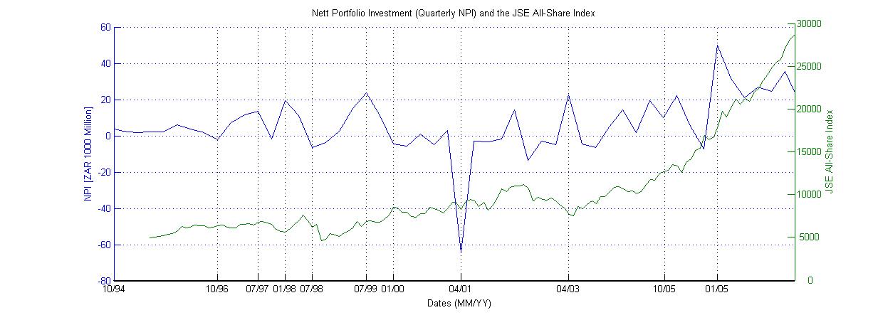
Figure 2: Net portfolio investment (NPI) flows to South Africa, 1994-2007 [Source: South African Reserve Bank] and JSE All-share Index

1. 1994: The start of the period coincided with a huge increase in NPI. The Small portfolio was most dramatically affected, followed by the Value portfolio. Here we see a dramatic increase in investment in these parts of the market, followed by equally dramatic declines in returns by 1996, correlated to the ZAR currency crisis of that period and highlighting the fragility of small caps under volatile NPI. The rank component of the Small portfolio dominates returns initially and then collapses. A large rank component indicates that as stocks move up in rank there is a large difference between their new market weights and the weights of stocks occupying their former ranks.

2. Negative NPI in 4th quarter of 1996: This was the first NPI outflow after 1994. Here negative NPI lags the dramatic 1996 ZAR currency depreciation. The latter cannot be attributed to any obvious macroeconomic signals such as increase in inflation (which was in fact decreasing at that time) or increase in unemployment, but instead seems to have been triggered by negative sentiment on the new governments performance [6]. The ZAR crisis can therefore explain both the reduction in NPI and the dramatic fall-off in the Small and Value portfolios. This period is also the beginning of a steady improvement in Mid cap stocks, some of which were Small caps in the preceding period.

3. Peak in NPI by 3rd quarter of 1997: This lags a peak in the Value portfolio that year but leads peaks in the performance of Small and Mid portfolios and leads peaks in the distributional and rank components of Small, Mid and Value portfolios.

4. Peak in NPI in 1st quarter of 1998: This leads an increase in the performance of the Mid portfolio.

5. Negative NPI in 3rd quarter of 1998: This leads a fall in the Small portfolio

6. Peak in NPI in 3rd quarter of 1999: This lags a peak in Value and all its components, but leads an improvement in the Small portfolio.

7. Negative NPI in 1st quarter of 2000: This leads a fall in the Value portfolio.

8. Plummet in NPI in 2nd quarter of 2001: This can be attributed to the collapse of the Dot-com bubble. It lagged negative trends in Small and Mid portfolios and components thereof, but preceded negative performance of the Value portfolio.

9. Significant peak by end of 1st quarter of 2003: This coincided with peaks in all portfolios and their distributional components.

10. Significant NPI drop by 4th quarter of 2005: This can be attributed to a big drop in US equity values at that time.

11. Dramatic increase in NPI at the start of 2006: This has limited discernable impact as investment in the JSE from with in SA increased dramatically. The increase in NPI and overall market value led to an improved performance of the Small portfolio.

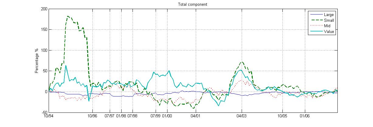
Figure 3: Total component

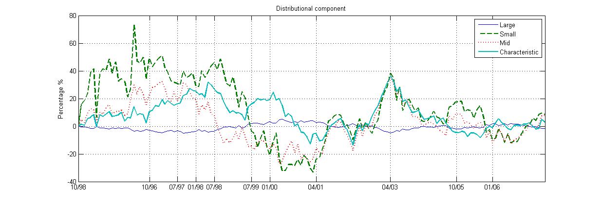
Figure 4: Rank component

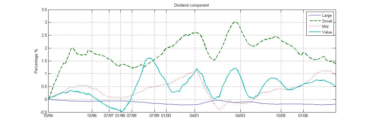
Figure 5: Distribution component as rolling annual returns.

Figure 6: Dividend component

6.1 Relative performances of rank-based portfolios and components

The next sequence of figures illustrate the relative portfolio performances, namely Small to Large, Mid to Large, Small to Mid and Small to Value. As before there are no immediately obvious trends. Instead notable regime changes can be understood in the context of exogenous impacts, including significant changes in NPI flows. As before, the beginning of the date range sees the Small cap portfolio and its components dominating the market. Next, Figure  10 corroborates that Mid cap stocks start to outperform other parts of the market after the 1996 currency crisis and brief NPI reversall. Large porfolios begin to fare better relative to Small and Mid after the Asian crisis and up to the Dotcom bubble. After the market resumes aggregate growth in 2003, triggered by an initial jump in NPI in the second quarter of that year, growth takes place in all parts of the market. The small contributions of the SPT components in that time suggests parallel growth across the market, as opposed to investors changing preference from one section of the market to another.

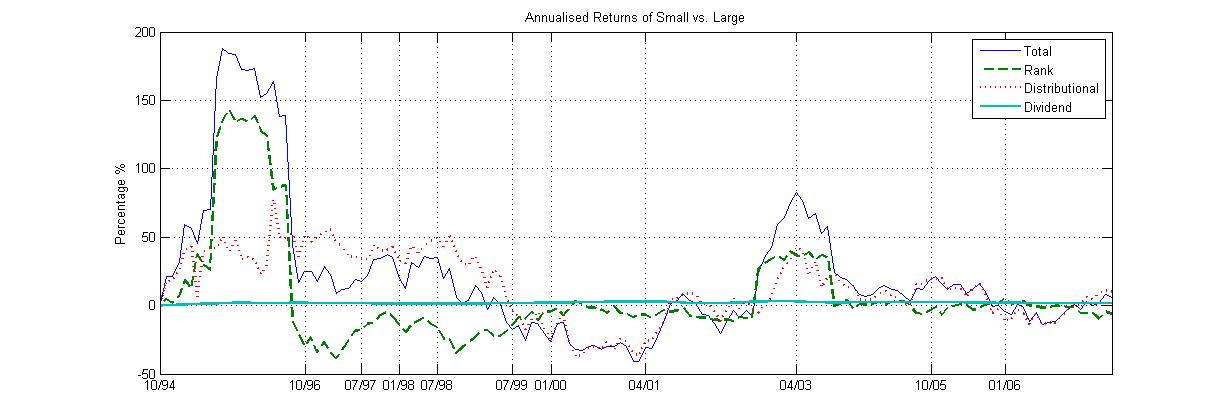
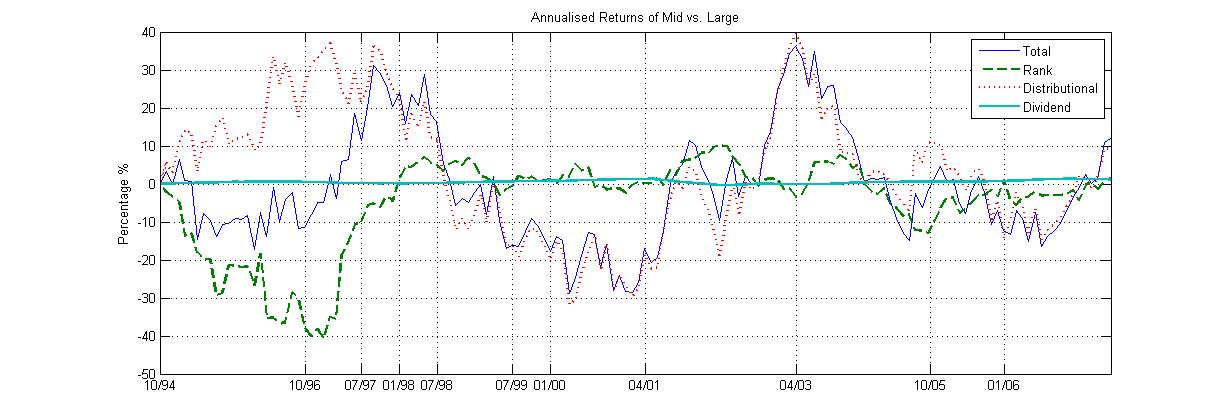
Figure 7: Components of Small relative to Large return ratios

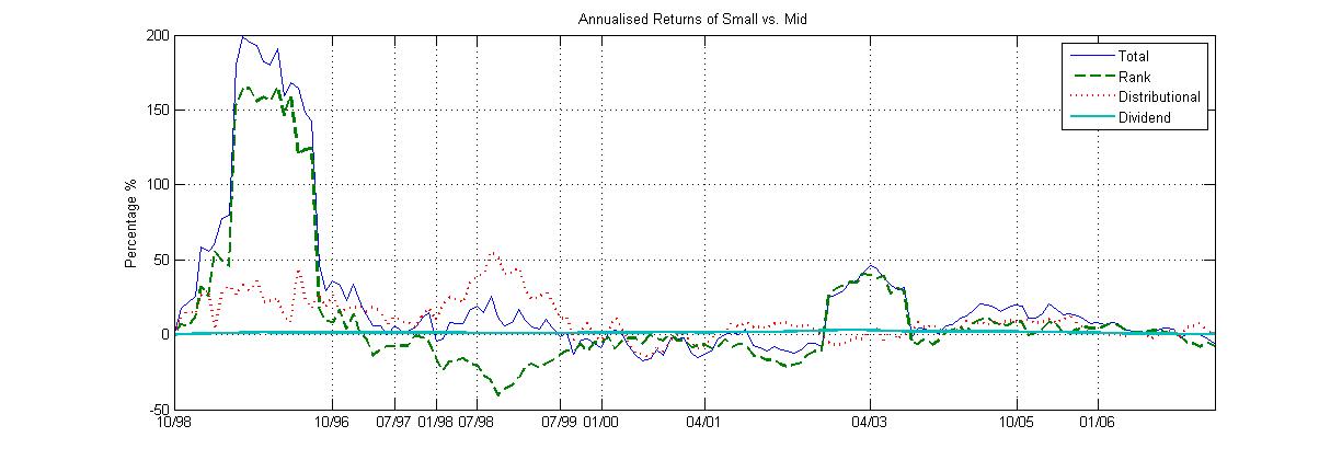
Figure 8: Components of Mid relative to Large return ratios

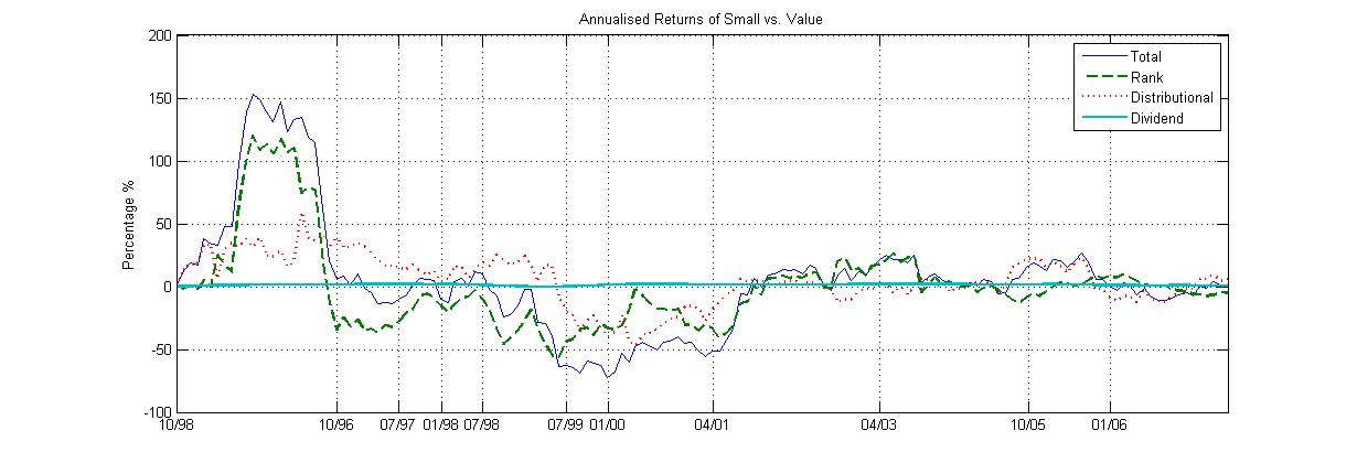
Figure 9: Components of Small relative to Mid return ratios

Figure 10: Components of Small relative to Value return ratios

6.2 Approximating the Local times

Local time components in the continuous time model are similar to rank components under the discrete equity return factorisation. However local times are strictly positive and large local times in a section of the market imply that stocks are changing rank rapidly, moving either up or down. From Equations (30) and (31) we have:

$$d\log\left({Z_{\xi}(t)\over Z_{\mu}(t)}\right) = d\log(\mu_{p_{t}(1)}(t)+\ldots+\mu_{p_{t}(k)}(t))$$ (52)

$$-\frac{1}{2}{\mu_{p_{t}(k)}(t)\over(\mu_{p_{t}(1)}(t)+\ldots+\mu_{p_{t}(k)}(t))}d\Lambda_{\log\mu_{p_{t}(k)}-\log\mu_{p_{t}(k+1)}}(t)$$

One can compute the local times for different values of $k$ from the evolution of the portfolio, $Z(t)$, and the reconstituted portfolio using the generating function $S$, by integrating the differential:

$$d\Lambda_{\log\mu_{p_{t_{0}}(k)}-\log\mu_{p_{t_{0}}(k+1)}}(t)\approx 2\left({\mu^{t_{0}}_{p_{t_{0}}(1)}+\ldots+\mu^{t_{0}}_{p_{t_{0}}(k)}\over\mu_{p_{t_{0}}(k)}^{t_{0}}}\right)$$ (53)

$$\times\left[{\log\left({{\mu_{p_{t_{1}}(1)}^{t_{1}}+\ldots+\mu_{p_{t_{1}}(k)}^{t_{1}}}\over\mu_{p_{t_{0}}(1)}^{t_{0}}+\ldots+\mu_{p_{t_{0}}(k)}^{t_{0}}}\right)}-\log\left({X_{p_{t_{0}}(1)}^{t_{1}}+\ldots+X_{p_{t_{0}}(k)}^{t_{1}}\over X_{p_{t_{0}}(1)}^{t_{0}}+\ldots+X_{p_{t_{0}}(k)}^{t_{0}}}\right)-\log\left({M^{t_{1}}\over M^{t_{0}}}\right)\right].$$ (54)

Here $\mu_{i}$ are the weights in the full market portfolio $\mu$ with value $Z_{\mu}$ and $\xi_{i}$ are the weights in the large portfolio $\xi$ for the first $k$ ranked weights and with value $Z_{\xi}$.

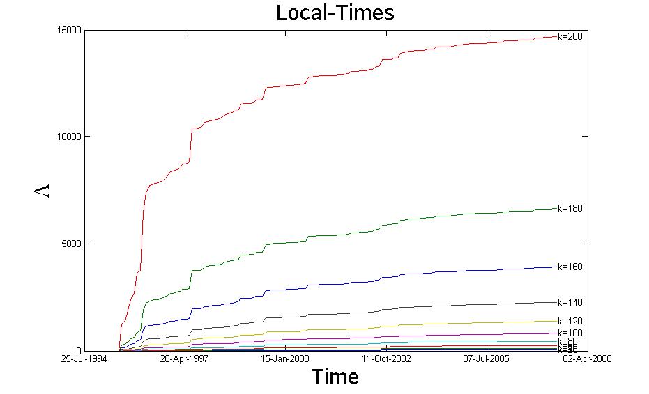
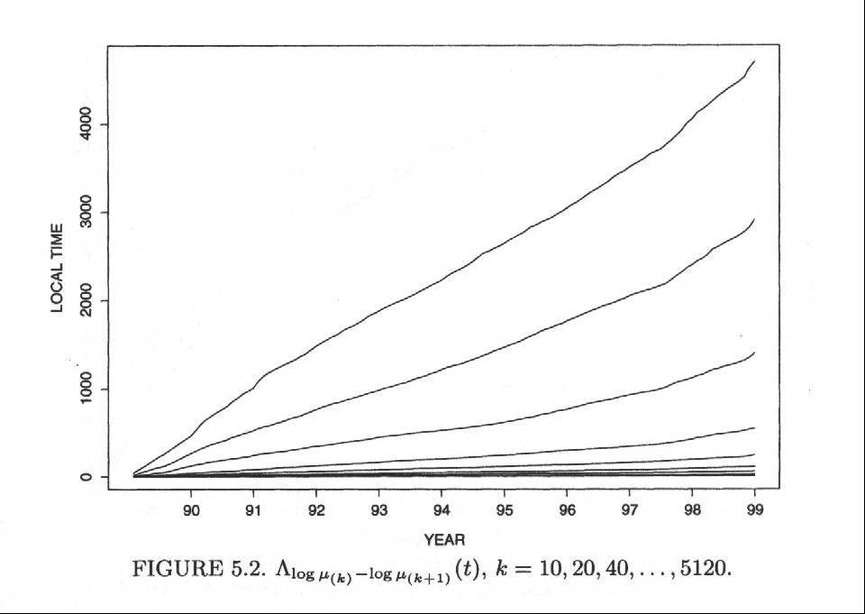
Figure 11: Local times for the largest 200 stocks on the JSE (1994-2007)

Figure 12: Local times for monthly data for the largest 5120 stocks listed in the CRSP database of US equities, 1 Jan 1990 - 31 Dec 1999[13].

In Figure  12 it is clear that the local times of small cap stocks see dramatic increments at the start of the period under investigation. This is consistent with the dramatic increase in the rank component of Small cap portfolios at that time. It suggests that relatively high NPI inflows (for that time) contributed to lots of volatility in market ranks at the Small cap end of the market. By the end of the period increments in local times flatten off throughout the market, signalling more stable market ranks. A very different situation is described in Figure  12 for the local times for US equities between 1990 and 1999 [13], where local times increase (almost) linearly. The latter implies fairly constant rates in the change of stock ranks through time.

6.3 Aggregate comparisons

Tables 1-3 document overall relative performances and contributions of components. The monthly data is decimated to consider quarterly, semi-annual and annual performances as well. We report findings for two distinct partitions of the overall stock universe, namely the case when the Large portfolio consists of the Top 10 stocks and the Small portfolio is comprised of the remaining shares in the Top 250 and the case when Large consists of the Top 40 and Small is made up of the complement of stocks in the Top 165.

Portfolio	Total	Rank	Distributional	Dividend
m=40,n=165
Small/Large	2.1 (15.8)	-2.3 (8.3)	3.7 (15.6)	0.7 (0.1)
Small/Value	-12.4 (21.1)	-9.0 (20.5)	-3.4 (10.6)	0.0 (0.2)
m=10,n=250
Small/Large	3.6 (16.7)	3.3 (7.0)	0.1 (14.9)	0.2 (0.2)
Small/Value	-1.2 (86.1)	21.1 (94.0)	-22.9 (38.5)	0.6 (0.6)

Table 1: We tabulate the components of Small and Large portfolios for 2 different partitions of the stock universe. We observe that the distributional component is dominant when the Large portfolio is comprised of the top 40 stocks and the Small portfolio is made up of the remaining stocks in the the top 165 by market capitalisation. This is a counter example to the argument that the rank contribution can be used to explain the difference of performance between Large and Small cap portfolios (which can be proved for the special case when ratios of capitalisations of Large to Small are unchanged through time). We find that if the Large portfolio is comprised of the top 10 stocks, with the remaining stocks in the top 250 making up the Small portfolio, then the rank contribution is dominant and the distributional component is much less significant.

Component	Portfolio	Monthly	Quarterly	Semi-annual	Annual
Total	Large	-0.328 (0.9)	-0.890 (1.6)	-1.759 (2.1)	-3.311 (3.1)
Total	Small	1.546 (9.9)	2.570 (9.3)	5.480 (13.7)	14.073 (23.6)
Total	Mid	-0.349 (3.9)	0.339 (6.5)	1.160 (8.5)	2.349 (11.7)
Total	Value	1.060 (5.9)	3.805 (6.8)	6.688 (13.1)	14.550 (14.6)
Distributional	Large	-0.011 (0.0)	-0.031 (0.0)	-0.060 (0.0)	-0.118 (0.1)
Distributional	Small	0.157 (0.1)	0.475 (0.2)	0.969 (0.5)	2.137 (2.4)
Distributional	Mid	0.035 (0.0)	0.098 (0.1)	0.184 (0.3)	0.263 (0.5)
Distributional	Value	0.041 (0.1)	0.123 (0.2)	0.232 (0.4)	0.386 (0.8)
Rank	Large	-0.060 (0.6)	-0.167 (1.1)	-0.345 (1.4)	-0.641 (2.2)
Rank	Small	1.104 (6.3)	2.786 (8.5)	5.652 (12.4)	10.497 (20.0)
Rank	Mid	0.271 (4.0)	0.706 (7.2)	1.379 (9.2)	2.560 (14.7)
Rank	Value	0.670 (2.8)	1.485 (4.5)	2.014 (5.3)	3.917 (8.8)
Dividend	Large	-0.258 (0.7)	-0.692 (1.2)	-1.354 (1.6)	-2.551 (2.2)
Dividend	Small	0.285 (9.1)	-0.691 (6.5)	-1.142 (7.8)	1.439 (10.8)
Dividend	Mid	-0.655 (2.4)	-0.465 (3.9)	-0.402 (5.3)	-0.475 (6.5)
Dividend	Value	0.349 (5.1)	2.197 (5.9)	4.442 (9.7)	10.248 (10.4)

Table 2: The total, distributional, rank and dividend components of the return factorisation relative to the market portfolio are tabulated. Figures are reported for the case when the Large portfolio consists of the Top 10 stocks (Top 40 in brackets) and the Small portfolio is comprised of the remaining shares in the Top 250 (Top 165). All returns are average annualised returns at the different sampling frequencies. The sampling frequencies where constructed from the original data by decimating to the required sampling rate.

Portfolio	Component	Monthly	Quarterly	Semi-annual	Annual
Small/Large	Total	22.5 (124.316843)	13.8 (40.781762)	14.5 (29.780399)	17.4 (25.820635)
Small/Large	Rank	6.5 (111.779406)	0.0 (26.856601)	0.4 (15.868101)	4.0 (10.856648)
Small/Large	Distributional	14.0 (81.085951)	11.8 (37.948269)	12.0 (27.340062)	11.1 (22.079728)
Small/Large	Dividend	2.0 (0.738672)	2.0 (0.760598)	2.1 (1.007544)	2.3 (2.469674)
Small/Value	Total	5.8 (96.082530)	-4.9 (38.792192)	-2.4 (23.799369)	-0.5 (17.555168)
Small/Value	Rank	-0.8 (91.543140)	-11.6 (30.244967)	-11.2 (22.664692)	-8.8 (13.881393)
Small/Value	Distributional	5.2 (65.417202)	5.2 (32.408844)	7.3 (18.375326)	6.6 (13.060872)
Small/Value	Dividend	1.4 (0.764702)	1.4 (0.751146)	1.5 (0.843939)	1.8 (2.083789)

Table 3: Relative portfolio performances are considered for Small vs. Large and Small vs. Value. Figures are reported for the case when the Large portfolio consists of the Top 10 stocks (Top 40 in brackets) and the Small portfolio is comprised of the remaining shares in the Top 250 (Top 165). Returns computed based on annualised values for each sampling frequency. Data at lower sampling frequencies was obtained by decimation of the original monthly data. The distributional component is more stable for Small vs. Large. The rank component is significant for Small vs. Large on shorter time-scales while for longer periods this holds for Small vs.Value portfolios (with a sign change). Small outperforms Large on all sampling rates, but only outperforms Value on the monthly time-scales. The rank contribution for Small portfolio contributes less on aggregate to total returns than for the Value portfolio.

7 Conclusion

We applied Fernholz’s stochastic portfolio factorisation to size-ranked portfolios of stocks listed on the JSE between 1994 and 2007 to tease apart rank, distributional and dividend components of total returns. We identify notable regime changes in the sentiment of investors through changes in dominating portfolios and portfolio components which correspond to changes in NPI levels rather than overall market performance.

The period under investigation coincided with several exogenous market shocks, including currency crises, which had varying impacts on different parts of the market. We highlight that outperformance of size-based portfolios can be attributed to capital allocations under significant NPI inflows. This is consistent with the perspective that, in the absence of any other information, investors pick Small cap or Mid cap portfolios in anticipation of capacity for growth. Figures  6 and  6 highlight that Small caps are also particularly vulnerable to NPI flow reversals. Our investigation confirms that NPI in a given market is often exogenously determined, with corresponding (lead) impacts on the market considered as opposed to being driven by market performance as a lagging factor.

References

- [1] Ashman, S., Fine, B., Newman, S., (2011) Amnesty International? The Nature, Scale and Impact of Capital Flight from South Africa, Journal of Southern African Studies, 37:01, 7-25
- [2] Ball, R., (1978), Anomalies in Relationships Between Securities’ Yields and Yield-Surrogates, Journal of Financial Economics 6, 103-26.
- [3] Banz, R., (1981) The Relationship Between Return and Market Value of Common Stock, Journal of Financial Economics, 9, 3-18.
- [4] Basu, S., (1977), Investment Performance of Common Stocks in Relation to their Price-Earnings Ratio: A Test of the Efficient Market Hypothesis, Journal of Finance, 32, June, 663-682.
- [5] Colander, D., Föllmer, H., Haas, A., Goldberg, M., Juselius, K., Kirman, A., Lux, T., Sloth, B., (2009) The Financial Crisis and the Systemic Failure of Academic Economics, Kiel Working Paper 1489
- [6] Diamond, A., Manning, S., Vasquez, J., Whitaker, E., (2003) South African Trade-Offs among Depreciation, Inflation, and Unemployment, Working paper
- [7] Eichgreen, B., (2013) Currency War on International Policy Coordination? Working paper
- [8] Fama, E., French, K., (1992) The cross-section of expected returns, Journal of Finance, 47, 427-465
- [9] Fama, E., French, K., (1996) Multifactor explanations of asset pricing anomalies, Journal of Finance, 51, 55-87
- [10] Fernholz, R., Shay, B., (1982) Stochastic Portfolio Theory and Stock Market Equilibrium Journal of Finance, 37, 2, 615-624
- [11] Fernholz, R., (1998) Cross-overs, dividends, and the size effect, Financial Analyst Journal 54(3) 73-78
- [12] Fernholz, R., (2001) Equity portfolios generated by functions of ranked market weights, Finance and Stochastics 5, 469-486
- [13] Fernholz, R., Stochastic Portfolio Theory, Springer - Applications of Mathematics, 2002
- [14] French, J.J., (2011) The dynamic interaction between foreign equity flows and returns: Evidence from the Johannesburg Stock Exchange, International Journal of Business and Finance Research, Vol. 5, No. 4, 45-56
- [15] Gebbie, T., Wilcox, D., (2008) Faking value and Size, Collective Insights, Special Issue (Myth-busters) of Financial Mail, Nov 2009.
- [16] Lintner, J. (1965), The valuation of risk assets and the selection of risky investments in stock portfolios and capital budgets, Review of Economics and Statistics, 47 (1), 13-37.
- [17] McCauley, R., (2012) Risk-on/Risk-off, capital flows, leverage and safe assets, BIS Working Papers, N0. 382
- [18] Mohamed, S., The impact of international capital flows on the South Africa economy since the end of Apartheid, http://www.policyinnovations.org/ideas/policy_library/data/01386/
- [19] Mossin, J. (1966), Equilibrium in a Capital Asset Market, Econometrica, Vol. 34, No. 4, pp. 768-783.
- [20] Rogoff, K., Reinhart, C., (2003) FDI to Africa: The Role of Price Stability and Currency Instability, IMF Working Paper, WP/03/10
- [21] Ross, S., (1976) The arbitrage theory of capital asset pricing, Journal of Economic Theory 13, 341-60.
- [22] Sharpe, W. F., (1964) Capital asset prices: A theory of market equilibrium under conditions of risk, Journal of Finance, 19 (3), 425-442
- [23] Svetlova, E., van Elst, H., (2012) How is non-knowledge represented in economic theory, arXiv:1209.2204v1 [q-fin.GN]
- [24] Treynor, J.L. (1962), Toward a Theory of Market Value of Risky Assets, Unpublished manuscript, final version published in 1999, in Asset Pricing and Portfolio Performance: Models, Strategy and Performance Metrics, Korajczyk, R.A. (editor), London: Risk Books, pp. 15-22.