Radiation Transport for Explosive Outflows: A Multigroup Hybrid Monte Carlo Method

Abstract

We explore Implicit Monte Carlo (IMC) and Discrete Diffusion Monte Carlo (DDMC) for radiation transport in high-velocity outflows with structured opacity. The IMC method is a stochastic computational technique for nonlinear radiation transport. IMC is partially implicit in time and may suffer in efficiency when tracking Monte Carlo particles through optically thick materials. DDMC accelerates IMC in diffusive domains. Abdikamalov extended IMC and DDMC to multigroup, velocity-dependent transport with the intent of modeling neutrino dynamics in core-collapse supernovae. Densmore has also formulated a multifrequency extension to the originally grey DDMC method. We rigorously formulate IMC and DDMC over a high-velocity Lagrangian grid for possible application to photon transport in the post-explosion phase of Type Ia supernovae. This formulation includes an analysis that yields an additional factor in the standard IMC-to-DDMC spatial interface condition. To our knowledge the new boundary condition is distinct from others presented in prior DDMC literature. The method is suitable for a variety of opacity distributions and may be applied to semi-relativistic radiation transport in simple fluids and geometries. Additionally, we test the code, called SuperNu, using an analytic solution having static material, as well as with a manufactured solution for moving material with structured opacities. Finally, we demonstrate with a simple source and 10 group logarithmic wavelength grid that IMC-DDMC performs better than pure IMC in terms of accuracy and speed when there are large disparities between the magnitudes of opacities in adjacent groups. We also present and test our implementation of the new boundary condition.

1. Introduction

Type Ia supernovae (SNe Ia) are thermonuclear explosions of carbon-oxygen white dwarf stars. A variety of models have been proposed for SNe Ia. In all of these models, the expansion becomes ballistic and homologous within $\sim$100 seconds. Gamma rays from the radioactive decay of ⁵⁶Ni formed in the explosion heat the expanding ejecta, making it glow for weeks. Two remarkable features of Type Ia supernova (SN Ia) light curves are that their peak luminosities span a modest range and that they can be calibrated to be standard candles, making them useful for measuring distances in the universe [see, e.g., Riess et al. (1998); Perlmutter et al. (1999)].

SN Ia light curves and spectra are the result of complex radiative processes involving the interaction of photons with millions of spectral lines in various stages of ionization, including strong scattering effects, in the asymmetric, chemically inhomogeneous, quasi-relativistically expanding ejecta [see, e.g., Kasen et al. (2006); Baron & Hauschildt (2007); van Rossum (2012)].

Nevertheless, if provided with quality material data, a robust numerical radiation transport method that is amenable to parallelization and is efficient in optically thick regions of phase space should be able to reproduce SN Ia spectra and light curves. Monte Carlo (MC) is a simple approach to transport computation that allows one to model “bundles” of photons directly as particle histories. Particle processes are carried out stochastically with random number sampling (Lewis & Miller, 1993, p. 296). Each of these histories is independent from the others; hence Monte Carlo can be performed in parallel and in domain decomposed settings.

Implicit Monte Carlo (IMC) is an MC technique for solving the time dependent radiation transport equation coupled nonlinearly with material (Fleck & Cummings, 1971). In implementation, a non-dimensional quantity resulting from temporal discretization of the material equation dictates how likely a Monte Carlo particle can be absorbed or re-emitted instantaneously. The non-dimensional quantity is referred to as the Fleck factor. The instantaneous absorption-reemission event in an IMC time step can be modeled as an effective inelastic scattering event for each particle history.

The semi-implicitness of IMC provides an advantage over explicit radiation transport methods by mitigating Courant-type instabilities due to large time steps and optically thick domains (Fleck & Cummings, 1971). This advantage is obtained through the isotropic effective scattering events mentioned above. Explicit transport methods incur these errors from having to instantiate the entire emission energy as particles at the beginning of the time step. With IMC, a large time step and a strong absorption opacity allow effective scattering to dominate MC particle-material grid interactions.

A significant drawback of IMC is the computational inefficiency of having to model instantaneous remission through effective scattering in optically thick regimes. Both effective and physical scattering can be partly avoided by hybridizing IMC with a diffusion method. This diffusion routine can either be deterministic or stochastic. Fleck & Canfield (1984) incorporate Random Walk (RW) to replace small scattering steps with large diffusion steps. These large diffusion steps assume a particle has undergone several collisions and may be isotropically placed on a sphere centered at the particle’s initial position. The diffusion sphere radius is bounded by the cell in which the particle resides. As Densmore and others note (Densmore et al., 2007, 2012), the RW method must use transport for particles near spatial cell boundaries even in optically thick domains; so its ability to increase IMC efficiency is limited.

Discrete Diffusion Monte Carlo (DDMC) (Densmore et al., 2007, 2008, 2012) and Implicit Monte Carlo Diffusion (IMD) (Gentile, 2001; Cleveland et al., 2010) are recent alternatives to Random Walk that lend a stochastic interpretation to the discretized diffusion equation. Consequently in either method, a diffusion Monte Carlo particle’s position is fundamentally ambiguous within the spatial cell where it resides. The core difference between IMD and DDMC is the treatment of particle histories. In IMD, the diffusion equation is discrete in time and there is a probability to determine completion of each time step (Cleveland et al., 2010). DDMC treats particle times continuously, removing causal ambiguity when interfaced or hybridized with IMC (Densmore et al., 2007).

Multifrequency Implicit Monte Carlo-Discrete Diffusion Monte Carlo (IMC-DDMC) methods have very recently been formulated by Densmore et al. (2012) and Abdikamalov et al. (2012). Densmore’s formulation is for local thermodynamic equilibrium (LTE) photon transport with an opacity dependence on frequency that is roughly monotonic. Specifically, it is assumed that the opacity is optically thick at low photon frequency and can be modeled with grey DDMC while multifrequency IMC is applied above a user-defined frequency threshold. This frequency threshold depends heuristically on the cell-local material properties. In practice, this cutoff can be achieved approximately on a group structure by lumping adjacent groups that are sufficiently diffuse into one large DDMC group.

The formulation of Abdikamalov et al. (2012) is for neutrino transport in either static or velocity-dependent material. The frequency effects are treated with a multigroup approach and, similarly to the approach of Densmore et al. (2012), a heuristic determines whether IMC or DDMC is applied at a specific spatial cell and frequency group.

Here, we present an extension of IMC-DDMC to photon transport in SNe Ia that is similar to that of Abdikamalov et al. (2012) for neutrino transport in core collapse supernovae. In contrast to the work of Abdikamalov et al. (2012), we treat velocity as linearly continuous at the sub-cell level; we test an IMC-DDMC-specific algorithm to account for spatial grid motion; we only apply first-order relativity to both IMC and DDMC; we derive a new IMC-DDMC boundary condition for semi-relativistic outflow; and we describe methods for non-uniform group structuring that extend formulae presented by Densmore et al. (2012). We also make note of the consequence of DDMC particle frequency ambiguity in Doppler shifting over multigroup structures. As done by Kasen et al. (2006), we exploit the homologous relation between space and fluid expansion time and formulate the method over a velocity grid. Additionally, we use the Method of Manufactured Solutions (Oberkampf & Roy, 2010, p. 219) to verify SuperNu’s ability to reproduce radiation energy density profiles with appropriate sources and initial conditions.

To our knowledge, the modification to the standard IMC-DDMC boundary condition described in Section 2.3 is a novel theoretical finding. Specifically, we obtain an additional term that multiplies the probability an IMC particle incident on a DDMC region will convert to DDMC. This factor is singular for incident particles that have comoving directions lying in the tangent plane of the IMC-DDMC boundary at the particle’s point of contact. However, we show the expected IMC energy current reflected and transmitted from and into the DDMC region is finite. Since the singularity does not introduce infinities in energy balance, we suppose that the new quantity may be interpreted as an IMC particle weight modification.

This paper is organized as follows. In Section 2, we discuss the IMC-DDMC theory and implementation. We first discuss the treatment of fluid coupling and relativistic effects; in Section 2.1, we review and formulate IMC for lab frame transport on a velocity grid; in Section 2.2, we review and discuss DDMC; in Section 2.3, we then perform an asymptotic analysis on a moving surface to obtain the new boundary condition; in Section 2.4, we move the discussion to coupling IMC and DDMC over a high-velocity Lagrangian grid. In Section 3.1, we exhibit a closed form verification test for static material radiation transport. This test is an extension of the thermally coupled P₁ solutions provided by McClarren et al. (2008a) to account for rudimentary multifrequency. In Section 3.2, we test our implementation of IMC-DDMC against a manufactured solution that includes outflow and a multigroup structure. The manufactured solution is constructed to counteract some recognized properties of radiation trapped in high velocity, spherical flow such as inverse quartic dependence of energy density on the Eulerian radius (Mihalas & Mihalas, 1984, p. 474). In Section 3.3, we test the efficiency of IMC-DDMC relative to pure IMC for group structures of varying contrast ratios between alternating thick-thin grouped opacity values. Also in Section 3.3, we demonstrate a discrepancy between IMC-DDMC and pure IMC may form at IMC-DDMC interfaces for high velocity outflows. We find this error to be large for IMC-DDMC thresholds on the order of 10 mean free paths per cell per group in the set of Heaviside source problems discussed (in other words, when IMC is applied in a cell and group with fewer than 10 mean free paths across some cell length measure and DDMC is applied otherwise). We implement the new boundary condition in IMC-DDMC and test its ability to counteract the redshift-induced error for coupling thresholds equal to 3 mean free paths and to 10 mean free paths per cell per group. Finally in Section 4, we summarize our findings, discuss possible future work, and discuss the feasibility of the general multifrequency treatment of IMC-DDMC.

2. Homologous Velocity Space IMC-DDMC

The derivation of IMC-DDMC and IMC-IMD in a multigroup setting has been discussed extensively in prior publications (Cleveland et al., 2010; Densmore et al., 2012; Abdikamalov et al., 2012). We briefly review the relevant method derivations and discuss the distinctive algorithmic features we have implemented to reconcile IMC-DDMC with a ballistic fluid on a Lagrangian grid. Subsequently, we describe an optimization method we will refer as “group lumping”, Eqs. (72)-(74). Group lumping combines adjacent groups that are heuristically deemed DDMC-appropriate into larger groups. Hence the method is a natural extension to methods that model all radiation below a frequency threshold with grey DDMC (Densmore et al., 2012). It is evident from theory that group lumping over optically-thick regions in phase space will increase the overall code efficiency.

As Pomraning and Castor have done, we denote comoving quantities with a subscript 0 and leave the corresponding lab (or outflow center) frame quantities unsubscripted. The thermal radiative transport equation without external sources in the lab frame is (Pomraning, 1973; Castor, 2004)

$$\frac{1}{c}\frac{\partial I_{\nu}}{\partial t}+\hat{\Omega}\cdot\nabla I_{\nu}+\sigma_{\nu,a}I_{\nu}=\sigma_{\nu,a}B_{\nu}-\sigma_{\nu,s}I_{\nu}+\\ \int_{4\pi}\int_{0}^{\infty}\frac{\nu}{\nu^{\prime}}\sigma_{s}(\vec{r},\nu^{\prime}\rightarrow\nu,\hat{\Omega}^{\prime}\rightarrow\hat{\Omega})I_{\nu^{\prime}}(\vec{r},\hat{\Omega}^{\prime},t)d\nu^{\prime}d\Omega^{\prime}$$ (1)

where $\vec{r}$ is the spatial coordinate, $\hat{\Omega}$ is a unit direction, $t$ is time, $\nu$ is frequency, $c$ is the speed of light, $I_{\nu}$ is the radiation intensity, and $B_{\nu}$ is the lab frame thermal emission. If the fluid is static, $B_{\nu}(\hat{\Omega})=B_{0,\nu_{0}}$ is the Planck function (Pomraning, 1973, p. 156). Anisotropies in the radiation field due to fluid motion are represented in the opacities and intensities in Eq. (1).

For a radiative hydrodynamic system, the Euler equations that couple with Eq. (1) are (Castor, 2004, p. 85)

$$\frac{\partial\rho}{\partial t}+\nabla\cdot(\rho\vec{U})=0\;\;,$$ (2)

$$\frac{\partial(\rho\vec{U})}{\partial t}+\nabla\cdot(\rho\vec{U}\vec{U})+\nabla P=-\vec{g}\;\;,$$ (3)

and

$$\frac{\partial}{\partial t}\left(\rho e+\frac{1}{2}\rho U^{2}\right)+\nabla\cdot\left(\rho\vec{U}(e+P/\rho)+\frac{1}{2}\rho\vec{U}U^{2}\right)=-g^{(0)}$$ (4)

where $e$, $\rho$, $\vec{U}$, and $P$ are the internal energy, density, velocity, and pressure of the fluid in the lab frame (an inertial frame not following any particular fluid parcel). The 4-vector $(g^{(0)},\vec{g})$ is the radiation energy-momentum coupling (Castor, 2004, p. 109). The superscript, (0), denotes the time component of the 4-vector. We are interested in tracking changes to the material in the comoving or Lagrangian coordinate of velocity cells. The Lagrangian equation corresponding to Eq. (4) is (Castor, 2004, pp. 5-10)

$$\rho\frac{De}{Dt}+P\nabla\cdot\vec{U}=-g^{(0)}$$ (5)

where the operator $D/Dt$ is the Lagrangian derivative. The second term on the left-hand-side of equation (5) is usually negligible relative to $g^{(0)}$ in the physical regimes of interest. In a homologous outflow, $\nabla\cdot\vec{U}=3/t_{\text{exp}}$ where $t_{\text{exp}}$ is the fluid expansion time. The ratio of the rate of adiabatic, ideal gas cooling to the thermal radiation deposition rate is approximately $\Lambda=\displaystyle\frac{3N_{A}k}{M_{A}aT^{3}}\frac{\rho/c\sigma_{P}}{t_{\text{exp}}}$ where $N_{A}$, $k$, $M_{A}$, $T$, and $\sigma_{P}$ are Avogadro’s number, Boltzmann’s constant, molar mass, temperature, and Planck opacity, respectively (Kasen et al., 2006). For an outflow of Nickel with $T=12,000$ K, $\sigma_{P}=0.1\rho$ cm^-1, and $t_{\text{exp}}=10$ days, the ratio is approximately $\Lambda\approx 1.3\times 10^{-7}$. As Kasen et al. (2006) argue, $\Lambda$ remains small over the times of interest in light curve and spectra observation for Type Ia SNe. Our outflow simulations employ numbers that generate small $\Lambda$. So we neglect the adiabatic cooling rate of the gas, $P\nabla\cdot\vec{U}$, in our subsequent analysis. We do not extend this approximation to photons; the adiabatic cooling in the radiation field is a large factor in our velocity-dependent simulations. The analysis provided agrees with arguments by Pinto & Eastman (2000) as well.

The Lagrangian momentum equation is (Castor, 2004, p. 9)

$$\rho\frac{D\vec{U}}{Dt}+\nabla P=-\vec{g}\;\;.$$ (6)

The velocity across a cell (or discrete fluid parcel) will not change in the Lagrangian frame; hence the first term of Eq. (6) on the left-hand-side will be zero in the homologous outflow. Additionally, we assume the pressure gradient across the fluid parcel will be small. Consequently $\vec{g}=0$. So $g_{0}^{(0)}=g^{(0)}-\vec{U}\cdot\vec{g}/c^{2}\approx g^{(0)}$. With the above simplifications, Eq. (5) becomes (Szőke & Brooks, 2005)

$$C_{v}\frac{DT}{Dt}=-g_{0}^{(0)}=-g_{0,a}^{(0)}-g_{0,s}^{(0)}=\\ \int_{4\pi}\int_{0}^{\infty}\sigma_{0,\nu_{0},a}(I_{0,\nu_{0}}-B_{0,\nu_{0}})d\nu_{0}d\Omega_{0}\\ +\int_{4\pi}\int_{0}^{\infty}\sigma_{0,\nu_{0},s}I_{0,\nu_{0}}d\nu_{0}d\Omega_{0}-\int_{4\pi}\int_{0}^{\infty}\int_{4\pi}\int_{0}^{\infty}\ldots\\ \frac{\nu_{0}}{\nu_{0}^{\prime}}\sigma_{0,s}(\vec{r},\nu_{0}^{\prime}\rightarrow\nu_{0},\hat{\Omega}_{0}^{\prime}\cdot\hat{\Omega}_{0})I_{0,\nu_{0}^{\prime}}d\nu_{0}^{\prime}d\Omega_{0}^{\prime}d\nu_{0}d\Omega_{0}\;\;,$$ (7)

where $C_{v}$ is the heat capacity per unit volume, $g_{0,a}^{(0)}$ ($g_{0,s}^{(0)}$) includes all absorption (scattering) terms, and

$$\sigma_{0,\nu_{0},s}=\int_{4\pi}\int_{0}^{\infty}\sigma_{0,s}(\vec{r},\nu_{0}\rightarrow\nu_{0}^{\prime},\hat{\Omega}_{0}\cdot\hat{\Omega}_{0}^{\prime})d\nu_{0}^{\prime}d\Omega_{0}^{\prime}\;\;.$$ (8)

Equation (7) is amenable to the usual IMC temporal discretization (Fleck & Cummings, 1971; Abdikamalov et al., 2012). The coupling, however, is in the comoving frame and Eq. (1) is in the lab frame. If the fluid field is nowhere accelerating, the comoving transport equation to first order is (Castor, 2004, p. 110)

$$(1+\hat{\Omega}_{0}\cdot\vec{U}/c)\frac{1}{c}\frac{DI_{0,\nu_{0}}}{Dt}\\ +\hat{\Omega}_{0}\cdot\nabla I_{0,\nu_{0}}-\frac{\nu_{0}}{c}\hat{\Omega}_{0}\cdot\nabla\vec{U}\cdot\nabla_{\nu_{0}\hat{\Omega}_{0}}I_{0,\nu_{0}}\\ +\frac{3}{c}\hat{\Omega}_{0}\cdot\nabla\vec{U}\cdot\hat{\Omega}_{0}I_{0,\nu_{0}}=\sigma_{0,\nu_{0},a}(B_{0,\nu_{0}}-I_{0,\nu_{0}})-\sigma_{0,\nu_{0},s}I_{0,\nu_{0}}\\ +\int_{4\pi}\int_{0}^{\infty}\frac{\nu_{0}}{\nu_{0}^{\prime}}\sigma_{0,s}(\vec{r},\nu_{0}^{\prime}\rightarrow\nu_{0},\hat{\Omega}_{0}^{\prime}\cdot\hat{\Omega}_{0})I_{0,\nu_{0}^{\prime}}d\nu_{0}^{\prime}d\Omega_{0}^{\prime}\;\;,$$ (9)

where in Castor’s notation $\nabla_{\nu_{0}\hat{\Omega}_{0}}$ is the comoving momentum derivative for photons.

2.1. Lab Frame IMC

Applying the IMC discretization to Eqs. (7) and (9) and expressing the re-balanced equations in differential form (Densmore et al., 2012) gives

$$C_{v}\frac{DT}{Dt}=\\ f_{n}\left(\int_{4\pi}\int_{0}^{\infty}\sigma_{0,\nu_{0},a,n}I_{0,\nu_{0}}d\nu_{0}d\Omega_{0}-\sigma_{P,n}acT_{n}^{4}\right)-g_{0,s}^{(0)}$$ (10)

and

$$(1+\hat{\Omega}_{0}\cdot\vec{U}/c)\frac{1}{c}\frac{DI_{0,\nu_{0}}}{Dt}+\hat{\Omega}_{0}\cdot\nabla I_{0,\nu_{0}}\\ -\frac{\nu_{0}}{c}\hat{\Omega}_{0}\cdot\nabla\vec{U}\cdot\nabla_{\nu_{0}\hat{\Omega}_{0}}I_{0,\nu_{0}}+\frac{3}{c}\hat{\Omega}_{0}\cdot\nabla\vec{U}\cdot\hat{\Omega}_{0}I_{0,\nu_{0}}\\ +(\sigma_{0,\nu_{0},s,n}+\sigma_{0,\nu_{0},a,n})I_{0,\nu_{0}}=\frac{f_{n}}{4\pi}\sigma_{0,\nu_{0},a,n}b_{0,\nu_{0},n}acT_{n}^{4}\\ +\frac{b_{0,\nu_{0},n}\sigma_{0,\nu_{0},a,n}}{4\pi\sigma_{P,n}}(1-f_{n})\int_{4\pi}\int_{0}^{\infty}\sigma_{0,\nu_{0}^{\prime},a,n}I_{0,\nu_{0}^{\prime}}d\nu_{0}^{\prime}d\Omega_{0}^{\prime}\\ +\int_{4\pi}\int_{0}^{\infty}\frac{\nu_{0}}{\nu_{0}^{\prime}}\sigma_{0,s,n}(\vec{r},\nu_{0}^{\prime}\rightarrow\nu_{0},\hat{\Omega}_{0}^{\prime}\cdot\hat{\Omega}_{0})I_{0,\nu_{0}^{\prime}}d\nu_{0}^{\prime}d\Omega_{0}^{\prime}\;\;,$$ (11)

where the integer subscript $n$ denotes quantities evaluated at the beginning of a time step. The value $g_{0,s}^{(0)}$ has been lumped entirely into the material equation since physical scattering generally admits direct treatment in MC transport. $P$,$R$ and $g$ subscripts indicate Planck, Rosseland or grouped quantities, respectively. The opacities are evaluated in the comoving frame. The value $b_{0,\nu_{0}}$ is the frequency-normalized Planck function in the comoving frame, and the Fleck factor $f_{n}$ (Fleck & Cummings, 1971) is

$$f_{n}=\frac{1}{1+\alpha\beta_{n}\sigma_{P,n}c\Delta t_{n}}\;\;.$$ (12)

The value $\alpha\in[0,1]$ is a time centering control parameter (often set to 1), $\beta_{n}=4aT_{n}^{3}/C_{v,n}$ and $\Delta t_{n}$ is the physical time step size for time step $n$. The second term on the right-hand-side of Eq. (11) is the source due to effective scattering (Fleck & Cummings, 1971; Densmore et al., 2012). The differential effective scattering opacity, $(1-f_{n})b_{0,\nu_{0},n}\sigma_{0,\nu_{0},a,n}\sigma_{0,\nu_{0}^{\prime},a,n}\nu_{0}^{\prime}/4\pi\sigma_{P,n}\nu_{0}$, is separable in $\nu_{0}$ and $\nu_{0}^{\prime}$; so the new frequency of a photon undergoing effective scattering is probabilistically independent of the old frequency (Mihalas & Mihalas, 1984, p. 327).

Equation (11) could in principle be replaced with the fully relativistic comoving transport equation described by (Mihalas & Mihalas, 1984, p. 434). Here, we consider only first order relativistic effects but note that higher order effects could be incorporated with relative ease in MC codes (Abdikamalov et al., 2012). The typical outflow speed of Type Ia SNe is approximately $U_{\max}=30,000$ km/s, so $(U_{\max}/c)^{2}\approx 0.01$. The lab frame Eulerian coordinate is related to the velocity through

$$\vec{r}=\vec{U}(t_{n}+t_{\min})\;\;,$$ (13)

where $t_{n}=\sum_{n^{\prime}=1}^{n-1}\Delta t_{n}$ and $t_{\min}$ is the starting time of the expansion.

The right hand side of Eq. (11) implies source MC particles may be generated, scattered, or absorbed in the comoving frame in the same manner as the static material IMC method (Abdikamalov et al., 2012; Lucy, 2005). To seed interaction locations between events in a particle’s history, the particle’s properties may be mapped to the lab frame and streamed by Eq. (1). Neglecting all terms of order $U^{2}/c^{2}$ or higher, the frequency and direction transformations are (Castor, 2004, p. 103)

$$\nu=\nu_{0}\left(1+\frac{\hat{\Omega}_{0}\cdot\vec{U}}{c}\right)$$ (14)

and

$$\hat{\Omega}=\frac{\hat{\Omega}_{0}+\vec{U}/c}{1+\hat{\Omega}_{0}\cdot\vec{U}/c}$$ (15)

respectively. The cumulative effect of these transformations in each particle history accounts for Doppler shifting and aberration in the MC process (Lucy, 2005). According to (Pomraning, 1973, p. 156) and (Castor, 2004, p. 104), the opacity in the lab frame is

$$\sigma_{\text{lab}}=\frac{\nu_{0}}{\nu}\sigma_{\text{cmf}}\;\;,$$ (16)

where “cmf” stands for comoving frame. A computational convenience may be taken by virtue of Eq. (13). Following Kasen, we track both IMC and DDMC particles in velocity space. Thus, the grid itself is logically unchanging and velocity acts as a Lagrangian coordinate. IMC particles move over “velocity distances” denoted with a lower case $u$. Corresponding to physical distance in standard IMC (Fleck & Cummings, 1971), there is a velocity to a cell boundary $u_{b}$, a velocity to collision $u_{\text{col}}$, and a velocity distance to census at the end of a time step $u_{\text{cen}}$. Through Eq. (13), the velocity to a boundary can be calculated with the same formula as the physical distance and is consequently dependent on grid geometry. For the $u_{\text{col}}$ and $u_{\text{cen}}$, the formulas are

$$u_{\text{col}}=\frac{-\ln(\xi)}{(t_{n}+t_{\min})(1-\hat{\Omega}_{p}\cdot\vec{U_{p}}/c)(\sigma_{s,n}+\sigma_{a,n})}$$ (17)

and

$$u_{\text{cen}}=c\left(\frac{t_{n}+\Delta t_{n}-t_{p}}{t_{n}+t_{\min}}\right)$$ (18)

where $t_{p}$, $\vec{U}_{p}$, and $\hat{\Omega}_{p}$ are a particle’s time, “velocity position”, and direction in the lab frame, respectively. The value $\xi\in(0,1]$ is a uniformly sampled random number. The minimum $u=\min(u_{\text{col}},u_{\text{cen}},u_{b})$ indicates which event occurs at each iteration of a particle’s history.

Effective absorption can be alternatively calculated with implicit capture (Lewis & Miller, 1993, p. 332). If implicit capture is used to reduce the variance of an MC particle tally, the collision velocity only includes scattering opacities (Fleck & Cummings, 1971),

$$u_{\text{col}}=\frac{-\ln(\xi)}{(t_{n}+t_{\min})(1-\hat{\Omega}_{p}\cdot\vec{U_{p}}/c)(\sigma_{s,n}+(1-f_{n})\sigma_{a,n})}\;\;.$$ (19)

The energy of a particle in the lab frame is reduced by $E_{p}\rightarrow E_{p}e^{-f_{n}\frac{\nu_{0,p}}{\nu_{p}}\sigma_{a,n}u(t_{n}+t_{\min})}$ where $\nu_{p}$ and $\nu_{0,p}$ are the particle’s lab and comoving frame frequency, respectively.

For a one dimensional, spherically symmetric shell geometry,

$$u_{b}=\begin{cases}|(U_{j-1/2}^{2}-(1-\mu_{p}^{2})U_{p}^{2})^{1/2}+\mu_{p}U_{p}|\\ \;\;\;\;\text{if }\mu_{p}<-\sqrt{1-(U_{j-1/2}/U_{p})^{2}}\\ \\ (U_{j+1/2}^{2}-(1-\mu_{p}^{2})U_{p}^{2})^{1/2}-\mu_{p}U_{p}\\ \;\;\;\;\text{otherwise}\end{cases}$$ (20)

where $\mu_{p}$ is the projection of $\hat{\Omega}_{p}$ along the radial coordinate. The index $j\in\{1\ldots J\}$ denotes a velocity zone. For a geometry in which the inner most cell has $U_{1/2}=0$, the second case in Eq. (20) must be applied for the innermost cell, $j=1$, and $\mu_{p}\in[-1,1]$. IMC particle position in velocity space must be updated to have its physical position unchanged. The censused position is simply maintained with

$$\vec{U}_{p,\text{new cen}}(t_{n}+\Delta t_{n}+t_{\min})=\vec{U}_{p,\text{old cen}}(t_{n}+t_{\min})=\vec{r}_{p,\text{cen}}\;\;,$$ (21)

where $\vec{r}_{p}$ is the implied IMC particle position at the end of a time step. Equation (21) can either be implemented before or after the routine that advances the particle set. We find that introducing a time centering parameter, $\alpha_{2}$, to split the velocity position shift before and after transport is generally preferable. At particle advance, the algorithm is

1. $\vec{U}_{p,\text{* cen}}(t_{n}+\alpha_{2}\Delta t_{n}+t_{\min})=\vec{U}_{p,\text{old cen}}(t_{n}+t_{\min})$.

2. IMC: $\vec{U}_{p,\text{* cen}}\rightarrow\vec{U}_{p,*}$.

3. $\vec{U}_{p,\text{new cen}}(t_{n}+\Delta t_{n}+t_{\min})=\vec{U}_{p,*}(t_{n}+\alpha_{2}\Delta t_{n}+t_{\min})$.

If we were transporting massive particles, then the above steps would ensure that the particle does not move in space if it has zero velocity with respect to the lab frame.

In many transport problems, the exact dependence of opacity on frequency is not necessarily known. If the fully continuous opacities are known, they may not be practical to implement in analytic form. One might then a priori posit a group structure for the opacities that are relevant to the transport problem and formulate Eq. (11) in terms of such a group structure. We may then set the group Rosseland and Planck opacities, $\sigma_{P,g,n}=\sigma_{R,g,n}=\sigma_{a,g,n}$. But if each velocity cell has its own frequency grouping and number of groups, we must constrain the resulting equation to one particular fluid cell. For a cell $j$, group index $g$, and a total number of (transport) groups $G_{j}$,

$$(1+\hat{\Omega}_{0}\cdot\vec{U}/c)\frac{1}{c}\frac{DI_{0,g}}{Dt}+\hat{\Omega}_{0}\cdot\nabla I_{0,g}\\ +\frac{1}{c}\hat{\Omega}_{0}\cdot\nabla\vec{U}\cdot\hat{\Omega}_{0}(I_{0,g}-\nu_{g-1/2}I_{0,\nu_{g-1/2}}+\nu_{g+1/2}I_{0,\nu_{g+1/2}})\\ -\frac{1}{c}\hat{\Omega}_{0}\cdot\nabla\vec{U}\cdot(\mathbf{I}-\hat{\Omega}_{0}\hat{\Omega}_{0})\cdot\nabla_{\hat{\Omega}_{0}}I_{0,g}+\frac{3}{c}\hat{\Omega}_{0}\cdot\nabla\vec{U}\cdot\hat{\Omega}_{0}I_{0,g}\\ +(\sigma_{s,g,n}+\sigma_{a,g,n})I_{0,g}=\frac{f_{n}}{4\pi}\gamma_{g,n}\sigma_{P,n}acT_{n}^{4}\\ +\frac{1}{4\pi}\gamma_{g,n}(1-f_{n})\sum_{g^{\prime}=1}^{G_{j}}\int_{4\pi}\sigma_{a,g^{\prime},n}I_{0,g^{\prime}}d\Omega_{0}^{\prime}\\ +\sum_{g^{\prime}=1}^{G_{j}}\int_{4\pi}\sigma_{s,n}(g^{\prime}\rightarrow g,\hat{\Omega}_{0}^{\prime}\cdot\hat{\Omega}_{0})I_{0,g^{\prime}}d\Omega_{0}^{\prime}\;\;,$$ (22)

where $g\in\{1\ldots G_{j}\}$, $U\in[U_{j-1/2},U_{j+1/2}]$ and $\gamma_{g,n}=\int_{\nu_{g+1/2}}^{\nu_{g-1/2}}\sigma_{a,n}b_{0,\nu_{0},n}d\nu_{0}/\sigma_{P,n}$. Additionally, $I_{0,g}=\int_{\nu_{g+1/2}}^{\nu_{g-1/2}}I_{0,\nu_{0}}d\nu_{0}$ and a higher group index corresponds to a lower frequency or equivalently a higher wavelength. $\mathbf{I}$ is the identity matrix. We have made sure to apply the group grid in the comoving frame. Equation (22) makes use of Castor’s division of the Doppler and aberration corrections from the photon momentum gradient. The third term on the left-hand-side of Eq. (22) indicates that Doppler shifting will cause particles to leak between groups. Moreover, the leakage process will depend on the anisotropy of the radiation field as well as the velocity gradient. We track frequency or wavelength continuously. Hence when an IMC particle crosses a cell boundary, its group in the subsequent cell environment can be determined without ambiguity. If groups in adjacent cells do not align, group intersections determine transitions in phase space for IMC and DDMC particles (Densmore et al., 2012). In-cell group transitions from streaming in velocity may be modeled directly by computing a velocity distance to Doppler shift, $u_{\text{Dop}}$, and taking $u=\min(u_{\text{col}},u_{\text{cen}},u_{b},u_{\text{Dop}})$. The form of the velocity to Doppler shift in a spherically symmetric outflow is $u_{\text{Dop}}=|c(1-\nu_{g+1/2}/\nu_{p})-\vec{U}_{p}\cdot\hat{\Omega}_{p}|$ where $\nu_{p}$ is particle lab frame frequency and use has been made of Eqs. (14) and (15).

2.2. Comoving Frame DDMC

Integrating Eq. (22) over comoving solid angle, using the simplifications described in Castor (2004, pp. 102-111), and assuming comoving isotropic opacities,

$$\frac{1}{c}\frac{\partial\phi_{0,g}}{\partial t}+\frac{1}{c}\nabla\cdot(\vec{U}\phi_{0,g})+\nabla\cdot\vec{F}_{0,g}+\\ (\mathbf{P}_{0,g}-\nu_{g-1/2}\mathbf{P}_{0,\nu_{g-1/2}}+\nu_{g+1/2}\mathbf{P}_{0,\nu_{g+1/2}}):\nabla\vec{U}\\ +\left[\sigma_{s,g,n}+f_{n}\sigma_{a,g,n}+(1-\gamma_{g,n})(1-f_{n})\sigma_{a,g,n}\right]\phi_{0,g}\\ =f_{n}\gamma_{g,n}\sigma_{P,n}acT_{n}^{4}+\gamma_{g,n}(1-f_{n})\sum_{g^{\prime}\not=g}^{G_{j}}\sigma_{a,g^{\prime},n}\phi_{0,g^{\prime}}\\ +\sum_{g^{\prime}=1}^{G_{j}}\sigma_{s,n}(g^{\prime}\rightarrow g)\phi_{0,g^{\prime}}$$ (23)

where

$$\phi_{0,g}=\int_{4\pi}I_{0,g}d\Omega_{0}\;\;,$$

$$\vec{F}_{0,g}=\int_{4\pi}\hat{\Omega}_{0}I_{0,g}d\Omega_{0}\;\;,$$

$$\mathbf{P}_{0,g}=\frac{1}{c}\int_{4\pi}\hat{\Omega}_{0}\hat{\Omega}_{0}I_{0,g}d\Omega_{0}\;\;,$$

$$\mathbf{P}_{0,\nu_{g\pm 1/2}}=\frac{1}{c}\int_{4\pi}\hat{\Omega}_{0}\hat{\Omega}_{0}I_{0,\nu_{g\pm 1/2}}d\Omega_{0}\;\;,$$

and the expression $\mathbf{W}:\mathbf{V}$ is the trace of the matrix product $\mathbf{W}\mathbf{V}^{T}$, i.e. $\mathbf{W}:\mathbf{V}=\sum_{k}\sum_{k^{\prime}}W_{k,k^{\prime}}V_{k,k^{\prime}}$ (Castor, 2004, p. 111). If the physical scattering is elastic, then the last term on the right-hand-side of Eq. (23) cancels with $\sigma_{s,g,n}\phi_{0,g}$.

Equation (23) is a starting point for describing multigroup DDMC (Abdikamalov et al., 2012). The frequency groups for DDMC do not necessarily have to be the same as those for IMC. If group lumping is employed over regimes of energy and velocity cells that are amenable to a diffusion approximation, then the DDMC group structure will be different (less resolved) than the IMC group structure. The transport and diffusion groups however must complement each other over the prescribed (user defined) energy grid. Following Abdikamalov, we operator-split Eq. (23) into a transport component, a Doppler component, and an advection-expansion component (Abdikamalov et al., 2012):

$$\frac{1}{c}\left(\frac{\partial\phi_{0,g}}{\partial t}\right)_{\text{Transport}}+\nabla\cdot\vec{F}_{0,g}+\\ \left[\sigma_{s,g,n}+f_{n}\sigma_{a,g,n}+(1-\gamma_{g,n})(1-f_{n})\sigma_{a,g,n}\right]\phi_{0,g}=\\ f_{n}\gamma_{g,n}\sigma_{P,n}acT_{n}^{4}+\gamma_{g,n}(1-f_{n})\sum_{g^{\prime}\not=g}^{G_{j}}\sigma_{a,g^{\prime},n}\phi_{0,g^{\prime}}\\ +\sum_{g^{\prime}=1}^{G_{j}}\sigma_{s,n}(g^{\prime}\rightarrow g)\phi_{0,g^{\prime}}\;\;,$$ (24)

$$\frac{1}{c}\left(\frac{\partial\phi_{0,g}}{\partial t}\right)_{\text{Doppler}}+\mathbf{P}_{0,g}:\nabla\vec{U}\\ =(\nu_{g-1/2}\mathbf{P}_{0,\nu_{g-1/2}}-\nu_{g+1/2}\mathbf{P}_{0,\nu_{g+1/2}}):\nabla\vec{U}\;\;,$$ (25)

and

$$\left(\frac{\partial\phi_{0,g}}{\partial t}\right)_{\text{Adv/Exp}}+\nabla\cdot(\vec{U}\phi_{0,g})=0\;\;.$$ (26)

Equations (23) to (26) were obtained by taking the zeroth moment of Eq. (22) in solid angle. Multiplying Eq. (22) by $\hat{\Omega}_{0}$, integrating over solid angle, and using Buchler’s analysis to drop insignificant terms (Buchler, 1983), the operator-split first moment equations are (Castor, 2004; Abdikamalov et al., 2012)

$$\frac{1}{c}\left(\frac{\partial\vec{F}_{0,g}}{\partial t}\right)_{\text{Transport}}+c\nabla\cdot\mathbf{P}_{0,g}=-(\sigma_{s,g,n}+\sigma_{a,g,n})\vec{F}_{0,g}$$ (27)

and

$$\left(\frac{\partial\vec{F}_{0,g}}{\partial t}\right)_{\text{Adv/Exp}}+\nabla\cdot(\vec{U}\vec{F}_{0,g})=0$$ (28)

where now terms with the Fleck factor are no longer present due to isotropy. Equations (24) and (27) are merely the P₁ equation set over the Eulerian coordinate corresponding to multigroup IMC transport. If the intensity is only linearly anisotropic and the flux varies slowly with respect to photon mean free time, then Eq. (27) reduces to Fick’s Law,

$$\vec{F}_{0,g}=\frac{-1}{3(\sigma_{s,g,n}+\sigma_{a,g,n})}\nabla\phi_{0,g}\;\;.$$ (29)

Additionally, Eq. (25) becomes

$$\frac{\partial\phi_{0,g}}{\partial t}+\frac{\nabla\cdot\vec{U}}{3}\phi_{0,g}=\\ \frac{\nabla\cdot\vec{U}}{3}(\nu_{g-1/2}\phi_{0,\nu_{g-1/2}}-\nu_{g+1/2}\phi_{0,\nu_{g+1/2}})\;\;.$$ (30)

The relevant equations for the DDMC method are Eqs. (24), (26), (28), (29), and (30). From the MC perspective, Eqs. (26) and (28) are both solved by advecting the particles along with the fluid. But we are transporting particles over the space of velocities in an outflow. So to solve Eq. (26) or (28), we merely leave the DDMC particles in the cells where they are censused. Since IMC does not call for explicit advection of MC particles, explicit advection is DDMC specific.

Equation (30) can be solved in several ways. One might approximate $\phi_{0,\nu_{g-1/2}}\approx\phi_{0,g-1}/\Delta\nu_{g-1}$ if $\nabla\cdot\vec{U}$ is positive and the local radiation field is cumulatively red-shifting, or $\phi_{0,\nu_{g-1/2}}\approx\phi_{0,g}/\Delta\nu_{g}$ if $\nabla\cdot\vec{U}$ is negative and the local radiation field is blue-shifting ($\Delta\nu_{g}=\nu_{g-1/2}-\nu_{g+1/2}$). Incorporating the approximation for a red-shifting field into Eq. (30), the resulting equation for the lowest group index is a homogeneous ODE. The solution to $g=1$ ODE can be used to calculate the heterogeneity from between-group Doppler shifting in the remaining group equations. Alternatively, one might apply Abdikamalov’s approach of tracking particle frequency continuously for both IMC and DDMC (Abdikamalov et al., 2012). The homogeneous solution to Eq. (30) can be used to shift the energy weight and wavelengths of each MC particle. Between-group shifting is then obtained by regrouping particle histories based on the new value of the particle frequency. Regrouping particles after shifting frequency accounts for the right-hand-side of Eq. (30).

To obtain the DDMC method, Eq. (29) must be substituted into Eq. (24) and the result must be spatially discretized (Densmore et al., 2008). For grey diffusion, a DDMC cell may be adjacent to an IMC cell, the domain boundary, or another DDMC cell (Densmore et al., 2007). For multigroup diffusion, a cell might use DDMC in one group and IMC in another. Using notation similar to Densmore et al. (2012), a DDMC equation for a cell $j$ in a fully optically-thick domain away from any domain boundaries is

$$\frac{1}{c}\frac{\partial\phi_{0,j,g}}{\partial t}+\bigg{[}\sum_{j^{\prime}}\sigma_{j\rightarrow j^{\prime},g}+\sigma_{s,j,g,n}+f_{j,n}\sigma_{a,j,g,n}\\ +(1-\gamma_{j,g,n})(1-f_{j,n})\sigma_{a,j,g,n}\bigg{]}\phi_{0,j,g}=f_{j,n}\gamma_{j,g,n}\sigma_{P,j,n}acT_{j,n}^{4}+\\ \frac{1}{V_{j}}\sum_{j^{\prime}}V_{j^{\prime}}\sigma_{j^{\prime}\rightarrow j,g}\phi_{0,j^{\prime},g}+\gamma_{j,g,n}(1-f_{j,n})\sum_{g^{\prime}\not=g}^{G_{j}}\sigma_{a,j,g^{\prime},n}\phi_{0,j,g^{\prime}}\\ +\sum_{g^{\prime}=1}^{G_{j}}\sigma_{s,j,n}(g^{\prime}\rightarrow g)\phi_{0,j,g^{\prime}}\;\;\;,$$ (31)

where $j^{\prime}$ is the index of a cell that shares a face with $j$, $\sigma_{j\rightarrow j^{\prime},g}$ are determined from the finite volume discretization of the divergence of the flux along with Fick’s law (so they are grid geometry dependent), and $V_{j}$ is the volume of cell $j$. In Eq. (31) and in what follows, we have dropped the “Transport” subscript from $\partial\phi_{0,j,g}/\partial t$ for simplicity. Having applied Abdikamalov’s operator split, the usual DDMC interpretation may be given to Eq. (31). Specifically, the “leakage opacities” $\sigma_{j\rightarrow j^{\prime}}$ determine how likely a DDMC particle will leak from cell $j$ to cell $j^{\prime}$, $f_{j,n}\sigma_{a,j,g,n}$ is the effective absorption opacity, and $(1-\gamma_{j,g,n})(1-f_{j,n})\sigma_{a,j,g,n}$ determines how likely a DDMC particle will scatter out of its current group (Densmore et al., 2012). The source terms on the right-hand-side of Eq. (31) are, respectively, effective thermal emission, particles leaking into $j$ from adjacent cells, in-scattering from groups of cell $j$ into $g$, and physical scattering.

A DDMC particle’s event may be sampled from a histogram of the opacities multiplying $\phi_{0,j,g}$ in the second term of Eq. (31) (Densmore et al., 2007). Since the diffusion equation is kept continuous in time, each DDMC particle is thought to stream in time (Densmore et al., 2007). If scattering is elastic, the time to a next event is (Densmore et al., 2007, 2012)

$$\delta t_{p}=-\frac{1}{c}\frac{\ln(\xi)}{\sigma_{\text{DDMC total}}}$$ (32)

where $\xi\in(0,1]$ is again a uniformly sampled random variable and $\sigma_{\text{DDMC total}}=\sum_{j^{\prime}}\sigma_{j\rightarrow j^{\prime},g}+f_{j,n}\sigma_{a,j,g,n}+(1-\gamma_{j,g,n})(1-f_{j,n})\sigma_{a,j,g,n}$.

Having discretized the diffusion equation in space and frequency, we must make note of some important ambiguities that affect the implementation of this hybrid diffusion transport method. The first ambiguity is DDMC particle position which we touched upon in the introduction. An additional ambiguity implied by Eq. (31) is DDMC particle frequency or wavelength. Specifically, the scattering opacity only accounts for particles leaving their current group. Densmore’s form of multifrequency IMC-DDMC employed a grey DDMC method for particles transporting below a threshold frequency (Densmore et al., 2012). Applying DDMC over arbitrary group distributions is then a generalization to opacities that may be strongly non-monotonic in frequency. But this slight modification to the method does not change the notion that DDMC is essentially grey during in-group propagation. So DDMC particles may have continuous frequency as a property as long as it is re-sampled within the current group before being explicitly used in the transport-diffusion algorithm (Densmore et al., 2012). To not re-sample DDMC frequencies at every reference in the code is to neglect the possibility that multiple scattering processes occurred within the group.

2.3. Moving Boundary Layer Analysis

If a particular DDMC cell-group, $(j,g)$, is adjacent to an IMC cell $(j^{\prime},g^{\prime})$ where the groups of $g$ and $g^{\prime}$ are contiguous, then one may use either a Marshak boundary condition or the Habetler & Matkowsky (1975) asymptotic diffusion limit boundary condition. In either case, the boundary condition for the split transport operator may be expressed as (Densmore et al., 2008)

$$\phi_{0,g}(\vec{r}_{b},t)+\left(\frac{\lambda}{\sigma_{a,g,n}+\sigma_{s,g,n}}\right)\vec{n}\cdot\nabla\phi_{0,g}(\vec{r}_{b},t)=\\ 2\int_{\hat{\Omega}_{0}\cdot\vec{n}<0}\int_{\nu_{g+1/2}}^{\nu_{g-1/2}}W(|\hat{\Omega}_{0}\cdot\vec{n}|)I_{0,\nu_{0}}(\vec{r}_{b},\hat{\Omega}_{0},t)d\nu_{0}d\Omega_{0}$$ (33)

in the comoving frame over Eulerian coordinates, where $\lambda\approx 0.7104$, $\vec{n}$ is the unit outward normal vector of a cell surface, and $\vec{r}_{b}$ is a point on the cell surface (Densmore et al., 2008). The function $W(\mu)=2\mu$ for an isotropic Marshak boundary condition or $W(\mu)\approx\mu+3\mu^{2}/2$ for an approximation to Habetler’s asymptotic result (Densmore et al., 2007; Habetler & Matkowsky, 1975). We have tacitly assumed that diffusive scattering between groups during a boundary crossing does not occur. The near-equilibrium condition at the cell boundaries is reasonable (Habetler & Matkowsky, 1975) when the mean free time is small compared to time step size. A small relative mean free time can be enforced by the same heuristic used to determine if a cell is DDMC compatible.

Numerical experiments in Section 3.3 indicate that Eq. (33) might be insufficient for some mean free path thresholds dictating whether a cell-group is in IMC or DDMC. Specifically, at least in spherical geometry we have found that applying DDMC in only cell-groups with large ($\gtrsim 10$) numbers of radial mean free paths in a problem with a monotonic density gradient and a strong outflow ($\sim 10^{9}$cm/s) may cause an artificial depression in the hybrid radiation energy density profiles where the code is applying Eq. (33). It has been noted by Densmore et al. (2008) that Eq. (33) does not incorporate effects of curvature. Malvagi & Pomraning (1991) derive an asymptotic diffusion limit boundary condition that expands on the work of Habetler & Matkowsky (1975) by incorporating spatial curvature, spatial variation, and opacity variation at the boundary. For the set of Heaviside source outflow problems along with the range of cell-group coupling heuristics we test, the effect of spatial curvature at IMC-DDMC boundaries is found to be negligible. Nevertheless, the work of Malvagi & Pomraning (1991) and Case (1960) may be extended to incorporate fluid effects. Instead of an additional curvature term in Eq. (33), we apply a boundary layer asymptotic analysis to the O($U/c$) comoving transport equation with frequency independence to obtain an expansion term that may then be given a MC interpretation. The assumption that scattering does not occur simultaneously with DDMC-IMC boundary interactions then allows for trivial extension to multigroup.

Neglecting O($U^{2}/c^{2}$) terms and assuming frequency independent opacity, integrating the comoving transport equation gives

$$\frac{1}{c}\frac{\partial I_{0}}{\partial t}+\hat{\Omega}_{0}\cdot\nabla I_{0}+\sigma_{t,0}I_{0}+\frac{\vec{U}}{c}\cdot\nabla I_{0}-\\ \frac{1}{c}\hat{\Omega}_{0}\cdot\nabla\vec{U}\cdot(\mathbf{I}-\hat{\Omega}_{0}\hat{\Omega}_{0})\cdot\nabla_{\hat{\Omega}_{0}}I_{0}+\frac{4}{c}\hat{\Omega}_{0}\cdot\nabla\vec{U}\cdot\hat{\Omega}_{0}I_{0}=j_{0}\;\;,$$ (34)

where $I_{0}=\int_{0}^{\infty}I_{0,\nu_{0}}d\nu_{0}$, $j_{0}$ is the total frequency integrated source due to scattering events and emission and $\sigma_{t,0}=\sigma_{s,0}+\sigma_{a,0}$ is a total opacity. Supposing there exists some spatial surface denoted by $b$, we now make use of the homologous outflow Eq. (13) to obtain

$$\frac{1}{c}\frac{\partial I_{0}}{\partial t}+\mu\frac{\partial I_{0}}{\partial z}+\mathcal{L}I_{0}+(\hat{\Omega}_{0}\cdot\nabla)_{\perp}I_{0}+\\ \sigma_{t,0}I_{0}+\frac{\vec{r}}{ct_{f}}\cdot\nabla I_{0}+\frac{4}{ct_{f}}I_{0}=j_{0}\;\;,$$ (35)

where $\mu$ is the projection of the comoving angle onto an axis $z$ aligned orthogonal to a plane tangent to surface $b$, the linear operator $\mathcal{L}$ accounts for the change in the directional derivative, $\hat{\Omega}_{0}\cdot\nabla$, due to non-trivial coordinate curvature, $(\hat{\Omega}_{0}\cdot\nabla)_{\perp}$ is the projection of the directional derivative orthogonal to $z$ (Malvagi & Pomraning, 1991), and the “fluid time” $t_{f}=t_{n}+t_{\min}$ upon implementation. Now we take the usual step of postulating a parameter $\varepsilon\ll 1$ such that (Habetler & Matkowsky, 1975; Malvagi & Pomraning, 1991)

$$c\rightarrow c/\varepsilon\;\;,$$ (36a)

$$\sigma_{t,0}\rightarrow\sigma_{t,0}/\varepsilon\;\;,$$ (36b)

$$\sigma_{a,0}\rightarrow\varepsilon\sigma_{a,0}\;\;,$$ (36c)

$$t_{f}\rightarrow t_{f}/\varepsilon\;\;,$$ (36d)

$$\vec{r}_{b}\rightarrow\vec{r}_{b}/\varepsilon\;\;,$$ (36e)

$$s=z/\varepsilon\;\;,$$ (36f)

$$\vec{U}(\vec{r},t_{f})\approx\vec{U}(\vec{r}_{b},t_{f})\;\;,$$ (36g)

where $\vec{r}_{b}$ is a location on surface $b$ and the rescaling in Eq. (36) permits treating the parameters as O(1). We have scaled the surface coordinate and characteristic fluid time to be large in Eqs. (36d) and (36e). If $\hat{r}_{b}$ and $\hat{z}$ are unit vectors of the surface coordinate and $z$, respectively, then incorporating Eq. (36) into Eq. (35) gives

$$\frac{\varepsilon^{2}}{c}\frac{\partial I_{0}}{\partial t}+\left[\mu+\varepsilon(\hat{r}_{b}\cdot\hat{z})\frac{r_{b}}{ct_{f}}\right]\frac{\partial I_{0}}{\partial s}+\varepsilon\left[\mathcal{L}+\varepsilon\frac{r_{b}}{ct_{f}}\mathcal{L}_{\hat{r}}\right]I_{0}+\\ \varepsilon\left[(\hat{\Omega}_{0}\cdot\nabla)_{\perp}+\varepsilon\frac{r_{b}}{ct_{f}}(\hat{r}_{b}\cdot\nabla)_{\perp}\right]I_{0}+\sigma_{t,0}I_{0}+\frac{4\varepsilon^{2}}{ct_{f}}I_{0}=\varepsilon j_{0}$$ (37)

and

$$j_{0}=\left(\frac{\sigma_{t,0}}{\varepsilon}+\varepsilon\sigma_{a,0}\right)\frac{1}{4\pi}\int_{4\pi}I_{0}d\Omega_{0}+\varepsilon q\;\;,$$ (38)

where $q$ is external or thermal sources, $r_{b}=|\vec{r}_{b}|$, and the opacities have been assumed isotropic. We have defined $\hat{r}_{b}\cdot\nabla=(\hat{r}_{b}\cdot\hat{z})\partial/\partial z+(\hat{r}_{b}\cdot\nabla)_{\perp}+\mathcal{L}_{\hat{r}}$ as a means of tracking the change with respect to the ballistic fluid trajectories through curved coordinates in a fashion analogous to the streaming term for photon trajectories. At least for spherical symmetry, Eq. (36e) implies $\mathcal{L}\rightarrow\varepsilon\mathcal{L}$ in agreement with intuition. Incorporating Eq. (38) into Eq. (37) and grouping O($\varepsilon^{2}$) terms on the right hand side,

$$\left[\mu+\varepsilon(\hat{r}_{b}\cdot\hat{z})\frac{r_{b}}{ct_{f}}\right]\frac{\partial I_{0}}{\partial s}+\varepsilon\mathcal{L}I_{0}+\\ \varepsilon(\hat{\Omega}_{0}\cdot\nabla)_{\perp}I_{0}+\sigma_{t,0}I_{0}=\frac{\sigma_{t,0}}{4\pi}\int_{4\pi}I_{0}d\Omega_{0}^{\prime}+O(\varepsilon^{2})\;\;.$$ (39)

It is interesting to note that Eq. (36) prescribes scalings that make changes in $I_{0}$ from curvature and surface variation along the ballistic fluid parcel trajectories at surface $b$ an O($\varepsilon^{2}$) effect. This is useful, as we only consider O($\varepsilon$) effects in the construction of the boundary condition. We now neglect surface variations and curvature in the following analysis as these conditions have been thoroughly examined by Malvagi & Pomraning (1991). Following prior authors, we also separate $I_{0}$ into a boundary layer solution, $I_{0,b}$, and an interior solution, $I_{0,i}$ such that $I_{0}=I_{0,b}+I_{0,i}$ and $\lim_{s\rightarrow\infty}I_{0,b}=0$ (Habetler & Matkowsky, 1975; Malvagi & Pomraning, 1991). For $I_{0,b}$, Eq. (39) then reduces further to

$$\left[\mu+\varepsilon(\hat{r}_{b}\cdot\hat{z})\frac{r_{b}}{ct_{f}}\right]\frac{\partial I_{0,b}}{\partial s}+\sigma_{t,0}I_{0,b}=\\ \frac{\sigma_{t,0}}{4\pi}\int_{4\pi}I_{0,b}d\Omega_{0}^{\prime}+O(\varepsilon^{2})\;\;.$$ (40)

The boundary and interior solutions may be expanded in the small parameter $\varepsilon$ as $I_{0,(b,i)}=\sum_{m=0}^{\infty}I_{0,(b,i)}^{(m)}\varepsilon^{m}$. Incorporating the $\varepsilon$-expansion into Eq. (40), balancing $\varepsilon^{0}$ and $\varepsilon^{1}$ coefficients, and integrating over the azimuthal angle about $z$, the O(1) and O($\varepsilon$) equations are

$$\mu\frac{\partial\tilde{I}_{0,b}^{(0)}}{\partial s}+\sigma_{t,0}\left(\tilde{I}_{0,b}^{(0)}-\frac{1}{2}\int_{-1}^{1}\tilde{I}_{0,b}^{(0)}(\mu^{\prime})d\mu^{\prime}\right)=0$$ (41)

$$\mu\frac{\partial\tilde{I}_{0,b}^{(1)}}{\partial s}+\sigma_{t,0}\left(\tilde{I}_{0,b}^{(1)}-\frac{1}{2}\int_{-1}^{1}\tilde{I}_{0,b}^{(1)}(\mu^{\prime})d\mu^{\prime}\right)=\\ -(\hat{r}_{b}\cdot\hat{z})\frac{r_{b}}{ct_{f}}\frac{\partial\tilde{I}_{0,b}^{(0)}}{\partial s}$$ (42)

where $\tilde{I}_{0,(b,i)}^{(m)}=\int_{0}^{2\pi}I_{0,(b,i)}^{(m)}d\omega$ and $\omega$ is the azimuthal angle. Instead of the curvature and spatial variation terms, the heterogeneity of the O($\epsilon$) equation is an expansion term. Supposing the boundary intensity at $s=0$ is known, matching the asymptotic orders gives (Malvagi & Pomraning, 1991)

$$\tilde{I}_{0,b}^{(0)}(s=0,\mu,t)=F(\vec{r}_{b},\mu,t)-\frac{1}{2}\phi_{0,i}^{(0)}(\vec{r}_{b},t)$$ (43)

and

$$\tilde{I}_{0,b}^{(1)}(s=0,\mu,t)=-\frac{1}{2}\left(\phi_{0,i}^{(1)}(\vec{r}_{b},t)-\frac{\mu}{\sigma_{0,t}}\left.\frac{\partial\phi_{0,i}^{(0)}}{\partial z}\right|_{\vec{r}_{b}}\right)$$ (44)

as boundary conditions, where $\mu>0$ is the magnitude of the angular projection into the diffusive domain along axis $z$, $\phi_{0,(b,i)}^{(m)}=\int_{4\pi}I_{0,(b,i)}^{(m)}d\Omega_{0}$ and $F(\vec{r}_{b},\mu,t)=\int_{0}^{2\pi}I_{0}(\vec{r}_{b},\hat{\Omega}_{0},t)d\omega$. Eq. (41) along with Eq. (43) is a form of the standard half-space albedo problem examined by Case (1960) and Larsen & Habetler (1973). The solution to Eq. (41) is (Malvagi & Pomraning, 1991)

$$\tilde{I}_{0,b}^{(0)}=k_{+}^{(0)}+\int_{0}^{1}k^{(0)}(\varpi)\varphi_{\varpi}(\mu)e^{-\sigma_{t,0}s/\varpi}d\varpi\;\;,$$ (45)

where $k_{+}^{(0)}$ is a constant, $\varpi$ is an eigenvalue of the singular eigenfunction $\varphi_{\varpi}(\mu)$ (the eigenfunction is formally a distribution), and $k^{(0)}(\varpi)$ is a function determined by the orthogonalities, Eqs. (48) and (49) below (Habetler & Matkowsky, 1975). The constant, $k_{+}^{(0)}$, constitutes the “discrete” component of the solution (Habetler & Matkowsky, 1975) and is the limiting behavior of a more general discrete eigenvalue solution having taken $\sigma_{0,a}\ll\sigma_{0,s}$ with $\varepsilon$. The distribution, $\varphi_{\varpi}(\mu)$, is given by

$$\varphi_{\varpi}(\mu)=\frac{\varpi}{2}P:\frac{1}{\varpi-\mu}+\lambda(\varpi)\delta(\varpi-\mu)\;\;,$$ (46)

where $\delta(\varpi-\mu)$ is the Dirac delta function and $\lambda(\varpi)=1-\varpi\tanh^{-1}(\varpi)$ ensures a normalization of $\int_{-1}^{1}\varphi_{\varpi}(\mu)d\mu=1$ for all $\varpi\in[0,1]$. The $P:$ is merely a notational device to indicate the principal value is taken upon integration (Habetler & Matkowsky, 1975; Case, 1960). Case (1960) rigorously proves that a function, $H(\mu)$, may be found such that

$$\int_{0}^{1}\mu H(\mu)\varphi_{\varpi}(\mu)d\mu=0$$ (47)

when $\tilde{I}_{0,b}^{(0)}$ satisfies a Hölder condition. It turns out $H(\mu)$ is Chandrasekhar’s H-function (Malvagi & Pomraning, 1991). Making use of the Poincaré-Bertrand formula (Hang & Jiang, 2009) and Eq. (47), the orthogonalities (Malvagi & Pomraning, 1991)

$$\int_{-1}^{1}\mu\varphi_{\varpi^{\prime}}(\mu)\varphi_{\varpi}(\mu)d\mu=N(\varpi)\delta(\varpi-\varpi^{\prime})$$ (48)

and

$$\int_{0}^{1}\mu H(\mu)\varphi_{\varpi^{\prime}}(\mu)\varphi_{\varpi}(\mu)d\mu=N(\varpi)H(\varpi)\delta(\varpi-\varpi^{\prime})\;\;,$$ (49)

where $N(\varpi)=\varpi(\lambda(\varpi)^{2}+(\pi\varpi/2)^{2})$, must hold. Incorporating Eq. (46) into Eq. (45) and Eq. (45) into the boundary condition Eq. (43), Eqs. (47) and (49) indicate that multiplying the result by $\mu H(\mu)$ or $\mu H(\mu)\varphi_{\varpi^{\prime}}(\mu)$ and integrating over $\mu\in[0,1]$ yields

$$k_{+}^{(0)}=\frac{\sqrt{3}}{2}\int_{0}^{1}\mu H(\mu)F(\vec{r}_{b},\mu)d\mu-\frac{1}{2}\phi_{0,i}(\vec{r}_{b})$$ (50)

or

$$k^{(0)}(\varpi)=\frac{1}{N(\varpi)H(\varpi)}\int_{0}^{1}\mu H(\mu)\varphi_{\varpi}(\mu)F(\vec{r}_{b},\mu)d\mu\;\;,$$ (51)

respectively (Malvagi & Pomraning, 1991) ($\int_{0}^{1}\mu H(\mu)=2/\sqrt{3}$ and we have dropped $t$ as an argument). As $s\rightarrow\infty$, Eq. (42) becomes homogeneous; then as $s\rightarrow\infty$, the O($\varepsilon$) solution $\tilde{I}_{0,b}^{(1)}$ must tend to some constant, $k_{+}^{(1)}$, as well. Now using the boundary condition (45), $k_{+}^{(1)}$ may be found in a similar manner to $k_{+}^{(0)}$ as

$$k_{+}^{(1)}=\frac{\sqrt{3}}{2}\int_{0}^{1}\mu H(\mu)\left[-\frac{1}{2}\left(\phi_{0,i}^{(1)}(\vec{r}_{b})-\frac{\mu}{\sigma_{0,t}}\left.\frac{\partial\phi_{0,i}^{(0)}}{\partial z}\right|_{\vec{r}_{b}}\right)\right]d\mu\\ -\int_{0}^{\infty}\int_{-1}^{1}\beta(s,\mu)(\hat{r}_{b}\cdot\hat{z})\frac{r_{b}}{ct_{f}}\frac{\partial\tilde{I}_{0,b}^{(0)}}{\partial s}d\mu\,ds$$ (52)

where a considerable variational analysis by Malvagi & Pomraning (1991) gives

$$\beta(s,\mu)=1+\frac{3}{2}(\mu+\sigma_{0,t}s)-\left(1+\frac{3}{2}\mu\right)e^{-\sigma_{0,t}s/\mu}\Theta(-\mu)\;\;,$$ (53)

and $\Theta$ is the Heaviside function. Roughly speaking, to obtain Eq. (53), Malvagi & Pomraning (1991) construct a linear functional for $k_{+}^{(1)}$ with Lagrange multipliers as an estimate to $k_{+}^{(1)}$, find an adjoint transport solution (Lewis & Miller, 1993, p. 47) and $\mu$ times the adjoint solution as the appropriate multipliers, and incorporate constants as trial functions for $\tilde{I}_{b}^{(1)}$ and the adjoint solution.

Now we may use the boundary layer constraint, $\lim_{s\rightarrow\infty}\tilde{I}_{0,b}=0$; $k_{+}^{0}$ and $k_{+}^{(1)}$ must vanish. Equations (52) becomes (Malvagi & Pomraning, 1991)

$$\phi_{0,i}^{(1)}(\vec{r}_{b})+\frac{\lambda}{\sigma_{t}}\hat{z}\cdot\nabla\phi_{0,i}^{(0)}=2(\hat{r}_{b}\cdot\hat{z})\frac{r_{b}}{ct_{f}}\int_{0}^{\infty}\ldots\\ \left(\int_{-1}^{1}\beta(\eta,\mu)\int_{0}^{1}\frac{1}{\varpi}k(\varpi)\varphi_{\varpi}(\mu)e^{-\eta/\varpi}d\varpi\,d\mu\right)\,d\eta\;\;,$$ (54)

where $\lambda=\sqrt{3}\int_{0}^{1}\mu^{2}H(\mu)d\mu/2$ and $\sigma_{t,0}s=\eta$. We have incorporated the eigenvalue form of $\tilde{I}_{0,b}^{(0)}$ into Eq. (54). Multiplying Eq. (54) by $\varepsilon$, adding the result to $\phi_{0,i}^{(0)}=\sqrt{3}\int_{0}^{1}\mu H(\mu)F(\vec{r}_{b},\mu)d\mu$, reintroducing the interior solution $\phi_{0,i}=\phi_{0,i}^{(0)}+\varepsilon\phi_{0,i}^{(1)}+O(\varepsilon^{2})$ , and reverting the $\varepsilon$-scalings from Eq. (36) gives

$$\phi_{0,i}(\vec{r}_{b},t)+\frac{\lambda}{\sigma_{t,0}}\hat{z}\cdot\nabla\phi_{0,i}=2(\hat{r}_{b}\cdot\hat{z})\frac{r_{b}}{ct_{f}}\int_{0}^{\infty}\ldots\\ \left(\int_{-1}^{1}\beta(\eta,\mu)\int_{0}^{1}\frac{1}{\varpi}k(\varpi)\varphi_{\varpi}(\mu)e^{-\eta/\varpi}d\varpi\,d\mu\right)\,d\eta\\ +\sqrt{3}\int_{0}^{1}\mu H(\mu)F(\vec{r}_{b},\mu,t)d\mu\;\;,$$ (55)

which should be correct to O($\varepsilon^{2}$). We find

$$\int_{0}^{\infty}\int_{-1}^{1}\beta(\eta,\mu)\varphi_{\varpi}(\mu)e^{-\eta/\varpi}d\mu d\eta=\\ \varpi\left(1+\frac{3}{2}\varpi\right)-\frac{\varpi^{2}}{2}(1+3\varpi)\ln\left(\frac{1+\varpi}{\varpi}\right)\\ +\frac{\varpi^{2}}{2(1+\varpi)}\left(\frac{5}{2}+3\varpi\right)\\ \equiv\varpi h(\varpi)\;\;,$$ (56)

so

$$\int_{0}^{1}\frac{k^{(0)}(\varpi)}{\varpi}\int_{0}^{\infty}\int_{-1}^{1}\beta(\eta,\mu)\varphi_{\varpi}(\mu)e^{-\eta/\varpi}\,d\mu\,d\eta\,d\varpi=\\ \int_{0}^{1}h(\varpi)k^{(0)}(\varpi)d\varpi\;\;.$$ (57)

Incorporating Eq. (51), using $\sqrt{3}\mu H(\mu)\approx 2W(\mu)$ which is a corollary of the variational derivation of $\beta(s,\mu)$ by Malvagi & Pomraning (1991), and defining

$$G_{U}(\mu)=1+\frac{2}{c}\hat{z}\cdot\vec{U}(\vec{r}_{b},t_{f})\int_{0}^{1}\frac{h(\varpi)\varphi_{\varpi}(\mu)}{(2+3\varpi)N(\varpi)}d\varpi\;\;,$$ (58)

Eq. (55) becomes

$$\phi_{0,i}(\vec{r}_{b},t)+\frac{\lambda}{\sigma_{t,0}}\hat{z}\cdot\nabla\phi_{0,i}=2\int_{0}^{1}W(\mu)G_{U}(\mu)F(\vec{r}_{b},\mu,t)d\mu\;\;.$$ (59)

Notwithstanding the factor $G_{U}$, the form of Eq. (59) is fortunately similar to Eq. (33). To evaluate the integral in Eq. (59), we incorporate Eq. (46) for $\varphi_{\varpi}(\mu)$ to obtain

$$\int_{0}^{1}\frac{h(\varpi)\varphi_{\varpi}(\mu)}{(2+3\varpi)N(\varpi)}d\varpi=\lambda(\mu)\frac{h(\mu)}{(2+3\mu)N(\mu)}+\\ \frac{1}{2}\int_{0}^{1}\left(\varpi\frac{h(\varpi)}{(2+3\varpi)N(\varpi)}-\mu\frac{h(\mu)}{(2+3\mu)N(\mu)}\right)\frac{d\varpi}{(\varpi-\mu)}\\ +\frac{\mu}{2}\frac{h(\mu)}{(2+3\mu)N(\mu)}\ln\left(\frac{1-\mu}{\mu}\right)\;\;,$$ (60)

where, following Malvagi & Pomraning (1991), we have converted the principal value integration to a nonsingular form amenable to quadrature.

Equation (60) along with the form of the functions $\lambda(\mu)$, $N(\mu)$, and $h(\mu)$ reveal the leading order behavior of the angular dependence in $G_{U}$. For the case of $\mu\rightarrow 0$: $\lambda(\mu)\rightarrow 1$, $N(\mu)\rightarrow\mu$ and $h(\mu)\rightarrow 1$. Hence the first term on the right-hand-side of Eq. (60) tends to $0.5/\mu$ as $\mu\rightarrow 0$. From the last term on the right-hand-side of Eq. (60), the next order of divergence as $\mu\rightarrow 0$ is logarithmic. The remaining terms tend to a bounded integral over $\varpi$ as $\mu\rightarrow 0$. We find that the behavior in $\mu$ of Eq. (60) is well approximated by $C_{1}/\mu-C_{2}\mu$ where $C_{1}$ and $C_{2}$ are positive constants. In Section 3.3, we test $0.5c(G_{U}-1)/(\hat{z}\cdot\vec{U})=0.55/\mu-1.25\mu$ for a three mean free path threshold between IMC and DDMC and $0.5c(G_{U}-1)/(\hat{z}\cdot\vec{U})=0.6/\mu-1.25\mu$ for a ten mean free path threshold between IMC and DDMC. These choices are seen to be good approximations to the quadrature expressed in Eq. (60).

Finally, in Eq. (59) we replace $\hat{z}$ with $\vec{n}$, drop the subscript $i$, replace $\mu$ with $|\hat{\Omega}_{0}\cdot\vec{n}|$, and extend to multigroup to obtain

$$\phi_{0,g}(\vec{r}_{b},t)+\left(\frac{\lambda}{\sigma_{a,g,n}+\sigma_{s,g,n}}\right)\vec{n}\cdot\nabla\phi_{0,g}(\vec{r}_{b},t)=\\ 2\int_{\hat{\Omega}_{0}\cdot\vec{n}<0}\int_{\nu_{g+1/2}}^{\nu_{g-1/2}}W(|\hat{\Omega}_{0}\cdot\vec{n}|)G_{U}(|\hat{\Omega}_{0}\cdot\vec{n}|)\ldots\\ I_{0,\nu_{0}}(\vec{r}_{b},\hat{\Omega}_{0},t)d\nu_{0}d\Omega_{0}\;\;.$$ (61)

when $\vec{U}=0$, the standard diffusion limit boundary condition Eq. (33) is obtained. As is seen in Section 3.3, some form of the new factor, $G_{U}$, must be implemented at IMC-DDMC boundaries to furnish satisfactory agreement between the hybrid method and pure IMC over a grid moving at relativistic speed.

2.4. Mixed Frame IMC-DDMC

We now turn to the discussion of hybridizing IMC and DDMC in velocity space (cells) and frequency space (groups). To incorporate Eq. (61) into the DDMC routine, the second term on the left-hand-side can be finite differenced and incorporated into the discretized form of Eq. (29). The resulting expression for $\vec{F}_{0,g}$ may then be incorporated into the discrete form of Eq. (24) to yield

$$\frac{1}{c}\frac{\partial\phi_{0,j,g}}{\partial t}+\bigg{[}\sum_{j^{\prime\prime}\not=j^{\prime}}\sigma_{j\rightarrow j^{\prime\prime},g}+\sigma_{b(j,j^{\prime}),g}+\sigma_{s,j,g,n}+f_{j,n}\sigma_{a,j,g,n}\\ +(1-\gamma_{j,g,n})(1-f_{j,n})\sigma_{a,j,g,n}\bigg{]}\phi_{0,j,g}=f_{j,n}\gamma_{j,g,n}\sigma_{P,j,n}acT_{j,n}^{4}+\\ \frac{1}{V_{j}}\sum_{j^{\prime\prime}\not=j}V_{j^{\prime\prime}}\sigma_{j^{\prime\prime}\rightarrow j,g}\phi_{0,j^{\prime\prime},g}+\gamma_{j,g,n}(1-f_{j,n})\sum_{g^{\prime}\not=g}^{G_{j}}\sigma_{a,j,g^{\prime},n}\phi_{0,j,g^{\prime}}\\ +\frac{1}{V_{j}}\int_{A_{b(j,j^{\prime})}}\int_{\hat{\Omega}_{0}\cdot\vec{n}<0}\int_{\nu_{g+1/2}}^{\nu_{g-1/2}}\ldots\\ P_{b(j,j^{\prime})}(|\hat{\Omega}_{0}\cdot\vec{n}|)|\hat{\Omega}_{0}\cdot\vec{n}|I_{0,g}d\nu_{0}d\Omega_{0}d^{2}\vec{r}\\ +\sum_{g^{\prime}=1}^{G_{j}}\sigma_{s,j,n}(g^{\prime}\rightarrow g)\phi_{0,j,g^{\prime}}\;\;\;,$$ (62)

where the $b(j,j^{\prime})$ subscript indicates the boundary between DDMC cell $j$ and IMC cell $j^{\prime}$, $\sigma_{b(j,j^{\prime}),g}$ is the modified leakage opacity resulting from Eq. (61), $j^{\prime\prime}$ denotes cells adjacent to $j$ with a diffusive group $g$, $A_{b(j,j^{\prime})}$ is the area of the boundary between cells $j$ and $j^{\prime}$, and $P_{b(j,j^{\prime})}$ may be interpreted as a transmission probability for an IMC particle in cell $j^{\prime}$ incident on cell $j$ (Densmore et al., 2007). We have only converted one cell-group adjacent to $(j,g)$ to IMC in Eq. (62) but in principle any of the leakage opacities and sources could be replaced by $\sigma_{b(j,j^{\prime\prime})}$ and IMC boundary transmission sources. In spherically symmetric geometry over a velocity grid, the forms of $\sigma_{j\rightarrow j^{\prime\prime},g}$, $\sigma_{b(j,j^{\prime}),g}$, and $P_{b(j,j^{\prime})}$ are (Abdikamalov et al., 2012)

$$\sigma_{j\rightarrow j^{\prime\prime},g}=\\ \begin{cases}\displaystyle\frac{2U_{j-1/2}^{2}}{(t_{n}+t_{\min})^{2}\Delta(U^{3})_{j}}\left(\frac{1}{\sigma_{j-1/2,g,n}^{-}\Delta U_{j-1}+\sigma_{j-1/2,g,n}^{+}\Delta U_{j}}\right)\\ \;\;,\;\;j^{\prime\prime}=j-1\\ \\ \displaystyle\frac{2U_{j+1/2}^{2}}{(t_{n}+t_{\min})^{2}\Delta(U^{3})_{j}}\left(\frac{1}{\sigma_{j+1/2,g,n}^{-}\Delta U_{j}+\sigma_{j+1/2,g,n}^{+}\Delta U_{j+1}}\right)\\ \;\;,\;\;j^{\prime\prime}=j+1\end{cases}\\ \;\;\;,$$ (63)

$$\sigma_{b(j,j^{\prime}),g}=\\ \begin{cases}\displaystyle\frac{2U_{j-1/2}^{2}}{(t_{n}+t_{\min})\Delta(U^{3})_{j}}\left(\frac{1}{\sigma_{j-1/2,g,n}^{+}(t_{n}+t_{\min})\Delta U_{j}+2\lambda}\right)\\ \;\;,\;\;j^{\prime}=j-1\\ \\ \displaystyle\frac{2U_{j+1/2}^{2}}{(t_{n}+t_{\min})\Delta(U^{3})_{j}}\left(\frac{1}{\sigma_{j+1/2,g,n}^{-}(t_{n}+t_{\min})\Delta U_{j}+2\lambda}\right)\\ \;\;,\;\;j^{\prime}=j+1\end{cases}\\ \;\;\;,$$ (64)

and

$$P_{b(j,j^{\prime}),g}(\mu)=\\ \begin{cases}\displaystyle\frac{4(1+3\mu/2)G_{U_{j-1/2}}(\mu)}{3\sigma_{j-1/2,g,n}^{+}(t_{n}+t_{\min})\Delta U_{j}+6\lambda}\\ \;\;,\;\;j^{\prime}=j-1\\ \\ \displaystyle\frac{4(1+3\mu/2)G_{U_{j+1/2}}(\mu)}{3\sigma_{j+1/2,g,n}^{-}(t_{n}+t_{\min})\Delta U_{j}+6\lambda}\\ \;\;,\;\;j^{\prime}=j+1\end{cases}$$ (65)

respectively, where $\Delta U_{j}=U_{j+1/2}-U_{j-1/2}$ is the radial velocity width, $\Delta(U^{3})_{j}=U_{j+1/2}^{3}-U_{j-1/2}^{3}$. Following Densmore et al. (2007), the $\sigma_{j\pm 1/2,g,n}=\sigma_{j\pm 1/2,a,g,n}+\sigma_{j\pm 1/2,s,g,n}$ are evaluated with cell-edge temperature while the $+$ ($-$) superscript indicates the remaining material properties are evaluated on the outer (inner) side of the cell edge with respect to index $j$. The asymptotic diffusion-limit $W(\mu)$ has been used to determine $P_{b(j,j^{\prime}),g}(\mu)$. It can be shown that the expressions in Eqs. (63)-(65) tend to the appropriate planar geometry forms when the inner radius of cell $j$ is large with respect to the width of cell $j$.

Since DDMC tracks comoving radiation energy, the interface conditions are in the IMC-DDMC comoving frame as well. Spatial hybridization of IMC and DDMC in the comoving frame is evident from Eq. (62). With a hybridized IMC-DDMC method, the DDMC particles are advected along with the material while the IMC particles are not. Since an IMC particle may be moved over the velocity grid past cell bounds, a DDMC zone may eventually advect into it. In our outflow tests, we find that the best treatment of this occurrence is to stop the IMC particle at the DDMC cell boundary and allow the diffuse albedo condition described by Eq. (65) to determine the particle’s admission into the DDMC region. So the split velocity position shift algorithm for IMC particle $p$ is now:

1. Find current fluid cell $j$ from $\vec{U}_{p,\text{old cen}}$ and expected fluid cell $j^{\prime}$ from $\vec{U}_{p,\text{* cen}}(t_{n}+\alpha_{2}\Delta t_{n}+t_{\min})=\vec{U}_{p,\text{old cen}}(t_{n}+t_{\min})$.

   1. For the first diffusive cell $j^{\prime\prime}$ that passes particle $p$ in the span of $\alpha_{2}\Delta t$, set particle $p$’s velocity position to the point it would pass on the surface of $j^{\prime\prime}$, $\vec{U}_{p,\text{* cen}}=\vec{U}_{p,b}$.

   2. If there are no DDMC cells that pass $p$ in $\alpha_{2}\Delta t$, then set $j=j^{\prime}$ and use formula from step (1) for $\vec{U}_{p,\text{* cen}}$.

2. IMC-DDMC: $\vec{U}_{p,\text{* cen}}\rightarrow\vec{U}_{p,*}$

3. If $p$ has become a DDMC particle, the position update is finished.

4. Otherwise, use $\vec{U}_{p,\text{new cen}}(t_{n}+\Delta t_{n}+t_{\min})=\vec{U}_{p,*}(t_{n}+\alpha_{2}\Delta t_{n}+t_{\min})$ to find fluid cell $j^{\prime}$.

   1. For the first diffusive cell $j^{\prime\prime}$ that passes particle $p$ in the span of $(1-\alpha_{2})\Delta t$, set particle $p$’s velocity position to the point it would pass on the surface of $j^{\prime\prime}$, $\vec{U}_{p,\text{new cen}}=\vec{U}_{p,b}$.

   2. If there are no DDMC cells that pass $p$ in $(1-\alpha_{2})\Delta t$, then set $j=j^{\prime}$ and use formula from step (4) for $\vec{U}_{p,\text{new cen}}$.

Having discussed hybridization of IMC with DDMC at velocity grid boundaries, it remains to discuss the treatment of hybrid scattering and the effect non-uniform group structuring at grid boundaries. The hybrid scattering follows simply from both Abdikamalov and Densmore’s multifrequency IMC-DDMC methods. We may replace one of the DDMC scattering group source terms in Eq. (31) or Eq. (62) with an IMC scattering source:

$$\gamma_{j,g,n}(1-f_{j,n})\sigma_{a,j,g^{\prime},n}\phi_{0,j,g^{\prime}}\rightarrow\\ \frac{\gamma_{j,g,n}(1-f_{j,n})}{V_{j}}\int_{V_{j}}\int_{4\pi}\int_{\nu_{g^{\prime}+1/2}}^{\nu_{g^{\prime}-1/2}}\sigma_{a,j,n}I_{0,\nu_{0}}d\nu_{0}d\Omega_{0}d^{3}\vec{r}$$ (66)

for effective scattering and

$$\sigma_{s,j,n}(g^{\prime}\rightarrow g)\phi_{0,j,g^{\prime}}\rightarrow\\ \frac{1}{V_{j}}\int_{V_{j}}\int_{4\pi}\int_{4\pi}\int_{\nu_{g+1/2}}^{\nu_{g-1/2}}\int_{\nu_{g^{\prime}+1/2}}^{\nu_{g^{\prime}-1/2}}\frac{\nu_{0}}{\nu_{0}^{\prime}}\ldots\\ \sigma_{s,j,n}(\nu_{0}^{\prime}\rightarrow\nu_{0},\hat{\Omega}_{0}^{\prime}\cdot\hat{\Omega}_{0})I_{0,\nu_{0}^{\prime}}d\nu_{0}^{\prime}d\nu_{0}d\Omega_{0}^{\prime}d\Omega_{0}d^{3}\vec{r}$$ (67)

for physical scattering. For the non-uniform group structuring at grid boundaries, we extend the Planck averaging formula presented by Densmore et al. (2012) to

$$\tilde{\sigma}_{j\rightarrow j^{\prime},g}=\\ \left(\frac{\sum_{g_{D}^{\prime}}b_{j,g\leftrightarrow g_{D}^{\prime},n}}{b_{j,g,n}}\right)\sigma_{j\rightarrow j^{\prime},g}+\left(\frac{\sum_{g_{T}^{\prime}}b_{j,g\leftrightarrow g_{T}^{\prime},n}}{b_{j,g,n}}\right)\sigma_{b(j,j^{\prime}),g}$$ (68)

where $g_{D}^{\prime}$ is a DDMC group index in cell $j^{\prime}$, $g_{T}^{\prime}$ is an IMC group index in cell $j^{\prime}$, $b_{j,g,n}=\int_{\nu_{g+1/2}}^{\nu_{g-1/2}}b_{0,\nu_{0}}(T_{j,n})d\nu_{0}$, and

$$b_{j,g\leftrightarrow g^{\prime},n}=\\ \begin{cases}\displaystyle\int_{\min([\nu_{g+1/2},\nu_{g-1/2}]\cap[\nu_{g^{\prime}+1/2},\nu_{g^{\prime}-1/2}])}^{\max([\nu_{g+1/2},\nu_{g-1/2}]\cap[\nu_{g^{\prime}+1/2},\nu_{g^{\prime}-1/2}])}b_{0,\nu_{0}}(T_{j,n})d\nu_{0}\;\;,\\ \;\;[\nu_{g+1/2},\nu_{g-1/2}]\cap[\nu_{g^{\prime}+1/2},\nu_{g^{\prime}-1/2}]\not=\emptyset\\ \\ 0\;\;,\;\;[\nu_{g+1/2},\nu_{g-1/2}]\cap[\nu_{g^{\prime}+1/2},\nu_{g^{\prime}-1/2}]=\emptyset\;\;.\end{cases}$$ (69)

Equation (68) presumes the radiation field near the cell boundary is well approximated by a Planck function at the diffusive cell temperature. With $\sigma_{b(j,j^{\prime}),g}$ on the right-hand-side of Eq. (68), it is clear that changing $\sigma_{j\rightarrow j^{\prime},g}\rightarrow\tilde{\sigma}_{j\rightarrow j^{\prime},g}$ requires a complimentary modification to the right-hand-side of our DDMC equation that balances the field at boundaries (Densmore et al., 2012).

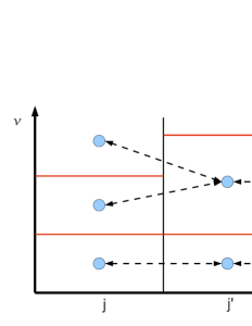
Figure 1.— Leakage probabilities can be thought of as weights ascribed to edges on a set of topologically distinct graphs in phase space. The vertical and horizontal axes represent frequency and spatial cell index, respectively. The horizontal in-cell partitions represent cell-specific frequency groupings. The shaded circles represent possible cell-group locations a DDMC particle or IMC particle may have and the dashed lines represent possible cell-group leakages at cell interfaces.

In Fig. 1, group bounds are given by horizontal lines at different values along the vertical frequency axis and cells are enumerated along the horizontal axis. The circles are possible $(j,g)$ locations of IMC-DDMC particles and the dashed lines represent transition possibilities for particles at those phase space locations. If all group bounds are aligned, the method reduces in complexity to the standard multigroup approach and the set of $(j,g)$-transition graphs become completely reducible. If a leakage is sampled, the probability of a DDMC to DDMC leakage transition is $(b_{j,g\leftrightarrow g_{D}^{\prime},n}\sigma_{j\rightarrow j^{\prime},g})/(b_{j,g,n}\tilde{\sigma}_{j\rightarrow j^{\prime},g})$ and the probability of an DDMC to IMC leakage transition is $(b_{j,g\leftrightarrow g_{T}^{\prime},n}\sigma_{b(j,j^{\prime}),g})/(b_{j,g,n}\tilde{\sigma}_{j\rightarrow j^{\prime},g})$. So the transition values for DDMC are these probabilities that sum to 1 for each $(j,g)$ DDMC region. If $(j,g)$ is treated with IMC, then the group in the subsequent cell is determined by particle frequency in the comoving frame of the boundary.

The fully hybridized comoving DDMC equation with elastic physical scattering is

$$\frac{1}{c}\frac{\partial\phi_{0,j,g}}{\partial t}+\bigg{(}\sum_{j^{\prime}}\tilde{\sigma}_{j\rightarrow j^{\prime},g}+(1-\gamma_{j,g,n})(1-f_{j,n})\sigma_{a,j,g,n}\\ +f_{j,n}\sigma_{a,j,g,n}\bigg{)}\phi_{0,j,g}=f_{j,n}\gamma_{j,g,n}\sigma_{P,j,n}acT_{j,n}^{4}\\ +\frac{1}{V_{j}}\sum_{j^{\prime}}V_{j^{\prime}}\sum_{g_{D}^{\prime}}\frac{b_{j,g\leftrightarrow g_{D}^{\prime},n}}{b_{j,g,n}}\sigma_{j^{\prime}\rightarrow j,g_{D}^{\prime}}\phi_{0,j,g_{D}^{\prime}}\\ +\frac{1}{V_{j}}\sum_{j^{\prime}}\sum_{g_{T}^{\prime}}\int_{A_{b(j,j^{\prime})}}\int_{\hat{\Omega}_{0}\cdot\vec{n}<0}\int_{g\leftrightarrow g_{T}^{\prime}}\ldots\\ P_{b(j,j^{\prime})}(|\hat{\Omega}_{0}\cdot\vec{n}|)|\hat{\Omega}_{0}\cdot\vec{n}|I_{0,\nu_{0}}d\nu_{0}d\Omega_{0}d^{2}\vec{r}\\ +\frac{\gamma_{j,g,n}(1-f_{j,n})}{V_{j}}\ldots\\ \sum_{g_{T}}\int_{V_{j}}\int_{4\pi}\int_{\nu_{g_{T}+1/2}}^{\nu_{g_{T}-1/2}}\sigma_{a,j,n}I_{0,\nu_{0}}d\nu_{0}d\Omega_{0}d^{3}\vec{r}\\ +\gamma_{j,g,n}(1-f_{j,n})\sum_{g_{D}}\sigma_{a,j,g_{D},n}\phi_{0,j,g_{D}}$$ (70)

where

$$\int_{g\leftrightarrow g^{\prime}}f(\nu)d\nu=\\ \begin{cases}\displaystyle\int_{\min([\nu_{g+1/2},\nu_{g-1/2}]\cap[\nu_{g^{\prime}+1/2},\nu_{g^{\prime}-1/2}])}^{\max([\nu_{g+1/2},\nu_{g-1/2}]\cap[\nu_{g^{\prime}+1/2},\nu_{g^{\prime}-1/2}])}f(\nu)d\nu\;\;,\\ \;\;[\nu_{g+1/2},\nu_{g-1/2}]\cap[\nu_{g^{\prime}+1/2},\nu_{g^{\prime}-1/2}]\not=\emptyset\\ \\ 0\;\;,\;\;[\nu_{g+1/2},\nu_{g-1/2}]\cap[\nu_{g^{\prime}+1/2},\nu_{g^{\prime}-1/2}]=\emptyset\;\;.\end{cases}$$ (71)

Groups represented by sub-indices $g_{D}$ or $g_{T}$ can be thought of as the complimentary sets over frequency that are used during the advance of particles. In other words, an optimization over frequency may be applied such that the comoving group structure in a time step is distinct from the user-prescribed group structure. This re-grouping must not degrade the accuracy of the observables of interest (for instance, a spectral tally of particles leaving the domain). Densmore’s approach to multifrequency DDMC lumps adjacent groups into a grey DDMC group (Densmore et al., 2012). Indices $(j,g)$ and $(j,g+1)$ are combined if their opacities multiplied by a characteristic cell length are greater than a threshold number of mean free paths per cell (Densmore et al., 2012; Abdikamalov et al., 2012). Additionally, this combined group has distinct Planck and Rosseland opacities,

$$\sigma_{P,j,g\cup g+1,n}=\frac{b_{j,g,n}\sigma_{a,j,g,n}+b_{j,g+1,n}\sigma_{a,j,g+1,n}}{b_{j,g,n}+b_{j,g+1,n}}\;\;,$$ (72)

and

$$\frac{1}{\sigma_{R,j,g\cup g+1,n}}=\frac{b_{j,g,n}/\sigma_{a,j,g,n}+b_{j,g+1,n}/\sigma_{a,j,g+1,n}}{b_{j,g,n}+b_{j,g+1,n}}\;\;,$$ (73)

respectively, where $g\cup g+1$ denotes a DDMC group union. Equations (72) and (73) can be used in place of $\sigma_{a,j,g,n}$ in the formulas for leakage opacity and in absorption sampling. The increase in efficiency is obtained from

$$\gamma_{j,g\cup g+1,n}=\gamma_{j,g,n}+\gamma_{j,g+1,n}\;\;.$$ (74)

For either $g$ or $g^{\prime}$, $\gamma_{j,g\cup g+1,n}$ used in the DDMC effective out-scattering coefficient, $(1-f_{j,n})(1-\gamma_{j,g\cup g+1,n})$, in place of the values on the left-hand-side of Eq. (74). For Densmore’s simulations (Densmore et al., 2012), only opacities that are monotonic in frequency are considered, so the group lumping method is conflated with a threshold frequency. Nothing in Densmore’s asymptotic analysis suggests that group lumping cannot be employed in frequency regions away from $\nu=0$. Densmore indeed notes the possibility of this extension (Densmore et al., 2012).

3. Code Verifications

In the numerical verification results that follow, we do not apply group lumping or irreducible group graphs (see Fig. 1), because applying these generalizations should not significantly reduce computation time, given the simple high-contrast opacity structures we use. For the plot legends, “HMC” stands for hybrid Monte Carlo and denotes instances of the method where both DDMC and IMC play a significant role. For simulations involving all or mostly DDMC, the plot label is “DDMC”. Otherwise, “IMC” is the label applied to computations that are transport dominant or constrained to only use IMC (referred to as pure IMC in captions).

3.1. Static Grid Verification

Our first verification is in a static material with a multifrequency structure that is amenable to analytic solution. Specifically, we use the Su & Olson (1999) picket fence opacity structure. We apply this picket fence opacity distribution to the static P₁ equations with thermal coupling. McClarren et al. (2008a) have solved the thermally coupled P₁ equations in grey materials for several one-dimensional geometries. The P₁ method is higher order than diffusion, but still approximate. This verification is therefore performed in an optically thick material where DDMC, IMC, and P₁ should show quantitative agreement for a range of spatial grids.

The picket fence opacity dependence on frequency can be constructed as the limit of a discrete multigroup distribution. Partitioning the frequency grid into regular $\Delta\nu$ intervals, a portion $p_{1}$ of $\Delta\nu$ is attributed an opacity $\sigma_{1}$ while the remainder $p_{2}=1-p_{1}$ is attributed an opacity $\sigma_{2}$. The limit as $\Delta\nu\rightarrow 0$ of this alternating grouping is the picket fence opacity $\sigma(\nu)$. Each picket at some $\nu$ is dense over the real number line of $\nu$; meaning both picket values are in any nonempty, open interval over the real number line for $\nu$.

The picket-fence distribution has the nice property that integrals of $I_{\nu}$ and $B_{\nu}$ over the dense groupings simplify when these integrands are assumed to be smooth (Su & Olson, 1999). Su and Olson solve the transport equations with the picket fence opacity to obtain a semi-analytic result. For specific values of $\sigma_{1}$, $p_{1}$, $\sigma_{2}$, and $p_{2}$, we may develop a simple generalization of McClarren’s P₁ solution that includes a rudimentary test of multifrequency for SuperNu.

Neglecting scattering, taking the zeroth and first angular moments of Eq. (1), and integrating the result over the set of frequencies that only yield a contribution from picket $g\in\{1,2\}$, the thermal picket fence P₁ equations in planar 1D geometry are

$$\frac{1}{c}\left(\frac{\partial E_{g}}{\partial t}+\frac{\partial F_{g}}{\partial z}\right)=\sigma_{g}(p_{g}aT^{4}-E_{g})+p_{g}S\;\;,$$ (75)

$$\frac{1}{c}\frac{\partial F_{g}}{\partial t}+\frac{c}{3}\frac{\partial E_{g}}{\partial z}=-\sigma_{g}F_{g}\;\;,$$ (76)

$$\frac{C_{v}(T)}{c}\frac{\partial T}{\partial t}=\sum_{g^{\prime}=1}^{2}\sigma_{g}E_{g}-\bar{\sigma}aT^{4}$$ (77)

where $z$ is the spatial coordinate, $E_{g}=\phi_{g}/c$ is the radiation energy density, $\bar{\sigma}=p_{1}\sigma_{1}+p_{2}\sigma_{2}$ and $S$ is an external source. The system of equations is linearized with $C_{v}(T)=a^{\prime}T^{3}$ (McClarren et al., 2008a; Su & Olson, 1999). Furthermore, we apply the usual non-dimensionalizations for convenience (McClarren et al., 2008a; Su & Olson, 1999):

$$x=\bar{\sigma}z\;\;,\;\;\epsilon=\frac{4a}{a^{\prime}}\;\;,\;\;\tau=\epsilon c\bar{\sigma}t\;\;,\;\;w_{g}=\frac{\sigma_{g}}{\bar{\sigma}}$$ (78)

and

$$\mathcal{E}_{g}=\frac{E_{g}}{aT_{r}^{4}}\;\;,\;\;\mathcal{F}_{g}=\frac{F_{g}}{aT_{r}^{4}}\;\;,\;\;\mathcal{M}=\frac{T^{4}}{T_{r}^{4}}\;\;,\;\;Q=\frac{S}{\bar{\sigma}aT_{r}^{4}}$$ (79)

where $T_{r}$ is a reference temperature. Incorporating Eqs. (78) and (79), Eqs. (75), (76) and (77) become

$$\epsilon\frac{\partial\mathcal{E}_{g}}{\partial\tau}+\frac{1}{c}\frac{\partial\mathcal{F}_{g}}{\partial x}=w_{g}(p_{g}\mathcal{M}-\mathcal{E}_{g})+p_{g}Q\;\;,$$ (80)

$$\epsilon\frac{\partial\mathcal{F}_{g}}{\partial\tau}+\frac{c}{3}\frac{\partial\mathcal{E}_{g}}{\partial x}=-w_{g}\mathcal{F}_{g}\;\;,$$ (81)

$$\frac{\partial\mathcal{M}}{\partial\tau}=\sum_{g^{\prime}=1}^{2}w_{g}\mathcal{E}_{g}-\mathcal{M}\;\;.$$ (82)

If Eqs. (80), (81), and (82) are Laplace transformed over time and reduced to equations for only energy density, what results are two fourth order linear differential equations in space with coefficients that are algebraically irrational functions of the Laplace variable, $s$. Denoting transformed quantities with a tilde, the equations can be solved to obtain $\tilde{\mathcal{E}}_{g}(x,s)$ and subsequently inverse Laplace-transformed to $\mathcal{E}_{g}$. The inverse Laplace transform of $\tilde{\mathcal{E}}_{g}$ is not known analytically, but it may be performed numerically. The material temperature is then proportional to a temporal convolution of the opacity weighted sum of the radiation energy densities, $\mathcal{E}_{g}$, and $e^{-\tau}$ (McClarren et al., 2008a).

To leverage the work done by McClarren, we constrain the $g=1$ picket with $w_{1}/w_{2}\ll 1$ or $w_{1}\approx 0$. The $g=2$ picket opacity is constrained to $w_{2}=\epsilon$. The relation between the non-dimensional optically thick picket and the non-dimensional heat capacity does not have physical justification but is merely a device to make certain expressions Laplace invertible. With $p_{2}w_{2}\approx 1$, $p_{2}\approx 1/\epsilon$ and $p_{1}\approx 1-1/\epsilon$, the value of $p_{1}$ can be comparable to $p_{2}$ despite the disparity in opacity strength. To our knowledge, the approach of relating $w_{2}$ with $\epsilon$ is novel.

With the above constraints and $Q=\delta(x)\delta(\tau)$, the Fourier-Laplace transformed system of equations is

$$(k^{2}+3\epsilon^{2}s^{2})\tilde{\tilde{\mathcal{E}}}_{1}=3\epsilon s\left(1-\frac{1}{\epsilon}\right)\;\;,$$ (83)

$$(k^{2}+3\epsilon^{2}s(s+2))\tilde{\tilde{\mathcal{E}}}_{2}=3(s+1)\;\;,$$ (84)

$$(s+1)\tilde{\tilde{\mathcal{M}}}\approx w_{2}\tilde{\tilde{\mathcal{E}}}_{2}\;\;,$$ (85)

where double tilde indicates a Fourier-Laplace transformed quantity. The remainder of the derivation follows closely from McClarren et al. (2008a) and is not repeated here. Solving the above equations yields the following kernel planar solutions for the constrained picket fence distribution:

$$\mathcal{E}_{1}=\left(1-\frac{1}{\epsilon}\right)\frac{\sqrt{3}}{2}\delta(\tau-\epsilon\sqrt{3}|x|)\;\;,$$ (86)

$$\mathcal{E}_{2}=\frac{1}{\epsilon}\frac{\sqrt{3}}{2}e^{-\tau}\Bigg{[}\frac{\tau I_{1}(\sqrt{\tau^{2}-3\epsilon^{2}x^{2}})}{\sqrt{\tau^{2}-3\epsilon^{2}x^{2}}}\Theta(\tau-\epsilon\sqrt{3}|x|)+\\ I_{0}(\sqrt{\tau^{2}-3\epsilon^{2}x^{2}})\delta(\tau-\epsilon\sqrt{3}|x|)\Bigg{]}\;\;,$$ (87)

and

$$\mathcal{M}=\frac{\sqrt{3}}{2}e^{-\tau}I_{0}(\sqrt{\tau^{2}-3\epsilon^{2}x^{2}})\Theta(\tau-\epsilon\sqrt{3}|x|)$$ (88)

where $\Theta$ is the Heaviside function, and $I_{0}$ ($I_{1}$) is the 0-order (1-order) modified Bessel function. Setting $\epsilon=1$ yields McClarren’s result (McClarren et al., 2008a). The properties of the P₁ equations allow for the application of a simple planar to spherical Green’s function mapping (McClarren et al., 2008a),

$$G_{\text{point}}(r,\tau)=-\frac{1}{2\pi r}\left.\frac{\partial G_{\text{plane}}}{\partial x}\right|_{x=r}\;\;,\;\;r>0\;\;,$$ (89)

where $G_{\text{point}}$ and $G_{\text{plane}}$ are the Green functions for 1D spherically symmetric and 1D planar geometry, respectively. Since Eqs. (86), (87), and (88) were derived with a kernel source, $\mathcal{E}_{g}$ or $\mathcal{M}$ may be substituted into the right hand side of Eq. (89). The unitless spherically symmetric material temperature kernel is

$$\mathcal{M}(r,\tau)=\\ \frac{3\sqrt{3}}{4\pi}e^{-\tau}\epsilon^{2}\frac{I_{1}(\sqrt{\tau^{2}-3\epsilon^{2}r^{2}})}{\sqrt{\tau^{2}-3\epsilon^{2}r^{2}}}\Theta(\tau-\epsilon\sqrt{3}r)+\\ \frac{3}{4\pi}e^{-\tau}I_{0}(\sqrt{\tau^{2}-3\epsilon^{2}r^{2}})\epsilon\frac{\delta(\tau-\epsilon\sqrt{3}r)}{r}\;\;.$$ (90)

The picket fence opacity is simple to implement in IMC-DDMC. Giving the nature of our picket fence constraint, we do not need group lumping or non-uniform particle transition probabilities. In this case, $\sigma_{P,j,n}=\bar{\sigma}$, $\gamma_{j,g,n}=p_{g}\sigma_{g}/\bar{\sigma}=p_{g}w_{g}$, and $\sigma_{a,j,g,n}=\sigma_{P,j,g,n}=\sigma_{R,j,g,n}$. We experiment with $\epsilon=2$, 15 or 50 cells over a spherical domain of 100 mean free paths, 400,000 source particles per time step over 100 time steps from $\tau=300$ to $\tau=600$. An MC particle propagates with DDMC when there are greater than 3 mean free paths per the particle’s $(j,g)$ coordinate. In order to simulate a problem with an instantaneous point source, we initialize the material temperature using the analytic solution and instantiate the initial MC particle field accordingly. Figure 2 contains 15 cell IMC-DDMC material temperature data plotted against Eq. (90).

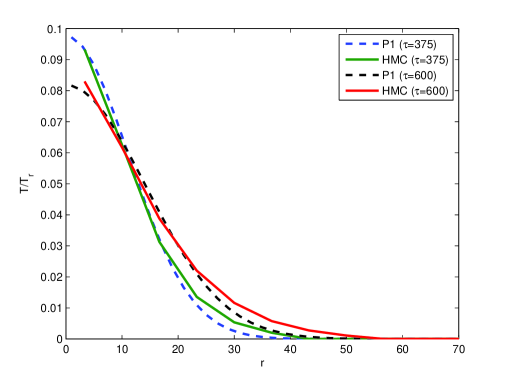
Figure 2.— P₁ (dashed) and IMC-DDMC (solid) unitless material temperature profiles at two different (mean free) times plotted as a function of unitless radius (mean free paths). These curves are solutions to the picket-fence opacity problem described in Section 3.1. At 6.67 mean free paths per spatial cell, only DDMC is applied to radiation interacting with the $g=2$ picket. For the $g=1$ picket, IMC allows the radiation to stream out of the domain and hence plays no role in the thermal state. The combined MC particle fields produce an accurate solution tally with respect to the analytic P₁ solution at coarse spatial resolution.

The 50 cell case should be more converged at each time relative to the results in Fig. 2. Indeed, in Fig. 3 we see that IMC is now applied everywhere in the spectrum and the solution is more converged.

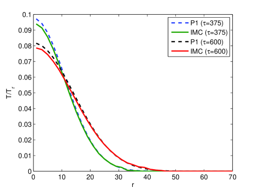
Figure 3.— P₁ (dashed) and IMC-DDMC (solid) unitless material temperature profiles at two different (mean free) times plotted as a function of unitless radius (mean free paths). These curves are solutions to the picket-fence opacity problem described in Section 3.1. At 2 mean free paths per spatial cell, only IMC is applied to both $g=1$ and $g=2$ radiation fields. Relative to the coarse grid solutions of Fig. (2), the IMC-DDMC solution tally is in closer agreement with the P₁ solutions.

We next measure the error of IMC and DDMC relative to the P₁ temperature solution for different numbers of spatial cells. A grid convergence study for a stochastic method must have enough particles per cell to make the statistical error negligible. Another consideration involves a peculiarity of IMC specifically. Much work in IMC pertaining to the effect of the spatial grid on the continuous transport has been to formally characterize a pathology referred to as teleportation error (McKinley et al., 2003; Densmore, 2011). Teleportation error occurs in IMC when there are many absorption mean free paths per cell but not many absorption mean free times per time step. Particle energies absorbed at one location in a cell may be re-emitted in a subsequent time step many mean free paths away from the absorption locations (McKinley et al., 2003). Densmore (2011) demonstrates formally that a piecewise constant representation of scalar flux along with a time step that resolves a mean free time does not asymptotically converge to a correct discretization of the diffusion equation.

Despite these complications, there does exist literature to indicate that the IMC temperature error scales with $\Delta r$ where $\Delta r$ is a typical cell size of the simulation (if not the actual cell length for a one dimensional simulation). In investigating a method to emit particles at sub-cell deposition locations, Irving et al. (2011) measure total relative error of standard IMC for a 1D Marshak wave problem in planar geometry to a converged solution at several temporal and spatial resolutions. While not explicitly stated, their findings appear to yield an total relative error of about $9/J$, particularly between $J=10$ and $J=30$ cells, for several time step sizes. Cheatham (2010) plots relative errors of IMC with respect to a grey form of the Su & Olson (1999) solutions in two cells of a simulation. This IMC error also appears to roughly scale linearly with cell width for each cell. Having set each simulation to have well over 13,000 particles generated per cell per time step and testing in a regime where IMC teleportation should be minimal, Fig. 4 indicates our code indeed achieves an approximately linear scaling in L₂ relative error for both IMC and DDMC as well.

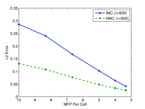
Figure 4.— IMC (solid) and IMC-DDMC (dashed) L₂ temperature error relative to the P₁ solution plotted over the number of mean free paths per cell at 600 mean free times. From 10 to 30 cells (10 to about 3.33 mean free paths per cell), IMC and DDMC appear to linearly converge. The error from IMC-DDMC (where DDMC contributes non-negligibly to the temperature) is found to be distinctively lower than that of pure IMC down to 3.33 mean free paths per cell.

Our results indicate that DDMC computes temperature with higher fidelity at low cell resolution for this particular problem. Having obtained good agreement with a static grid analytic solution, we present and test a manufactured solution the next section that allows for outflow and a group structure that includes scattering and absorption.

3.2. Manufactured Verification

The Method of Manufactured Solutions (MMS) (Oberkampf & Roy, 2010, p. 219) provides an avenue of code verification that is useful for problems with governing equations that are not amenable to a direct solution with a prescribed source. As the name MMS suggests, one postulates, or manufactures, a solution (McClarren et al., 2008b; Warsa & Densmore, 2010). The next step simply involves incorporating this postulated answer into the system of equations to see what additional terms are produced through calculus and algebra (McClarren et al., 2008b). The additional terms can be included in an appropriate code as artificial sources. If the routines in the code function and interface correctly, the numerical experiment should reproduce the manufactured solution. Manufactured solutions have been developed by Warsa & Densmore (2010) for discrete ordinate codes modeling diffusive problems and by McClarren et al. (2008b) for planar, grey radiation-hydrodynamics problems in the optically thick and optically thin limits. We draw from these solutions as well as analytic forms presented by (Mihalas & Mihalas, 1984, p. 474), and by Pinto & Eastman (2000) for high velocity outflow problems.

Our manufactured solution has two groups and the temperature and radiation fields are constant in time and over the space of the expansion. As will be shown, in order to achieve an ostensibly simple solution, the code must have a time dependent source that can be distinct in form for each group. The source must supply energy to counteract the non-trivial adiabatic cooling of the field. The higher energy group has pure elastic scattering and the remaining group has both elastic scattering and absorption. These groups must couple through Doppler shifting in a way that appropriately balances the supply of energy to each group. Moreover, the solutions must exhibit an invariance with respect to several wavelength or frequency grid values.

The constrained material properties are

$$\vec{U}(r,t)=\frac{U_{\max}\vec{r}}{R(t)}\;\;,$$ (91a)

$$\rho(r,t)=\rho(t)=\frac{3M}{4\pi R(t)^{3}}\;\;,$$ (91b)

where $\vec{U}(r,t)$ is fluid velocity, $\rho(r,t)$ is density, $U_{\max}$ is the maximum outflow speed, $R(t)=R(0)+U_{\max}t$ is the outer expansion radius, $\vec{r}$ is the Eulerian position vector, and $M$ is the total outflow mass. The frequency integrated manufactured radiation intensity and temperature are

$$I_{0}(r,t)=\frac{\phi_{m}}{4\pi}\;\;,$$ (92a)

$$T(r,t)=T_{m}=(\phi_{m}/(ca))^{1/4}\;\;,$$ (92b)

respectively. The subscript $m$ denotes a manufactured value. For a general frequency grid, $\nu_{G+1/2}<\nu_{G-1/2}<\ldots<\nu_{1/2}$, and group index, $g\in\{1\ldots G\}$, we constrain the absorption opacity to be pre-grouped as

$$\sigma_{0,\nu_{0},a}=\sigma_{g}(t)=\kappa_{g}\rho(t)\;\;,$$ (93)

where $\kappa_{g}$ is constant within group $g$. The differential scattering opacity has the form

$$\sigma_{0,s}(\nu_{0}^{\prime}\rightarrow\nu_{0},\hat{\Omega}_{0}^{\prime}\cdot\hat{\Omega}_{0})=\frac{\sigma_{s}(t)}{4\pi}\delta(\nu_{0}^{\prime}-\nu_{0})=\rho(t)\frac{\kappa_{s}}{4\pi}\delta(\nu_{0}^{\prime}-\nu_{0})\;\;,$$ (94)

where $\kappa_{s}$ is a constant. We now may express the manufactured multifrequency solution as an opacity-dependent superposition of the normalized Planck function and a piecewise constant function,

$$\varphi_{m,\nu_{0}}=\left(\frac{\sigma_{s}}{\sigma_{g}+\sigma_{s}}\right)\frac{\varphi_{m,s,g}}{\Delta\nu_{g}}+\left(\frac{\sigma_{g}}{\sigma_{g}+\sigma_{s}}\right)b_{\nu_{0}}\;\;,\\ \nu_{0}\in[\nu_{g+1/2},\nu_{g-1/2}]\;\;,$$ (95)

where $I_{0,\nu_{0}}=I_{0}\varphi_{m,\nu_{0}}$, $\varphi_{m,s,g}$ is the uniform non-thermal contribution to $g$ and $b_{\nu_{0}}$ is the normalized Planck function. With particular choices of opacity, frequency grid, and $\varphi_{m,s,g}$, the integral of $\varphi_{\nu_{0}}$ may be constrained to 1.

Incorporating the form of the opacities into the transport and temperature equations, the system to be solved with manufactured sources is

$$\left(1+\hat{\Omega}_{0}\cdot\frac{\vec{U}}{c}\right)\frac{1}{c}\frac{DI_{0,\nu_{0}}}{Dt}+\hat{\Omega}_{0}\cdot\nabla I_{0,\nu_{0}}-\frac{1}{c}\hat{\Omega}_{0}\cdot\nabla\vec{U}\cdot\hat{\Omega}_{0}\nu_{0}\frac{\partial I_{0,\nu_{0}}}{\partial\nu_{0}}\\ -\frac{1}{c}\hat{\Omega}_{0}\cdot\nabla\vec{U}\cdot(\mathbf{I}-\hat{\Omega}_{0}\hat{\Omega}_{0})\cdot\nabla_{\hat{\Omega}_{0}}I_{0,\nu_{0}}+\\ \frac{3}{c}\hat{\Omega}_{0}\cdot\nabla\vec{U}\cdot\hat{\Omega}_{0}I_{0,\nu_{0}}=\frac{1}{4\pi}\sigma_{g}b_{\nu_{0}}(T)acT^{4}-(\sigma_{g}+\sigma_{s})I_{0,\nu_{0}}\\ +\frac{\sigma_{s}}{4\pi}\int_{4\pi}I_{0,\nu_{0}}(\vec{r},\hat{\Omega}_{0}^{\prime},t)d\Omega_{0}^{\prime}+\frac{S_{m,\phi,\nu_{0}}(r,t)}{4\pi}\;\;,$$ (96)

and

$$C_{v}\frac{DT}{Dt}=\\ \sum_{g=1}^{G}\int_{4\pi}\int_{\nu_{g+1/2}}^{\nu_{g-1/2}}\sigma_{g}(I_{0,\nu_{0}}-acT^{4}b_{0,\nu_{0}})d\nu_{0}d\Omega_{0}\\ +S_{m,T}(r,t)\;\;,$$ (97)

where $S_{m,\phi,\nu_{0}}$ and $S_{m,T}$ are the manufactured radiation and material sources to be determined. At implementation, $S_{m,T}$ can be treated with the usual Fleck factor re-balance of material source terms. With the manufactured solutions specified, the source terms are found to be

$$\frac{S_{m,\phi,\nu_{0}}}{\phi_{m}}=\frac{U_{\max}}{cR(t)}\left(3\varphi_{m,\nu_{0}}-\nu_{0}\frac{\partial\varphi_{m,\nu_{0}}}{\partial\nu_{0}}\right)\\ +\sigma_{g}(\varphi_{m,\nu_{0}}-b_{\nu_{0}}(T_{m}))\;\;,$$ (98)

and

$$\frac{S_{m,T}}{\phi_{m}}=\sum_{g=1}^{G}\sigma_{g}(b_{g}(T_{m})-\varphi_{m,g})\;\;,$$ (99)

where $\varphi_{m,g}=\int_{\nu_{g+1/2}}^{\nu_{g-1/2}}\varphi_{m,\nu_{0}}d\nu_{0}$. Integration of Eq. (98) over group $g$ yields

$$\frac{S_{m,\phi,g}}{\phi_{m}}=\\ \frac{U_{\max}}{cR(t)}\left(4\varphi_{m,g}-\nu_{g-1/2}\varphi_{m,\nu_{g-1/2}}+\nu_{g+1/2}\varphi_{m,\nu_{g+1/2}}\right)\\ +\sigma_{g}(\varphi_{m,g}-b_{g}(T_{m}))$$ (100)

We now construct a two group instantiation of Eqs. (99) and (100) that is simple to implement but is a good test of energy balance and group coupling in the code. A scattering opacity $\sigma_{s}=0.1\rho(t)$ is applied along with absorption opacities $\sigma_{1}=0$ and $\sigma_{2}=0.1\rho(t)$. The sub-group profile of the radiation energy density in $g=1$ is constant. Thus, particle frequency may be sampled uniformly in $g=1$. If the group domains are implemented in wavelength, then the MC source particle wavelengths in $g=1$ must be calculated as the reciprocal of a uniform sampling between the reciprocals of the group wavelength bounds. Since radiation only redshifts, the upwind group approximation (Mihalas & Mihalas, 1984, p. 475) for the group-interface terms in Eq. (100) must be a reasonable approach for Eq. (95) and the MC process described. Equation (100) consequently may be expressed as

$$\frac{S_{m,\phi,1}}{\phi_{m}}=\frac{U_{\max}}{cR(t)}\left(4\varphi_{m,1}+\nu_{3/2}\varphi_{m,\nu_{3/2}}^{+}\right)\;\;,$$ (101)

and

$$\frac{S_{m,\phi,2}}{\phi_{m}}=\frac{U_{\max}}{cR(t)}\left(4\varphi_{m,2}-\nu_{3/2}\varphi_{m,\nu_{3/2}}^{+}\right)+\\ \sigma_{2}(\varphi_{m,2}-b_{2}(T_{m}))\;\;,$$ (102)

where the plus superscript denotes evaluation on the right side of the frequency bound. We exploit our ability to choose a frequency grid that further simplifies the form of the source terms. Using Eq. (95), if $\nu_{5/2}=0$, $\varphi_{m,s,1}=\varphi_{m,s,2}=1/2$ and the integral of $b_{\nu_{0}}$ over $\nu_{0}\in[0,\nu_{3/2}]$ is 1/2, then $\varphi_{2}=b_{2}=1/2$ and the source terms become

$$\frac{S_{m,\phi,1}}{\phi_{m}}=\frac{U_{\max}}{cR(t)}\left(2+\frac{1}{2}\frac{\nu_{3/2}}{\Delta\nu_{1}}\right)\;\;,$$ (103)

$$\frac{S_{m,\phi,2}}{\phi_{m}}=\frac{U_{\max}}{cR(t)}\left(2-\frac{1}{2}\frac{\nu_{3/2}}{\Delta\nu_{1}}\right)\;\;,$$ (104)

and

$$S_{m,T}=0$$ (105)

Newton iteration yields $h\nu_{3/2}/kT_{m}\approx 3.503$ to obtain $b_{2}(T_{m})=1/2$. To satisfy Eq. (105), the MC process must deposit the correct energy in $g=2$ directly from radiation generated in $g=2$ and indirectly from redshifting radiation originating in $g=1$. The strength of the group coupling is quantified with $\nu_{3,2}/\Delta\nu_{1}$.

The numerical results for our manufactured solution include strong and weak Doppler coupling for pure IMC, IMC-DDMC, and pure DDMC. For the IMC-DDMC hybrid, IMC is employed in the pure scattering group and DDMC is employed in the thermally coupled group. We note there are several ways to implement the Doppler shifting in the pure DDMC test that are equivalent. For instance, the group bound terms on the right-hand-side of Eq. (30) can be implemented with the upwind approximation as probabilities of redshift during the DDMC process if the scattering is elastic. For the following results, each DDMC particle has its wavelength or frequency sampled according to the sub-group distribution (which is constant in this case) after transport. The frequency value is redshifted by the same formula that lowers the particle’s energy weight. If the new value of frequency is located in a new group, the particle is transferred to that group for the next time step.

For the first test, we set $\nu_{3/2}/\Delta\nu_{1}\approx 0.036$ which of course is small relative to 4. The other domain quantities are set in a manner that makes adiabatic cooling of the trapped radiation field non-negligible: $U_{\max}=10^{9}$ cm/s, $R(0)=1.728\times 10^{14}$ cm, $t\in[172,800,181,440]$ seconds (or 2 to 2.1 days), $M=10^{33}$ g, $C_{v}=2\times 10^{7}\rho$, $T_{m}=1.1602\times 10^{7}$ K, and a wavelength grid of $\{\lambda_{1/2},\lambda_{3/2},\lambda_{5/2}\}=\{1.239\times 10^{-9},3.542\times 10^{-8},1.2398\times 10^{-3}\}$ cm.

The pertinent computational quantities are: 10 time steps, $J=10$ spatial cells, 400,000 source particles generated per time step, 400,000 initial particles. For the specification provided, we expect the code to produce reasonable agreement to the manufactured profiles. Figures 5a and 5b have pure IMC data for radiation energy density and temperature at several times, respectively.

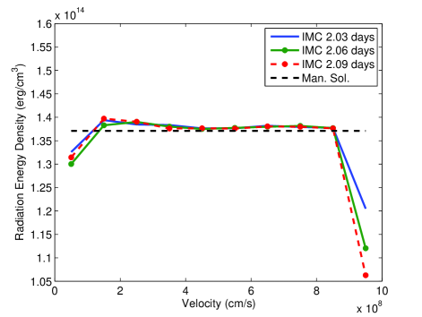
(a)

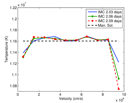
(b)

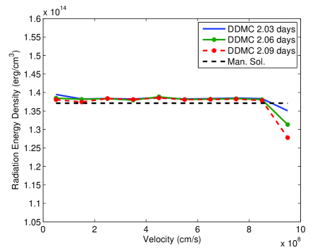
(c)

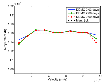
(d)

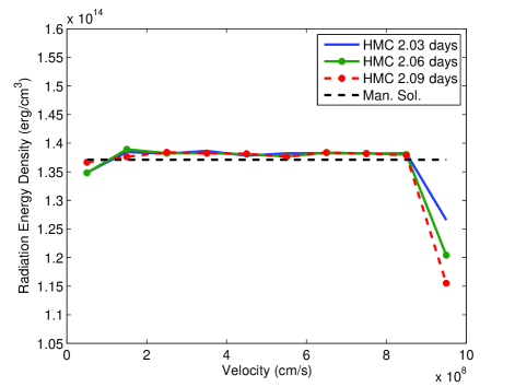
(e)

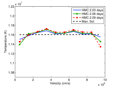
(f)

Figure 5.— Manufactured (dashed) and simulated radiation energy densities (left figures) and temperatures (right figures) at three different times (solid, dot-solid, and dot-dashed). Figures 5a and 5b have IMC, Figs. 5c and 5d have DDMC, and Figs. 5e and 5f have IMC-DDMC. These MC profiles are generated by implementing the manufactured source described in Section 3.2. Specifically, data in Figs. 5a, 5b, 5c, and 5d use a wavelength grid that admits a weak Doppler coupling between the groups while data in Figs. 5e and 5f use a wavelength grid that admits a strong Doppler coupling between the groups. The IMC deviation from uniformity towards the origin is apparently due to statistical noise and can be reduced by increasing the number of source or initial particles allocated per cell. The deviation at the outer bound is due to radiation escaping into an adjacent vacuum. This test verifies that the code reproduces the analytic solution in each of the modes of operation: IMC, DDMC and IMC-DDMC.

Figures 5c and 5d have pure DDMC data for radiation energy density and temperature at several times, respectively. The DDMC results indicate the method does not predict as much leakage at the outer cell as IMC through the observed times. DDMC appears to produce less noise near the origin for the problem depicted.

We do not show the IMC-DDMC results for this problem here but note that they too reproduce the manufactured profiles over the computed time scale. With the computation time of pure DDMC scaled to 1, the following table has the relative computation times of IMC-DDMC and IMC for the weak coupling manufactured source test.

Table 1Weak Group Coupling Computation Times

Method	Scaled Time
DDMC	1
HMC	27.25
IMC	147.39

We now change the coupling term to be comparable to 4 with a value of $\nu_{3/2}/\Delta\nu_{1}\approx 3.0$. This is a more strenuous test on the code’s ability to tally the correct redshift rates because the manufactured source in $g=2$ is much reduced. The modified wavelength grid has $\lambda_{1/2}=2.656838745\times 10^{-8}$ cm to implement this coupling strength. Otherwise, all quantities are the same from the weak coupling test. The IMC-DDMC radiation energy density and temperature results for this test are shown in Fig. 5e and 5f. Results for pure IMC and pure DDMC are similar.

The DDMC scaled computation times for the strong redshift coupling test are tabulated below.

Table 2Strong Group Coupling Computation Times

Method	Scaled Time
DDMC	1
HMC	44.89
IMC	110.39

We ensure the pure scattering group, $g=1$, indirectly sustains the temperature profile’s steady state by removing the radiation in that group. The profile should steadily drop relative to the solution that includes Doppler shifting. Evidence for this effect can be found in Figs. 6a and 6b.

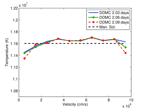
(a)

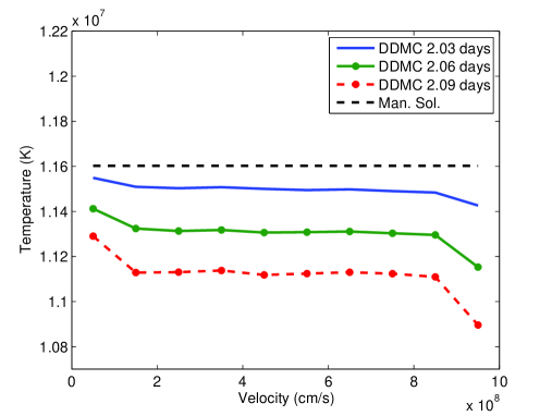
(b)

Figure 6.— Manufactured (dashed) and DDMC (solid, dot-solid, and dot-dashed) material temperature at three different times plotted over the velocity grid. The MC profiles in Fig. 6a are generated by implementing the manufactured source described in Section 3.2 with strong between-group redshift coupling. It is evident that a steady state is maintained at the inner regions of the domain. The MC profiles is Fig. 6b are generated in nearly the same manner but leave the lower wavelength ($g=1$) group sourceless. In Fig. 6b, the non-equilibrium in temperature is a result of the higher wavelength ($g=2$) group not being able to produce a steady state temperature without an additional source of Doppler shifted radiation (from $g=1$). The purely elastic scattering $g=1$ group thus has an indirect yet important effect on the temperature for the strong Doppler coupling described.

3.3. Spherical Heaviside Source Tests

Finally, we construct a multigroup outflow problem that may be used to test both code efficiency and quality of the operator split treatment of grid motion in IMC-DDMC. The problem consists of a Heaviside spherical source out to $0.8U_{\max}$ of strength 4$\times 10^{24}/(t_{n}+t_{\min})^{3}$ ergs/cm³/s in a purely absorbing fluid. The opacity is over 10 groups logarithmically spaced in wavelength from 1.238$\times 10^{-9}$ cm to 1.238$\times 10^{-3}$ cm. As in the manufactured solution, we alternate small and large opacities across the wavelength grouping where odd groups have the larger opacity. Again, the speed $U_{\max}=10^{9}$ cm/s and the total mass $M=10^{33}$ g. Instead of equal density in each cell, we attribute $M/J$ mass to each cell for $J$ fluid cells. Uniformly partitioning the mass creates a density gradient that couples into the transport process through the macroscopic opacity. All simulations in this section use 50 velocity cells from 0 cm/s to $U_{\max}$, 192 time steps from 2 days to 11 days, and 100,000 source particles per time step. The heat capacity is adopted from Pinto & Eastman (2000); $C_{v}\approx 2\times 10^{7}\rho$ ergs/cm³/K. For the calculations discussed, we use DDMC for cell $j$ when $\Delta U_{j}\Delta t_{n}\sigma_{g}\geq\tau_{\text{DDMC}}$ and IMC otherwise. Following Abdikamalov et al. (2012), we have labeled the threshold mean free path number between IMC and DDMC as $\tau_{\text{DDMC}}$. For the first two tests discussed, depicted in Figs. 7a and 8, $\tau_{\text{DDMC}}=3$. For the tests of the new boundary condition, depicted in Figs. 7b and 9, $\tau_{\text{DDMC}}=3$ for Fig. 7b and $\tau_{\text{DDMC}}=10$ for Fig. 9. As a consequence of the problem’s structure, the density gradient creates a “method front” for IMC-DDMC where an outer shell of IMC moves inward over the grid. The method front is heterogeneous in group space, meaning the even groups are converted to IMC sooner (or are already IMC) over the specified problem duration.

The discrepancies between the IMC and IMC-DDMC profiles in Figs. 7a and 8 arise in part from implementing Eq. (33) instead of Eq. (61). For mean free path thresholds on the order of 2 to 3 per cell, we find that these errors are systematic yet generally minimal. The discrepancy can be made much worse by implementing a more conservative mean free path threshold of about 10 for this problem set. Higher mean free path thresholds require IMC particles emitted from a DDMC spatial surface to propagate through an optically thicker sub-cell environment. Of course this discrete interface is not present for pure IMC; in other words there is not a significant source of IMC radiation originating from one surface in pure IMC since the method interface is not present. Complementarily, the DDMC field is not as sourced by IMC radiation for a high mean free path threshold. This is discernible from the form of $P_{b(j,j^{\prime})}(\mu)$. We demonstrate that incorporating an approximation of the new factor, $G_{U}$, from Eq. (61) indeed appears to mitigate the over-redshift near the method front in Figs. 7b and 9. However, we recommend a mean free path threshold in the range of 2 to 5 mean free paths. Arguments presented by Pinto & Eastman (2000) indicate that diffusion theory remains valid on large outflow time scales if radiation momentum does not greatly affect fluid momentum.

In the first case tested, we use

$$\sigma_{g}=\begin{cases}0.13\rho\;\;,\;\;g=2k-1\\ 0.13\times 10^{-4}\rho\;\;,\;\;g=2k\;\;.\end{cases}$$ (106)

Results for Eq. (106) are plotted in Fig. 7a. We find IMC-DDMC is faster than IMC by a factor of 3.36.

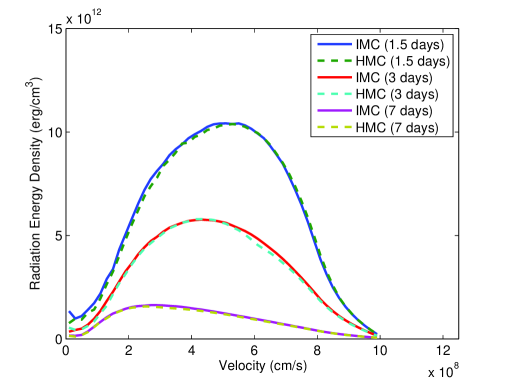
(a)

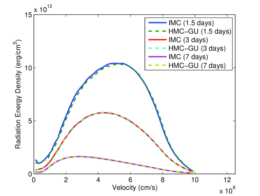
(b)

Figure 7.— Radiation energy density for pure IMC (solid lines) and IMC-DDMC (dashed lines) at three times for an expanding domain with a $4\times 10^{24}/(t_{n}+t_{\min})^{3}$ erg/cm³/s spherical Heaviside source from the expansion center out to the location of the fluid moving at $8\times 10^{8}$ cm/s. The opacity is defined over 10 logarithmic wavelength groups with a magnitude of $0.13\rho$ cm^-1 in odd groups and $0.13\times 10^{-4}\rho$ cm^-1 in even ($\rho$ is density in g/cm³). Because equal mass is attributed to each of the fifty fluid cells, the density is not radially uniform. At day 1.5, most particles are propagating with DDMC. By day 7, most particles are propagating with IMC. For this problem, $\tau_{\text{DDMC}}=3$ and IMC-DDMC is faster than IMC by a factor of 3.36. In Fig. 7a, the standard IMC-DDMC boundary condition is used; at 3 and 7 days the boundary discrepancy has propagated to about $6\times 10^{8}$ cm/s and $4\times 10^{8}$ cm/s, respectively. In Fig. 7b, we have implemented the fit, Eq. (108) with $C_{1}=0.55$ and $C_{2}=1.25$, of the amplification factor, and find for this problem, with the IMC-DDMC threshold at 3 mean free paths, that the method boundary induced error has essentially been removed.

In the second case tested, we use

$$\sigma_{g}=\begin{cases}0.13\rho\;\;,\;\;g=2k-1\\ 0.13\times 10^{-7}\rho\;\;,\;\;g=2k\;\;.\end{cases}$$ (107)

Results for Eq. (107) are plotted in Fig. 8. We find IMC-DDMC is faster than IMC by a factor of 4.59. We have improved the performance of IMC-DDMC relative to IMC by increasing the disparity in adjacent group opacities. If instead the $g=2k-1$ opacities are increased, IMC-DDMC provides even further improvement in the diffusive groups of the spectrum. In both simulations, IMC-DDMC transitions to pure IMC over the 9 day period.

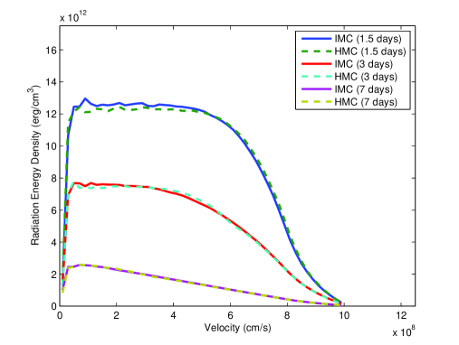
Figure 8.— Radiation energy density for pure IMC (solid lines) and IMC-DDMC (dashed lines) at three times for an expanding domain with a $4\times 10^{24}/(t_{n}+t_{\min})^{3}$ erg/cm³/s spherical Heaviside source from the expansion center out to the location of the fluid moving at $8\times 10^{8}$ cm/s. The opacity is defined over 10 logarithmic wavelength groups with a magnitude of $0.13\rho$ cm^-1 in odd groups and $0.13\times 10^{-7}\rho$ cm^-1 in even ($\rho$ is density in g/cm³). Because equal mass is attributed to each of the fifty fluid cells, the density is not radially uniform. At day 1.5, most particles are propagating with DDMC. By day 7, most particles are propagating with IMC. For this problem, IMC-DDMC is faster than IMC by a factor of 4.59.

We now describe a possible implementation of Eq. (61). There are two readily discernible means of ascribing a MC interpretation to the $G_{U}(\mu)$ factor. In one, the probability that an IMC particle transmits into DDMC when incident on a diffusive region may be taken as $P(\mu)\sim(1+3\mu/2)G_{U}(\mu)$. However, this would make $P(\mu)>1$ for some $\mu$ regardless of cell material properties. To constrain $P(\mu)\leq 1$, some range of angular projections, $\mu\in[0,\varepsilon]$, where $\varepsilon<1$, would have to have $G_{U}$ modified. As an alternative, the probability of IMC to DDMC transmission may be maintained as its original form $P(\mu)\sim 1+3\mu/2$ and the particle weight must then be multiplied by $G_{U}(\mu)$. Since $G_{U}(\mu)$ is of O($1/\mu$), the energy current across the IMC-DDMC interfaces is bounded. Physically, it is supposed that this implies the importance of IMC particles interacting with a surface at a DDMC region to the energy balance in the adjacent cells must still be bounded at small values of $\mu$. In our tests, for an inner DDMC region adjacent to an outer IMC region at a boundary with speed $U$,

$$G_{U}(\mu)=1+2\frac{U}{c}\left(\frac{C_{1}}{\mu}-C_{2}\mu\right)\;\;,$$ (108)

where $C_{1},C_{2}>0$ are constants. In passing, we note that a angularly uniform, heuristic $G_{U}$ may be calibrated from simulation. From phenomenological considerations, it is found that a good form of $G_{U}$ is

$$\bar{G}_{U}=1+2\min(0.055\tau_{\text{DDMC}},1)\frac{U}{c}$$ (109)

at least for a range of $\tau_{\text{DDMC}}\in[3,10]$. Applying Eq. (108) with $C_{1}=0.55$ and $C_{2}=1.25$ for $\tau_{\text{DDMC}}=\Delta U_{j}\Delta t_{n}\sigma_{g}=3$ and Eq. (106), we see a small improvement in Fig. 7b.

To further demonstrate the potential utility of Eq. (108), we apply the $G_{U}$ factor to a problem where the discrepancy is made very large by setting $\tau_{\text{DDMC}}=10$. The fitting constants for this test are $C_{1}=0.6$ and $C_{2}=1.25$. We observe a significant improvement at all times including when the discrepancy is very large at 1.5 days, as plotted in Fig. 9. However, with this improvement comes some additional MC noise due to the weight modifications having a large range of $G_{U}$ and insufficient sampling for $\mu\rightarrow 0$. Since the IMC portion of the simulation is in the lab frame, the minimal comoving projection into the DDMC interface cell is $U/c$. But physically, the comoving projection lower bound is 0. For sampling comoving directions with $\mu<U/c$, the new boundary condition is applied to particles with $\mu<U/c$ that are advected onto DDMC surfaces through the velocity position shift algorithm delineated in Section 2.4. We find that these samplings are not important for $\tau_{\text{DDMC}}=3$ but are important for $\tau_{\text{DDMC}}=10$ or greater. At larger $\tau_{\text{DDMC}}$, IMC particles that “graze” the DDMC surface are important due to the increased level of angular isotropy near the IMC-DDMC boundary. We note that the proper implementation of the weight modifying factor, $G_{U}$, is an open research question. Additionally, our choice of asymptotic scalings and analysis in Section 2.3 is approximate and tailored for homologous outflow.

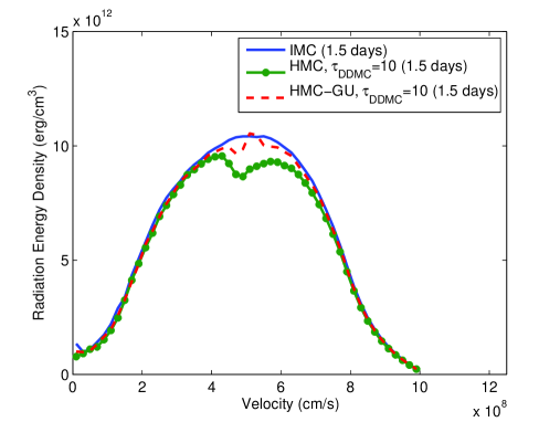
Figure 9.— Radiation energy density for pure IMC (solid line), IMC-DDMC without a $G_{U}$ factor (dotted solid line), and IMC-DDMC with Eq. (108) (dashed line) at 1.5 days after initial time with a $4\times 10^{24}/(t_{n}+t_{\min})^{3}$ erg/cm³/s spherical Heaviside source from the expansion center out to the location of the fluid moving at $8\times 10^{8}$ cm/s. The opacity is defined over 10 logarithmic wavelength groups with a magnitude of $0.13\rho$ cm^-1 in odd groups and $0.13\times 10^{-4}\rho$ cm^-1 in even ($\rho$ is density in g/cm³). The introduction of the $G_{U}$ factor into IMC-DDMC has improved agreement with pure IMC for $\tau_{\text{DDMC}}=10$, but error persists. Additionally, some Monte Carlo noise is added due to the large range of $G_{U}(\mu)$ modifying particle weights. To avoid this issues for the method described, we recommend a $\tau_{\text{DDMC}}$ threshold between 2 and 5.

We caution that what may be thought of as a conservative selection of a mean free path threshold between IMC and DDMC may lead to the types of errors depicted in Fig. 9.

4. Conclusions and Future Work

We have described an approach to multifrequency IMC-DDMC on a “velocity grid” that is semi-implicit, accelerated by diffusion theory, and relativistic to first order. Additionally, we have provided an algorithm for treating the operator split motion of Lagrangian grid boundaries that is simple to integrate into any IMC-DDMC scheme possessing hydrodynamic effects. This treatment of radiation transport is a viable candidate for simulating the post-explosion phase of thermonuclear supernovae.

In Sections 3.1 and 3.2, we have provided a simple generalization of McClarren’s analytic P₁ solutions (McClarren et al., 2008a) for static material multifrequency verification and a manufactured solution for multigroup outflow verification. We find that SuperNu produces good agreement with both analytic solutions.

In Section 3.3, we perform spherical Heaviside source simulations with high-disparity grouped opacities in the presence of a fluid density gradient. This density gradient induces a “method front” in IMC-DDMC where an inward moving region of pure IMC starting at the outermost fluid cell replaces DDMC in the optically thick groups. For our tests, IMC-DDMC produces good agreement with pure IMC at all method front locations over the velocity grid; this indicates that the Lagrangian grid boundary algorithm and the particular choice of mean-free-path based coupling between IMC and DDMC are functioning properly.

We have discovered that when the fluid velocity is semi-relativistic, an important correction term is necessary at IMC-DDMC boundaries. In our findings, we have seen that errors over 10% in radiation energy density may manifest in IMC-DDMC relative to pure IMC for reasonable input parameters if the standard IMC-DDMC boundary condition is used. The corrective term generally reduces these boundary errors and increases the viable range of IMC-DDMC mean-free-path thresholds. However, we note that the best results observed are for thresholds on the order of 2 to 5 mean free paths even with the new boundary condition. Despite the singularity in the new factor, the influence of all particles on the energy balance in each cell is finite by virtue of the analysis performed in Section 2.3. In Section 3.3, we have shown that these discrepancies may occur in astrophysical problems. Also in Section 3.3, we have used the modified IMC-DDMC boundary condition to indeed improve agreement between IMC-DDMC and pure IMC for different values of mean free path threshold, $\tau_{\text{DDMC}}$. We note that the theory and implementation of the corrective boundary factor presented here requires further exploration. These Heaviside tests additionally demonstrate that IMC-DDMC performs much better than pure IMC in terms of accuracy and speed when there are large disparities between the magnitudes of opacities in adjacent groups, which is the primary motivation of this work.

We plan to incorporate nonuniform frequency or wavelength groups across spatial cells (Densmore et al., 2012). In order to do so, fully general phase space leakage graphs must be implemented. These graphs (qualitatively depicted in Fig. 1) along with group lumping (Eqs. (72)-(74)) may help improve efficiency for transport problems with many groups and ill-behaved spectral properties. Additionally, we plan to further investigate alternative implementations of the theory presented in Section 2.3. The initial target application for the one dimensional, spherically symmetric code is Nomoto’s W7 model (Nomoto et al., 1984). We subsequently intend to implement the IMC-DDMC method in multiple dimensions. On the basis of the preliminary evidence accrued, we expect to achieve a diffusion-accelerated, implicit treatment of radiation in resolved SNe simulations that is robust and scalable.

References

- Abdikamalov et al. (2012) Abdikamalov, E., Burrows, A., Ott, C. D., Loffler, F., O’Connor, E., Dolence, J. C., & Schnetter, E. 2012, ApJ, 755, 111
- Atzeni & ter Vehn (2004) Atzeni, S., & ter Vehn, J. M. 2004, The Physics of Inertial Fusion (Oxford University Press)
- Baron & Hauschildt (2007) Baron, E., & Hauschildt, P. H. 2007, A&A, 468, 255, arXiv:astro-ph/0703437
- Branch & Khokhlov (1995) Branch, D., & Khokhlov, A. 1995, Physics Reports, 256, 53
- Buchler (1983) Buchler, J. R. 1983, JQSRT, 30, 395
- Case (1960) Case, K. M. 1960, Ann. Phys., 9, 1
- Castor (2004) Castor, J. I. 2004, Radiation Hydrodynamics (Cambridge University Press)
- Cheatham (2010) Cheatham, J. R. 2010, PhD thesis, The University of Michigan
- Cleveland et al. (2010) Cleveland, M. A., Gentile, N. A., & Palmer, T. S. 2010, J. Comput. Phys., 229, 5707
- Densmore (2011) Densmore, J. D. 2011, J. Comput. Phys., 230, 1116
- Densmore et al. (2008) Densmore, J. D., Evans, T. M., & Buksas, M. W. 2008, Nucl. Sci. Eng., 159, 1
- Densmore et al. (2012) Densmore, J. D., Thompson, K. G., & Urbatsch, T. J. 2012, J. Comput. Phys., 231, 6925
- Densmore et al. (2007) Densmore, J. D., Urbatsch, T. J., Evans, T. M., & Buksas, M. W. 2007, J. Comput. Phys., 222, 485
- Fleck & Canfield (1984) Fleck, Jr., J. A., & Canfield, E. H. 1984, J. Comput. Phys., 54, 508
- Fleck & Cummings (1971) Fleck, Jr., J. A., & Cummings, J. D. 1971, J. Comput. Phys., 8, 313
- Gamezo et al. (2003) Gamezo, V. N., Khokhlov, A. M., Oran, E. S., Chtchelkanova, A. Y., & Rosenberg, R. O. 2003, Science, 299, 77
- Gentile (2001) Gentile, N. A. 2001, J. Comput. Phys., 172, 543
- Habetler & Matkowsky (1975) Habetler, G. J., & Matkowsky, B. J. 1975, J. Math. Phys., 16, 846
- Hang & Jiang (2009) Hang, F., & Jiang, S. 2009, Appl. Comput. Harmon. Anal., 27
- Irving et al. (2011) Irving, A. G., Boyd, I. D., & Gentile, N. A. 2011, in The 22nd International Conference on Transport Theory
- Kasen et al. (2006) Kasen, D., Thomas, R. C., & Nugent, P. 2006, ApJ, 651, 366
- Larsen & Habetler (1973) Larsen, E. W., & Habetler, G. J. 1973, Comm. Pure Appl. Math., 26, 525
- Lewis & Miller (1993) Lewis, E. E., & Miller, Jr., W. F. 1993, Computational Methods of Neutron Transport (American Nuclear Society)
- Lowrie et al. (2001) Lowrie, R. B., Mihalas, D., & Morel, J. E. 2001, JQRST, 69, 291
- Lucy (2005) Lucy, L. B. 2005, A&A, 429, 19
- Malvagi & Pomraning (1991) Malvagi, F., & Pomraning, G. C. 1991, J. Math. Phys., 32, 805
- McClarren et al. (2008a) McClarren, R. G., Holloway, J. P., & Brunner, T. A. 2008a, JQSRT, 109, 389
- McClarren et al. (2008b) McClarren, R. G., Lowrie, R. B., Prinja, A. K., & Morel, J. E. 2008b, JQSRT, 109, 2590
- McKinley et al. (2003) McKinley, M. S., Brooks, E. D., & Szőke, A. 2003, J. Comput. Phys., 189, 330
- Mihalas & Mihalas (1984) Mihalas, D., & Mihalas, B. W. 1984, Foundations of Radiation Hydrodynamics (Oxford University Press)
- N’Kaoua (1991) N’Kaoua, T. 1991, SIAM J. Stat. Comput., 12, 505
- Nomoto et al. (1984) Nomoto, K., Thielemann, F., & Yokoi, K. 1984, ApJ, 286, 644
- Oberkampf & Roy (2010) Oberkampf, W. L., & Roy, C. J. 2010, Verification and Validation in Scientific Computing (Cambridge University Press)
- Perlmutter (2003) Perlmutter, S. 2003, Physics Today, 53
- Perlmutter et al. (1999) Perlmutter, S. et al. 1999, ApJ, 517, 565, arXiv:astro-ph/9812133
- Petschek (1990) Petschek, A. 1990, Supernovae (Springer-Verlag)
- Pinto & Eastman (2000) Pinto, P. A., & Eastman, R. G. 2000, ApJ, 530, 744
- Pomraning (1973) Pomraning, G. C. 1973, The Equations of Radiation Hydrodynamics (Pergamon Press)
- Riess et al. (1998) Riess, A. G. et al. 1998, AJ, 116, 1009, arXiv:astro-ph/9805201
- Seitenzahl et al. (2013) Seitenzahl, I. R. et al. 2013, MNRAS, 429, 1156
- Su & Olson (1999) Su, B., & Olson, G. L. 1999, JQSRT, 62, 279
- Szőke & Brooks (2005) Szőke, A., & Brooks, E. D. 2005, JQSRT, 91, 95
- van Rossum (2012) van Rossum, D. R. 2012, ApJ, 756, 31
- Warsa & Densmore (2010) Warsa, J. S., & Densmore, J. D. 2010, Nucl. Sci. Eng., 166, 36