Fast Covariance Estimation for High-dimensional Functional Data

Abstract

We propose two fast covariance smoothing methods and associated software that scale up linearly with the number of observations per function. Most available methods and software cannot smooth covariance matrices of dimension $J>500$; a recently introduced sandwich smoother is an exception but is not adapted to smooth covariance matrices of large dimensions, such as $J=10,000$. We introduce two new methods that circumvent those problems: 1) a fast implementation of the sandwich smoother for covariance smoothing; and 2) a two-step procedure that first obtains the singular value decomposition of the data matrix and then smoothes the eigenvectors. These new approaches are at least an order of magnitude faster in high dimensions and drastically reduce computer memory requirements. The new approaches provide instantaneous (a few seconds) smoothing for matrices of dimension $J=10,000$ and very fast ($<$ 10 minutes) smoothing for $J=100,000$. R functions, simulations, and data analysis provide ready to use, reproducible, and scalable tools for practical data analysis of noisy high-dimensional functional data.

Keywords: FACE; fPCA; penalized splines; sandwich smoother; smoothing; singular value decomposition.

1 Introduction

The covariance function plays an important role in functional principal component analysis (fPCA), functional linear regression, and functional canonical correlation analysis (see, e.g., Ramsay and Silverman 2002, 2005). The major difference between the covariance function of functional data and the covariance matrix of multivariate data is that functional data is measured on the same scale, with sizable noise and possibly sampled at an irregular grid. Ordering of functional observations is also important, but it can easily be handled by careful indexing. Thus, it has become common practice in functional data analysis to estimate functional principal components by diagonalizing a smoothed estimator of the covariance function; see, e.g., Besse and Ramsay (1986); Ramsay and Dalzell (1991); Kneip (1994); Besse et al. (1997); Staniswalis and Lee (1998); Yao et al. (2003); Yao et al. (2005).

Given a sample of functions, a simple estimate of the covariance function is the sample covariance. The sample covariance, its eigenvalues and eigenvectors have been shown to converge to their population counterparts at the optimal rate when the sample paths are completely observed without measurement error (Dauxois et al. 1982). However, in practice, data are measured at a finite number of locations and often with sizable measurement error. For such data the eigenvectors of the sample covariance matrix tend to be noisy, which can substantially reduce interpretability. Therefore, smoothing is often used to estimate the functional principal components; see, e.g., Besse and Ramsay (1986); Ramsay and Dalzell (1991); Rice and Silverman (1991); Kneip (1994); Capra and Müller (1997); Besse et al. (1997); Staniswalis and Lee (1998); Cardot (2000); Yao et al. (2003); Yao et al. (2005). There are three main approaches to estimating smooth functional principal components. The first approach is to smooth the functional principal components of the sample covariance function; for a detailed discussion see, for example, Rice and Silverman (1991); Capra and Müller (1997); Ramsay and Silverman (2005). The second is to smooth the covariance function and then diagonalize it; see, e.g., Besse and Ramsay (1986); Staniswalis and Lee (1998); Yao et al. (2003). The third is to smooth each curve and diagonalize the sample covariance function of the smoothed curves; see Ramsay and Silverman (2005) and the references therein. Our first approach is a fast bivariate smoothing method for the covariance operator which connects the latter two approaches. This method is a fast and new implementation of the ‘sandwich smoother’ in Xiao et al. (2013), with a completely different and specialized computational approach that improves the original algorithm’s computational efficiency by at least an order of magnitude. The sandwich smoother with the new implementation will be referred to as Fast Covariance Estimation, or FACE. Our second approach is to use smoothing spline smoothing of the eigenvectors obtained from a high-dimensional singular value decomposition of the raw data matrix and will be referred to as smooth SVD, or SSVD. To the best of our knowledge, this approach has not been used in the literature for low- or high-dimensional data. Given the simplicity of SSVD, we will focus more on FACE, though simulations and data analysis will be based on both approaches.

The sandwich smoother provides the next level of computational scalability for bivariate smoothers and has significant computational advantages over bivariate P-splines (Eilers and Marx 2003; Marx and Eilers 2005) and thin plate regression splines (Wood 2003). This is achieved, essentially, by transforming the technical problem of bivariate smoothing into a short sequence of univariate smoothing steps. For covariance matrix smoothing, the sandwich smoother was shown to be much faster than local linear smoothers. However, adapting the sandwich smoother to fast covariance matrix smoothing in the ultrahigh dimensions of, for example, modern medical imaging or high density wearable sensor data, is not straightforward. For instance, the sandwich smoother requires the sample covariance matrix which can be hard to calculate and impractical to store for ultrahigh dimensions. While the sandwich smoother is the only available fast covariance smoother, it was never tested for dimensions $J>5,000$ and becomes computationally impractical for $J>5,000$ on current standard computers. All of these dimensions are well within the range of current high-dimensional data.

In contrast, our novel approach, FACE, is linear in the number of functional observations per subject, provides instantaneous ($<$ 1 minutes) smoothing for matrices of dimension $J=10,000$ and fast ($<$ 10 minutes) smoothing for $J=100,000$. This is done by carefully exploiting the low-rank structure of the sample covariance, which allows smoothing and spectral decomposition of the smooth estimator of the covariance without calculating or storing the empirical covariance operator. The new approach is at least an order of magnitude faster in high dimensions and drastically reduces memory requirements; see Table 4 in Section 6 for a comparison of computation time. Unlike the sandwich smoother, FACE also efficiently estimates the covariance function, eigenfunctions, and scores.

The remainder of the paper is organized as follows. Section 2 provides the model and data structure. Section 3 introduces FACE and provides the associated fast algorithm. Section 4 extends FACE to structured high-dimensional functional data and incomplete data. Section 5 introduces SSVD, the smoothing spline smoothing of eigenvectors obtained from SVD. Section 6 provides simulation results. Section 7 shows how FACE works in a large study of sleep. Section 8 provides concluding remarks.

FACE and SSVD are now implemented as R functions “fpca.face” and “fpca2s”, respectively, in the publicly available package refund (Crainiceanu et al. 2013).

2 Model and data structure

Suppose that $\{X_{i},i=1,\dots,I\}$ is a collection of independent realizations of a random functional process $X$ with covariance function $K(s,t),s,t\in[0,1]$. The observed data, $Y_{ij}=X_{i}(t_{j})+\epsilon_{ij}$, are noisy proxies of $X_{i}$ at the sampling points $\{t_{1},...,t_{J}\}$. We assume that $\epsilon_{ij}$ are i.i.d. errors with mean zero and variance $\sigma^{2}$, and are mutually independent of the processes $X_{i}$.

The sample covariance function can be computed at each pair of sampling points $(t_{j},t_{\ell})$ by $\widehat{K}(t_{j},t_{\ell})=I^{-1}\sum_{i}Y_{ij}Y_{i\ell}$. For ease of presentation we assume that $Y_{ij}$ have been centered across subjects. The sample covariance matrix, ${\widehat{\bf K}}$, is the $J\times J$ dimensional matrix with the $(j,\ell)$ entry equal to $\widehat{K}(t_{j},t_{\ell})$. Covariance smoothing typically refers to applying bivariate smoothers to ${\widehat{\bf K}}$. Let $\mathbf{Y}_{i}=(Y_{i1},\dots,Y_{iJ})^{T},i=1,\dots,I$, then ${\widehat{\bf K}}=I^{-1}\sum_{i=1}^{I}\mathbf{Y}_{i}\mathbf{Y}_{i}^{T}=I^{-1}\mathbf{Y}\mathbf{Y}^{T}$, where $\mathbf{Y}=[\mathbf{Y}_{1},\dots,\mathbf{Y}_{I}]$ is a $J\times I$ dimensional matrix with the $i$th column equal to $\mathbf{Y}_{i}$. When $I$ is much smaller than $J$, ${\widehat{\bf K}}$ is of low rank; this low-rank structure of ${\widehat{\bf K}}$ will be particularly useful for deriving fast methods for smoothing ${\widehat{\bf K}}$.

3 FACE

The FACE estimator of the covariance matrix has the following form

$${\widetilde{\bf K}}={\bf S}{\widehat{\bf K}}{\bf S},$$ (1)

where ${\bf S}$ is a symmetric smoother matrix of dimension $J\times J$. Because of (1), we say FACE has a sandwich form. We use P-splines (Eilers and Marx 1996) to construct ${\bf S}$ so that $\mathbf{S}=\mathbf{B}\left(\mathbf{B}^{T}\mathbf{B}+\lambda\mathbf{P}\right)^{-1}\mathbf{B}^{T}$. Here $\mathbf{B}$ is the $J\times c$ design matrix $\{B_{k}(t_{j})\}_{1\leq j\leq J,1\leq k\leq c}$, $\mathbf{P}$ is a symmetric penalty matrix of size $c\times c$, $\lambda$ is the smoothing parameter, $\{B_{1}(\cdot),\dots,B_{c}(\cdot)\}$ is the collection of B-spline basis functions, $c$ is the number of interior knots plus the order (degree plus 1) of B-splines. We assume that the knots are equally spaced and use a difference penalty as in Eilers and Marx (1996) for the construction of $\mathbf{P}$. Model (1) is a special case of the sandwich smoother in Xiao et al. (2013) as the two smoother matrices for FACE are identical. However, FACE is specialized to smooth covariance matrices and has some further important characteristics.

First, ${\widetilde{\bf K}}$ is guaranteed to be symmetric and positive semi-definite because ${\widehat{\bf K}}$ is so. Second, the sandwich form of the smoother and the low-rank structure of the sample covariance matrix can be exploited to scale FACE to high and ultra high dimensional data ($J>10,000$). For instance, the eigendecomposition of ${\widetilde{\bf K}}$ provides the estimates of the eigenfunctions associated with the covariance function. However, when $J$ is large, both the smoother matrix and the sample covariance matrix are high dimensional and even storing them may become impractical. FACE, unlike the sandwich smoother, is designed to obtain the eigendecomposition of ${\widetilde{\bf K}}$ without computing the smoother matrix or the sample covariance matrix.

FACE depends on a single smoothing parameter, $\lambda$, which needs to be selected. The algorithm for selecting $\lambda$ in Xiao et al. (2013) requires $O(J^{2}I)$ computations and can be hard to compute when $J$ is large. We propose efficient smoothing parameter estimation algorithms that requires only $O(JIc)$ computations; see Section 3.2 for details.

3.1 Estimation of eigenfunctions

Assuming that the covariance function $K$ is in $L_{2}([0,1]^{2})$, Mercer’s theorem states that $K$ admits an eigendecomposition $K(s,t)=\sum_{k}\lambda_{k}\psi_{k}(s)\psi_{k}(t)$ where $\{\psi_{k}(\cdot):k\geq 1\}$ is a set of orthonormal basis of $L_{2}([0,1])$ and $\lambda_{1}\geq\lambda_{2}\geq\cdots$ are the eigenvalues. Estimating the functional principal components/eigenfunctions $\psi_{k}$’s is one of the most fundamental tasks in functional data analysis and has attracted a lot of attention (see, e.g., Ramsay and Silverman 2005). Typically, interest lies in seeking the first few eigenfunctions that explain a large proportion of the observed variation. This is equivalent to finding the first few eigenfunctions whose linear combination could well approximate the random functions $X_{i}$. Computing the eigenfunctions of a symmetric bivariate function is generally not trivial. The common practice is to discretize the estimated covariance function and approximate its eigenfunctions by the corresponding eigenvectors (see, e.g., Yao et al. 2003). In this section, we show that by using FACE we can easily obtain the eigendecomposition of the smoothed covariance matrix ${\widetilde{\bf K}}$ in equation (1).

We start with the decomposition $(\mathbf{B}^{T}\mathbf{B})^{-1/2}\mathbf{P}(\mathbf{B}^{T}\mathbf{B})^{-1/2}=\mathbf{U}\textrm{diag}(\mathbf{s})\mathbf{U}^{T}$, where $\mathbf{U}$ is the matrix of eigenvectors and $\mathbf{s}$ is the vector of eigenvalues. Let $\mathbf{A}_{S}=\mathbf{B}(\mathbf{B}^{T}\mathbf{B})^{-1/2}\mathbf{U}.$ Then $\mathbf{A}_{S}^{T}\mathbf{A}_{S}=\mathbf{I}_{c}$ which implies that $\mathbf{A}_{S}$ has orthonormal columns. It follows that $\mathbf{S}=\mathbf{A}_{S}{\hbox{\hbox to0.0pt{$\Sigma$\hss}\kern 0.25pt\hbox to0.0pt{$\Sigma$\hss}\kern 0.25pt$\Sigma$}}_{S}\mathbf{A}_{S}^{T}$ with ${\hbox{\hbox to0.0pt{$\Sigma$\hss}\kern 0.25pt\hbox to0.0pt{$\Sigma$\hss}\kern 0.25pt$\Sigma$}}_{S}=\left\{\mathbf{I}_{c}+\lambda\textrm{diag}(\mathbf{s})\right\}^{-1}$. Let ${\widetilde{\bf Y}}={\bf A}_{S}^{T}{\bf Y}$ be a $c\times I$ matrix, then ${\widetilde{\bf K}}={\bf A}_{S}\left(I^{-1}{\hbox{\hbox to0.0pt{$\Sigma$\hss}\kern 0.25pt\hbox to0.0pt{$\Sigma$\hss}\kern 0.25pt$\Sigma$}}_{S}{\widetilde{\bf Y}}{\widetilde{\bf Y}}^{T}{\hbox{\hbox to0.0pt{$\Sigma$\hss}\kern 0.25pt\hbox to0.0pt{$\Sigma$\hss}\kern 0.25pt$\Sigma$}}_{S}\right){\bf A}_{S}^{T}.$ Thus only the $c\times c$ dimensional matrix in the parenthesis depends on the smoothing parameter; this observation will lead to a simple spectral decomposition of ${\widetilde{\bf K}}$. Indeed, consider the spectral decomposition $I^{-1}{\hbox{\hbox to0.0pt{$\Sigma$\hss}\kern 0.25pt\hbox to0.0pt{$\Sigma$\hss}\kern 0.25pt$\Sigma$}}_{S}{\widetilde{\bf Y}}{\widetilde{\bf Y}}^{T}{\hbox{\hbox to0.0pt{$\Sigma$\hss}\kern 0.25pt\hbox to0.0pt{$\Sigma$\hss}\kern 0.25pt$\Sigma$}}_{S}={\bf A}{\hbox{\hbox to0.0pt{$\Sigma$\hss}\kern 0.25pt\hbox to0.0pt{$\Sigma$\hss}\kern 0.25pt$\Sigma$}}{\bf A}^{T}$, where ${\bf A}$ is the $c\times c$ matrix of eigenvectors and $\Sigma$$\Sigma$$\Sigma$ is the $c\times c$ diagonal matrix of eigenvalues. It follows that ${\widetilde{\bf K}}=({\bf A}_{S}{\bf A}){\hbox{\hbox to0.0pt{$\Sigma$\hss}\kern 0.25pt\hbox to0.0pt{$\Sigma$\hss}\kern 0.25pt$\Sigma$}}({\bf A}_{S}{\bf A})^{T}$ which is the eigendecomposition of ${\widetilde{\bf K}}$ and shows that ${\widetilde{\bf K}}$ has no more than $c$ nonzero eigenvalues (Proposition 1). Because of the dimension reduction of matrices ($c\times c$ versus $J\times J$), this eigenanalysis of the smoothed covariance matrix is fast. The derivation reveals that through smoothing we obtain a smoothed covariance operator and its associated eigenfunctions. An important consequence is that the number of elements stored in memory is only $O(Jc)$ for FACE, while using other bivariate smoothers requires storing the $J\times J$ dimensional covariance operators. This makes a dramatic difference, allows non-compromise smoothing of covariance matrices, and provides a transparent, easy to use method.

3.2 Selection of the smoothing parameter

We start with the following result.

Proposition 1.

Assume $c=o(J)$, then the rank of the smoothed covariance matrix ${\widetilde{\bf K}}$ is at most $\min(c,I)$.

This indicates that the number of knots controls the maximal rank of the smoothed covariance matrix, ${\widetilde{\bf K}}$, or equivalently, the number of eigenfunctions that can be extracted from ${\widetilde{\bf K}}$. This implies that using an insufficient number of knots may result in severely biased estimates of eigenfunctions and number of eigenfunctions. We propose to use a relatively large number of knots, e.g., 100 knots, to reduce the estimation bias and control overfitting by an appropriate penalty. Note that for high-dimensional data, $J$ can be thousands or more and the dimension reduction by FACE is sizeable. Moreover, as only a small number of functional principal components is typically used in practice, FACE with 100 knots seems adequate for most applications. When the covariance function has a more complex structure or a larger number of functional principal components are needed, one may use a larger number of knots; see Ruppert (2002) and Wang et al. (2011) for simulations and theory. Next we focus on selecting the smoothing parameter.

We select the smoothing parameter by minimizing the pooled generalized cross validation (PGCV), a functional extension of the GCV (Craven and Wahba 1979),

$$\sum_{i=1}^{I}\left\|{\bf Y}_{i}-{\bf S}{\bf Y}_{i}\right\|^{2}/\{1-{\textrm{t}r}({\bf S})/J\}^{2}.$$ (2)

Here $\|\cdot\|$ is the Euclidean norm of a vector. Criterion (2) was also used in Zhang and Chen (2007) and could be interpreted as smoothing each sample, ${\bf Y}_{i}$, using the same smoothing parameter. We argue that using criterion (2) is a reasonable practice for covariance estimation. An alternative but computationally hard method for selecting the smoothing parameter is the leave-one-curve-out cross validation (Yao et al. 2005). The following result indicates that PGCV can be easily calculated in high dimensions.

Proposition 2.

The PGCV in expression (2) equals to

$$\frac{\sum_{k=1}^{c}C_{kk}(\lambda s_{k})^{2}/(1+\lambda s_{k})^{2}-\|{\widetilde{\bf Y}}\|_{F}^{2}+\|{\bf Y}\|_{F}^{2}}{\left\{1-J^{-1}\sum_{k=1}^{c}(1+\lambda s_{k})^{-1}\right\}^{2}},$$

where $s_{k}$ is the $k$th element of ${\bf s}$, $C_{kk}$ is the $k$th diagonal element of ${\widetilde{\bf Y}}{\widetilde{\bf Y}}^{T}$, and $\|\cdot\|_{F}$ is the Frobenius norm.

The result shows that $\|{\bf Y}\|_{F}^{2}$, $\|{\widetilde{\bf Y}}\|_{F}^{2}$, and the diagonal elements of ${\widetilde{\bf Y}}{\widetilde{\bf Y}}^{T}$ need to be calculated only once, which requires $O(IJ+cI)$ calculations. Thus, the FACE algorithm is fast.

FACE algorithm:

Step 1. Obtain the decomposition $(\mathbf{B}^{T}\mathbf{B})^{-1/2}\mathbf{P}(\mathbf{B}^{T}\mathbf{B})^{-1/2}=\mathbf{U}{\rm diag}(\mathbf{s})\mathbf{U}^{T}$.

Step 2. Specify ${\bf S}$ by calculating and storing $\mathbf{s}$ and $\mathbf{A}_{S}=\mathbf{B}(\mathbf{B}^{T}\mathbf{B})^{-1/2}\mathbf{U}$.

Step 3. Calculate and store ${\widetilde{\bf Y}}={\bf A}_{S}^{T}{\bf Y}$.

Step 4. Select $\lambda$ by minimizing PGCV in expression (2).

Step 5. Calculate ${\hbox{\hbox to0.0pt{$\Sigma$\hss}\kern 0.25pt\hbox to0.0pt{$\Sigma$\hss}\kern 0.25pt$\Sigma$}}_{S}=\left\{\mathbf{I}_{c}+\lambda\textrm{diag}(\mathbf{s})\right\}^{-1}$.

Step 6. Construct the decomposition $I^{-1}{\hbox{\hbox to0.0pt{$\Sigma$\hss}\kern 0.25pt\hbox to0.0pt{$\Sigma$\hss}\kern 0.25pt$\Sigma$}}_{S}{\widetilde{\bf Y}}{\widetilde{\bf Y}}^{T}{\hbox{\hbox to0.0pt{$\Sigma$\hss}\kern 0.25pt\hbox to0.0pt{$\Sigma$\hss}\kern 0.25pt$\Sigma$}}_{S}={\bf A}{\hbox{\hbox to0.0pt{$\Sigma$\hss}\kern 0.25pt\hbox to0.0pt{$\Sigma$\hss}\kern 0.25pt$\Sigma$}}{\bf A}^{T}$.

Step 7. Construct the decomposition ${\widetilde{\bf K}}=({\bf A}_{S}{\bf A}){\hbox{\hbox to0.0pt{$\Sigma$\hss}\kern 0.25pt\hbox to0.0pt{$\Sigma$\hss}\kern 0.25pt$\Sigma$}}({\bf A}_{S}{\bf A})^{T}$.

The computation time of FACE is $O\left(IJc+Jc^{2}+c^{3}+ck_{0}\right)$, where $k_{0}$ is the number of iterations needed for selecting the smoothing parameter, and the total required memory is $O\left(IJ+I^{2}+Jc+c^{2}+k_{0}\right)$. See Proposition 3 in the appendix for details. When $c=O(I)$ and $k_{0}=o(IJ)$, the computation time of FACE is $O(JI^{2}+I^{3})$ and $O(JI+I^{2})$ memory units are required. As a comparison, if we smooth the covariance operator using other bivariate smoothers, then at least $O(J^{2}+IJ)$ memory units are required, which dramatically reduces the computational efficiency of those smoothers.

3.3 Estimating the scores

Under standard regularity conditions (Karhunen 1947), $X_{i}(t)$ can be written as $\sum_{k\geq 1}\xi_{ik}\psi_{k}(t)$ where $\{\psi_{k}:k\geq 1\}$ is the set of eigenfunctions of $K$ and $\xi_{ik}=\int_{0}^{1}X_{i}(s)\psi_{k}(s)ds$ are the principals scores of $X_{i}$. It follows that $Y_{i}(t_{j})=\sum_{k\geq 1}\xi_{ik}\psi_{k}(t_{j})+\epsilon_{ij}$. In practice, we may be interested in only the first $N$ eigenfunctions and approximate $Y_{i}(t_{j})$ by $\sum_{k=1}^{N}\xi_{ik}\psi_{k}(t_{j})+\epsilon_{ij}$. Using the estimated eigenfunctions ${\widehat{\psi}}_{k}$’s and eigenvalues ${\widehat{\lambda}}_{k}$’s from FACE, the scores of each $X_{i}$ can be obtained by either numerical integration or as best linear unbiased predictors (BLUPs). FACE provides fast calculations of scores for both approaches.

Let ${\widetilde{\bf Y}}_{i}$ denote the $i$th column of ${\widetilde{\bf Y}}$. Let ${\hbox{\hbox to0.0pt{$\xi$\hss}\kern 0.25pt\hbox to0.0pt{$\xi$\hss}\kern 0.25pt$\xi$}}_{i}=(\xi_{i1},\dots,\xi_{iN})^{T}$ and let ${\widehat{\bf A}}_{N}$ denote the first $N$ columns of ${\bf A}$ defined in Section 3.1. Let ${\hbox{\hbox to0.0pt{$\psi$\hss}\kern 0.25pt\hbox to0.0pt{$\psi$\hss}\kern 0.25pt$\psi$}}_{k}=\{\psi_{k}(t_{1}),\dots,\psi_{k}(t_{J})\}^{T}$ and ${\hbox{\hbox to0.0pt{$\Psi$\hss}\kern 0.25pt\hbox to0.0pt{$\Psi$\hss}\kern 0.25pt$\Psi$}}=[{\hbox{\hbox to0.0pt{$\psi$\hss}\kern 0.25pt\hbox to0.0pt{$\psi$\hss}\kern 0.25pt$\psi$}}_{1},\dots,{\hbox{\hbox to0.0pt{$\psi$\hss}\kern 0.25pt\hbox to0.0pt{$\psi$\hss}\kern 0.25pt$\psi$}}_{N}]$. The matrix $J^{-1/2}{\hbox{\hbox to0.0pt{$\Psi$\hss}\kern 0.25pt\hbox to0.0pt{$\Psi$\hss}\kern 0.25pt$\Psi$}}$ is estimated by ${\bf A}_{S}{\widehat{\bf A}}_{N}$. The method of numerical integration estimates $\xi_{ik}$ by ${\widehat{\xi}}_{ik}=\int_{0}^{1}Y_{i}(t){\widehat{\psi}}_{k}(t)dt\approx J^{-1}\sum_{j=1}^{J}Y_{i}(t_{j}){\widehat{\psi}}_{k}(t_{j}).$

Theorem 1.

The estimated principal scores ${\widehat{\hbox{\hbox to0.0pt{$\xi$\hss}\kern 0.25pt\hbox to0.0pt{$\xi$\hss}\kern 0.25pt$\xi$}}}_{i}=({\widehat{\xi}}_{i1},\dots,{\widehat{\xi}}_{iN})^{T}$ using numerical integration are ${\widehat{\hbox{\hbox to0.0pt{$\xi$\hss}\kern 0.25pt\hbox to0.0pt{$\xi$\hss}\kern 0.25pt$\xi$}}}_{i}=J^{-1/2}{\widehat{\bf A}}_{N}^{T}{\widetilde{\bf Y}}_{i},1\leq i\leq I$.

We now show how to obtain the estimated BLUPs for the scores. Let $\epsilon_{ij}=Y_{i}(t_{j})-\sum_{k=1}^{N}\psi_{k}(t_{j})\xi_{ik}$ and ${\hbox{\hbox to0.0pt{$\epsilon$\hss}\kern 0.25pt\hbox to0.0pt{$\epsilon$\hss}\kern 0.25pt$\epsilon$}}_{i}=(\epsilon_{i1},\dots,\epsilon_{iJ})^{T}$. Then ${\bf Y}_{i}={\hbox{\hbox to0.0pt{$\Psi$\hss}\kern 0.25pt\hbox to0.0pt{$\Psi$\hss}\kern 0.25pt$\Psi$}}{\hbox{\hbox to0.0pt{$\xi$\hss}\kern 0.25pt\hbox to0.0pt{$\xi$\hss}\kern 0.25pt$\xi$}}_{i}+{\hbox{\hbox to0.0pt{$\epsilon$\hss}\kern 0.25pt\hbox to0.0pt{$\epsilon$\hss}\kern 0.25pt$\epsilon$}}_{i}$. The covariance $\textrm{var}({\hbox{\hbox to0.0pt{$\xi$\hss}\kern 0.25pt\hbox to0.0pt{$\xi$\hss}\kern 0.25pt$\xi$}}_{i})=\text{diag}(\lambda_{1},\dots,\lambda_{N})$ can be estimated by $J^{-1}{\widehat{\hbox{\hbox to0.0pt{$\Sigma$\hss}\kern 0.25pt\hbox to0.0pt{$\Sigma$\hss}\kern 0.25pt$\Sigma$}}}_{N}=J^{-1}\text{diag}({\widehat{\lambda}}_{1},\dots,{\widehat{\lambda}}_{N})$. The variance of $\epsilon_{ij}$ can be estimated by

$${\widehat{\sigma}}^{2}=I^{-1}J^{-1}\|{\bf Y}\|_{F}^{2}-J^{-1}\sum_{k}\hat{\lambda}_{k}.$$ (3)

Theorem 2.

Suppose $\Psi$$\Psi$$\Psi$ is estimated by $J^{1/2}{\bf A}_{S}{\widehat{\bf A}}_{N}$, $\textrm{{var}}({\hbox{\hbox to0.0pt{$\xi$\hss}\kern 0.25pt\hbox to0.0pt{$\xi$\hss}\kern 0.25pt$\xi$}}_{i})=\text{diag}(\lambda_{1},\dots,\lambda_{N})$ is estimated by ${\widehat{\hbox{\hbox to0.0pt{$\Sigma$\hss}\kern 0.25pt\hbox to0.0pt{$\Sigma$\hss}\kern 0.25pt$\Sigma$}}}_{N}=\text{diag}({\widehat{\lambda}}_{1},\dots,{\widehat{\lambda}}_{N})$, and $\sigma^{2}$ is estimated by ${\widehat{\sigma}}^{2}$ in equation (3). Then the estimated BLUPs of ${\hbox{\hbox to0.0pt{$\xi$\hss}\kern 0.25pt\hbox to0.0pt{$\xi$\hss}\kern 0.25pt$\xi$}}_{i}$ are given by ${\widehat{\hbox{\hbox to0.0pt{$\xi$\hss}\kern 0.25pt\hbox to0.0pt{$\xi$\hss}\kern 0.25pt$\xi$}}}_{i}=J^{-1/2}{\widehat{\hbox{\hbox to0.0pt{$\Sigma$\hss}\kern 0.25pt\hbox to0.0pt{$\Sigma$\hss}\kern 0.25pt$\Sigma$}}}_{N}({\widehat{\hbox{\hbox to0.0pt{$\Sigma$\hss}\kern 0.25pt\hbox to0.0pt{$\Sigma$\hss}\kern 0.25pt$\Sigma$}}}_{N}+J^{-1}{\widehat{\sigma}}^{2}\mathbf{I}_{N})^{-1}{\widehat{\bf A}}_{N}^{T}{\widetilde{\bf Y}}_{i}$, for $1\leq i\leq I$.

Theorems 1 and 2 provide fast approaches for calculating the principal scores using either numerical integration or BLUPs. These approaches combined with FACE are much faster because they make use of the calculations already done for estimating the eigenfunctions and eigenvalues. When $J$ is large, the scores by BLUPs tend to be very close to those obtained by numerical integration; in the paper we only use numerical integration.

4 Extension of FACE

4.1 Structured functional data

When analyzing structured functional data such as multilevel, longitudinal, and crossed functional data (Di et al. 2009; Greven et al. 2010; Zipunnikov et al. 2011, 2012; Shou et al. 2013), the covariance matrices have been shown to be of the form ${\bf Y}{\bf H}{\bf Y}^{T}$, where ${\bf H}$ is a symmetric matrix; see Shou et al. (2013) for more details. We assume ${\bf H}$ is positive semi-definite because otherwise we can replace ${\bf H}$ by its positive counterpart. Note that if ${\bf H}_{1}$ is a matrix such that ${\bf H}_{1}{\bf H}_{1}^{T}={\bf H}$, smoothing ${\bf Y}{\bf H}{\bf Y}^{T}$ can be done by using FACE for the transformed functional data ${\bf Y}{\bf H}_{1}$. This insight is particularly useful for the sleep EEG data, which has two visits and requires multilevel decomposition.

4.2 Incomplete data

To handle incomplete data, such as the EEG sleep data where long portions of the functions are unavailable, we propose an iterative approach that alternates between covariance smoothing using FACE and missing data prediction. Missing data are first initialized using a smooth estimator of each individual curve within the range of the observed data. Outside of the observed range the missing data are estimated as the average of all observed values for that particular curve. FACE is then applied to the initialized data, which produces predictions of scores and functions and the procedure is then iterated. We only use the scores of the first $N$ components, where $N$ is selected by the criterion

$$N=\min\left\{k:\frac{\sum_{j=1}^{k}\lambda_{j}}{\sum_{j=1}^{\infty}\lambda_{j}}\geq 0.95\right\}.$$

Suppose $\hat{\boldsymbol{\Psi}}$ is the $p\times N$ matrix of estimated eigenvectors from FACE, $\hat{\boldsymbol{\Sigma}}_{N}=\text{diag}(\hat{\lambda}_{1},\dots,\hat{\lambda}_{N})$ is the matrix of estimated eigenvalues, and $\hat{\sigma}_{\epsilon}^{2}$ is the estimated variance of the noise. Let $\mathbf{y}_{obs}$ denote the observed data and $\mathbf{y}_{mis}$ the missing data for a curve. Similarly, $\hat{\boldsymbol{\Psi}}_{obs}$ is a sub-matrix of $\hat{\boldsymbol{\Psi}}$ corresponding to the observed data and $\hat{\boldsymbol{\Psi}}_{mis}$ is another sub-matrix of $\hat{\boldsymbol{\Psi}}$ corresponding to the missing data. Then the prediction $(\hat{\mathbf{y}}_{mis},\hat{\boldsymbol{\xi}})$ minimizes the following

$$\frac{\|\hat{\mathbf{y}}_{mis}-J^{1/2}\hat{\boldsymbol{\Psi}}_{mis}\hat{\boldsymbol{\xi}}\|_{2}^{2}+\|\mathbf{y}_{obs}-J^{1/2}\hat{\boldsymbol{\Psi}}_{obs}\hat{\boldsymbol{\xi}}\|_{2}^{2}}{2\hat{\sigma}_{\epsilon}^{2}}+\frac{1}{2}\hat{\boldsymbol{\xi}}^{T}\hat{\boldsymbol{\Sigma}}_{N}^{-1}\hat{\boldsymbol{\xi}}.$$

Note that if there is no missing data, the solution to this minimization problem leads to Theorem 2. For the next iteration we replace $\mathbf{y}_{mis}$ by $\hat{\mathbf{y}}_{mis}$ and re-apply FACE to the updated complete data. We repeat the procedure until convergence is reached. In our experience convergence is very fast and typically achieved in fewer than $10$ iterations.

5 The SSVD estimator and a subject-specific smoothing estimator

A second approach for estimating the eigenfunctions and eigenvalues is to decompose the sample covariance matrix ${\widehat{\bf K}}$ and then smooth the eigenvectors. First let ${\bf U}_{y}{\bf D}_{y}{\bf V}^{T}_{y}$ be the singular value decomposition (SVD) of the data matrix ${\bf Y}$. Here ${\bf U}_{y}$ is a $J\times I$ matrix with orthonormal columns, ${\bf V}_{y}$ is an $I$ orthogonal matrix, and ${\bf D}_{y}$ is an $I$ diagonal matrix. The columns of ${\bf U}_{y}$ contain all the eigenvectors of ${\widehat{\bf K}}$ that are associated with non-zero eigenvalues and the set of diagonal elements of $I^{-1}{\bf D}_{y}^{2}$ contain all the non-zero eigenvalues of ${\widehat{\bf K}}$. Thus, obtaining ${\bf U}_{y}$ and ${\bf D}_{y}$ is equivalent to the eigendecomposition of ${\widehat{\bf K}}$. Then we smooth the retained eigenvectors by smoothing splines, implemented by the R function “smooth.spline”. SSVD avoids the direct decomposition of the sample covariance matrix and is computationally simpler. SSVD requires $O\{\min(I,J)IJ\}$ computations.

The approach of smoothing each curve and then diagonalizing the sample covariance function of the smoothed curves can also be efficiently implemented. First we smooth each curve using smoothing splines. We use the R function “smooth.spline” which requires only $O(J)$ computations for a curve with $J$ data points. Our experience is that the widely used function “gam” in the R package mgcv (Wood 2013) is much slower and can be computationally intensive with a number of curves to smooth. Then instead of directly diagonalizing the sample covariance of the smoothed curves, which requires $O(J^{3})$ computations, we calculate the singular value decomposition of the $I\times J$ matrix formed by the smoothed curves, which requires only $O(\min(I,J)IJ)$ computations. The resulting right singular vectors estimate the eigenfunctions scaled by $J^{-1/2}$. Without the SVD step, a brute-force decomposition of the $J\times J$ sample covariance becomes infeasible when $J$ is large, such as $5,000$. We will refer to the this approach as S-Smooth, which, to the best of our knowledge, is the first computationally efficient method for covariance estimation using subject-specific smoothing.

We will compare SSVD, S-Smooth and FACE in terms of performance and computation time in the simulation study.

6 Simulation

We consider three simulation studies. In the first study we use moderately high-dimensional data contaminated with noise. We let $J=3,000$ and $I=50$, which are roughly the dimensions of the EEG data in Section 7. We use SSVD, S-Smooth and FACE. We did not evaluate other bivariate smoothers because we were unable to run them on such dimensions in a reasonably short time. In the second study we consider functional data where portions of the observed functions are missing completely at random (MCAR). This simulation is directly inspired by our EEG data where long portions of the functions are missing. In the last study we assess the computation time of FACE and compare it with that of SSVD and S-Smooth. We also provide the computation time of the sandwich smoother (Xiao et al., 2013). We use R code that is made available with this paper. All simulations are run on modest, widely available computational resources: an Intel Core i5 2.4 GHz Mac with 8 gigabytes of random access memory.

6.1 Complete data

We consider the following covariance functions:

1. Finite basis expansion. $K(s,t)=\sum_{\ell=1}^{3}\lambda_{\ell}\psi_{\ell}(s)\psi_{\ell}(t)$ where $\psi_{\ell}$’s are eigenfunctions and $\lambda_{\ell}$’s are eigenvalues. We choose $\lambda_{\ell}=0.5^{\ell-1}$ for $\ell=1,2,3$ and there are two sets of eigenfunctions: case 1: $\psi_{1}(t)=\sqrt{2}\sin(2\pi t)$, $\psi_{2}(t)=\sqrt{2}\cos(4\pi t)$ and $\psi_{3}(t)=\sqrt{2}\sin(4\pi t)$; and case 2: $\psi_{1}(t)=\sqrt{3}(2t-1)$, $\psi_{2}(t)=\sqrt{5}(6t^{2}-6t+1)$ and $\psi_{3}(t)=\sqrt{7}(20t^{3}-30t^{2}+12t-1)$.

2. Brownian motion. $K(s,t)=\sum_{\ell=1}^{\infty}\lambda_{\ell}\psi_{\ell}(s)\psi_{\ell}(t)$ with eigenvalues $\lambda_{\ell}=\frac{1}{(\ell-1/2)^{2}\pi^{2}}$ and eigenfunctions $\psi_{\ell}(t)=\sqrt{2}\sin((\ell-1/2)\pi t)$.

3. Brownian bridge. $K(s,t)=\sum_{\ell=1}^{\infty}\lambda_{\ell}\psi_{\ell}(s)\psi_{\ell}(t)$ with eigenvalues $\lambda_{\ell}=\frac{1}{\ell^{2}\pi^{2}}$ and eigenfunctions $\psi_{\ell}(t)=\sqrt{2}\sin(\ell\pi t)$.

4. Mat$\mathbf{\acute{\textbf{e}}}$rn covariance structure. The Mat$\acute{\textnormal{e}}$rn covariance function

   $$C(d;\phi,\nu)=\frac{1}{2^{\nu-1}\Gamma(\nu)}\left(\frac{\sqrt{2\nu}d}{\phi}\right)^{\nu}K_{\nu}\left(\frac{\sqrt{2\nu}d}{\phi}\right)$$

   with range $\phi=0.07$ and order $\nu=1$. Here $K_{\nu}$ is the modified Bessel function of order $\nu$. The top three eigenvalues for this covariance function are $0.209$, $0.179$ and $0.143$.

We generate data at $\{1/J,2/J,\dots,1\}$ with $J=3,000$ and add i.i.d. $\mathcal{N}(0,\sigma^{2})$ errors to the data. We let

$$\sigma^{2}=\int_{s=0}^{1}\int_{t=0}^{1}K(s,t)\mathrm{d}s\mathrm{d}t,$$

which implies that the signal to noise ratio in the data is $1$. The number of curves is $I=50$ and for each covariance function 200 datasets are drawn.

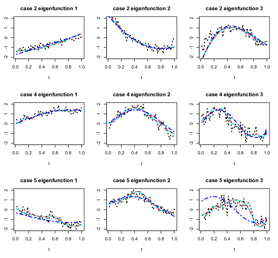
Figure 1: True and estimated eigenfunctions for three cases each with one simulated data set. Each row corresponds to one simulated data set. Each box shows the true eigenfunction (blue dot-dashed lines), the estimated eigenfunction using FACE (red solid lines), the estimated eigenfunction using SSVD (cyan dashed lines), and the estimated eigenfunction without smoothing (black dotted lines). We do not show the estimates from S-Smooth and FACE (incomplete data) because they are almost identical to these from FACE and SSVD.

We compare the performance of the three methods to estimate: (1) the covariance matrix; (2) the eigenfunctions; and (3) the eigenvalues. For simplicity, we only consider the top three eigenvalues/eigenfunctions. For FACE we use 100 knots; for SSVD and S-Smooth we use smoothing splines, implemented through the R function ‘smooth.spline’. Figure 1 displays, for one simulated data set for each case, the true and estimated eigenfunctions using SSVD and FACE, as well as the estimated eigenfunctions without smoothing.

We see from Figure 1 that the smoothed eigenfunctions are very similar and the estimated eigenfunctions without smoothing are quite noisy. The results are expected as all smoothing-based methods are designed to account for the noise in the data and the discrepancy between the estimated and the true eigenfunctions is mainly due to the variation in the random functions. Table 1 provides the mean integrated squared errors (MISE) of the estimated eigenfunctions indicating that FACE and S-Smooth have better performance than SSVD. For case 5, the smoothed eigenfunctions for all methods are far from the true eigenfunctions. This is not surprising because for this case the eigenvalues are close to each other and it is known that the accuracy of eigenfunction estimation also depends on the gap between consecutive eigenvalues; see for example, Bunea and Xiao (2013). In terms of covariance estimation, Table 2 suggests that SSVD is outperformed by the other two methods. However, the simplicity and robustness of SSVD may actually make it quite popular in applications.

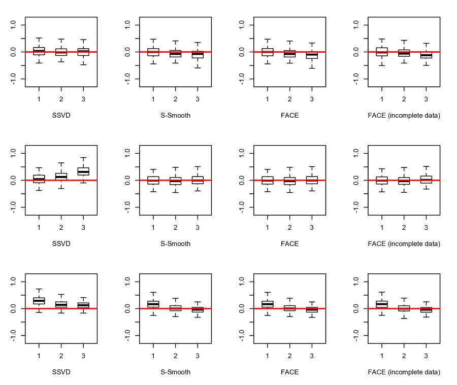
Figure 2: Boxplots of the centered and standardized estimated eigenvalues, ${\widehat{\lambda}}_{k}/\lambda_{k}-1$. The top panel is for case 2, the middle panel is for case 4, and the bottom panel is for case 5. The zero is shown by the solid red line. Case 1 is similar to case 2 and case 3 is similar to case 4, and hence are not shown.

Figure 2 shows boxplots of estimated eigenvalues that are centered and standardized, ${\widehat{\lambda}}_{k}/\lambda_{k}-1$. The SSVD method works well for cases 1 and 2, where the true covariance has only three non-zero eigenvalues, but tends to overestimate the eigenvalues for the other three cases, where the covariance function has an infinite number of non-zero eigenvalues. In contrast, the FACE and S-Smooth estimators underestimate the eigenvalues for the simple cases 1 and 3 but are much closer to the true eigenvalues for the more complex cases. Table 3 provides the average mean squared errors (AMSEs) of $\hat{\lambda}_{k}/\lambda_{k}-1$ for $k=1,2,3$, and indicates that S-Smooth and FACE tend to estimate the eigenvalues more accurately.

6.2 Incomplete data

In Section 4.2 we extended FACE for incomplete data, and here we illustrate the extension with a simulation. We use the same simulation setting in Section 6.1 except that for each subject we allow for portions of observations missing completely at random. For simplicity we fix the length of each portion so that $0.065J$ consecutive observations are missing. We allow one subject to miss either 1, 2, or 3 portions with equal probabilities so that in expectation $13\%$ of the data are missing. Note that the real data we will consider later also has about $13\%$ measurements missing.

In Figure 2, boxplots of the estimated eigenvalues are shown. The MISEs of the estimated covariance function and estimated eigenfunctions and the AMSEs of the estimated eigenvalues appear in Tables 2, 1 and 3, respectively. The simulation results show that the performance of FACE degrades only marginally.

6.3 Computation time

We record the computation time of FACE for various combinations of $J$ and $I$. All other settings remain the same as in the first simulation study and we use the eigenfunctions from case 1. For comparison the computation times of SSVD, S-Smooth and the sandwich smoother (Xiao et al. 2013) are also given. Table 4 summarizes the results and shows that FACE is fast even with high-dimensional data while the computation time of the sandwich smoother increases dramatically with $J$, the dimension of the problem. For example it took FACE only 5 seconds to smooth a 10,000 by 10,000 dimensional matrix for $500$ subjects, while the sandwich smoother did not run on our computer. While SSVD, S-Smooth and FACE are all fast to compute, FACE is computationally faster when $I=500$. We note that S-Smooth has additional problems when data are missing, though a method similar to FACE may be devised. Ultimately, we prefer the self-contained, fast, and flexible FACE approach.

Although we do not run FACE on ultrahigh-dimensional data, we can obtain a rough estimate of the computation time by the formula $O(JIc)$. Table 4 shows that FACE with 500 knots takes 5 seconds on data with $(J,I)=(10000,500)$. For data with $J$ equal to 100,000 and $I$ equal to 2,000, FACE with 500 knots should take 4 minutes to compute, without taking into account the time for loading data into the computer memory. Our code was written and run in R, so a faster implementation of FACE may be possible on other software platforms.

7 Example

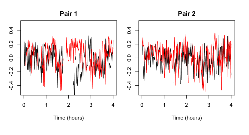
Figure 3: Data for two matched pairs of case and controls in the Sleep Heart Health Study. The red lines are for cases while the black are for controls. For simplicity only the last observation in each minute of the 4-hour interval is shown.

The Sleep Heart Health Study (SHHS) is a large-scale study of sleep and its association with health-related outcomes. Thousands of subjects enrolled in SHHS underwent two in-home polysomnograms (PSGs) at multiple visits. Two-channel electroencephalographs (EEG), part of the PSG, were collected at a frequency of 125Hz, or 125 observations per second for each subject, visit and channel. We model the proportion of $\delta$-power which is a summary measure of the spectrum of the EEG signal. More details on $\delta$-power can be found in Crainiceanu et al. (2009) and Di et al. (2009). The data contain 51 subjects with sleep-disordered breathing (SDB) and 51 matched controls; see Crainiceanu et al. (2012) and Swihart et al. (2012) for details on how the pairs were matched. An important feature of the EEG data is that long consecutive portions of observations, which indicate wake periods, are missing. Figure 3 displays data from 2 matched pairs. In total about $13\%$ of the data is missing.

Similar to Crainiceanu et al. (2012), we consider the following statistical model. The data for proportion of $\delta$-power are pairs of curves $\{Y_{iA}(t),Y_{iC}(t)\}$, where $i$ denotes subject, $t=t_{1},\dots,t_{J}\ (J=2,880)$ denotes the time measured in 5-second intervals in a 4-hour sleep interval from sleep onset, $A$ stands for apneic and $C$ stands for control. The model is

$$\left\{\begin{array}[]{l}Y_{iA}(t)=\mu_{A}(t)+X_{i}(t)+U_{iA}(t)+\epsilon_{iA}(t)\\ Y_{iC}(t)=\mu_{C}(t)+X_{i}(t)+U_{iC}(t)+\epsilon_{iC}(t)\\ \end{array}\right.$$ (6)

where $\mu_{A}(t)$ and $\mu_{C}(t)$ are mean functions of proportions of $\delta$-power, $X_{i}(t)$ is a functional process with mean 0 and continuous covariance operator $K_{X}(\cdot,\cdot)$, $U_{iA}(t)$ and $U_{iC}(t)$ are functional processes with mean 0 and continuous covariance operator $K_{U}(\cdot,\cdot)$, and $\epsilon_{iA}(t),\epsilon_{iC}(t)$ are measurement errors with mean 0 and variance $\sigma^{2}$. The random processes $X_{i},U_{iA},U_{iC},\epsilon_{iA}$ and $\epsilon_{iC}$ are assumed to be mutually independent. Here $X_{i}$ accounts for the between-pair correlation of the data while $U_{iA}$ and $U_{iC}$ model the within-pair correlation. The Multilevel Functional Principal Component Analysis (MFPCA) (Di et al. 2009) can be used to analyze data with model (6). One crucial step of MFPCA is to smooth two estimated covariance operators which in this example are $2880\times 2880$ matrices.

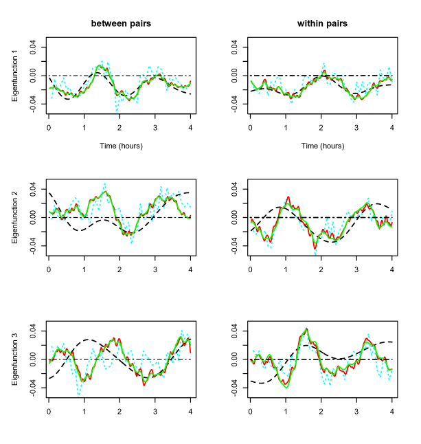
Figure 4: The eigenfunctions associated with the top three eigenvalues of $K_{X}$ and $K_{U}$ for the Sleep Heart Health Study data. The left column is for $K_{X}$ and the right one is for $K_{U}$. The red and green solid lines correspond to the FACE approach using the original and modified GCV, respectively. The black dashed lines are for thin plate splines, and the cyan dotted lines are for SSVD.

Smoothing large covariance operators of dimension $2880\times 2880$ can be computationally expensive. We tried bivariate thin plate regression splines and used the R function ‘bam’ in the mgcv package (Wood 2013) with 35 equally-spaced knots for each axis. The smoothing parameter was automatically selected by ‘bam’ with the option ‘GCV.cp’. Running time for thin plate regression splines was three hours. Because the two covariance operators take the form in Section 4.1 (see the details in Appendix B), we applied FACE, which ran in less than 10 seconds with 100 knots. Note that we also tried thin plate splines with 100 knots in mgcv, which was still running after 10 hours. Figure 4 displays the first three eigenfunctions for $K_{X}$ and $K_{U}$, using both methods. As a comparison, the eigenfunctions using SSVD are also shown. For the SSVD method, to handle incomplete data the SVD step was replaced by a brute-force decomposition of the two $2880\times 2880$ covariance operators. Figure 4 shows that the top eigenfunctions obtained from the two bivariate smoothing methods are quite different, except for the first eigenfunctions on the top row. The estimated eigenfunctions using FACE in general resemble those by SSVD with some subtle differences, while thin plate splines in this example seem to over-smooth the data, probably because we were forced to use a smaller number of knots.

The smoothed eigenfunctions from FACE using PGCV (red solid lines in Figure 4) appear undersmooth. This may be due to the well reported tendency of GCV to undersmooth as well as to the noisy and complex nature of the data. A common way to combat this problem is to use modified GCV (modified PGCV for our case) where ${\textrm{t}r}({\bf S})$ in (2) is multiplied by a constant $\alpha$ that is greater than 1; see Cummins et al. (2001) and Kim and Gu (2004) for such practices for smoothing splines. Similar practice has also been proposed for AIC in Shinohara et al. (2014). We re-ran the FACE method with $\alpha=2$ and the resulting estimates (green solid lines in Figure 4) appear more satisfactory. In this case, the direct smoothing approach of the eigenfunctions (Rice and Silverman 1991; Capra and Müller 1997; Ramsay and Silverman 2005) might provide good results. However, the missing data issue and the computational difficulty associated with large $J$ make the approach difficult to use.

Table 5 provides estimated eigenvalues of $K_{X}$ and $K_{U}$. Compared to FACE (with $\alpha=2$), thin plate splines over-shrink significantly the eigenvalues, especially those of the between pair covariance. The results from FACE in Table 5 show that the proportion of variability explained by $K_{X}$, the between-pair variation, is $14.40/(14.40+22.75)\approx 38.8\%$.

8 Discussion

In this paper we developed a fast covariance estimation (FACE) method that could significantly alleviate the computational difficulty of bivariate smoothing and eigendecomposition of large covariance matrices in FPCA for high-dimensional data. Because bivariate smoothing and eigendecomposition of covariance matrices are integral parts of FPCA, our method could increase the scope and applicability of FPCA for high-dimensional data. For instance, with FACE, one may consider incorporating high-dimensional functional predictors into the penalized functional regression model of Goldsmith et al. (2011).

The proposed FACE method can be regarded as a two-step procedure such as S-Smooth (see, e.g., Besse and Ramsay 1986; Ramsay and Dalzell 1991; Besse et al. 1997; Cardot 2000; Zhang and Chen 2007). Indeed, if we first smooth data at the subject level ${\widehat{\bf Y}}_{i}={\bf S}{\bf Y}_{i},i=1,\dots,I$, then it is easy to show that the empirical covariance estimator of the ${\widehat{\bf Y}}_{i}$ is equal to $\widetilde{{\bf K}}$. There are, however, important computational differences between FACE and the current two-step procedures. First, the fast algorithm in Section 3.2 enables FACE to select efficiently the smoothing parameter. Second, FACE could work with structured functional data and allow for different smoothing for each covariance operator. Third, FACE can be easily extended for incomplete data where long consecutive portions of data are missing while it is unclear how a two-step procedure could be used for such data.

The second approach, SSVD, is very simple and reasonable, though some problems remain open, especially in applications with missing data. Another drawback of SSVD is that the smoothed eigenvectors are not necessarily orthogonal, though the fast Gram-Schmidt algorithm could easily be applied to the smooth vectors. Overall, we found that using a combination of FACE and SSVD provides a reasonable and practical starting point for smoothing covariance operators for high dimensional functional data, structured or unstructured.

In this paper we have only considered the case when the sampling points are the same for all subjects. Assume now for the $i$th sample that we observe ${\bf Y}_{i}=\{Y_{i}(t_{i1}),\dots,Y_{i}(t_{iJ_{i}})\}^{T}$, where $t_{ij}$, $j=1,\ldots,J_{i}$ can be different across subjects. In this case the empirical estimator of the covariance operator does not have a decomposable form. Consider the scenario when subjects are densely sampled and all $J_{i}$’s are large. Using the idea from Di et al. (2009), we can undersmooth each ${\bf Y}_{i}$ using, for example, a kernel smoother with a small bandwidth or a regression spline. FACE can then be applied on the under-smoothed estimates evaluated at an equally spaced grid, $\{{\widehat{\bf Y}}_{1},\dots,{\widehat{\bf Y}}_{I}\}$. Extension of FACE to the sparse design scenario remains a difficult open problem.

Appendix A Appendix: Proofs

Proof of Proposition 1: The design matrix ${\bf B}$ is of full rank (Xiao et al. 2012). Hence ${\bf B}^{T}{\bf B}$ is invertible and ${\bf A}_{S}$ is of rank $c$. ${\hbox{\hbox to0.0pt{$\Sigma$\hss}\kern 0.25pt\hbox to0.0pt{$\Sigma$\hss}\kern 0.25pt$\Sigma$}}_{S}$ is a diagonal matrix with all elements greater than 0 and ${\widetilde{\bf Y}}$ is of rank at most $\min(c,I)$. Hence ${\widetilde{\bf K}}={\bf A}_{S}\left(I^{-1}{\hbox{\hbox to0.0pt{$\Sigma$\hss}\kern 0.25pt\hbox to0.0pt{$\Sigma$\hss}\kern 0.25pt$\Sigma$}}_{S}{\widetilde{\bf Y}}{\widetilde{\bf Y}}^{T}{\hbox{\hbox to0.0pt{$\Sigma$\hss}\kern 0.25pt\hbox to0.0pt{$\Sigma$\hss}\kern 0.25pt$\Sigma$}}_{S}\right){\bf A}_{S}^{T}$ has a rank at most $\min(c,I)$ and the proposition follows.

Proof of Proposition 2: First of all, ${\textrm{t}r}(\mathbf{S})={\textrm{t}r}({\hbox{\hbox to0.0pt{$\Sigma$\hss}\kern 0.25pt\hbox to0.0pt{$\Sigma$\hss}\kern 0.25pt$\Sigma$}}_{S})$ which is easy to calculate. We now compute $\sum_{i=1}^{I}\|{\bf Y}_{i}-{\bf S}{\bf Y}_{i}\|^{2}$. Because $\|{\bf Y}_{i}-{\bf S}{\bf Y}_{i}\|^{2}={\bf Y}_{i}^{T}({\bf S}-{\bf I}_{J})^{2}{\bf Y}_{i}={\textrm{t}r}\{({\bf S}-{\bf I}_{J})^{2}{\bf Y}_{i}{\bf Y}_{i}^{T}\}$,

$$\sum_{i=1}^{I}\|{\bf Y}_{i}-{\bf S}{\bf Y}_{i}\|^{2}={\textrm{t}r}\left\{({\bf S}-{\bf I}_{J})^{2}\sum_{i=1}^{I}{\bf Y}_{i}{\bf Y}_{i}^{T}\right\}={\textrm{t}r}\left\{({\bf S}-{\bf I}_{J})^{2}{\bf Y}{\bf Y}^{T}\right\}.$$

It can be shown that ${\bf S}^{2}={\bf A}_{S}{\hbox{\hbox to0.0pt{$\Sigma$\hss}\kern 0.25pt\hbox to0.0pt{$\Sigma$\hss}\kern 0.25pt$\Sigma$}}_{S}^{2}{\bf A}_{S}^{T}$. Hence ${\textrm{t}r}({\bf S}^{2}{\bf Y}{\bf Y}^{T})={\textrm{t}r}({\bf Y}^{T}{\bf S}^{2}{\bf Y})={\textrm{t}r}({\widetilde{\bf Y}}^{T}{\hbox{\hbox to0.0pt{$\Sigma$\hss}\kern 0.25pt\hbox to0.0pt{$\Sigma$\hss}\kern 0.25pt$\Sigma$}}_{S}^{2}{\widetilde{\bf Y}})={\textrm{t}r}({\hbox{\hbox to0.0pt{$\Sigma$\hss}\kern 0.25pt\hbox to0.0pt{$\Sigma$\hss}\kern 0.25pt$\Sigma$}}_{S}^{2}{\widetilde{\bf Y}}{\widetilde{\bf Y}}^{T})$. Similarly, we derive ${\textrm{t}r}({\bf S}{\bf Y}{\bf Y}^{T})={\textrm{t}r}({\hbox{\hbox to0.0pt{$\Sigma$\hss}\kern 0.25pt\hbox to0.0pt{$\Sigma$\hss}\kern 0.25pt$\Sigma$}}_{S}{\widetilde{\bf Y}}{\widetilde{\bf Y}}^{T})$. We have ${\textrm{t}r}({\bf Y}{\bf Y}^{T})=\|{\bf Y}\|_{F}^{2}$. It follows that

$$\sum_{i=1}^{I}\|{\bf Y}_{i}-{\bf S}{\bf Y}_{i}\|^{2}={\textrm{t}r}\left\{({\hbox{\hbox to0.0pt{$\Sigma$\hss}\kern 0.25pt\hbox to0.0pt{$\Sigma$\hss}\kern 0.25pt$\Sigma$}}_{S}-{\bf I}_{c})^{2}{\widetilde{\bf Y}}{\widetilde{\bf Y}}^{T}\right\}-\|{\widetilde{\bf Y}}\|_{F}^{2}+\|{\bf Y}\|_{F}^{2}.$$

Proposition 3.

The computation time of FACE is $O\left(IJc+Jc^{2}+c^{3}+ck_{0}\right)$, where $k_{0}$ is the number of iterations needed for selecting the smoothing parameter (see Section 3.2), and the total required computer memory is $O\left(JI+I^{2}+Jc+c^{2}+k_{0}\right)$ memory units.

Proof of Proposition 3: We need to compute or store the following quantities: ${\bf X}$, ${\bf B}$, ${\bf B}^{T}{\bf B}$, $({\bf B}^{T}{\bf B})^{-1/2}$, ${\bf P}$, $({\bf B}^{T}{\bf B})^{-1/2}{\bf P}({\bf B}^{T}{\bf B})^{-1/2}$, ${\bf A}_{S}$, ${\widetilde{\bf Y}}$, ${\bf A}$, ${\bf U}$, and ${\bf A}_{S}{\bf A}$. For the computational complexity, ${\bf B}^{T}{\bf B}$, ${\bf A}_{S}={\bf B}({\bf B}^{T}{\bf B})^{-1/2}{\bf U}$, and ${\bf A}_{S}{\bf A}$ require $O(Jc^{2})$ computations; $({\bf B}^{T}{\bf B})^{-1/2}$, ${\bf P}$, $({\bf B}^{T}{\bf B})^{-1/2}{\bf P}({\bf B}^{T}{\bf B})^{-1/2}$, ${\bf A}$, and ${\bf U}$ require $O(c^{3})$ computations; ${\widetilde{\bf Y}}={\bf A}_{S}^{T}{\bf Y}$ requires $O(JIc)$ computations. So in total, $O(JIc+Jc^{2}+c^{3})$ computations are required. For the memory burden, the loading of ${\bf Y}$ requires $O(JI)$ memory units, computer of ${\bf B}$ and ${\bf A}_{S}{\bf A}$ requires $O(Jc)$ memory units, and other objects require $O(c^{2})$ memory units.

Proof of Theorem 1: We have ${\widehat{\hbox{\hbox to0.0pt{$\xi$\hss}\kern 0.25pt\hbox to0.0pt{$\xi$\hss}\kern 0.25pt$\xi$}}}_{i}=J^{-1/2}({\bf A}_{S}{\widehat{\bf A}}_{N})^{T}{\bf Y}_{i}=J^{-1/2}{\widehat{\bf A}}_{N}^{T}({\bf A}_{S}^{T}{\bf Y}_{i})=J^{-1/2}{\widehat{\bf A}}_{N}^{T}{\widetilde{\bf Y}}_{i}$. Proof of Theorem 2: Let ${\widetilde{\bf A}}_{N}$ denote the first $N$ columns of ${\bf A}_{S}{\bf A}$, then ${\widetilde{\bf A}}_{N}={\bf A}_{S}{\widehat{\bf A}}$. The estimated BLUPs for ${\hbox{\hbox to0.0pt{$\xi$\hss}\kern 0.25pt\hbox to0.0pt{$\xi$\hss}\kern 0.25pt$\xi$}}_{i}$ (Ruppert et al. 2003) is

$${\widehat{\hbox{\hbox to0.0pt{$\xi$\hss}\kern 0.25pt\hbox to0.0pt{$\xi$\hss}\kern 0.25pt$\xi$}}}_{i}=J^{-1/2}{\widehat{\hbox{\hbox to0.0pt{$\Sigma$\hss}\kern 0.25pt\hbox to0.0pt{$\Sigma$\hss}\kern 0.25pt$\Sigma$}}}_{N}{\widetilde{\bf A}}_{N}^{T}\left({\widetilde{\bf A}}_{N}{\widehat{\hbox{\hbox to0.0pt{$\Sigma$\hss}\kern 0.25pt\hbox to0.0pt{$\Sigma$\hss}\kern 0.25pt$\Sigma$}}}_{N}{\widetilde{\bf A}}_{N}^{T}+J^{-1}{\widehat{\sigma}}^{2}{\bf I}_{J}\right)^{-1}{\bf Y}_{i}.$$

The inverse matrix in the above equality can be replaced by the following (Seber (2007), page 309, equality b(i)),

$$\left({\widehat{\bf A}}_{N}{\widehat{\hbox{\hbox to0.0pt{$\Sigma$\hss}\kern 0.25pt\hbox to0.0pt{$\Sigma$\hss}\kern 0.25pt$\Sigma$}}}_{N}{\widetilde{\bf A}}_{N}^{T}+J^{-1}{\widehat{\sigma}}^{2}{\bf I}_{J}\right)^{-1}=\frac{J}{{\widehat{\sigma}}^{2}}\left\{{\bf I}_{N}-\frac{J}{{\widehat{\sigma}}^{2}}{\widetilde{\bf A}}_{N}\left({\widehat{\hbox{\hbox to0.0pt{$\Sigma$\hss}\kern 0.25pt\hbox to0.0pt{$\Sigma$\hss}\kern 0.25pt$\Sigma$}}}_{N}^{-1}+\frac{J}{{\widehat{\sigma}}^{2}}{\bf I}_{N}\right)^{-1}{\widetilde{\bf A}}_{N}^{T}\right\}.$$

It follows that

$${\widehat{\hbox{\hbox to0.0pt{$\xi$\hss}\kern 0.25pt\hbox to0.0pt{$\xi$\hss}\kern 0.25pt$\xi$}}} = J^{-1/2}\frac{J}{{\widehat{\sigma}}^{2}}{\widehat{\hbox{\hbox to0.0pt{$\Sigma$\hss}\kern 0.25pt\hbox to0.0pt{$\Sigma$\hss}\kern 0.25pt$\Sigma$}}}\left\{{\bf I}_{N}-\frac{J}{{\widehat{\sigma}}^{2}}\left({\widehat{\hbox{\hbox to0.0pt{$\Sigma$\hss}\kern 0.25pt\hbox to0.0pt{$\Sigma$\hss}\kern 0.25pt$\Sigma$}}}_{N}^{-1}+\frac{J}{{\widehat{\sigma}}^{2}}{\bf I}_{N}\right)^{-1}\right\}{\widehat{\bf A}}_{N}^{T}{\widetilde{\bf Y}}_{i}$$

$$= J^{-1/2}{\widehat{\hbox{\hbox to0.0pt{$\Sigma$\hss}\kern 0.25pt\hbox to0.0pt{$\Sigma$\hss}\kern 0.25pt$\Sigma$}}}_{N}\left({\widehat{\hbox{\hbox to0.0pt{$\Sigma$\hss}\kern 0.25pt\hbox to0.0pt{$\Sigma$\hss}\kern 0.25pt$\Sigma$}}}_{N}+J^{-1}{\widehat{\sigma}}^{2}{\bf I}_{N}\right)^{-1}{\widehat{\bf A}}_{N}^{T}{\widetilde{\bf Y}}_{i}.$$

Appendix B Appendix: Empirical covariance operators for $K_{X}$ and $K_{U}$

Let $I$ denote the number of pairs of cases and controls. For simplicity, we assume estimates of $\mu_{A}(t)$ and $\mu_{C}(t)$ have been subtracted from $Y_{iA}$ and $Y_{iC}$, respectively. Let ${\bf Y}_{iA}=(Y_{iA}(t_{1}),\dots,Y_{iA}(t_{T}))^{T}$ and ${\bf Y}_{iC}=(Y_{iC}(t_{1}),\dots,Y_{iC}(t_{J}))^{T}$. By Zipunnikov et al. (2011), we have estimates of the covariance operators,

$${\widehat{\bf K}}_{X}=\frac{1}{2I}\sum_{i=1}^{I}\left({\bf Y}_{iA}{\bf Y}_{iC}^{T}+{\bf Y}_{iC}{\bf Y}_{iA}^{T}\right),$$

and

$${\widehat{\bf K}}_{U}=\frac{1}{2I}\sum_{i=1}^{I}\left({\bf Y}_{iA}-{\bf Y}_{iC}\right)\left({\bf Y}_{iA}-{\bf Y}_{iC}\right)^{T}.$$

Let ${\bf Y}_{A}=[{\bf Y}_{1A},\dots,{\bf Y}_{nA}]$, ${\bf Y}_{C}=[{\bf Y}_{1C},\dots,{\bf Y}_{nC}]$ and ${\bf Y}=[{\bf Y}_{A},{\bf Y}_{C}]$. Then ${\bf Y}$ is of dimension $J\times 2I$. It can be shown that ${\widehat{\bf K}}_{X}={\bf Y}{\bf H}_{X}{\bf Y}^{T}$ and ${\widehat{\bf K}}_{U}={\bf Y}{\bf H}_{U}{\bf Y}^{T}$, where

$${\bf H}_{X}=\frac{1}{2I}\left(\begin{array}[]{cc}\mathbf{0}_{I}&{\bf I}_{I}\\ {\bf I}_{I}&\mathbf{0}_{I}\end{array}\right),\,\,{\bf H}_{U}=\frac{1}{2I}\left(\begin{array}[]{cc}\mathbf{I}_{I}&-{\bf I}_{I}\\ -{\bf I}_{I}&\mathbf{I}_{I}\end{array}\right).$$

Table 1: $100\times$MISEs of the three methods for estimating the eigenfunctions. The incomplete data has about 13% observations missing.

Eigenfunction No smoothing SSVD S-Smooth FACE FACE incomplete data Case 1 1 9.19 7.27 7.01 6.86 6.97 2 16.95 12.12 11.76 11.65 11.96 3 20.27 6.90 6.74 6.74 6.74 Case 2 1 10.05 6.41 6.39 6.29 6.34 2 17.38 11.13 10.92 10.37 10.46 3 19.71 6.75 6.51 6.08 6.23 Case 3 1 3.14 0.58 0.58 0.58 0.58 2 23.84 4.40 4.37 4.37 4.37 3 55.51 14.07 13.40 13.41 13.14 Case 4 1 5.09 1.81 1.80 1.80 1.87 2 20.14 8.23 8.20 8.20 8.67 3 42.04 19.39 19.39 19.40 20.70 Case 5 1 70.34 64.71 64.71 64.71 65.79 2 96.39 90.57 90.31 90.38 90.84 3 93.09 84.15 83.88 83.99 84.66

Table 2: $100\times$MISEs of the three methods for estimating the covariance function. The incomplete data has about 13% observations missing.

SSVD S-Smooth FACE FACE incomplete data Case 1 9.34 8.96 8.94 8.93 Case 2 8.96 8.64 8.62 8.69 Case 3 1.22 0.76 0.76 0.76 Case 4 0.11 0.07 0.07 0.08 Case 5 2.69 1.98 1.98 2.18

Table 3: $100\times$ average $(\hat{\lambda}_{k}/\lambda_{k}-1)^{2}$ of the three methods for estimating the eigenvalues. The incomplete data has about 13% observations missing.

Eigenvalue SSVD S-Smooth FACE FACE incomplete data Case 1 1 4.37 3.99 3.99 4.31 2 3.43 3.68 3.76 3.96 3 3.97 4.95 5.03 4.99 Case 2 1 4.40 4.05 4.05 4.10 2 3.58 3.78 3.81 3.83 3 3.38 4.02 4.38 4.22 Case 3 1 3.80 3.55 3.55 3.55 2 9.79 3.38 3.38 3.42 3 48.27 4.03 4.03 3.96 Case 4 1 4.22 3.81 3.81 3.84 2 5.65 3.69 3.69 3.64 3 14.77 3.53 3.53 3.43 Case 5 1 12.45 6.45 6.45 7.05 2 4.35 2.09 2.09 2.03 3 3.05 1.64 1.64 1.55

Table 4: Computation time (in seconds) of the SSVD, S-Smooth and FACE methods averaged over 100 data sets on 2.4GHz Mac computers with 8 gigabytes of random access memory. The computation time of the sandwich smoother is also provided except for $J=10,000$ and is averaged over 10 datasets only.

$J$ $I$ SSVD S-Smooth FACE FACE Sandwich Sandwich $100$ knots $500$ knots $100$ knots $500$ knots $3,000$ $50$ 0.25 1.28 0.34 1.76 47.41 210.41 $500$ 3.81 13.88 0.89 2.61 50.91 364.39 $5,000$ $50$ 0.43 2.14 0.50 2.09 251.48 1362.67 $500$ 6.08 34.63 1.26 3.19 302.34 1743.86 $10,000$ $50$ 0.86 4.29 0.82 2.92 - - $500$ 12.78 98.41 2.34 4.68 - -

Table 5: Estimated eigenvalues of $K_{X}$ and $K_{U}$. All eigenvalues are multiplied by $J$ to refer to the variation in the data explained by the eigenfunctions. The row ‘all’ refers to the sum of all positive eigenvalues.

Eigenfunction SSVD FACE Thin Plate Splines $K_{X}$ 1 4.31 3.92 1.91 2 2.64 2.66 0.50 3 1.88 1.35 0.31 all 48.14 14.40 2.81 $K_{U}$ 1 8.84 6.33 6.75 2 5.69 3.18 2.55 3 5.03 2.86 2.04 all 107.95 22.75 12.95

References

- Besse et al. (1997) Besse, P., H. Cardot, and F. Ferraty (1997). Simultaneous nonparametric regressions of unbalanced longitudinal data. Comput. Statist. Data Anal. 24, 255–270.
- Besse and Ramsay (1986) Besse, P. and J. O. Ramsay (1986). Principal components analysis of sampled functions. Psychometrika 51, 285–311.
- Bunea and Xiao (2013) Bunea, F. and L. Xiao (2013). On the sample covariance matrix estimator of reduced effective rank population matrices, with applications to fPCA. To appear in Bernoulli, available at http://arxiv.org/abs/1212.5321.
- Capra and Müller (1997) Capra, W. and H. Müller (1997). An accelerated-time model for response curves. J. Amer. Statist. Assoc. 92, 72–83.
- Cardot (2000) Cardot, H. (2000). Nonparametric estimation of smoothed principal components analysis of sampled noisy functions. J. Nonparametr. Statist. 12, 503–538.
- Crainiceanu et al. (2013) Crainiceanu, C., P. Reiss, J. Goldsmith, L. Huang, L. Huo, F. Scheipl, B. Swihart, S. Greven, J. Harezlak, M. Kundu, Y. Zhao, M. Mclean, and L. Xiao (2013). R package refund: Methodology for regression with functional data (version 0.1-9). URL:http://cran.r-project.org/web/packages/refund/index.html.
- Crainiceanu et al. (2009) Crainiceanu, C., A. Staicu, and C. Di (2009). Generalized Multilevel Functional Regression. J. Amer. Statist. Assoc. 104, 1550–1561.
- Crainiceanu et al. (2012) Crainiceanu, C., A. Staicu, S. Ray, and N. Punjabi (2012). Bootstrap-based inference on the difference in the means of two correlated functional processes. Statist. Med. 31, 3223–3240.
- Craven and Wahba (1979) Craven, P. and G. Wahba (1979). Smoothing noisy data with spline functions. Numer. Math. 31, 377–403.
- Cummins et al. (2001) Cummins, D., T. Filloon, and D. Nychka (2001). Confidence intervals for nonparametric curve estimates: toward more uniform pointwise coverage. J. Amer. Stat. Assoc. 96, 233–246.
- Dauxois et al. (1982) Dauxois, J., A. Pousse, and Y. Romain (1982). Simultaneous nonparametric regressions of unbalanced longitudinal data. J. Multivariate Anal. 12, 136–154.
- Di et al. (2009) Di, C., C. M. Crainiceanu, B. S. Caffo, and N. Punjabi (2009). Multilevel functional principal component analysis. Ann. Appl. Statist. 3, 458–488.
- Eilers and Marx (1996) Eilers, P. and B. Marx (1996). Flexible smoothing with B-splines and penalties (with Discussion). Statist. Sci. 11, 89–121.
- Eilers and Marx (2003) Eilers, P. and B. Marx (2003). Multivariate calibration with temperature interaction using two-dimensional penalized signal regression. Chemometrics and Intelligent Laboratory Systems 66, 159–174.
- Goldsmith et al. (2011) Goldsmith, J., J. Bobb, C. Crainiceanu, B. Caffo, and D. Reich (2011). Longitudinal functional principal component. J. Comput. Graph. Statist. 20, 830–851.
- Greven et al. (2010) Greven, S., C. Crainiceanu, B. Caffo, and D. Reich (2010). Longitudinal functional principal component. Electronic J. Statist. 4, 1022–1054.
- Karhunen (1947) Karhunen, K. (1947). Uber lineare methoden in der wahrscheinlichkeitsrechnung. Annales Academie Scientiarum Fennicae 37, 1–79.
- Kim and Gu (2004) Kim, Y. J. and C. Gu (2004). Smoothing spline Gaussian regression: more scalable computation via efficient approximation. J. R. Statist. Soc. B 66, 337–356.
- Kneip (1994) Kneip, A. (1994). Nonparametric estimation of common regressors for similar curve data. Ann. Statist. 22, 1386–1427.
- Marx and Eilers (2005) Marx, B. and P. Eilers (2005). Multidimensional Penalized Signal Regression. Technometrics 47, 13–22.
- Ramsay and Dalzell (1991) Ramsay, J. and C. J. Dalzell (1991). Some tools for functional data analysis (with Discussion). J. R. Statist. Soc. B 53, 539–572.
- Ramsay and Silverman (2005) Ramsay, J. and B. Silverman (2005). Functional data analysis. New York: Springer.
- Ramsay and Silverman (2002) Ramsay, J. and B. W. Silverman (2002). Applied Functional data analysis: Methods and Case Studies. New York: Springer.
- Rice and Silverman (1991) Rice, J. and B. Silverman (1991). Estimating the mean and covariance structure nonparametrically when the data are curves. J. R. Statist. Soc. B 53, 233–243.
- Ruppert (2002) Ruppert, D. (2002). Selecting the number of knots for penalized splines. J. Comput. Graph. Statist. 1, 735–757.
- Ruppert et al. (2003) Ruppert, D., M. Wand, and R. Carroll (2003). Semiparametric Regression. Cambridge: Cambridge University Press.
- Seber (2007) Seber, G. (2007). A Matrix Handbook for Statisticians. New Jersey: Wiley-Interscience.
- Shinohara et al. (2014) Shinohara, R., C. Crainiceanu, B. Caffo, and D. Reich (2014). Longitudinal analysis of spatio-temporal processes: A case study of Dynamic Contrast-Enhanced Magnetic Resonance Imaging in Multiple Sclerosis. URL:http://biostats.bepress.com/jhubiostat/paper231/.
- Shou et al. (2013) Shou, H., V. Zipunnikov, C. Crainiceanu, and S. Greven (2013). Structured functional principal component analysis. Available at http://arxiv.org/pdf/1304.6783.pdf.
- Staniswalis and Lee (1998) Staniswalis, J. and J. Lee (1998). Nonparametric regression analysis of longitudinal data. J. Amer. Statist. Assoc. 93, 1403–1418.
- Swihart et al. (2012) Swihart, B., B. Caffo, C. Crainiceanu, and N. Punjabi (2012). Mixed effect poisson log-linear models for clinical and epidemiological sleep hypnogram data. Stat. Med. 31, 855–870.
- Wang et al. (2011) Wang, X., J. Shen, and D. Ruppert (2011). Some asymptotic results on generalized penalized spline smoothing. Electronic J. Statist. 4, 1–17.
- Wood (2003) Wood, S. (2003). Thin plate regression splines. J. R. Statist. Soc. B 65, 95–114.
- Wood (2013) Wood, S. (2013). R package mgcv: Mixed GAM computation vehicle with GCV/AIC/REML, smoothese estimation (version 1.7-24). URL:http://cran.r-project.org/web/packages/mgcv/index.html.
- Xiao et al. (2012) Xiao, L., Y. Li, T. Apanasovich, and D. Ruppert (2012). Local asymptotics of P-splines. Available at http://arxiv.org/abs/1201.0708v3.
- Xiao et al. (2013) Xiao, L., Y. Li, and D. Ruppert (2013). Fast bivariate P-splines: the sandwich smoother. J. R. Statist. Soc. B 75, 577–599.
- Yao et al. (2003) Yao, F., H. Müller, A. Clifford, S. Dueker, J. Follett, Y. Lin, B. Buchholz, and J. Vogel (2003). Shrinkage estimation for functional principal component scores with application to the population kinetics of plasma folate. Biometrics 20, 852–873.
- Yao et al. (2005) Yao, F., H. Müller, and J. Wang (2005). Functional data analysis for sparse longitudinal data. J. Amer. Statist. Assoc. 100, 577–590.
- Zhang and Chen (2007) Zhang, J. and J. Chen (2007). Statistical inferences for functional data. Ann. Statist. 35, 1052–1079.
- Zipunnikov et al. (2011) Zipunnikov, V., B. S. Caffo, C. M. Crainiceanu, D. Yousem, C. Davatzikos, and B. Schwartz (2011). Multilevel functional principal component analysis for high-dimensional data. J. Comput. Graph. Statist. 20, 852–873.
- Zipunnikov et al. (2012) Zipunnikov, V., S. Greven, B. S. Caffo, and C. Crainiceanu (2012). Longitudinal high-dimensional data analysis. Available at http://biostats.bepress.com/jhubiostat/paper234/.