Panphasia: a user guide.

Abstract

We make a very large realisation of a Gaussian white noise field, called panphasia, public by releasing software that computes this field. Panphasia is designed specifically for setting up Gaussian initial conditions for cosmological simulations and resimulations of structure formation. We make available both software to compute the field itself and codes to illustrate applications including a modified version of a public serial initial conditions generator. We document the software and present the results of a few basic tests of the field. The properties and method of construction of Panphasia are described in full in a companion paper – Jenkins 2013.

1 Introduction

This document is designed to accompany the software we have released to compute the Panphasia field. We assume that the reader broadly understands what this software is for and has read the introduction of Jenkins (2013) and at least perused the rest of that paper. Our goal for this document is to provide sufficient technical information and guidance to the reader to make using the code relatively straight forward. We are placing this document on the arXiv as we think it will likely need to be updated from time to time – as will the software. We would welcome collaborators interested in modifying or rewriting the code to improve the performance and to provide support for languages other than fortran. We welcome comments on how to improve this document. We would be happy to add additional authors to this document and to expand the acknowledgements section in future versions.

It is not necessary to follow the intricate internal workings of the code to compute Panphasia in order to use it. We have provided the user essentially with a function to compute the properties of Panphasia that can be treated as a black box. It is particularly simple to add Panphasia phases to an initial conditions code used to make ICs for large-scale structure simulations - what we call ‘cosmological initial conditions’. For this application the user code only needs to call two Panphasia subroutines: one subroutine called once to initialise the phases, and a second subroutine called repeatedly to evaluate the field over a three dimensional cubic grid.

We provide a set of subroutines with greater functionality for users interested in making resimulation initial conditions. We describe a method and provide reference calculations and examples in Jenkins (2013) to help with this. ARJ would be happy to provide advice on making resimulation initial conditions using Panphasia.

As well as providing the code to compute Panphasia, we have also included several demonstration codes. These include a version of a public serial code that has been modified so that it can make cosmological initial conditions with Panphasia phases.

In Section 2 we give an overview of Panphasia and how it can be used to publish phase information. In Section 3 we give an overview of the main subroutines we provide for the user for different types of initial condition. In Section 4 we describe the software package itself. In Section 5 we present a few basic tests of Gaussianity of the code. In Section 6 we describe the modifications we make to a public serial initial conditions code so that it can make cosmological initial conditions using Panphasia phases. We list and describe all the subroutines in the appendices.

2 Overview of PANPHASIA

Panphasia is a very large predefined discrete realisation of a Gaussian white noise field with a hierarchical structure based on an octree geometry with 50 octree levels fully populated. It is far too large to be written down in entirety, but any part of Panphasia can be evaluated by calling a function we provide to compute the field. This function is serial and requires only a small amount of memory. A parallel code can simply hold as many private instances of the function as needed.

In Jenkins (2013) we developed a text string, called a phase descriptor that encapsulates the phase information for any given simulation volume. Publishing the phase descriptor in a paper allows others in principle to set up the same simulation volume and even resimulate objects from that volume with no ambiguity as to the phases. The phase descriptor specifies the phases for that volume on all physical scales (down to the CDM free streaming scale if needs be).

To explain the format of the phase descriptor we need first to define a set of coordinates to be used to refer to octree cells. Any cell in an octree at a level $l$ of the tree can be labelled using three Cartesian integer coordinates each in the inclusive range of $0$ to $2^{l}-1$, where (0,0,0) corresponds to a corner cell situated at a particular corner of the root cell of the octree. We will call these coordinates the absolute coordinates of the cell at level $l$. We use these absolute coordinates to define the phase descriptor.

A typical descriptor looks like this:

[Panph1,L11,(200,400,800),S3,CH439266778,MW7]

The descriptor uses five integers to define a cubic region made of whole cells within the root cell of the octree. The first of these integers (11) specifies the shallowest level of the octree needed to define the cube. The next three integers (200,400,800) are the absolute coordinates that label the octree cell at level 11 that lies at the corner of the selected cube closest to the coordinate origin at (0,0,0). The next integer (3), gives the size of the cube in units of octree cells at level 11. Thus the cell furthest from the coordinate origin in the cube has absolute coordinates (202,402,802).

The large integer (439266778) is a check digit that is computed from the properties of Panphasia at the location of the cube (full details are given in Jenkins (2013), appendix B). The check digit provides a way to detect for example a typo in a published phase descriptor. As such a mistake will completely change the phase information for the volume it is important to know that is there. The last string, ‘MW7’, of the descriptor is a human readable name for the phases. In this case it names the phases used for Virgo Consortium’s Millennium simulation run with WMAP7 cosmological parameters. The name can be up to 20 characters long with no spaces.

Strictly speaking the phase descriptor defines a cubic 3-torus within Panphasia. This is because the phases are defined by the Gaussian white noise field within this cube assuming periodic boundary conditions. In general a 3-torus could be a cuboid, but the software we provide assumes a cubic 3-torus. This is by far the most common boundary condition used for cosmological simulations. If there is a demand for support for a more general cuboid then let ARJ know.

Once a 3-torus has been selected by using a phase descriptor there is no need to use absolute coordinates to specify the octree cells within it. Instead our software uses relative Cartesian coordinates to label cells in the 3-torus. The user can choose the position of the origin for these relative coordinates. The relative coordinates are non-negative integers, and obey the periodic boundary conditions of the 3-torus.

Finally, we provide a subroutine to generate new descriptors as it is non-trivial to generate phase descriptors by hand because of the need to compute the check digit.

3 Overview of the software from the point of use

The software provides a set of subroutines that can be called by the user’s code. There are two types of application that we envisage and it is useful to consider these separately:

• Initial conditions for cosmological simulations. These are for uniform mass resolution simulations of periodic cubic volumes (or 3-tori) as typically used for studying large-scale structure.

• resimulation initial conditions. These require multi-mass particle distributions to focus the computational effort on a sub-region of some larger simulation. This larger simulation volume is a cubic 3-torus. The phases used for any resimulation are implicitly defined by the phase descriptor for the 3-torus as a whole.

The Panphasia and pseudorandom number subroutines and functions are described in greater detail in the appendices.

3.1 Cosmological simulations

There are two Panphasia subroutines that need to be called by the user’s program. There is an initialisation routine called, start_panphasia, that takes as input a phase descriptor and a grid size which is an integer. There is an evaluation subroutine called panphasia_cell_properties that returns the values of the Panphasia field for a given cell position.

The value of the grid size implicitly decides which level in the octree is used by panphasia_cell_properties. Taking the phase descriptor given previous section as an example, a value of 3, corresponding to the side-length of the cube at level 11, would select level 11. In general a value of $3\times 2^{n}$ selects level $11+n$. For any other value of the grid size an error message would be produced, as these are the only values that allow a one-to-one correspondence between the octree cells and the grid cells of a three dimensional cubic mesh spanning the periodic simulation volume. Without a one-to-one correspondence it is not possible to accurately reconstruct the phase information.

Because the grid size is quantised in this way it may be wise when defining a new descriptor to choose the number of octree cells on a side with care. Another factor to consider when choosing this value are possible restrictions due to the parallelisation of the initial conditions code. For example a code may distribute a cubic mesh across processors so that each processor has a whole number of planes (e.g. because it uses FFTW 2.1.5). In such a case it may be desirable when running the code for the number of Fourier planes to be exactly divisible by the number of mpi processes running. The number of mpi processes in turn may be determined by the number of cores per node, at least when the code is making optimal use of the hardware. The numbers of cores per node varies between machines and over time, but common values are of the form either $2^{n}$ or $3\times 2^{n}$, where $n$ is a non-negative integer. Choosing a side-length of 3 rather than 1 for the phase descriptor provides more flexibility and we recommend this.

The subroutine panphasia_cell_properties returns the properties of a single octree cell. The routine uses a set of relative coordinates to locate a cell within the 3-torus defined by the phase descriptor and only returns the properties of the cell in this prescribed domain. When the start_panphasia initialisation routine is called the relative coordinate origin (0,0,0) corresponds to the corner cell of the 3-torus that is closest to the absolute origin of Panphasia.

The panphasia_cell_properties subroutine returns nine values for each cell. The first eight are the coefficients of the Legendre block functions for that cell. The Legendre block functions are defined in Section 3.1 of Jenkins (2013). The eight values are ordered as: $p_{000}$, $p_{001}$, $p_{010}$, $p_{011}$, $p_{100}$, $p_{101}$, $p_{110}$, $p_{111}$. The ninth value is independent and not part of the Panphasia field, although as described in Section 5.2 of Jenkins (2013) it may be used in making cosmological initial conditions. These nine values are independent Gaussian pseudorandom numbers drawn from a distribution with zero mean and unit variance.

The cps code, described in Section 6, provides some example code that shows how to combine the nine values returned by panphasia_cell_properties into a single field in $k$-space that can then be used to make cosmological initial conditions in the standard way using Fourier methods.

3.2 Resimulation simulations

We provide a separate set of subroutines with greater functionality for making resimulation initial conditions. Making such ICs typically requires computing the phase information over a series of nested grids or refinements about the region of interest. The extra capabilities include the ability to place the origin of the relative coordinate system at any place within the 3-torus. These relative coordinates obey periodic boundary conditions with respect to the 3-torus and this feature saves the user some bookkeeping. The user can also choose which levels of the octree contribute octree functions to the returned Legendre coefficients of each cell. This gives the user control on how to partition the octree basis functions between the nested grids where they overlap.

The initialisation subroutine in this case is set_phases_and_ref_orign. The first argument is again the phase descriptor. The second is the level of the octree the user requires the Panphasia field to be evaluated. In addition the user can choose the position of the origin used for the relative coordinates within the 3-torus.

For resimulation initial conditions the field is evaluated using a function adv_panphasia_cell_properties which is a generalised version of the subroutine panphasia_cell_properties. The value of the field returned is relative to the origin of the refinement specified by the set_phases_and_refinement subroutine.

The adv_panphasia_cell_properties subroutine allows the user to choose the range of levels of the octree where the octree basis functions are included in the calculation of the returned octree basis function coefficients. The cell properties are returned in an identical structure to that used by panphasia_cell_properties. Because range of octree basis functions can be restricted, the the values returned by this function are no longer necessarily drawn from a Gaussian distribution of zero mean and unit variance.

We also provide a subroutine called layer_choice. This subroutine is used by the ic_2lpt_gen code when making resimulation initial conditions to determine which octree cells are placed on which refinement. See Section 5.3 of Jenkins (2013) and the appendix of this paper for more details.

4 Contents of the software package

The software is packaged as a gzipped tar file called PANPHASIA_code_V1.000.tar.gz. It unpacks to give a top level directory PANPHASIA_public_code which contains a short README file and three subdirectories: src, demo, cps. This README file will be expanded in future versions to include details of revisions to the software.

The directory src contains the source code for computing Panphasia. There are two source files: panphasia_routines.f written by ARJ; and generic_lecuyer.f90 the implementation of mrgk5-93 pseudorandom number (L’Ecuyer et al., 1993) written by SPB. The subroutines in panphasia_routines.f and generic_lecuyer.f90 are listed in Tables 1 and 2. Detailed descriptions of these subroutines are given in the appendices.

The directory demo contains a program file (main.f) and an example makefile. The demonstration code has five different modes. These are described in detail, with examples of the code output provided in the ascii file README_demo. We recommend the user runs these demonstrations and checks the outputs against those illustrated in this README file.

• a subroutine to compute a random descriptor. This provides a convenient way to create descriptors for new simulations.

• a subroutine to calculate the zeroth and first moments of the overdensity field defined by Panphasia over a cuboidal region specified by the user. This provides a test of the code to make sure it is correctly computing the field by comparing the output to that given in the README file.

• a subroutine (random_summation_demo) intended to act as a warning about the code performance when using a close to random access pattern to evaluate Panphasia.

• a subroutine (raster_summation_demo which shows the best and worst raster scan patterns to use for evaluating Panphasia.

• a subroutine (fast_summation_demo) that shows a particularly efficient access pattern suitable suitable for adding to an initial conditions code. We recommend this access pattern is used in parallel applications.

The directory cps contains a version of the serial cosmological initial conditions code Crocce et al. (2006). This code has been modified so that it can read in a Panphasia descriptor. Two example run scripts are provided. See Section 6 for more details.

The underlying structure of Panphasia is completely specified by a large number of predetermined integer values (in fact $>10^{46}$). The values of the field however are floating point numbers that are derived from these integers. The process of generating the floating point values is affected by double precision rounding errors. The exact values of the output floating point numbers will depend on details that effect the order of operations such the particular compiler and the compiler flags used. The differences arising from alternate choices of compilers and optimisation flags are very small in our experience and not a significant concern for the purposes of making cosmological or resimulation initial conditions. We find the speed of the code is sensitive to the compiler flags, and is significantly speeded up with the most aggresive optimisation. However, we advise the user check the effects of different compiler flags themselves. Running the demonstration codes and comparing the output produced with the output shown in README file provides a way to do this.

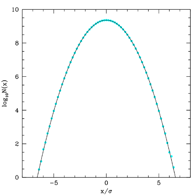
Figure 1: The one-point distribution of the $p_{000}$ Legendre coefficient evaluated over a $3072^{3}$ grid cells for a randomly chosen region in Panphasia. The points show the number of grid cells with values falling within bins of width $0.2\sigma$ centred on zero. The curve shows the expected Gaussian distribution. The agreement is very good. The value of $\sigma$ for the one-point function is unity.

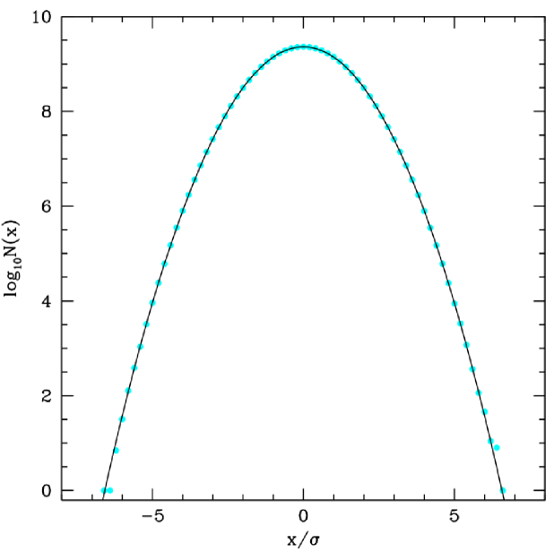
Figure 2: The distribution of values of the two-point cross-correlation function evaluated between the $p_{000}$ and $p_{001}$ Legendre coefficients over a $3072^{3}$ grid cells for the same region as Figure 1. The points show the number of grid cells at non-zero lag with values falling within bins of width $0.2\sigma$ centred on zero. While the plot looks very like Figure 1 the value of $\sigma=1/3072^{3/2}=5.88\times 10^{-6}$ so the fields defined by the $p_{000}$ and $p_{001}$ Legendre coefficients are essentially uncorrelated. The same is true of the other 35 possible cross-correlations and the 9 autocorrelation functions at non-zero lag.

5 Test of the PANPHASIA code

We present some basic tests of the Panphasia code for a region specifed by a phase descriptor. We evaluate the field over a large three dimensional grid. For each grid point the panphasia_cell_properties routine returns nine values.

We expect that the one-point distribution of each of these nine values should accurately follow a Gaussian distribution with zero mean and unit variance. The two-point correlation function evaluated over the grid for each set of values should be very close to zero except at zero lag. The cross-correlation function between any two sets of values should be close to zero at all lags.

While the ensemble averaged auto and cross correlation functions should in general be zero, for a finite sample the most we can expect is that they are very small. For a sample of $N$ grid points we expect the one-point distribution of the cross-correlation functions, and the autocorrelation functions at non-zero lag, to be accurately Gaussian with a mean of zero and a small variance of $1/N$.

For our tests we use a $3072^{3}$ grid, which enables the distribution to be well measured within the range of about $\pm 6$ standard deviations of the expected Gaussian distributions. For the purposes of the test we generated a random phase descriptor:

[Panph1,L40,(592773559564,63351353918,
901943199905),S3,CH1532937555,Test_example]

We have tested other descriptors and get similar results. It is not however practicable to test a significant fraction of the Panphasia field except at low levels of the octree which we do not expect to be used in entirety to make initial conditions anyway.

Figure 1 shows the one-point distribution function for the $p_{000}$ Legendre basis function. Plots for the other eight values look very similar. The level of agreement is excellent even in the tail of the distribution. Taking the 61 bins encompassing the range -6.1 to 6.1 $\sigma$ of the distribution about zero we calculated a $\chi^{2}$ value from the difference of the measured and expected numbers in each bin and obtained a value of 68.2. This is close to the expected value of 61. We conclude the one-point distribution is as expected very close to Gaussian.

We computed the cross and autocorrelation functions of the nine fields using Fourier methods. For all 36 cross-correlation functions, between any two pairs of the nine values returned by panphasia_cell_properties we find the cross-correlation be very small at all lags as expected. The values follow a Gaussian distribution with a variance of $1/3072^{3}$. From the absence of any outliers beyond $7\sigma$ we can set an firm upper limit to the maximum correlation at any lag to be $7/3072^{3/2}=4.1\times 10^{-5}$. For the 9 autocorrelation functions we obtain similar results, after exempting the very strong correlation expected at zero lag. Figure 2 shows the distribution of values for the cross-correlation function between the $p_{000}$ and $p_{001}$ Legendre blocks.

In conclusion we find no evidence for unexpected correlations in these limited test. Passing these tests is necessary, but not sufficient to demonstrate that there are no unwanted correlations in our Gaussian white noise field. We strongly encourage others to test the randomness of Panphasia and report the results to us. We hope to include the results of more tests in future versions of this document.

As we discussed in Jenkins (2013) it is certain that the pseudorandom number generator that we use will fail randomness tests for a sufficiently large sample. Very small deviations from randomness are not obviously a concern for making cosmological initial conditions. If larger deviations are found in other test then these need to be quantified to decide their significance for structure formation simulations. In the worst case it may be necessary to fix the problem - which is a bad from the point of view of publishing phase information as a new phase field would result. The phase descriptor format can accomodate this - although we hope this will not prove necessary.

Deviations from randomness can arise not just from the pseudorandom generator but from mistakes in the software. Indeed the tests in this section are aimed at primarily identifying code errors. We find by deliberately breaking the code that small errors for example in the coefficients defining the octree basis functions are readily detected. The accidental use of the pseudorandom numbers more than once also can be detected. ARJ tested the pseudorandom number routines written by SPB by writing his own generator. This allowed testing that the pseudorandom sequence was correctly being mapped to the octree.

6 An example of adding PANPHASIA to code

As part of the code distribution we provide a modified version of a serial initial conditions generator that accompanied the paper Crocce et al. (2006). The code for this is in the cps directory. We will refer to the code as the cps code.

We have made fairly minimal alterations to the original code. The main change we have made is to separate the part where the phases are set, from the part where the Zeldovich displacements are computed in $k$-space. This makes it easy to put a conditional statement in the code the provides the user with a choice to use original method of setting up the phases, or phases derived from an input Panphasia phase descriptor.

The main addition to the code is a new subroutine called initialise_wnf that calculates the Panphasia phases. This subroutine is placed in a separate file called set_up_wn_field.f and has extensive comments. The initialise_wnf subroutine is called once from the main program.

The cps code makes 2lpt initial conditions. To do this it needs to store six values per grid cell. The initialise_wnf subroutine is able to use these grids as temporary storage. As a result the addition of Panphasia phases to this code does not increase the memory requirements. It is however necessary to call the subroutine that returns the properties of Panphasia twice per grid cell. This is because the routine returns nine numbers per grid cell - only six of which can be stored at one time. The initialise_wnf subroutine combines these nine numbers into a single $k$-space field that reproduces the Panphasia phases in a two stage process: Stage 1 – taking first five values on five separate grids and combining them into a single grid in $k$-space; Stage 2 – assigning the remaining four to four new grids and combining these again in $k$-space together with the single grid from stage 1 into a final single field. This field is then passed back to the main program and used to generate the initial conditions in the same way as was done in the original code.

Based on limited experience we have found that the process of adding a new method for setting phases to an initial conditions code can prove tricky in practice. Even when the new method is almost working the output initial conditions may still bare no obvious obvious resemblance to what is expected! It is advisable to make initial conditions at high redshift so that the output is a close to a linear function of the input phases. Because the process of making the initial conditions is essentially linear it is a good idea to focus on getting the phase and amplitude of single Fourier mode right before attempting to get multiple modes to work. The step from getting a single mode to multiple modes working is not always completely simple.

Our first attempt to add Panphasia phases to the cps code was at first only partially successful. After first focusing on getting the normalisation of the waves correct, we observed that individual modes in the output initial conditions had phases that were either plus or minus $\pi/2$ in phase different from that given by Panphasia. The reason for these shifts is due to the absence of factors of $i$ in the computation of the Zeldovich displacements in the cps main program. As our aim was to change the original cps code as little as possible, we corrected these unwanted phase shifts in the output initial conditions by adding a series of $\pi/2$ phases changes to each mode at the end of the initialise_wnf subroutine. These shifts simply compensate for what is essentially a ‘feature’ of this particular code.

Once this was done then we then found good agreement, at close to single precision round-off, between the cps code Zeldovich initial conditions and Zeldovich initial conditions produced by the ic_2lpt_gen code. To get this level of agreement it was necessary to use slightly different values of the $\sigma_{8}$ parameter in the two codes because the power spectrum normalisation in the cps code is not as accurate as in ic_2lpt_gen. It is also crucial to be sure that exactly the same modes are being set by both codes. Differences in the modes used between initial conditions code usually arise because of different ways of imposing a high $k$ cut-off are used. The modified cps code uses the same sharp spherical cut-off as ic_2lpt_gen for Panphasia phases.

We have included two run scripts for the cps code. These are: run_zeld.sh which produces the initial conditions that we used in our testing against the ic_2lpt_gen code, and dove_example384.sh which generates cosmological initial conditions for the dove volume used in the test simulations in Section 6 of Jenkins (2013). Running these dove initial conditions with the Gadget-2 code (Springel, 2005) to redshift zero we are able to locate the Milky-way mass halo studied in Jenkins (2013) at the expected location. The halo is reproduced with only about 2000 particles at this resolution. We do find a halo close to the correct position and mass. This is very unlikely to be a coincidence. The position of the halo is reproduced to a few tens of kiloparsecs and mass to a few percent of the values given in Jenkins (2013). We provide the Gadget-2 parameter file Gadget2/dove_cps_384.param that we used to run this simulation in our software package.

Appendix A Description of the panphasia_routines code

In this appendix we list all of the subroutines in the file panphasia_routines.f and describe their inputs and outputs and what they do. We list them in the order they occur in the file.

A.1

SUBROUTINE start_panphasia(descriptor,Ngrid)

CHARACTER*100, INTENT(IN)::string

INTEGER, INTENT(IN)::Ngrid

This subroutine needs to be called be a user code making cosmological initial conditions. The descriptor is a character string holding a Panphasia phase descriptor. Ngrid is the size of a cubic grid that spans the 3-torus defined by the descriptor. The value of Ngrid must be a power of two times the integer value prefixed with an ‘S’ in a given descriptor. This restriction is necessary to ensure a one-to-one correspondence between octree cells and the grid that it is being assigned.

A.2

SUBROUNTINE set_phases_and_rel_origin(descriptor,

lev, ix_rel,iy_rel,iz_rel)

CHARACTER*100, INTENT(IN)::descriptor

INTEGER*8, INTENT(IN)::ix_rel,iy_rel,iz_rel

CHARACTER*20, INTENT(IN)::phase_name

A more general initialisation routine. The routines takes a Panphasia phase descriptor as a first argument, but requires the user to explicitly set the level of the octree that will be used to return the properties of the field. The parameters ix_rel,iy_rel,iz_rel define the origin of the relative coordinate system, at level lev of the octree, used to evaluate the field. For resimulations this origin is typically placed at a corner cell of a cubic refinement. The values of ix_rel,iy_rel,iz_rel are constrained to lie within the 3-torus. The relative coordinates obey the periodic boundary conditions of the 3-torus and each component must be non-negative.

Label	Panphasia subroutines	Called by	Calls
A1	start_panphasia	C	A2,11
A2	set_phases_and_rel_origin	R	A3,11,13
A3	initialise_panphasia	A1,2	–
A4	panphasia_cell_properties	C,D	A5
A5	adv_panphasia_cell_properties	R,A4	A6
A6	return_cell_props	A5	A7,8,10
A7	evaluate_panphasia	A6	–
A8	reset_lecuyer_state	A6	A9
A9	advance_current_state	A8	–
A10	return_gaussian_array	A6	–
A11	parse_descriptor	R,A1,2,13	–
A12	compose_descriptor	A14,18	–
A13	validate_descriptor	A2,14,18	A11
A14	generate_random_descriptor	D	–
A15	demo_basis_function_allocator	–	A16,17
A16	layer_choice	R,A15	A17
A17	inref	A16	–
A18	set_local_box	D	A3,12,13

Table 1: Panphasia subroutines and their dependencies. The label ‘C’ represents an intial conditions code for making cosmological initial conditions. Such a code would only need to call subroutines A1 and A4 directly. The label ‘R’ represents an initial conditions code for making resimulation initial conditions (e.g. ic_2lpt_gen). The label ‘D’ represents one or other of the demonstration subroutines that are packaged with the software. The labels refer to the appropriate subsections in appendix A where the routines are described in detail.

A.3

SUBROUTINE initialise_panphasia

Not called directly be the user. This subroutine initialises both mrgk5-93 generator and Panphasia.

A.4

SUBROUTINE panphasia_cell_properties(ix,iy,iz,

cell_prop)

INTEGER, INTENT(IN)::ix,iy,iz

REAL*8, INTENT(OUT)::cell_prop(9)

A basic function to evaluate the Legendre basis function coefficients suitable for making cosmological initial conditions. The cell location is given by relative integer coordinates (ix,iy,iz). These relative coordinates are implicitly determined by an earlier call to start_panphasia. The values of the expansion coefficients are returned in the structure, cell_prop(9). The first 8 values of cell_prop are the Legendre block expansion coefficients of Panphasia for that particular cell. The ninth entry is an independent pseudorandom Gaussian number that is not part of Panphasia. In Jenkins (2013) this ninth value is used to construct an independent Gaussian field to ensure that cosmological initial conditions are isotropic at small scales.

The first eight entries for the cell_data array are the Legendre block coefficients ordered as: $p_{000}$, $p_{001}$, $p_{010}$, $p_{011}$, $p_{100}$, $p_{101}$, $p_{110}$, $p_{111}$. All nine numbers are drawn from a Gaussian distribution with zero mean and unit variance.

A.5

SUBROUTINE adv_panphasia_cell_properties(ix,

iy,iz,layer_min,layer_max,indep_field,

cell_prop)

INTEGER, INTENT(IN)::ix,iy,iz

INTEGER, INTENT(IN)::layer_min,layer_max,

INTEGER, INTENT(IN)::indep_field

REAL*8, INTENT(OUT)::cell_prop(9)

This is a more sophisticated version of the panphasia_cell_properties subroutine described above. It has three extra arguments that can be used to control the range of levels of the octree basis functions used to compute the Legendre block coefficients. This extra functionality is needed for making resimulation initial conditions. As above the cell location is given by relative integer coordinates (ix,iy,iz). These relative coordinates are determined by an earlier call to either start_panphasia or more usually set_phases_and_rel_origin. The values of the expansion coefficients are returned in the structure, cell_prop(9), and depend on exactly which octree basis functions are included. The octree functions selected is controlled by the parameters layer_min and layer_max which determine which levels of the octree are populated with the octree basis functions. For cosmological initial conditions the natural choice for these are 0 and lev so that all the possible octree functions are used.

The subroutine returns the Legendre block expansion coefficients as an array of dimension 9 in the same order as panphasia_cell_properties. The ninth entry is not properly part of Panphasia and the output value also depends on the value of the input integer indep_field. If this integer is 0 then the value returned is also zero. If it 1 then the returned value is an independent Gaussian pseudorandom number drawn from a distribution of mean zero and unit variance. A value of -1 for indep_field results in the independent field being returned and the Legendre basis coefficients all set to zero. This is just testing purposes.

A.6

SUBROUTINE return_cell_props(lev_input,ix_half,

iy_half,iz_half,px,py,pz,layer_min

layer_max,indep_field,cell_data)

INTEGER, INTENT(IN)::lev_input, ix_half,

INTEGER, INTENT(IN)::iy_half, iz_half

INTEGER, INTENT(IN)::px,py,pz, layer_min

INTEGER, INTENT(IN)::layer_max

REAL*8, INTENT(OUT)::cell_data(9,0:7)

Not called by the user. This routine manages the stored octree. The code holds at most eight octree cells at each level of the tree all focused about a particular spatial location within the root cell. If the user requests a value of the field which lies outside of any of the known cells, the relevant parts of the octree are rebuilt to include the new location. Some of the information for the previous location is then lost. A random access pattern of the field therefore requires a lot of computation and is best avoided. If the value of the field has already been computed and is currently being stored then the routine simply returns the values and avoids doing a new computation.

A.7

SUBROUTINE evaluate_panphasia(nlev,leg_coeff,

maxdim,gauss_list,layer_min,layer_max,indep_field,

icell_name, cell_data)

INTEGER, INTENT(IN)::nlev ,maxdim

REAL*8, INTENT(IN)::gauss_list(*)

INTEGER, INTENT(IN)::layer_min,layer_max

INTEGER, INTENT(IN)::indep_field

INTEGER, INTENT(IN)::icell_name

REAL*8, INTENT(INOUT)::leg_coeff(0:7,0:7,

                                                                  -1:maxdim)

REAL*8, INTENT(OUT)::cell_data

Not called by the user. This routine calculates the Legendre basis function coefficients for the eight child cells of a given parent octree cell. These coefficients depend on both the Legendre basis function coefficients of the parent cell, and the octree basis functions belonging to the parent cell. The routine combines the information from these two sources of information to calculate the Legendre basis function coefficients of all eight child cells.

This calculation is done following the definitions of the octree basis functions given at the start of appendix A of Jenkins (2013). The subroutine is well commented.

A.8

SUBROUTINE reset_lecuyer_state(lev,xcursor,

ycursor,zcursor)

INTEGER, INTENT(IN)::lev

INTEGER*8, INTENT(IN)::xcursor,ycursor,zcursor

Not called by the user. The code keeps a three dimensional ‘cursor’ at each level of the octree that holds the cells of interest. This cursor is positioned to ensure that the correct pseudorandom sequence is chosen for each octree basis function.

A.9

SUBROUTINE advance_current_state(lev,

xcursor,ycursor,zcursor)

INTEGER, INTENT(IN)::lev

INTEGER*8, INTENT(IN)::xcursor,ycursor,zcursor

Not called by the user. A low level routine that ensures that the relevant part of the pseudorandom number sequence is used in each cell of the subroutine return_gaussian_array below.

A.10

SUBROUTINE return_gaussian_array(lev,

ngauss,garray)

INTEGER, INTENT(IN)::lev, ngauss

REAL*8, INTENT(OUT)::garray(0:ngauss-1)

Not called by the user. This routine makes an even number, in practice in the code either eight or sixty-four consecutive calls to the mrgk5-93 routine and uses a Box-Muller transformation to produce eight or sixty-four pseudorandom Gaussian variables with zero mean and unit variance. The precise method used is described in appendix B of Jenkins (2013).

A.11

SUBROUTINE parse_descriptor(string,l,ix,iy,iz,

side1,side2,side3,check_int,name)

CHARACTER*100, INTENT(IN)::string

INTEGER, INTENT(OUT)::l

INTEGER*8, INTENT(OUT)::ix,iy,iz

INTEGER, INTENT(OUT)::side1,side2,side3

INTEGER*8, INTENT(OUT)::check_int

CHARACTER*20, INTENT(OUT)::name

This routine takes a phase descriptor as input and parses it into its constituent parts and returns them. If the descriptor is malformed it will complain. This routine only works for descriptor that defines a cubic volume. Therefore the output values of the sides obey: side1 = side2 = side3.

A.12

SUBROUTINE compose_descriptor(l,ix,iy,iz,

side,check_int,name,string)

INTEGER, INTENT(IN)::l

INTEGER*8, INTENT(IN)::ix,iy,iz

INTEGER, INTENT(IN)::side

INTEGER*8, INTENT(IN)::check_int

CHARACTER*20, INTENT(IN)::name

CHARACTER*100, INTENT(OUT)::string

This routines creates a phase descriptor from the inputs. It does not calculate the check digit. To do this use validate_descriptor described below to calculate the check digit, and then call compose_descriptor again.

A.13

SUBROUTINE validate_descriptor(string,

MYID, check_int)

CHARACTER*100, INTENT(IN)::string

INTEGER, INTENT(IN)::MYID

INTEGER*8, INTENT(OUT)::check_int

This routine performs basic checks on a phase descriptor to see if it makes sense. This includes making sure that the check digit is consistent with the other information in the descriptor. If it finds an error the subroutine it just stops. For the special case where the check digit is -999, and the descriptor is otherwise correct the routine returns the value of the check digit.

A.14

SUBROUTINE generate_random_descriptor(string)

CHARACTER*100, INTENT(OUT)::string

This utility can create new descriptors for the user. It tries to choose them randomly from the Panphasia volume. It uses the unix_timestamp, and some input user specific information to help select the region.

The user is asked the side of the simulation in Mpc/h, so that it can choose which level of the octree to select as most appropriate. This feature is intended to ration the available Panphasia volume so that the user is unlikely to choose phases that have been used before.

We would ask users to respect this scaling when generating descriptors, unless there is a very good reason for not doing so. ARJ will also start using this convention for new simulation volumes.

A.15

SUBROUTINE demo_basis_function_allocator

This code was written to illustrate the function of the next two routines which implement the heuristic scheme discussed in Jenkins (2013) for deciding where to place particular octree basis functions when making resimulation initial conditions.

A.16

SUBROUTINE layer_choice(ix0,iy0,iz0,iref,

nref,ix_abs,iy_abs,iz_abs,ix_per,iy_per,

iz_per,ix_rel,iy_rel,iz_rel,ix_dim,

iy_dim,iz_dim,wn_level,,x_fact

layer_min,layer_max,indep_field)

INTEGER, INTENT(IN):: ix0,iy0,iz0,iref,nref

INTEGER*8, INTENT(IN)::ix_abs(nref),iy_abs(nref)

INTEGER*8, INTENT(IN)::iz_abs(nref),ix_per(nref)

INTEGER*8, INTENT(IN)::iy_per(nref),iz_per(nref)

INTEGER*8, INTENT(IN)::ix_rel(nref),iy_rel(nref)

INTEGER*8, INTENT(IN)::iz_rel(nref)

INTEGER, INTENT(IN)::wn_level(nref),x_fact

INTEGER, INTENT(OUT)::layer_min,layer_max

INTEGER, INTENT(OUT)::indep_field

This subroutine was used by the ic_2lpt_gen code in Jenkins (2013) to implement the resimulation method. Its function is to decide given a set of nested refinements which octree basis functions should be assigned to which refinement as a function of position on a given refinement. It returns the values of the layer_min, layer_max and indep_field which can then be used as inputs to the adv_panphasia_cell_properties subroutine. The values ix0,iy0,iz0 are the relative coordinates of a cell in the iref refinement. This refinement is one of nref, all of which have positions and sizes that are passed as the arguments ix_abs(nref) - iz_rel(nref). The input parameter x_fact affects how the octree cells are placed with respect to the refinement boundaries and is introduced in Jenkins (2013) in Section 5.3.

A.17

SUBROUTINE inref(ixc,iyc,izc,isz,ir1,ir2,

nref,wn_level, ix_abs,iy_abs,iz_abs,

ix_per,iy_per,iz_per,ix_rel,iy_rel,iz_rel,

ix_dim,iy_dim,iz_dim,x_fact,interior,iboundary)

INTEGER, INTENT(IN) ::ixc,iyc,izc,isz,ir1,ir2,

INTEGER, INTENT(IN) ::nref,wn_level

INTEGER*8, INTENT(IN)::ix_abs(nref),iy_abs(nref)

INTEGER*8, INTENT(IN)::iz_abs(nref),ix_per(nref)

INTEGER*8, INTENT(IN)::iy_per(nref),iz_per(nref)

INTEGER*8, INTENT(IN)::ix_rel(nref),iy_rel(nref)

INTEGER*8, INTENT(IN)::iz_rel(nref),ix_dim(nref)

INTEGER*8, INTENT(IN)::iy_dim(nref),iz_dim(nref)

INTEGER, INTENT(IN)::x_fact

INTEGER, INTENT(OUT)::interior, iboundary

Not called by the user. This subroutine returns information on whether a cell of interest is inside or outside of a refinement, and if inside whether it is close to or far from the boundary.

A.18

SUBROUNTINE set_local_box(lev,ix_abs,iy_abs,iz_abs,

ix_per,iy_per,iz_per,iz_per,ix_rel,iy_rel,iz_rel,

wn_level_base,check_int,phase_name)

INTEGER, INTENT(IN)::lev,wn_level_base

INTEGER*8, INTENT(IN)::ix_abs,iy_abs,iz_abs

INTEGER*8, INTENT(IN)::ix_per,iy_per,iz_per

INTEGER*8, INTENT(IN)::ix_rel,iy_rel,iz_rel

INTEGER*8, INTENT(IN)::check_int

CHARACTER*20, INTENT(IN)::phase_name

This is a more general initialisation routine - it does not take a phase descriptor as input, but some of the input parameters can be dervied from a descriptor. The subroutine above parse_descriptor can be used to extract this information from a descriptor. We use this subroutine in one of the demonstration codes.

This subroutine allows the user to define both a 3-torus and a cubic subregion within the 3-torus. Calls to the adv_panphasia_cell_properties subroutine use integer cooordinates which are measured relative to this cubic subregion.

The variable lev refers to the level of the octree required by the user. The origin of the 3-torus is given in absolute coordinates by (ix_abs,iy_abs,iz_abs) at this level. The software we provide requires the 3-torus to be a cube. The side lengths input must all be equal so that ix_per = iy_per = iz_per. The side-length is measured in units of octree cells at level lev of the octree. The relative coordinates (ix_rel,iy_rel,iz_rel) define the origin of a cubic subregion within the 3-torus. The input wn_level_base is the octree level given in the descriptor, check_int is the check digit in the descriptor and phase_name is the name from the descriptor. The routine does a consistency check by first reconstituting the descriptor and then calling the validate_descriptor routine described below. If it finds a descrepancy then it simply crashes the code as something is seriously wrong with the inputs and it is not safe to proceed.

Appendix B The Random number interface.

Although we use the mrgk5-93 generator for Panphasia, the routines we use are general and can be used in principle as an interface for alternate generators. We will describe these routines in their full generality and only occasionally make reference to features that are particular to our implementation.

All random number generators have the same basic structure. Any pseudorandom number generator has a finite number of internal states. These are encoded in a State-type ${\cal S}$. Each time the pseudorandom number generator is called an Update transformation ${\tt Update}$ is applied to the state:

$${\tt Update}({\tt RAND\_STATE}\ {{\cal S}_{i}})\Rightarrow{\tt RAND\_STATE}\ {{\cal S}_{i+1}}$$

The next number in the output sequence is then generated by applying an output function ${\tt Output}$ to the new state:

$${\tt Output}({\tt RAND\_STATE}\ {{\cal S}})\Rightarrow{\tt REAL}\ {{\cal R}}$$

Eventually the pseudorandom number generator will return to one of its previous states and the output sequence will start to repeat itself. The length of this cycle is called the period. The common convention is to have the pseudorandom number generator generate uniformly distributed real numbers in the range $0-1$ ${\cal R}$. More complex number distributions can be derived from these.

Label	Pseudorandom generator routines
B1	Rand_seed
B2	Rand_read
B3	Rand_save
B4	Rand_load
B5	Rand_step
B6	Rand_boost
B7	Rand_set_offset
B8	Rand_add_offset
B9	Rand_mul_offset

Table 2: Functions and subroutines provided in the file generic_lecuyer.f90.

In addition to being able to generate random numbers the package has to provide some mechanism to initialise the state of the generator. For example the user could provide a single integer that is used to seed the generator.

$${\tt Seed}({\tt INTEGER}\ {{\cal I}})\Rightarrow{\tt RAND\_STATE}\ {{\cal S}}$$

The function ${\tt Seed}$ maps all valid states of the integer type ${\cal I}$ to distinct states.

We have to define some mechanism that allows checkpointing of the pseudorandom number generator. For example by providing mapping functions between the state-type and integer variables. It is quite possible that the state-type may have a greater number of valid states than the integer type so an array of integers will required.

$${\tt Save}({\tt RAND\_STATE}\ {{\cal S}})\Rightarrow{\tt INTEGER}\ {{\cal I}({\tt Nstate})}$$

$${\tt Load}({\tt INTEGER}\ {{\cal I}({\tt Nstate})})\Rightarrow{\tt RAND\_STATE}\ {{\cal S}}$$

A pseudorandom number generator that implements stepping, such as mrgk5-93, provides some mechanism to efficiently advance the generator by an arbitrary number of steps in the sequence.

$${\tt Step}({\tt INTEGER}\ {x},{\tt RAND\_STATE}\ {{\cal S}_{i}}) \Rightarrow {\tt RAND\_STATE}\ {{\cal S}_{i+x}}$$

The stepping transformation ${\tt Step}$ is parameterised by an integer $x$ and is equivalent to the update transformation applied $x$ times.

	Fortran-90
The State-type	TYPE(RAND_state)
The Offset-type	TYPE(RAND_offset)
Number of integers to hold state	INTEGER, PARAMETER::Nstate
Is stepping available	LOGICAL, PARAMETER::Can_step
LOGICAL, PARAMETER::Can_reverse

As the period of the cycle may be much greater than can be represented by an integer an offset-type ${\cal O}$ is required to be able to specify all possible step lengths. This gives us a second stepping transformation, the offset transformation ${\tt Boost}$ parameterised by an offset-type.

$${\tt Boost}({\tt RAND\_OFFSET}\ {x},{\tt RAND\_STATE}\ {{\cal S}_{i}})\Rightarrow{\tt RAND\_STATE}\ {{\cal S}_{i+x}}$$

Any arbitrary offset can be constructed from the following operations

1. Create offset-type from integer

   $${\tt INTEGER}\ {x}\Rightarrow{\tt RAND\_OFFSET}\ {{\cal O}_{x}}$$

2. Add two offsets

   $${\tt RAND\_OFFSET}\ {{\cal O}_{x}}+{\tt RAND\_OFFSET}\ {{\cal O}_{y}}\Rightarrow{\tt RAND\_OFFSET}\ {{\cal O}_{x+y}}$$

3. Multiply offset by integer

   $${\tt RAND\_OFFSET}\ {{\cal O}_{x}}\times{\tt INTEGER}\ {y}\Rightarrow{\tt RAND\_OFFSET}\ {{\cal O}_{x\times y}}$$

The use of offset types may allow some of the computation involved in the stepping operation to be pre-calculated when constructing the offset. This may give significant savings if the offset is re-used multiple times. In this case the offset could be a matrix or other operator acting on the state. Therefore we cannot assume that it is possible to extract the numerical value of the offset from an offset type.

Not all algorithms can be stepped efficiently though it is always possible to iterate the generator the required number of times.

The RNG interface defines a number of constants and type definitions that are required by the application code. These definitions must be included as follows:

• USE module-name

Only the module-name is derived from the algorithm all other identifiers are standardised. This requires the minimum changes to the source code to change the algorithm used but still allows a single program to use different generators.

Fortran-90 allows a USE statement to specify a rename-list so one conforming module can be used to construct another (for example by applying a shuffle).

The definitions provided by the package are shown in Table B.

The Can_step parameter is only .TRUE. if the implementation can step the generator more efficiently than just iterating the generator. If it is .FALSE. the stepping functions are not available and the application must either abort or iterate the generator itself.

The Can_reverse parameter is only .TRUE. if negative integers can be specified as input to Rand_step and Rand_set_offset. If it is .FALSE. negative inputs produce undefined behavior. Negative offsets are needed to accurately step “shuffled generators” as the underlying generator must be run backwards to initialise the shuffle-table after each stepping operation.

The routines defined in the package are as follows:

B.1 Seeding the generator

SUBROUTINE Rand_seed(state,n)

TYPE(Rand_state), INTENT(OUT)::state

INTEGER, INTENT(IN)::n

This routine overloads the assignment operator. Where the number of possible states is larger than the number of possible default INTEGER values this routine attempts to produce uncorrelated states even if this results in expensive computation. The integer n should be a positive integer.

B.2 Generating Random numbers.

The following Generic interface is used. This overloads different supported REAL kinds and also scalar/rank-1 vector.

SUBROUTINE Rand_real(target,state)

REAL, INTENT(OUT)::target

TYPE(RAND_state), INTENT(INOUT)::state

Result is uniformly distributed between zero and one, but in the case of our implementation of mrgk5-93 neither zero or one is generated. The set of supported real KINDs must include default REAL but is otherwise un-specified.

B.3 Saving the state

SUBROUTINE Rand_save(save_vec,x)

INTEGER, INTENT(OUT)::save_vec(Nstate)

TYPE(RAND_state), INTENT(IN)::x

This routine overloads the assignment operator.

B.4 Loading the state.

SUBROUTINE Rand_load(state,input)

TYPE(RAND_state), INTENT(OUT)::state

INTEGER, INTENT(IN)::input(Nstate)

This routine overloads the assignment operator.

B.5 Stepping the generator

FUNCTION Rand_step(x,n)

TYPE(Rand_state) Rand_step

TYPE(RAND_state), INTENT(IN)::x

INTEGER, INTENT(IN)::n

B.6 Jumping through the sequence

FUNCTION Rand_boost(x,offset)

TYPE(Rand_state) Rand_boost

TYPE(Rand_state), INTENT(IN)::x

TYPE(Rand_offset), INTENT(IN)::offset

These routines overload the addition operator. If stepping is not available these routines abort the program with an error. The integer n must not be negative unless Can_reverse is true.

B.7 Setting an offset

SUBROUTINE Rand_set_offset(offset,n)

TYPE(Rand_offset), INTENT(OUT)::offset

INTEGER, INTENT(IN)::n

This routine overloads the assignment operator. The integer n must not be negative unless Can_reverse is true.

B.8 Adding two offsets

TYPE(Rand_offset) FUNCTION Rand_add_offset(a,b)

TYPE(Rand_offset), INTENT(IN)::a,b

This routine overloads the addition operator.

B.9 Multiplying two offsets

TYPE(Rand_offset) FUNCTION Rand_mul_offset(a,n)

TYPE(Rand_offset), INTENT(IN)::a

INTEGER, INTENT(IN)::n

This routine overloads the multiplication operator. The integer n must not be negative. If stepping is not available these routines abort the program with an error.

References

- Crocce et al. (2006) Crocce M., Pueblas S., Scoccimarro R., 2006, MNRAS, 373, 369
- Jenkins (2013) Jenkins A., 2013, ArXiv e-prints
- L’Ecuyer et al. (1993) L’Ecuyer P., Blouin F., Couture R., 1993, ACM Transactions on Modeling and Computer Simulation, 3, 87
- Springel (2005) Springel V., 2005, MNRAS, 364, 1105