Algorithm independent bounds on community detection problems and associated transitions in stochastic block model graphs

Abstract

We derive rigorous bounds for well-defined community structure in complex networks for a stochastic block model (SBM) benchmark. In particular, we analyze the effect of inter-community “noise” (inter-community edges) on any “community detection” algorithm’s ability to correctly group nodes assigned to a planted partition, a problem which has been proven to be NP complete in a standard rendition. Our result does not rely on the use of any one particular algorithm nor on the analysis of the limitations of inference. Rather, we turn the problem on its head and work backwards to examine when, in the first place, well defined structure may exist in SBMs. The method that we introduce here could potentially be applied to other computational problems. The objective of community detection algorithms is to partition a given network into optimally disjoint subgraphs (or communities). Similar to $k-$SAT and other combinatorial optimization problems, “community detection” exhibits different phases. Networks that lie in the “unsolvable phase” lack well-defined structure and thus have no partition that is meaningful. Solvable systems splinter into two disparate phases: those in the “hard” phase and those in the “easy” phase. As befits its name, within the easy phase, a partition is easy to achieve by known algorithms. When a network lies in the hard phase, it still has an underlying structure yet finding a meaningful partition which can be checked in polynomial time requires an exhaustive computational effort that rapidly increases with the size of the graph. When taken together, (i) the rigorous results that we report here on when graphs have an underlying structure and (ii) recent results concerning the limits of rather general algorithms, suggest bounds on the hard phase.

I Introduction

Increasingly, data are being generated in the form of networks, where interactions among objects are the focus of study. Social networks are perhaps the most prototypical example which consist of people (nodes) and their associations (edges). Finding structure in complex networks is a problem of broad interest with applications in social, biological, communications systems and many other branches. Generally speaking, “community detection” Fortunato (2010); Newman and Girvan (2004) attempts to identify relevant structure in a complex network by searching for clusters of nodes (which are termed communities) that have a higher density of internal edges (i.e., intra-community links) than they have with other communities (inter-community links)Darst et al. (2013).

A wide variety of methods for community detection have been developed over the past decade Fortunato (2010); Newman and Girvan (2004). More recently, an intense effort has been expended on understanding the theoretical foundations of these methods and of community structure in general. This was underscored by Fortunato and Barthélemy when they demonstrated that maximizing “modularity” Newman and Girvan (2004), a common measure of network partitioning, suffered from a fundamental limitation. Modularity is a global network parameter which measures the quality of any particular network partition. Higher modularity is taken to mean that more meaningful communities are found Newman and Girvan (2004); Newman (2006). A fundamental shortcoming of this method is that the local community partitions determined by maximizing modularity depend on the global size of the network Fortunato and Barthelemy (2007); Lancichinetti and Fortunato (2011).

A prevalent method of judging the performance of community detection algorithms involves “planting” initially well-defined community partitions into a random network in progressively more challenging contexts (more extraneous and/or fewer inter-community edges). A vivid example of such a planted state is provided by the cartoon of Fig. 1 depicting $q=2$ communities, each with $n=8$ nodes, and the internal/external edges associated with a specific node; in this cartoon for each node there are far more internal intra-community edges than links between nodes in different communities. Such benchmarks are generally defined by a set of parameters specifying the edge densities within the planted communities and an amount of “noise” representing additional spurious edges between nodes in different communities. The goal of community detection algorithms, as applied to the particular case of benchmark graphs, is to rediscover the embedded communities in given network with no prior information about the planted partition. Community detection methods are then tested against increasingly challenging benchmarks until detection of viable communities becomes impossible. Common benchmarks of planted partitions include stochastic block models, a benchmark by Lancichinetti, Fortunato, and Raddicchi (LFR) which focuses on power law distributions of nodes and degrees Lancichinetti et al. (2008), and a variety of “real-life networks”. Recent theoretical work studied the limits of various community detection methods with increasing levels of noise.

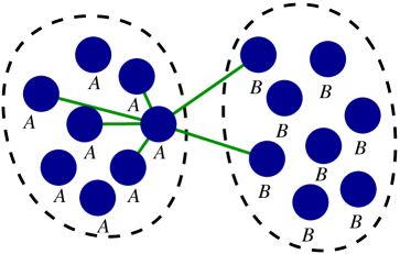
Figure 1: Planted communities. Each node is labeled with its planted community. Example edges of one node of community $A$ is drawn, and we see it has more edges to community $A$ than $B$. Community detection algorithms are thus expected to be able to find that this node belongs to the $A$ community.

In Hu et al. (2011), it was demonstrated that community detection as ascertained by Potts models in rather general random power-law type graphs may exhibit sharp spin-glass type transitions as a function of increasing noise in the limit of large system size. These transitions were evinced via thermodynamic functions, dynamical quantities, and information theoretic overlaps. Various groups have obtained highly noteworthy explicit equations for the transition lines for the community detection problem as applied a particular class of graph, the uniform (or vanishing power law) “stochastic block model” (SBM) on which we further focus on in this paper. As we will elaborate on, SBMs are random graphs defined by a constant number $n$ of nodes per community and fixed intra- and inter-community edge densities. SBMs exhibit a transition whose presence was made very evident in numerical studies of a Potts type approach to community detection as the system size was progressively increased, e.g., Ronhovde and Nussinov (2009). We note the analysis of Decelle, et. al. (DKMZ) Decelle et al. (2011) on the inference of possible assignments of nodes to their proper communities in sparse (i.e., graphs with a small number of links per node) SBM networks which has led to an explicit equation for the detectability threshold. Later stringent results by Mossel, Neeman, and Sly Mossel et al. (2012) on the general limits of Bayesian inference for $q=2$ component sparse graphs concurred (as a bound) with the formula derived by DKMZ via their cavity-type approximations. In an illuminating work, Nadakuditi and Newman (NN) Nadakuditi and Newman (2012) reported on an inherent accuracy limit for modularity-based community detection methods as appplied to SBMs. NN found an expression identical to the earlier result of DKMZ for the threshold of noise beyond which spectral methods cannot resolve the communities. In the analysis of NN, average degree diverges with the network size. After comparing to the earlier result of DKMZ, Nadakuditi and Newman asserted that no method can perform better than modularity on SBM graphs. NN further provided an important additional formula for the fraction of properly detected nodes as a function of noise. It is this formula of NN that largely inspired the current investigation. In what will follow in this article, we will derive lower bounds for such a fraction. Earlier pioneering works are also extremely noteworthy. Amongst others, earlier analysis McSherry (2001) was performed for non-dilute graphs. Based on the cavity approximation, Reichardt and Leone insightfully initially suggested a similar threshold beyond which detection of communities is no longer possible Reichardt and Leone (2008).

In the present work, we will derive universal rigorous bounds on the feasibility of well-defined community structure independent of any specific community detection methods. Our results are related to fundamental, generic properties of community structure and pertain to general networks. We rigorously examine when a benchmark network may have any meaningful structure in the first place. We do this by looking microscopically at each node to determine the ability of any algorithm to properly classify that node: an assertion that each node be more strongly connected (by more edges) to its intended community than to any other community. Due to stochastic fluctuations in edge placement, there typically is a nontrivial (and as we illustrate in this work, computable) number of nodes where this is not the case. We will derive rigorous upper bounds for the fraction of nodes which may be detectable at all. While these calculations lead to an upper bound, they are not necessarily equivalent to a calculation of optimal performance of community detection algorithms. In fact, we find further evidence for a region where graph structure exists but certain methods may not be able to detect it.

We now elaborate in more detail on the stochastic block benchmark and further general reasoning behind benchmark graphs. Although the ideas advanced in our work hold for any system, we will, for concreteness, focus on the stochastic block model (SBM). The SBM is defined as follows. Each node belongs to one community (or “block”) Holland et al. (1983); Heimlicher et al. (2012). The probability of having an edge between two nodes depends solely on their community membership. Specifically, the probability ($p_{\mathrm{out}}$) of having an edge between any pair of nodes belonging to the same community (intra-community edges) is fixed to a certain value $p_{\mathrm{in}}$ and the probability of having an edge between any two nodes that belong to two different blocks (inter-community edges) is given by another uniform value $p_{\mathrm{out}}$.

When a benchmark graph is used, it is assumed that there is a planted community structure which one may (and should if the community detection algorithm is good) consistently detect. Such a planted structure can be thought of being generated by the following gedanken experiment. Imagine that we “plant” a community partition solution by dividing a group of $N$ nodes into $q$ equivalent, completely decoupled, communities of size $n\equiv N/q$ each. Within each community the probability that a given node will be connected by an edge to any other node in the same community is $p_{\mathrm{in}}>0$. An absence of any inter-community links in the initial decoupled state implies that the probability of having a link between any two nodes that belong to different communities is $p_{\mathrm{out}}=0$. In the absence of any such inter-community links, finding the planted communities is a relatively easy task. Next, imagine that more and more edges are added between different communities (i.e., that the probability for outside links (or “noise” ) $p_{\mathrm{out}}$ is progressively increased) while the number of intra-community edges is left unchanged. It is intuitively clear that for “small” $p_{\mathrm{out}}$, finding the planted community will be easy while for sufficiently large $p_{\mathrm{out}}$, the structure of the planted partition will be no longer be well-defined. Previous work shows that the network structure becomes hard to detect at the point $p_{\mathrm{in}}-p_{\mathrm{out}}=\sqrt{\frac{1}{n}\left(p_{\mathrm{in}}+(q-1)p_{\mathrm{out}}\right)}$, which is distinctly different from the point of loss of structure at $p_{\mathrm{in}}=p_{\mathrm{out}}$Decelle et al. (2011); Nadakuditi and Newman (2012). This implies that there are points where there is some nominal structure present in the graph ($p_{\mathrm{out}}<p_{\mathrm{in}}$) yet that structure is undetectable by any method. Instead of focusing on detectability directly, we study the amount of structure which is actually present in the graph.

When the planted communities are, as is the case for sufficiently small $p_{\mathrm{out}}$, reflected in the edge structure, we will term these graphs “well-defined.” An “ill-defined” graph is, for a sufficiently large $p_{\mathrm{out}}$, one in which the assigned edge structure does not reflect the planted communities. An extreme example of an ill-defined graph is afforded by a network in which nodes are assigned (planted) into communities, but then all edges are randomly defined with no preference for intracommunity or inter-community links. No community detection method would be able to detect the purported “communities” in this case as the input (edge structure) is assigned independent of the intended communities. In the above description, well-defined structure is described as a graph property, but it can also be applied to individual nodes. We reiterate that our focus is not simply that of establishing a community detection limit. Rather, we focus on a fundamental limit concerning the creation of such benchmark graphs. Several authors have hinted at this effect in the past, however, it has never been rigorously analyzed and considered as a fundamental limitation of community detection Lancichinetti et al. (2008); Lancichinetti and Fortunato (2009). While we do not directly explain the origin of the detectability threshold in this work, we provide tools to analyze the divergence of structure and detectability.

II Outline

The remainder of this work is organized as follows: We start our discussion with the definition of the SBM problem and our criterion for a well defined community partition. In section III, we set up our formalism and express the problem of a planted state in terms of a binomial distribution. In section IV, we write the corresponding exact expressions for the probability that a planted partition satisfies our criterion for a well defined community partition. We then introduce, in section V, a simple approximation for computing these probabilities. In section VI, we write general exact expressions for the fraction of nodes in the planted partition that satisfy our criterion for community detection. We then turn to illustrate via a trivial application of Jensen’s inequality that the approximation of section VII provides rigorous lower bounds on the probability that our criteria for a well defined partition are satisfied. Armed with all of these formal results for the SBM problem, we then briefly turn to consider their implications. We first consider, in section VIII, threshold values of the noise $p_{\mathrm{out}}$ beyond which well defined community partitions are no longer possible. This will allow for a relation between our results and the phase boundaries of the detectable region of the phase diagram. In section IX, we discuss the abstract meaning of our “well-defined fraction” and make a comparison, between our analysis and that of systems in which ill-defined nodes are shifted to their correct communities. We then discuss, in section X, the breadth of graph types and community detection methods to which our work is applicable. In section XI, we examine the behavior of our well defined transitions as our systems increase in size; we will see that our transitions between well- and ill-defined benchmarks become sharp. In section XII, we compare our limits of well-definedness to other established limits of community detection to see that they agree in a certain limit, with the a region of well-defined but undetectable communities shrinking as our system grows larger. we point out, in section XIII, how high performance algorithms lead to results that coincide, in certain limits, with our computed “well-defined” fraction. In section XIV we discuss possible extensions of our approach to other problems and further note possible bounds on the region where a computationally solvable “hard phase” appears; in this phase, purported solutions of the community detection problem may be easily checkable in polynomial time (as in any NP problemFortnow (2009)) yet finding these solutions (even though they exist) might not be efficiently achieved by general algorithms. We conclude, in section XV, by summarizing our main results with an eye towards their practical significance.

III Binomial distributions of edge densities

As we stated in the Introduction, when formally defined, SBMs constitute benchmark graphs in which planted communities are specified for each node, and edges are assigned between every pair of nodes with a probability $p_{AB}$ which depends only on the communities $A$ and $B$ of the two nodes, respectively. In order for communities to be defined, one would expect that the density of links between communities inside a community $A$ will exceed that between communities $A$ and $B$Darst et al. (2013),

$$p_{\mathrm{in}}=p_{AA}>p_{A,B\neq A}=p_{\mathrm{out}}.$$ (1)

However, we reiterate that in this work, we will show that due to the fluctuations in number of edges connecting a given node to other communities (i.e., not its own), it is possible, in fact likely, to have nodes which are not well-defined in their community even with $p_{AA}$ above the threshold of Eq. (1). Unlike some other particular approaches, Nadakuditi and Newman (2012); Decelle et al. (2011); Mossel et al. (2012); McSherry (2001); Reichardt and Leone (2008); Hu et al. (2011) this is not a limit of a particular community detection method, or limitation on possible inference of structure. Amongst earlier works on SBMs that invoke inference methods, we explicitly re-iterate and note anew the cavity-type approximations of Decelle et al. (2011) and a later non-trivial rigorous result Mossel et al. (2012) partially reaffirming the cavity approximations for when structure in sparse SBMs may be not be inferable for the particular case of $q=2$ communities. Instead of asking whether inference or other methods may succeed, our results relate to the fundamental structure of the graph itself, as suggested in Lancichinetti et al. (2008); Lancichinetti and Fortunato (2009). As such, our results lead to universal intrinsic bounds for any community detection method or inference considerations.

We now turn to the SBM network with $q$ communities of size $n_{A}$ nodes per community $A$ and a total number of nodes $N=\sum n_{A}$, with particular values of $p_{\mathrm{in}}$ and $p_{\mathrm{out}}$. In a random realization of an SBM graph with these parameters, the internal degree $k_{\mathrm{in}}$ of a node to its community $A$ (the “internal degree”) follows the binomial distribution ($\mathcal{B}$) with $n_{A}-1$ attempts to make an edge, each with a probability $p_{\mathrm{in}}$,

$$P[k_{\mathrm{in}}=k]=\mathcal{B}(k;n_{A}-1,p_{\mathrm{in}}).$$ (2)

Associated with any particular single external community $B$, there is a binomial probability distribution of the external degree

$$P[k_{\mathrm{out},B}=k]=\mathcal{B}(k;n,p_{\mathrm{out}}).$$ (3)

The form of the binomial distribution is given at the end of this section. Note that $k_{\mathrm{out},B}$ is the external degree to a specific community $B$, as opposed to the external degree summed over all $(q-1)$ external communities. Also, note that there are $n-1$ possible internal edges since we consider nodes to not link to themselves, but $n$ possible external edges to each external community.

If all communities are of the same size $n$ (i.e., if all communities are comprised of $n$ nodes), we will say that a node $a$ “is well-defined” in its planted community $A$ for this node if there are more internal than external connections to any one external community. That is,

$$k_{\mathrm{out},B}<k_{\mathrm{in}},$$ (4)

for all communities $B\neq A$. One key concept here which bears restatement is that any node can have more external (summed over the other $q-1$ communities) than internal edges and yet still be properly defined in its ground-state community if the many external links are spread out over enough different external communities. We note that this is more relaxed than the Radicchi definition of “weak” community in Radicchi et al. (2004). As numerical results illustrate, we can detect communities well past the weak definition Ronhovde and Nussinov (2010). Zhang and Zhao also point out another intuitive case Zhang and Zhao (2012); Zhang et al. (2009) where the strong and weak definitions of community structure proposed by Radicchi are both violated.

In order to generalize our considerations to unequal sized communities, we employ the edge density $\rho=k/n$ instead of the raw number of linksDarst et al. (2013). For a node to be well-defined in a community, the edge density to that community must be greater than the edge density to any other community. This assumption is discussed later. Then, instead of Eq. (4) our criteria for a well defined community partition are captured in terms of edge densities. That is, for each node in a community $A\neq B$,

$$\rho_{\mathrm{out},B}<\rho_{\mathrm{in}}.$$ (5)

The densities in Eq. (5) are defined as $\rho_{\mathrm{out},B}\equiv\frac{k_{\mathrm{out},B}}{n_{B}}$ and $\rho_{\mathrm{in}}\equiv\frac{k_{\mathrm{in}}}{n_{A}-1}$. Clearly, as the number of conditions of the form of Eq. (5) that need to be checked scale linearly in the system size (i.e., linearly in the number of individual nodes $N$ and linearly in the number of external communities $(q-1)$). Checking a purported partition is a polynomial in time problem (rendering the problem as formulated by Eq. (5) to be of the NP type). However, as in many NP problems, finding correct partition(s) in general networks that satisfy these constraints need not be an easy polynomial problem. (In fact, maximizing the best well known measure for community detection, that of modularity, was shown to be NP complete Brandes et al. (2008, 2007).) As we discussed above, the degrees $k_{\mathrm{in}}$ and $\{k_{\mathrm{out},B}\}_{B\neq A}$ for each individual node follow a binomial distribution. Therefore, the distributions of internal and external edge densities are described as

$$P\left[\rho_{\mathrm{in}}=\frac{k}{n_{A}-1}\right] = \mathcal{B}(k;n_{A}-1,p_{\mathrm{in}}),$$ (6)

$$P\left[\rho_{\mathrm{out}}=\frac{k}{n_{B}}\right] = \mathcal{B}(k;n_{B},p_{\mathrm{out}}),$$ (7)

for $k=0,\ldots,n_{A}-1$ or $k=0,\ldots,n_{B}$ respectively. In the above, we employed the following shorthand for (a normalized) binomial distribution,

$${\mathcal{B}(m;n,p)}={{n}\choose{m}}p^{m}(1-p)^{n-m}.$$ (8)

Away from the dilute limit, we may use a normalized Gaussian to approximate the binomial distribution $\mathcal{B}(m;n,p)\approx\mathcal{N}\left(m;\left<x\right>,\sigma^{2}\right)$ where the binomial mean is $\langle x\rangle=np$ and the variance is $\sigma^{2}=np(1-p)$. The normalized Gaussian is, explicitly, given by

$$\mathcal{N}(x;\left<x\right>,\sigma^{2})=\frac{1}{\sqrt{2\pi\sigma^{2}}}\exp[-[x-\left<x\right>]^{2}/(2\sigma^{2})],$$ (9)

where, in the argument, $\left<x\right>$ specifies the mean of the Gaussian and $\sigma^{2}$ its variance. Employing the normal distribution, Eqs. (6, 7) read

$$P\left[\rho_{\mathrm{in}}=\frac{k}{n_{A}-1}\right] = \mathcal{N}\left(k;(n_{A}-1)p_{\mathrm{in}},(n_{A}-1)p_{\mathrm{in}}(1-p_{\mathrm{in}})\right),$$ (10)

$$P\left[\rho_{\mathrm{out}}=\frac{k}{n_{B}}\right] = \mathcal{N}\left(k;n_{B}p_{\mathrm{out}},n_{B}p_{\mathrm{out}}(1-p_{\mathrm{out}})\right).$$ (11)

We can invoke the identity $\mathcal{N}(mn;np,np(1-p))=\mathcal{N}(m;p,{p(1-p)\over n})$ to simplify the evaluation of these probabilities. In sparse graphs for which $\lim_{n\to\infty}np=\lambda$ with $\lambda$ denoting a constant of order unity, we can approximate the binomial distribution by a Poisson distribution instead of a normal Gaussian distribution. We use the equivalence $\lim_{n\to\infty}\mathcal{B}(m;n,p)\approx\mathrm{Pois}(m;np)=\frac{\lambda^{m}}{m!}\exp[-\lambda]$. That is,

$$P[\rho_{\mathrm{in}}=x] = \mathrm{Pois}(x;(n-1)p_{\mathrm{in}}),$$ (12)

$$P[\rho_{\mathrm{out}}=x] = \mathrm{Pois}(x;np_{\mathrm{out}}).$$ (13)

For very dense graphs ($p\approx 1$), we could conceivably use the Poisson distribution to model missing, rather than existing, edges.

IV Probabilities for well defined communities

In view of Eqs. (4, 5), our goal is to determine the probability that there are not more external links than internal, i.e., to compute

$$P\left[\max_{B}({\rho_{\mathrm{out},B}})<\rho_{\mathrm{in}}\right].$$ (14)

To do this, we observe that the probability for just one external community $B$ to have less links to a given node $a$ in $A$ than all of the links between that given node $a$ and other nodes in the same community $A$ is, from Eqs. (10, 11), given by

$$P\left[\rho_{\mathrm{out},B}<\rho_{\mathrm{in}}\right]=\int dx~{}P\left[0<\mathcal{N}\left(x;p_{\mathrm{in}},{p_{\mathrm{in}}(1-p_{\mathrm{in}})\over n_{A}-1}\right)-\mathcal{N}\left(x;p_{\mathrm{out}},{p_{\mathrm{out}}(1-p_{\mathrm{out}})\over n_{B}}\right)\right].$$ (15)

We can approximate the normalized probability function for the difference between the two normal distributions in the above equation by a normal distribution whose expectation value is given by the difference between the respective means of the two normal distributions and whose variance is given by the sum of the variances,

$$P_{w,AB} \equiv ~{}P\left[\rho_{\mathrm{out},B}<\rho_{\mathrm{in}}\right]=\int_{0}^{\infty}du~{}\mathcal{N}\left(u;p_{\mathrm{in}}-p_{\mathrm{out}},{p_{\mathrm{in}}(1-p_{\mathrm{in}})\over n_{A}-1}+{p_{\mathrm{out}}(1-p_{\mathrm{out}})\over n_{B}}\right).$$ (16)

That is,

$$P_{w,AB} = \frac{1}{2}\left[1-\mathrm{erf}\left(\frac{p_{\mathrm{out}}-p_{\mathrm{in}}}{\sqrt{2}\sqrt{{p_{\mathrm{in}}(1-p_{\mathrm{in}})\over n_{A}-1}+{p_{\mathrm{out}}(1-p_{\mathrm{out}})\over n_{B}.}}}\right)\right].$$ (17)

With the aid of these probabilities, we will turn to compute the fraction of correctly identified nodes.

V An independence approximation for community edge density comparisons

In what follows, we introduce an intuitive approximation which as we will later demonstrate gives rise to rigorous bounds on the exact problem. In Eqs. (16,17), $P_{w,AB}$ is the probability that any given node $a$ is well defined (“$w$”) in its planted community $A$ with respect to community $B$. Stated alternatively, $P_{w,AB}$ is the probability of any given node in community $A$ has more edges to nodes in a given community $B$ than to those in its own community, rendering its membership in $A$ questionable. In each of the $(q-1)$ external communities $B\neq A$, there is a probability $P_{w,AB}$ of having more edges connecting nodes in $B$ to node $a$ than edges connecting to $a$ from other nodes in its own community $A$. If all of these probabilities were independent, then the probability that any such individual node $a$ in community $A$ is well defined with respect to all other external communities would be

$$P_{w,A}^{\mathrm{ind}}=\prod_{B\neq A}P_{w,AB}.$$ (18)

The superscript (“$\mathrm{ind}$”) signifies that this result holds within the approximation of independence between the various probabilities. If denote by $X_{w,A}$ the fraction of nodes in community $A$ which are well defined with respect to all external communities then (generally independent of any approximation), the fraction of nodes properly defined in the entire graph is

$$X_{w}=\sum\frac{n_{A}}{N}X_{w,A},.$$ (19)

Within the independence approximation,

$$X_{w,A}^{\mathrm{ind}}=P_{w,A}^{\mathrm{ind}}.$$ (20)

For equal communities, we have within the approximation of independence

$$X_{w}^{\mathrm{ind}}=\left(X_{w,AB}^{\mathrm{ind}}\right)^{(q-1)}.$$ (21)

$X_{w}$ is the probability that any one node will be properly defined in its ground-state community. Eqs. (18, 21) constitute the independence approximation. Eqs. (18, 21) hold for general or equal size communities respectively.

Fig. 2 further quantifies the validity of the normal approximation to our problem (whose exact form is given by the binomial distribution). We see that adding the normal approximation to the independence approximation (dashed vs thin solid lines) add only a small amount of inaccuracy.

(a) $q=4$ $n=32$ $p_{\mathrm{in}}=.1$	(d) $q=4$ $n=16$ $p_{\mathrm{in}}=.5$
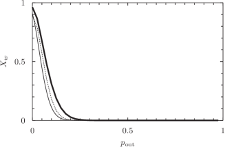
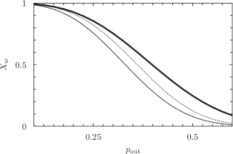
(b) $q=4$ $n=32$ $p_{\mathrm{in}}=.5$	(e) $q=4$ $n=64$ $p_{\mathrm{in}}=.5$
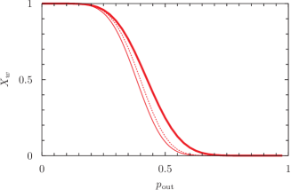
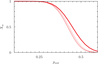
(c) $q=4$ $n=32$ $p_{\mathrm{in}}=.9$	(f) $q=64$ $n=64$ $p_{\mathrm{in}}=.5$

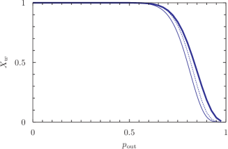
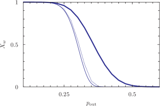
Figure 2: Plots of the fraction $X_{w}$ of well defined nodes [i.e., satisfying Eq. (5)] in the symmetric SBM with $q$ equal size communities each having $n$ nodes as a function of the “noise” $p_{\mathrm{out}}$ (the probability for any given inter-community pair of nodes to be connected by an edge) for different values of $p_{\mathrm{in}}$ (the probability for any given intra-community pair of nodes to be connected by an edge). The different curves provide a comparison between the exact calculation (thick line, Eqs. (6, 7,28)), and independence approximation (thin solid line, Eq. (21)), and independence approximation with normal approximation (dotted line, Eq. (21) with Eq. (17)). We see that the independence approximation is worse for when the number of communities grows large or the number of nodes per community grows small (thick vs thin line). The normal approximation does not significantly affect the accuracy of $X_{w}$ calculation (thin vs dotted line). The region at which $X_{w}\approx 1$ and divergence from $X_{w}=1$ remain fairly well predicted under all approximations.

We now, as promised, turn to the imprecision of the approximation and its origin. The fractions $X_{w,AB}$ are not independent as assumed in Eq. (18). This is so as all $X_{w,AB}$ share the same $\rho_{\mathrm{in}}$. If one particular community $B_{1}$ has a $\rho_{\mathrm{in}}$ higher than $\rho_{\mathrm{out},B_{1}}$, then $\rho_{\mathrm{in}}$ has a greater probability of being larger than the average $\rho_{\mathrm{in}}$. This increases the probability that a future community $B_{i}$ has $\rho_{\mathrm{in}}>\rho_{\mathrm{out},B_{i}}$. Each successive external community which has a lower $\rho_{\mathrm{out}}<\rho_{\mathrm{in}}$ further biases the expected value of $\rho_{\mathrm{in}}$ towards higher values. The overall effect is that $X_{w,A}$ is greater than we find using the independence approximation. Thus, the independence approximation leads in fact to a stringent bound,

$$X_{w}\geq X_{w}^{\mathrm{ind}},$$ (22)

where the equality holds when $q=2$. We will formally derive this bound in section VII. This general bound is vividly illustrated by a simple example. Consider the case of $p_{\mathrm{in}}=p_{\mathrm{out}}$ for equal size communities. If we approximate $n\approx n-1$, each community, including the “in” one, will have equal chances of having the most connections to a given node. Thus, in such a case, $X_{w}$ should equal $1/q$. Using the independence approximation in Eq. (21), however, we will have a $50\%$ probability of well-definedness with respect to each external community, thus leading to the paradoxical results that $X_{w}=\left(\frac{1}{2}\right)^{q-1}$ which is flatly incorrect. Nevertheless, this approximation gives rise to a nontrivial bound of possible analytic utility, which we will improve upon. In the next section, we will compute more rigorous bounds of the fractions of correctly identified nodes in all SBM type partitions. We will then, as promised, illustrate that the independence approximation adheres to the bound of Eq. (22).

VI Fractions of well defined nodes in SBM partitions

To produce an analytical form for the fraction of well defined nodes $X_{w}$, we need to find the probability density of the maximum of a series of random variables. This is a hard task, requiring nested integrals. We can slightly simplify this problem by considering the probability distribution

$$P_{w,A}(\rho_{\mathrm{in}})=P\left[\rho_{\mathrm{in}}>\max\{\rho_{\mathrm{out},B_{1}},\rho_{\mathrm{out},B_{2}},\ldots,\rho_{\mathrm{out},B_{q-1}}\}\right].$$ (23)

Clearly,

$$X_{w,A}(\rho_{\mathrm{in}})=P\left[(\rho_{\mathrm{in}}>\rho_{\mathrm{out},B_{1}})\wedge(\rho_{\mathrm{in}}>\rho_{\mathrm{out},B_{2}})\wedge\ldots\wedge(\rho_{\mathrm{in}}>\rho_{\mathrm{out},B_{q-1}})\right],$$ (24)

with $\wedge$ representing the logical “and”. Thus, to obtain the probability associated with the maximum, we need to integrate the multi-variable probability distribution. In general, of course, there might be states other than a particular planted SBM state for which a high fraction of well-defined nodes are found. Eqs. (23,24) are however independent of any particular particular initial planted state. As we discussed earlier and repeat here, for any node to be well defined in a community (with $B_{1},\cdots,B_{q-1}$ all other external communities), it must have $\rho_{\mathrm{in}}>\max\{\rho_{\mathrm{out},B_{1}},\rho_{\mathrm{out},B_{2}},\ldots,\rho_{\mathrm{out},B_{q-1}}\}$, with $\rho_{\mathrm{in}}$ the associated link density between that node and its proper community (or communities) that, by definition, satisfies this inequality.

We now proceed to re-examine the case of one external community and then illustrate how to properly generalize this result for multiple external communities $\{B_{i}\}_{i=1}^{q-1}$. The probability that $\rho_{\mathrm{out},B_{i}}$ is, for a specific community $B_{i}$, less than $\rho_{\mathrm{in}}$ reads

$$P\left[\rho_{\mathrm{out},B_{i}}<\rho_{\mathrm{in}}\right]=\mathrm{CDF}[\rho_{\mathrm{out},AB_{i}}](\rho_{\mathrm{in}}).$$ (25)

This reduces to Eq. (15) in the Gaussian approximation to the binomial probability distribution function (which we return to more generally below). In Eq. (25), the “$\mathrm{CDF}$” syntax denotes the “Cumulative Distribution Function” of $\rho_{\mathrm{out},AB_{i}}$ which, when the normal approximation to the exact binomial distribution may be invoked, is given by Eqs. (16,17) when these are evaluated at $\rho_{\mathrm{in}}$. Probability density functions and cumulative distribution function nomenclature is reviewed in Appendix A. Generally, we may either employ the $\mathrm{CDF}$ of the normal approximation from Eqs. (10, 11, 15) (whence, as stated above, it reduces to Eqs. (16, 17)) or the exact binomial from the first half of Eqs. (6, 7); the normal $\mathrm{CDF}$ is, of course, a continuous distribution, while the binomial $\mathrm{CDF}$ is a series of discrete steps formed from a sum of discrete quantities. The particular form used for the CDF reduces to an implementation detail of the necessary numerical evaluation. However conceptually both forms (normal or binomial) can be used equivalently with little difference in the results for most graphs (e.g., not exceptionally sparse graphs for which the binomial distribution tends to a Poisson distribution). We now turn to the multi-community case. From Eq. (24),

$$X_{w,A}(\rho_{\mathrm{in}}) = P\left[\rho_{\mathrm{in}}>\rho_{\mathrm{out},B_{1}}\right]P\left[\rho_{\mathrm{in}}>\rho_{\mathrm{out},B_{2}}\right]\ldots P\left[\rho_{\mathrm{in}}>\rho_{\mathrm{out},B_{q-1}}\right],$$ (26)

$$X_{w,A}(\rho_{\mathrm{in}}) = \prod_{i=1}^{q-1}\mathrm{CDF}\left[\rho_{\mathrm{out},B_{i}}\right](\rho_{\mathrm{in}}),$$ (27)

where the product extends over all $q-1$ external communities. The fraction $X_{w,A}$ of nodes which are well-defined is given by $X_{w,A}=P_{w,A}$. Eq. (23) and the results above that followed apply for a given $\rho_{\mathrm{in}}$. To find out the probabilities and fraction of correctly identified nodes, we must integrate over all possible values of $\rho_{\mathrm{in}}$. This leads to

$$X_{w,A}=P_{w,A}=\int_{0}^{1}d\rho_{\mathrm{in}}\mathrm{PDF}\left[\rho_{\mathrm{in},A}\right](\rho_{\mathrm{in}})\prod_{i=1}^{q-1}\mathrm{CDF}\left[\rho_{\mathrm{out},B_{i}}\right](\rho_{\mathrm{in}}).$$ (28)

We may employ the general relation of Eq. (19) to determine the fraction of correctly identified nodes. For equal-size communities, we have

$$X_{w}=\int_{0}^{1}d\rho_{\mathrm{in}}\mathrm{PDF}\left[\rho_{\mathrm{in},A}\right](\rho_{\mathrm{in}})\left(\mathrm{CDF}\left[\rho_{\mathrm{out},B_{i}}\right](\rho_{\mathrm{in}})\right)^{q-1}.$$ (29)

We end up with an integral which can only be easily evaluated for $q=2$. For $q=2$ (and only for $q=2$), we can proceed as in the case of Eq. 16. Note that for $q=2$, the independence approximation is not wrong, as there are no multiple objects to assume independence of (e.g.,trivially, $\left(\frac{1}{2}\right)^{(q-1)}=\frac{1}{q}$ when $q=2$).

That the independence approximation leading to Eq. (21) is not exact for $q>2$ is indeed evident since, as discussed in the example which we just provided earlier, for $p_{\mathrm{in}}=p_{\mathrm{out}}$, the approximation will yield $\left(\frac{1}{2}\right)^{(q-1)}$, while the correct value should approach $\frac{1}{q}$. As $q$ grows larger, the approximation becomes less accurate and the approximation leads to progressively less tight lower bounds on $X_{w}$. Fig. 3 compares brute computation of the well-defined fraction of nodes with our theoretical calculations. We see that the approximations are good as long as the number of communities $q$ is small.

(a) $q=4$ $n=32$ $p_{\mathrm{in}}=.1$	(d) $q=4$ $n=16$ $p_{\mathrm{in}}=.5$
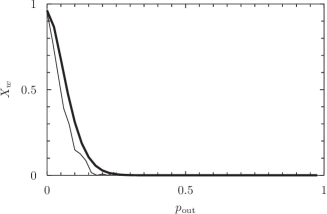
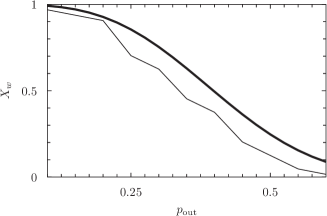
(b) $q=4$ $n=32$ $p_{\mathrm{in}}=.5$	(e) $q=4$ $n=64$ $p_{\mathrm{in}}=.5$
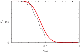
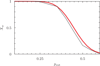
(c) $q=4$ $n=32$ $p_{\mathrm{in}}=.9$	(f) $q=64$ $n=64$ $p_{\mathrm{in}}=.5$

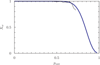
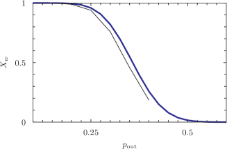
Figure 3: Comparison of exact calculation of well-defined node fraction $X_{w}$ (thick line, Eq. (28, 6, 7)) with brute computation of well-definedness using Eq. (5) from 100 sample graph generations (thin line) of SBM graphs with the given parameters. We see that our theoretical calculations match experimental computation well. However, these results do not consider cascades: all nodes are assumed to stay fixed in their original communities, and well-definedness is calculated relative to that state. The lack of cascades is the reason for a lack of a strict detectability threshold.

In practice, we expect cascade effects: Every misclassified node will influence the number of nodes in each community, thereby affecting the well-definedness of other nodes in those communities. Thus, because of these cascade effects, we expect $X_{w}$ to actually be smaller than even our calculation above, with the greatest accuracy when $X_{w}\approx 1$. The fraction $X_{w}$ is of use in monitoring the performance of community detection algorithms. Fig. 4 compares our calculation of $X_{w}$ to an actual community detection algorithm, and shows that our $X_{w}$ calculation accurately predicts properties of the community detection process which will be elaborated on in future sections.

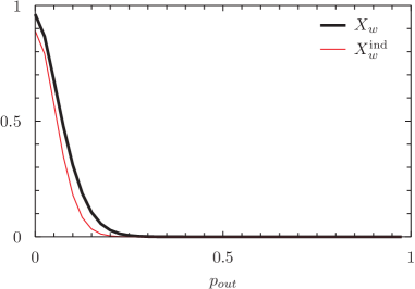
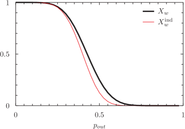
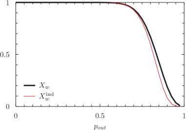
Figure 4: Comparison of different approximations for calculation of $X_{w}$ for a $q=4$ $n=32$ SBM graph at $p_{\mathrm{in}}=\{.1,.5,.9\}$ from top to bottom. The $X_{w}$ calculation (thick line, Eq. (28, 6, 7)) closely matches our independence approximation (thin solid line, Eq. (21)). Furthermore, we see that $X_{w}=1$ accurately predicts the regions at which the absolute Potts model, a recently proposed accurate community detection method, is able to detect communities Ronhovde and Nussinov (2009); Ronhovde and Nussinov (2010). Once $X_{w}<1$, the community detection method rapidly loses accuracy.

VII The independence approximation as an explicit lower bound on general partitions via Jensen’s inequality

Armed with the general expressions for the fraction of correctly identified nodes $X_{w}$, we now return to explicitly demonstrate that the independence approximation leads to explicit bounds of Eq. (22). Within the independence approximation,

$$X_{w}^{\mathrm{ind}}=\left(\int_{0}^{1}d\rho_{\mathrm{in}}\mathrm{PDF}\left[\rho_{\mathrm{in},A}\right](\rho_{\mathrm{in}})\mathrm{CDF}\left[\rho_{\mathrm{out},B_{i}}\right](\rho_{\mathrm{in}})\right)^{q-1}.$$ (30)

Without the independence approximation, we have the result of Eq. (29) which we rewrite here anew for the benefit of the reader to aid comparison,

$$X_{w}=\int_{0}^{1}d\rho_{\mathrm{in}}\mathrm{PDF}\left[\rho_{\mathrm{in},A}\right](\rho_{\mathrm{in}})\left(\mathrm{CDF}\left[\rho_{\mathrm{out},B_{i}}\right](\rho_{\mathrm{in}})\right)^{q-1}.$$ (31)

It is readily seen by Jensen’s inequality Chandler (1987) for convex functions $\varphi$ in its general form as applied to general probability distribution functions ($\int dzf(z)=1$),

$$\varphi\left(\int g(z)f(z)dz\right)\leq\int\varphi\left(g(z)\right)f(z)dz,$$ (32)

for the particular function $\varphi(y)=y^{q-1}$ (with $q\geq 2$), that Eqs. (30, 31) lead to the bound of Eq. (22). An equality always trivially arises when $q=2$ (as is seen from Eq. (32) for $\varphi(y)=y$). We further remark that if, in addition to all possible initially planted SBM partitions, we also examine non SBM type partitions of the original given graphs, the appearance of $X_{w}^{\mathrm{ind}}$ as a lower bound (Eq. (22)) as we derived above by Jensen’s inequality can only be fortified.

VIII Community Detection Thresholds

Thus far, we have focused on the fraction of well defined nodes $X_{w}$. This quantity allows us to know the maximum fraction of nodes any community detection algorithm can achieve. However, it is also useful to have a rough threshold for the case of every node being well-defined. Towards this end, we propose an upper threshold probability

$$X_{w}^{\mathrm{Th,h}}=1-\frac{1}{N}$$ (33)

to test for a proper detection of communities. For $X^{w}$ above $X_{w}^{\mathrm{Th,h}}$, all nodes are well defined a majority of the time. Below $X_{w}^{\mathrm{Th,h}}$, there is a high probability of at least one node not being properly defined in its planted community. At $X_{w}^{\mathrm{Th,h}}$, exactly one node is, on average, mis-grouped. This is the point at which we expect community detection algorithms to no longer perfectly detect communities, and beyond this point to have reduced accuracy. Fig. 5 indicates that this upper threshold somewhat accurately predicts the point at which community detection algorithms begin losing accuracy. For a given $p_{\mathrm{in}}$ value, the $X_{w}^{\mathrm{Th},h}$ threshold occurs at a certain $p_{\mathrm{out}}$ value, which we shall indicate as $p_{\mathrm{out}}^{\mathrm{Th},h}$. This threshold is important for another reason: when $p_{out}<p_{\mathrm{out}}^{\mathrm{Th},h}$, cascade effects where ill-defined and incorrectly detected nodes may influence the detectability of other nodes, are negligble. Thus, when $p_{out}<p_{\mathrm{out}}^{\mathrm{Th},h}$, our calculations are expected to be most accurate, and comparison with detectability is most valid.

At the other extreme, a lower threshold fraction of correctly grouped nodes occurs at the point when the system is entirely decorrelated from its expected community structure, the point at which every node has an equal probability (of size $1/q$) to be found in any community. This threshold fraction is defined by

$$X_{w}^{\mathrm{Th,l}}=\frac{1}{q}+\frac{1}{N}.$$ (34)

We employ a threshold of $1/q+1/N$ instead of simply $1/q$ as $X_{w}$ may never exactly approach the symmetric $1/q$ value for finite size systems. We may mark the corresponding value of $p_{\mathrm{out}}$ with $p_{\mathrm{out}}^{l}$. Without stochastic variance of the edge placement, we would expect $p_{\mathrm{out}}^{l}=p_{\mathrm{in}}$.

By Eq. (22), the results that we arrive at by the independence approximation of Eqs. (18, 21) and, in particular, the corresponding values of the threshold values $p_{\mathrm{out}}^{h,l}$, lead to lower bounds. That is, if we denote by ${p_{\mathrm{out}}^{\mathrm{ind}}}^{h}$ the value of the $p_{\mathrm{out}}$ for which $X_{w}^{\mathrm{ind}}=1-1/N$ and ${p_{\mathrm{out}}^{\mathrm{ind}}}^{h}$ the value of the $p_{\mathrm{out}}$ for which $X_{w}^{\mathrm{ind}}=1/q+1/N$ respectively, then clearly

$$p_{\mathrm{out}}^{h} \geq {p_{\mathrm{out}}^{\mathrm{ind}}}^{h},$$ (35)

$$p_{\mathrm{out}}^{l} \geq {p_{\mathrm{out}}^{\mathrm{ind}}}^{l}.$$ (36)

For $q>2$, the independence approximation leads to an underestimate of the requisite noise to achieve these threshold fraction values of correctly identified nodes; the true critical values of $p_{\mathrm{out}}$ exceeds that found by the independence approximation.

IX The meaning of $X_{w}$ and the role of ill-defined nodes

In order to highlight the importance of fraction of correctly identified nodes $X_{w}$, we regress and note anew how benchmark graphs are typically employed. A planted SBM is constructed and is provided to a solver by solely providing information about all of the edges between nodes that are present in the graph. The solver is not, of course, told which nodes formed the different communities that were used in the construction of the SBM. A good solver is then expected to be able to use only the edge information to recover the planted communities. $X_{w}$ is the fraction of nodes which a method classifies correctly. When $X_{w}=1$, all nodes are, by fiat, properly defined, and reasonable community detection algorithms would be expected to be able to identify the correct community of all nodes. However, when $X_{w}<1$, then there are some nodes which are more strongly connected to a community other than their planted community. In this case, no community detection algorithm should be expected to classify these nodes correctly since the edge structure does not reflect the planted communities. The inability to detect all correct communities might be seen as a flaw in the algorithm, instead of a flaw in the benchmark (the basic premise of our work) as it should be interpreted.

In Fig. 5, we compare the limits of detectability of the absolute Potts model (APM) Ronhovde and Nussinov (2009); Ronhovde and Nussinov (2010) with those derived for general spectral methods Nadakuditi and Newman (2012). We observe that the upper threshold of Eq. (33) fairly accurately predicts both (i) the point at which the fraction of correctly identifiable nodes via spectral-based method (the NN line of Nadakuditi and Newman (2012)) begins decreasing, and (ii) when the APM method ceases to be able to identify communities well. The transitions to the undetectable phase as seen by both methods (i) and (ii) onset at nearly the same value of the noise $p_{\mathrm{out}}$. More interesting, however, is the fact that we see a notable divergence between the ability to detect nodes (as calculated by NN in Nadakuditi and Newman (2012)) and the structure present in the graph. This is true even near our “accurate” range, near the low threshold $p_{\mathrm{out}}^{l}$.

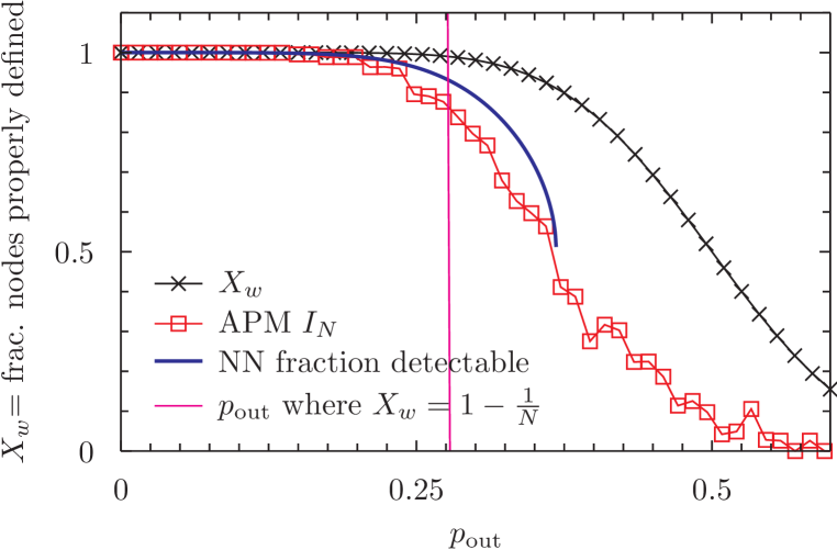
Figure 5: Comparison of $X_{w}$ and actual performance of community detection methods on a stochastic block model with $q=2$, $n=50$, and $p_{\mathrm{in}}=0.5$. We plot $X_{w}$, a upper limit of the fraction of nodes properly classified, with the $X_{w}=1-1/N$ threshold represents the limit of a region where all nodes will be well-defined. We also plot the performance of the absolute Potts model community detection method, and the “optimal” performance of spectral modularity-based methods is also plotted (Eq. (40), Nadakuditi and Newman (2012)). We note a divergence between the theoretical amount of structure available ($X_{w}$) and the performance of community detection methods, even below the $X_{w}=1-1/N$ threshold of all nodes being well-defined.

We can further envision a new experiment to test the reliability of $X_{w}$ in indicating the present graph structure. We construct an SBM graph, and each ill-defined node is shifted to its “correct” community, that community with which it shares the greatest number of edges. (In practice, we use edge density ${\rho_{\mathrm{in}}}_{,C}={k_{\mathrm{in}}}_{,C}/n_{C}$, with $n_{C}$ being the number of nodes in the respective community, as a criteria for shifting). Then, we compare the fraction of properly classified nodes in this “shifted” graph to that in the planted graph. This provides an upper bound of available structure in the graph, if a community detection method knew the original community structure. However, we see (Fig. 6) that there is a significant difference between this measure and our computed fraction $X_{w}$ in the earlier sections (as well as the detectability calculation of Decelle et al. (2011); Nadakuditi and Newman (2012) for which $X_{w}$ is even smaller). This is so as these earlier results concern the structure of the graph (and the ability to infer underlying communities). However, in the shifting process, we begin with the structure and slowly blur it. Consequently, the transition to the disordered structureless phase is not as precipitous. In Fig. 6, we see that $X_{w}$ closely matches the fraction of nodes properly detectable by node-shifting in the high and moderately high $X_{w}$ range. While this process should be considered unreliable for the lower threshold of $X_{w}\approx 1/q$, it demonstrates that our analytic $X_{w}$ calculations do capture some essence of structure available for detection in the graph.

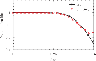
Figure 6: $X_{w}$ compared to a simple node shifting process in a $q=2$ communities, community size $n=50$, $p_{\mathrm{in}}=.5$ SBM averaged over 100 graph instances. Each ill-defined node (in the density formulation, Eq. (5)) is taken and shifted to the community with which it shares the greatest edge density. This process is iteratively repeated until no more changes are possible. We see that $X_{w}$ closely matches this shifting process for moderately high $X_{w}$, indicating that $X_{w}$ does have some relation to embedded graph structure, despite approximations.

X Applicability of results

While the discussion above is focused primarily on equal-sized communities, Eq. (19) generally holds for graphs with communities of any size. However, once we can no longer assume equal size communities, it becomes much more difficult to obtain analytic results. Numerically computing $X_{w}$ is still, however, a relatively simple task. If we go further and allow the coefficients $p_{AB}$ to vary, the form of $X_{w}$ becomes more complex. Nevertheless, for any specific graph instance, an $X_{w}$ value can be calculated by iteration over all nodes and comparing internal and external degree and community sizes.

Our analysis invokes an edge density picture of community detection, where a community of nodes is identified by having more internal edges than external edges to any one other community. On first appearance, this would make it seem that this analysis was specialized to edge-density-based community detection methods. However, given the highly symmetric nature of constant-$n$ stochastic block models, edge density is the only distinguishing factor between communities. There are other competing factors which community detection methods could use in cost functions to judge communities, such as internal edge density, size, number of triangles, and other higher level correlations, with each method weighing these factors differently. However, in SBMs with equal-sized communities $n$, there is only one distinguishing factor: edge density. Thus, all reasonable community detection methods should converge to the same result for this special benchmark class. This rationalizes why various methods such as as those invoking modularity Newman and Girvan (2004), a configuration Potts model by Reichardt and Bornholdt Reichardt and Bornholdt (2006), an Erdős-Rényi Potts model Reichardt and Bornholdt (2004, 2006), its “constant Potts model” extension Traag et al. (2011), and an “absolute” Potts model (no null model definition) Ronhovde and Nussinov (2010) all converge to equivalent cost functions and show equal results in the thermodynamic limit for the constant-$n$ SBM. Thus, Potts-type, and possibly all Decelle et al. (2011); Reichardt and Leone (2008), methods converge to the same result for this special benchmark class. In this sense, our analysis roughly generalizes to all community detection methods on equal size SBM graphs.

XI Algorithmic vs well-definedness crossovers

As alluded to in the Introduction, from a practical vantage point, the detectability limit can also be associated with a phase transition in various cost functions (Potts-type Hamiltonian or other) employed by real algorithms. In the current work, we focused on a related complementary aspect- that of well defined structure that may be probed. Below, we further discuss these.

XI.1 Transitions in algorithmic approaches to community detection

Much previous work, e.g., Hu et al. (2011, 2012a) has shown the existence of several phases in community detection problems and related Hamiltonians. These appear to be bona fide phase transitions as system size grows towards the thermodynamic limit. Similar to other computational problemsMézard et al. (2002), three different phases (marked (i)-(iii) below) are discerned in community detection problems Hu et al. (2011). In (i), the “easy” phase, community detection methods can readily detect proper communities without much effort. (ii) A “hard” phase corresponds to a region where communities exist and are still well-defined yet due to the system complexity an exhaustive sampling is generally required to partition the network. (iii) In the “undetectable” or “unsolvable” phase, no clear community detection is possible regardless of computational effort as the system lacks clear structure. In the spin-glass type “absolute Potts model” approach Hu et al. (2011); Ronhovde and Nussinov (2010); Ronhovde and Nussinov (2009); Hu et al. (2012a, b); Ronhovde et al. (2012a), the transitions between these phases are marked by both thermodynamic (and information theoretic/complexity) measures as well as sharp dynamical spin-glass type signatures. In random graphs, clear spin glass type behavior appears in the hard phase. In the limit of progressively larger number of nodes per community $n$ in power-law graphs, the size of the parameter space region which supported the “hard” phase steadily decreased Hu et al. (2011) suggesting that this phase might disappear in the large $n$ limit. The existence of these phases and their physical content is made visible in some applications such as image segmentation Hu et al. (2012a) and a graph theory based analysis of the structure of glass formers Ronhovde et al. (2011); Ronhovde et al. (2012b). In a companion paper, we illustrate how our edge density based criteria for community detection (in particular that of Eq. (5)) naturally coincide with a general edge density based framework for community detection that includes the absolute Potts model. A mechanical system that can be derived on general graphs which forms a continuous dual to the absolute Potts model exhibits clear transitions into and out of ergodic dynamics Hu et al. (2011) that coincide with the spin-glass type transitions found in the (discrete Potts type) absolute Potts model.

XI.2 Crossovers in “well-definedness” of the planted state

The current work investigates a related complementary problem- the viability of contending underlying ground state (the best community assignments according to a particular CD method) irrespective of how hard it may be to find such a ground state. In particular, we computed bounds of the fraction of well-defined nodes. In a trivial solvable case, $X_{w}$ tends to unity while when the system is maximally disordered this bound veers from above towards $1/q$. These bounds must not be naively confused and equated with transitions appearing in various algorithmic approaches as studied in numerous earlier works. The “well-definedness” that we study in this work conveys information about the defined network structure. When $X_{w}=1$, all nodes are properly defined in their communities and may be accurately placed by an ideal CD algorithm. For large graphs, as $p_{\mathrm{out}}$ is increased, a cross-over occurs into a region where nodes are not well defined according to their intended communities and no method should be able to properly detect all of them beyond the fraction given by $X_{w}$. We now explicitly discuss the behavior as the number of nodes grows large, see Fig. 7 in large dilute graphs ($n\gg 1$ and $k/n\ll 1$). First, we examine the independence approximation of Eq. (18). When the number of nodes per community $n\gg 1$, we may approximate $n\approx n-1$ to obtain

$$P^{\mathrm{ind}}_{w,AB}=\frac{1}{2}\left[1-\mathrm{erf}\left(\frac{p_{\mathrm{out}}-p_{\mathrm{in}}}{\frac{1}{\sqrt{n}}\sqrt{2}\sqrt{p_{\mathrm{in}}(1-p_{\mathrm{in}})+p_{\mathrm{out}}(1-p_{\mathrm{out}})}}\right)\right].$$ (37)

The denominator in this equation provides the width of the erf decay. This denominator decreases as $1/\sqrt{n}$ with increasing community size $n$. Thus, the greater the community sizes, the sharper the crossover between the graph being well defined ($X_{w}\approx 1$) and not ($X_{w}\ll 1$). In the thermodynamic limit of large $n$, a sharp change appears when the parameter $(p_{\mathrm{in}}-p_{\mathrm{out}})=0$. Fig. 7 shows these effects. Using the exact expression of Eq. (28), we see how a finite $n$ crossover becomes progressively sharper as $n$ is increased. Similar arguments will apply to all structural or detectability transitions in graphs. The manifest sharpness that emerges in the large $n$ limit of Eq. (37) as ascertained in the well-definedness of viable ground states goes hand in hand with the different yet complementary bona fide algorithmic thermodynamic phase transition discussed above and in earlier works. In Hu et al. (2011), as $n$ increased a spin-glass type transition emerged in a Potts type algorithm. We remark that in systems with finite $n$ yet divergent $N$, there is only a single undetectable phase Hu et al. (2012b); Ronhovde et al. (2012a).

(a)	(b)

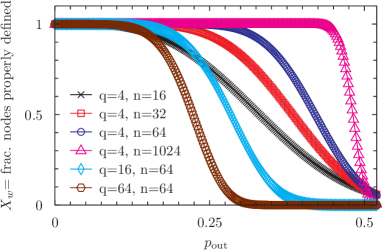
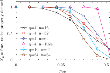
Figure 7: The effects of varying $q$ and $n$ have at constant $p_{\mathrm{in}}=.5$. We see that as $n$ decreases, we get a lower and lower $p_{\mathrm{out}}$ threshold for $X_{w}<1$, the bound for resolving communities. As $q$ increases, our bound decreases. Also, for any given $P_{\mathrm{out}}$, $X_{w}$ is lower for lower $n$ or greater $q$. (a) shows results for our independence approximation, (b) shows results for the correct numerical evaluation. This illustrates how, as the community size $n$ increases, a sharp phase transition between ill-defined and well-defined nodes is approached.

XII Comparison with limits of real community detection algorithms

We now compare our result to the theoretical limit of detectability (DKMZ limit) in the infinite-size limiting caseDecelle et al. (2011); Nadakuditi and Newman (2012). The DKMZ and NN result is in terms of the variables $c_{\mathrm{in}}=Np_{\mathrm{in}}$ and $c_{\mathrm{out}}=Np_{\mathrm{out}}$, and $N=qn$. Translating Eq. (15) of NN Nadakuditi and Newman (2012) for $p_{\mathrm{in}}$ and $p_{\mathrm{out}}$, we have

$$p_{\mathrm{in}}-p_{\mathrm{out}}=\sqrt{\frac{1}{n}\left(p_{\mathrm{in}}+(q-1)p_{\mathrm{out}}\right)}.$$ (38)

It is evident that as $n/q$ becomes large, the right side of this equation approaches zero, forcing $p_{\mathrm{in}}=p_{\mathrm{out}}$ and the results approaches the same limiting case of $p_{\mathrm{in}}>p_{\mathrm{out}}$ for detectability of communities we had in Eq. (1).

Further, NN provide a formula for the fraction of nodes which can be detected in SBMs via spectral-based methodsNadakuditi and Newman (2012). For the $q=2$ case, a pertinent parameter is set by

$$\alpha^{2}=\frac{(c_{\mathrm{in}}-c_{\mathrm{out}})^{2}-2(c_{\mathrm{in}}+c_{\mathrm{out}})}{(c_{\mathrm{in}}-c_{\mathrm{out}})^{2}}.$$ (39)

The fraction $X_{DM}$ (fraction of nodes detected by modularity) of correctly detected vertices using spectral methods that employ the modularity matrix is, according to NN, given by

$$X_{DM}=\frac{1}{2}\left[1+\mathrm{erf}\left(\sqrt{\alpha^{2}/2(1-\alpha^{2})}\right)\right].$$ (40)

We may use the same ideas as in the threshold section (Sec. VIII) to define analogous thresholds

$$X_{DM}^{\mathrm{Th},h}\left(p_{\mathrm{out}}^{DM,h}\right) = 1-\frac{1}{N},$$ (41)

$$X_{DM}^{\mathrm{Th},l}\left(p_{\mathrm{out}}^{DM,l}\right) = \frac{1}{q}+\frac{1}{N}.$$ (42)

In Fig. 8, we observe how the NN fraction of nodes detectable compares with the number of well-defined nodes by our calculations. We see that even in the “accurate” range of our calculations ($X_{w}\approx 1$), there is a significant difference between the amount of present structure ($X_{w}$) and that detectable by modularity ($X_{DM}$). This divergence represents a region where there is nominally structure present, yet this structure cannot be detected.

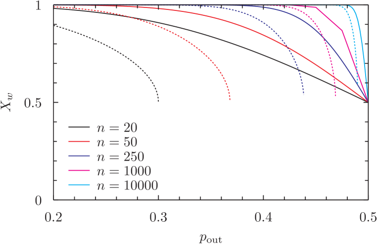
Figure 8: Stochastic block model $q=2$, $p_{\mathrm{in}}=.5$, and varying $n$. Solid lines show $X_{w}$, dotted lines show the modularity-based fraction of nodes identified, with the right endpoints of the lines being the DKMZ limit of detectability. As seen, in the large $n$ limit, the fraction of particles well defined $X_{w}$ and the fraction classifiable via modularity converge. The approach to this limit for small $n$ is different.

XIII “Accurate” methods agree with the $X_{w}$ curve

In earlier sections, we derived a general bound for the fraction of nodes which are properly connected to their communities. We expect any method to be constrained by these bounds. In Fig. 9, we compare various accurate methods to our computed $X_{w}$. As is seen, the fraction of nodes that any method can detect is bounded from above by $X_{w}$. Furthermore, the point at which disparate methods begin losing accuracy is uniformly close to the same value of $p_{out}$ at which $X_{w}$ is only slightly below one. This indicates that, until the first nodes begin being no longer well defined in their communities, it is easy for most methods to accurately detect communities.

We compare the absolute Potts model (“APM” above) Ronhovde and Nussinov (2010) to a method based on desyncronized phase oscillators by Bocaletti et. al. (“OCK-HR”) Boccaletti et al. (2007), Newman’s original modularity optimization algorithm (“Newman 2004 Modularity”) Newman and Girvan (2004), a modularity maximizing simulated annealing approach by Danon et. al. (“Simulated Annealing”) Danon et al. (2005), and a belief propagation and mean field approach by Hastings (“Hastings”) Hastings (2006). These are some of the more common, and more accurate, community detection methods in existence. We compare the experimental results of these methods with our computed $X_{w}$. When $X_{w}$ is high, we observe that the most accurate algorithms are able to almost exactly detect a fraction $X_{w}$ fraction of the nodes. This indicates that not only is $X_{w}$ a bound, but is a fairly complete calculation for the region without cascade effects. When we move to higher $p_{\mathrm{out}}$, our ability to detect communities diverges from the $X_{w}$ theoretical limit. This can be due to cascade effects leading to inaccurate calculation of $X_{w}$, as described in Sec. VI, where each ill-defined node affects more nodes than just itself. Alternatively, the divergence of $X_{w}$ and fractions of nodes detectable, as described in Sec. XII, could also be a cause for this divergence.

(a)

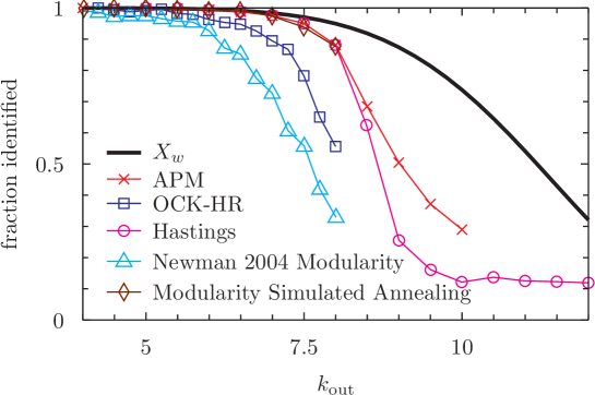
(b) detail of upper region

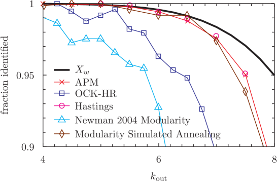
Figure 9: Demonstration of $X_{w}$ representing a limit for “accurate” community detection methods on the $q=4$, $n=32$ SBM graph with $k_{\mathrm{in}}+k_{\mathrm{out}}=16$. We compare a variety of high-accuracy community detection methods (see text), and see that all methods are bound to detect less than $X_{w}$ nodes. Panel (b) is a detail of (a), showing the high $X_{w}$ range. When $X_{w}$ is high, we have minimal cascade effects, and $X_{w}$ is an accurate prediction of the accuracy of the most accurate methods.

XIV General considerations applicable to problems other than the stochastic block model

In what follows, we briefly discuss rather trivial extensions that enable us to compare and extend some considerations to computational/satisfiability problems other than community detection as applied to the stochastic block model. We first express our conditions for well defined community detections as a requirement that a certain cost function vanish. We then further discuss a trivial yet general relation between computational problems with planted solutions and the viability of finding an optimal solution for the computational or satisfiability problems. We finally remark on non-rigorous bounds on the extent of the hard phase in the SBM and possible extensions to other computational problems.

XIV.1 Effective energy

In many computational problems, a certain cost function is to be minimized. All of our analysis thus far has focused on when Eq. (5) may be satisfied. This led to our expressions for the fraction of correctly identified nodes $X_{w}$. We may restate the condition for well defined communities of Eq. (5) by constructing an energy function

$$E=\sum_{A=1}^{q}\sum_{a\in A}\Theta\Big{[}\max_{B\neq A}\left\{\rho_{\mathrm{out},B}^{a}\right\}-\rho_{\mathrm{in}}^{a}\Big{]}.$$ (43)

The above sum is over all communities $A$ and all nodes $a$ within them and $\Theta(x)$ the Heaviside function ($\Theta(x>0)=1$, $\Theta(x<0)=0$). We may now ask whether there exist a partition (or partitions) for which the energy $E=0$. As the energy function of Eq. (43) counts the number of nodes not satisfying our well-defined criteria, we have the correspondence

$$E=N(1-X_{w}).$$ (44)

According to the postulates regarding well-definedness in this work, minimizing this energy corresponds to a rudimentary form of community detection. With the Hamiltonian at hand, we can go beyond an analysis of the system ground states and examine whether it is possible to optimally satisfy the community detection criteria. We can now, as in Hu et al. (2011), broadly define and examine finite temperature entropy, energy, spin-glass type phase transitions that they exhibit, and much more.

XIV.2 Planted states as variational states in general graphs

A trivial yet important point which we wish to emphasize is the following. The planted graph partition might be viewed as a variational state. That is, if the planted partition satisfies Eq. (5) or, correspondingly, is a zero energy (ground state) of the energy function of Eq. (43) then clearly there is at least one state for which Eq. (5) is satisfied. Similarly, if a planted state violates a certain number of conditions of the form of Eq. (5) then there exists at least one partition (i.e., the planted state) which violates the same number of conditions. However, by adjusting the community assignments, we may find a different state (i.e., one which differs from the planted state) which break a smaller number of these conditions and is thus of lower energy. We will denote the fraction of well defined nodes and associated threshold values for this minimal energy state(s) by $\overline{X}_{w}$ and $\overline{p}^{l}$. This is primarily important when we are detecting communities without knowledge of the planted state (i.e., the general practical task of community detection algorithms). In such a case, we search for a state that violates the least number of constraints of the form of Eq. (5) or equivalently has the lowest energy in Eq. (43).

Thus, for any given graph, we will trivially have the inequalities

$$\overline{p}_{\mathrm{out}}^{h} \geq p_{\mathrm{out}}^{h},$$ (45)

$$\overline{p}_{\mathrm{out}}^{l} \geq p_{\mathrm{out}}^{l}.$$ (46)

Similar to Eqs. (33, 34), on the lefthand side of Eq. (46), $\overline{p}_{\mathrm{out}}^{h},\overline{p}_{\mathrm{out}}^{l}$ denote, respectively, values of the noise at which $X_{w}$ is equal to the lower and upper threshold values for the correctly placed nodes relative to the lowest energy state (with no knowledge of a planted state). By contrast, on the righthand side of Eq. (46), $p_{\mathrm{out}}^{h},p_{\mathrm{out}}^{h}$ denote the noise values $p_{out}$ at which the fraction of correctly placed nodes $X_{w}$ achieves lower and upper threshold values relative to a known planted state.

The variational state provided by the planted state, if anything, may lead us to believe that our threshold is smaller than it actually is for finding sensible community partitions. The fact that we detect the lowest-energy ground state, instead of the variational (planted) state, leads us to infer a greater threshold for community detection than we actually have. This may be of utility when the true communities are not known, and the accuracy of the detection must be inferred from the relative noise.

XIV.3 Possible proof of principle on boundaries of hard phase in which problems cannot be easily solvable yet for which contending solutions can be polynomially checked

As is evident from Fig. 5, there is (for general non-vanishing $q/n$ and/or in dense graphs) a finite interval of $p_{out}$ values for which (i) there are on average, as we proved, still meaningful partitions (which can be checked in polynomial time for the conditions specified by Eq. (5)) yet (ii) according to, e.g., Nadakuditi and Newman (2012) there are no spectral algorithms that can efficiently ascertain structure. Together, this suggests as a matter of principle a route for establishing a hard phase as probed by various specific algorithms. The hard phase consists of very challenging graph partitioning problems that cannot be solved efficiently (i.e., may be non-polynomial problems) by any algorithm yet purported solutions can be checked in polynomial time (i.e., belonging to NP). Namely, this situation is one for which the old conjecture $P\neq NP$ may explicitly come to lifeFortnow (2009). We caution that our work (which leads to item(i) above) centered on the use of Eq. (5) while others Decelle et al. (2011); Nadakuditi and Newman (2012); Mossel et al. (2012) did not use these criteria for their point of departure. When satisfied, the criteria of Eq. (5) suggest community structure yet it is possible that non-trivial meaningful clusters can be inferred such that they adhere to other criteria. The rigorous upper bounds that we derived in the current work do not incorporate “cascade effects” (Sec. VI); when these are taken into account, cascade effects may generally lead to lower threshold values of the noise beyond which well defined structure ceases to exist. We reiterate that the cavity-type approximations of DKMZ Decelle et al. (2011) lead to results identical to those of NN as suggested by spectral methods. We should further remark anew that, as illustrated by Mossel et al. (2012), no Bayesian inference algorithm can detect structure beyond for noise values larger the DKMZ expression for the special case of sparse SBM graphs with $q=2$ communities. The general considerations that we invoked here for finding where the hard phase may potentially appear may be replicated to other computational problems.

XV Conclusions

We conclude with a brief synopsis of our results:

$\bullet$ Community detection as a function of graph structure. Detecting communities in general graphs is an NP-type problem that has gained much attention in the last decades. More recently, several groups have examined a particular subclass - the stochastic block model graphs - with the goal of calculating noise thresholds on the ability to detect community structure via various algorithms such as those involving spectral methods or considerations related to the fundamental ability of disparate methods to infer structure. These methods were examined elegantly via the cavity-type approximations and have been bolstered by other considerations. In this work, we take a different path to attack this problem. Specifically, instead of studying limitations of various algorithmic or inference approaches we have turned the problem around and examined the properties of the graph itself to examine to what the community detection partition of the system may have a well-defined solution. This approach enabled us to derive universal bounds independent of any particular community detection algorithm and/or inference methods/approximations. We invoked a simple criterion for community structure that relies on edge densities. Using this, we derived a relationship for the fraction of nodes consistent with the correct community assignment. Our approach is much simpler that of past works and offers a complimentary understanding on the limits of detectability. The ideas introduced in our work, with the principle of focusing on the problem itself, independent of any known algorithms or inference approximations, might have also applications in the analysis of other hard computational problems.

$\bullet$ Rigorous bounds on well-definedness and community detection algorithms. Our bound on the highest number of correctly identifiable vertices of the planted state, in the non-sparse case (such that the exact binomial distribution may be replaced by a normal distibution) is given by $X_{w}(p_{\mathrm{in}},p_{\mathrm{out}},q,n)$ of Eq. (29) (wherein the corresponding CDF is given by Eqs. (16, 17) and the PDF is given by Eq. (10)). We reiterate that this provides a strict upper bound on the accuracy of any community detection method for planted equal community size stochastic block model graphs. For sparse graphs, the exact binomial distribution (or its Poisson distribution approximation) may be invoked in the probability distribution functions. Furthermore, we have derived an “independence approximation” which is most accurate for a small number of communities $q$ or high $X_{w}$. We have shown, by a simple application of Jensen’s inequality, that the independence approximation leads to a strict lower bound on the actual fraction of well defined nodes, $X_{w}^{\mathrm{ind}}\leq X_{w}$. Finally, by comparison with previous accurate community detection algorithms, we have shown that our $X_{w}$ bound is indeed an upper limit for all of these algorithms as is clearly seen in Fig.(9). We achieve the greatest accuracy when $X_{w}$ is high, minimizing cascade effects of ill-definedness. We have established that by focusing on ill-defined nodes and assigning these to the optimal communities, the transition to structureless partitions is no longer as precipitous as it is otherwise. The bounds that we obtain on $X_{w}$ correlate emulates and narrowly lie above the curves found by NN Nadakuditi and Newman (2012) for the fraction of well-defined nodes.

$\bullet$ Sharp behavior in large-size limit. We have demonstrated that as community size $n$ increases, the width of the transition between well-defined and ill-defined decreases. The absolute Potts model approach to community detection problems Ronhovde and Nussinov (2010); Ronhovde and Nussinov (2009) substantiated how the width of intermediate “hard” phase decreases as $n/q$ becomes progressively largerHu et al. (2011, 2012a, 2012b); Ronhovde et al. (2012a) for dilute graphs.

$\bullet$ Difference between solvable problems and checkable solutions. Taken together, the results that we derived in this work for (i) cases when graphs have well defined underlying structure and (iii) earlier results Nadakuditi and Newman (2012); Decelle et al. (2011) concerning the limitations of general spectral algorithms and inference approaches suggest bounds on the hard phase. Within the hard phase, the community detection problem cannot be efficiently solved yet for which purported solutions can be checked in polynomial time. Away from the large $n/q$ limit in dilute graphs the combined results of (i) and (ii) allow for the emergence of polynomially checkable yet extremely hard to solve problems. That is, away from these limits, the hard phase may appear. The surplus of the fraction of well-defined nodes $X_{w}$ that we found in the current work (irrespective of applied algorithm) as compared to the fraction found by the modularity matrix based algorithm of NN Nadakuditi and Newman (2012) is notable. This disparity may highlight difference between solvable problems (NN) and rigorous bounds on proposed contending checkable solutions (the current work) by examining the fraction of nodes that satisfy the criteria for well-definedess.

$\bullet$ Relevance to benchmark graphs. Perhaps the most practical implication of this work relates to the construction and analysis of benchmark graphs for community detection. In order to judge the effectiveness of any algorithm, one must know the expected maximal possible performance. We investigated the performance of various algorithms and examined upper and lower threshold values of noise in stochastic block model graph benchmarks and the role of ill-defined nodes where the community detection criteria are not satisfied. Benchmark graphs such as that of LFR Lancichinetti et al. (2008); Lancichinetti and Fortunato (2009) can be designed to avoid ill-defined nodes by applying a “rewiring” step which keeps internal to external edges at as constant a ratio as possible. In a companion work, we advanced a general edge density based approach to community detection which complements the edge density criteria of Eq. (5) that we invoked in the current workDarst et al. (2013). Aside from examining nodes and their respective edge densities as criteria for stable communities as we have in this work, we may also apply similar criteria to the density of connections between links (i.e., look at a dual graph formed by the vertices placed at the centers of each link of the original graph and ask whether an edge density criterion is satisfied for the edges between these link centers) or connections between triangles, etc. Darst et al. (2013).

Our analysis, while detailed, raises many further questions. Can this analysis be extended to different cost functions, or graphs with power law degree distributions? Can we successfully model cascade effects, where each incorrect nodes affects the size of communities and thus affects more than just itself? Perhaps most importantly, how does this issue intersect with real-world graphs? We hope that in such graphs with real-world planted states, there is some best community definition. Using an analysis similar to the one presented here, to what degree does the graphs edge structure reflects those communities?

In closing, we remark that the analysis we employ here could, potentially, be extended and applied to other random computational problems. In addition to tackling the algorithmic limits of the solution process, our approach enables one to examine said limits from structural standpoint of the problem itself.

Note added in proof: The bulk of this work first appeared in the PhD thesis of one of us (RKD) in October 2012 (available online at Darst (2012)), which extensively studied the issues surrounding ill-defined nodes. We very recently became aware of a related preprint Floretta et al. (2013) which shares some features and a viewpoint similar to our work.

Appendix A Probability distribution nomenclature

Below, for the sake of clarity, we briefly make explicit the very standard shorthand notations of PDF and CDF that we employ. $\mathrm{PDF}\left[\mathbb{X}\right]$ represents the probability density function, the probability of the random variable $\mathbb{X}$ being in the infinitesimal interval $[x,x+dx]$. In Eq. (28), this PDF associated with $\rho_{\mathrm{in},A}$ is given by Eq. (10). Generally, for any distribution, the PDF is given by the respective integral

$$\int_{a}^{b}\mathrm{PDF}\left[\mathbb{X}\right](x)dx=P\left[a\leq\mathbb{X}\leq b\right].$$ (47)

The cumulative distribution function ($\mathrm{CDF}$), for a general distribution function, corresponds to the probability of the random variate $\mathbb{X}$ being less than or equal to a given value,

$$\mathrm{CDF}\left[\mathbb{X}\right](b)=\int_{-\infty}^{b}\mathrm{PDF}\left[\mathbb{X}\right](x)dx=P\left[\mathbb{X}\leq b\right].$$ (48)

For the external links with a PDF given by Eq. (11), the corresponding CDF is [as we stated in the main text] given by Eqs. (16, 17). Both the PDF and CDF may be associated with either the original discrete problem (described by a binomial distribution) or its continuous approximation (a Gaussian as in Eq. (15)), with the corresponding trivial change between integrals to sums in the equations above if the discrete form is sought.

References

- Fortunato (2010) S. Fortunato, Physics Reports 486, 75 (2010), URL http://www.sciencedirect.com/science/article/pii/S03701573090%02841.
- Newman and Girvan (2004) M. Newman and M. Girvan, Physical review E 69, 026113 (2004), URL http://pre.aps.org/abstract/PRE/v69/i2/e026113.
- Darst et al. (2013) R. Darst, D. Reichman, P. Ronhovde, and Z. Nussinov, arXiv preprint arXiv:1301.3120 (2013), URL http://arxiv.org/abs/1301.3120.
- Newman (2006) M. Newman, Proceedings of the National Academy of Sciences 103, 8577 (2006), URL http://www.pnas.org/content/103/23/8577.short.
- Fortunato and Barthelemy (2007) S. Fortunato and M. Barthelemy, Proceedings of the National Academy of Sciences 104, 36 (2007), URL http://www.pnas.org/content/104/1/36.short.
- Lancichinetti and Fortunato (2011) A. Lancichinetti and S. Fortunato, Physical Review E 84, 066122 (2011), URL http://link.aps.org/doi/10.1103/PhysRevE.84.066122.
- Lancichinetti et al. (2008) A. Lancichinetti, S. Fortunato, and F. Radicchi, Physical Review E 78, 046110 (2008), URL http://link.aps.org/doi/10.1103/PhysRevE.78.046110.
- Hu et al. (2011) D. Hu, P. Ronhovde, and Z. Nussinov, Philosophical Magazine 92, 406 (2011), URL http://www.tandfonline.com/doi/abs/10.1080/14786435.2011.6165%47.
- Ronhovde and Nussinov (2009) P. Ronhovde and Z. Nussinov, Physical Review E 80, 016109 (2009), eprint 0812.1072, URL http://link.aps.org/doi/10.1103/PhysRevE.80.016109.
- Decelle et al. (2011) A. Decelle, F. Krzakala, C. Moore, and L. Zdeborová, Physical Review Letters 107, 65701 (2011), URL http://link.aps.org/doi/10.1103/PhysRevLett.107.065701.
- Mossel et al. (2012) E. Mossel, J. Neeman, and A. Sly, Arxiv preprint arXiv:1202.1499 (2012), URL http://arxiv.org/abs/1202.1499.
- Nadakuditi and Newman (2012) R. Nadakuditi and M. Newman, Physical Review Letters 108, 188701 (2012), URL http://link.aps.org/doi/10.1103/PhysRevLett.108.188701.
- McSherry (2001) F. McSherry, in Foundations of Computer Science, 2001. Proceedings. 42nd IEEE Symposium on (IEEE, 2001), pp. 529–537, URL http://ieeexplore.ieee.org/xpls/abs_all.jsp?arnumber=959929&t%ag=1.
- Reichardt and Leone (2008) J. Reichardt and M. Leone, Physical review letters 101, 78701 (2008), URL http://link.aps.org/doi/10.1103/PhysRevLett.101.078701.
- Holland et al. (1983) P. Holland, K. Blackmond, and S. Leinhardt, Social networks 5, 109 (1983), URL http://www.sciencedirect.com/science/article/pii/037887338390%0217.
- Heimlicher et al. (2012) S. Heimlicher, L. Marc, and Massoulié, L., Arxiv preprint arXiv:1209.2910 (2012), URL http://arxiv.org/pdf/1209.2910.pdf.
- Lancichinetti and Fortunato (2009) A. Lancichinetti and S. Fortunato, Phys. Rev. E 80, 016118 (2009), URL http://link.aps.org/doi/10.1103/PhysRevE.80.016118.
- Fortnow (2009) L. Fortnow, Communications of the ACM 52, 78 (2009), URL http://cacm.acm.org/magazines/2009/9/38904-the-status-of-the-%p-versus-np-problem/fulltext.
- Radicchi et al. (2004) F. Radicchi, C. Castellano, F. Cecconi, V. Loreto, and D. Parisi, Proceedings of the National Academy of Sciences of the United States of America 101, 2658 (2004), URL http://www.pnas.org/content/101/9/2658.short.
- Ronhovde and Nussinov (2010) P. Ronhovde and Z. Nussinov, Physical Review E 81, 046114 (2010), URL http://link.aps.org/doi/10.1103/PhysRevE.81.046114.
- Zhang and Zhao (2012) S. Zhang and H. Zhao, Physical Review E 85, 066114 (2012), URL http://link.aps.org/doi/10.1103/PhysRevE.85.066114.
- Zhang et al. (2009) X. Zhang, R. Wang, Y. Wang, J. Wang, Y. Qiu, L. Wang, and L. Chen, EPL (Europhysics Letters) 87, 38002 (2009), URL http://iopscience.iop.org/0295-5075/87/3/38002.
- Brandes et al. (2008) U. Brandes, D. Delling, M. Gaertler, R. Gorke, M. Hoefer, Z. Nikoloski, and D. Wagner, Knowledge and Data Engineering, IEEE Transactions on 20, 172 (2008), URL http://ieeexplore.ieee.org/xpls/abs_all.jsp?arnumber=4358966.
- Brandes et al. (2007) U. Brandes, D. Delling, M. Gaertler, R. Görke, M. Hoefer, Z. Nikoloski, and D. Wagner, in Graph-Theoretic Concepts in Computer Science (Springer, 2007), pp. 121–132, URL http://www.springerlink.com/content/w7p1057m25757210/.
- Chandler (1987) D. Chandler, Introduction to Modern Statistical Mechanics (Oxford, 1987).
- Reichardt and Bornholdt (2006) J. Reichardt and S. Bornholdt, Physical Review E 74, 016110 (2006), URL http://link.aps.org/doi/10.1103/PhysRevE.74.016110.
- Reichardt and Bornholdt (2004) J. Reichardt and S. Bornholdt, Physical Review Letters 93, 218701 (2004), URL http://prl.aps.org/abstract/PRL/v93/i21/e218701.
- Traag et al. (2011) V. Traag, P. Van Dooren, and Y. Nesterov, Physical Review E 84, 016114 (2011), URL http://link.aps.org/doi/10.1103/PhysRevE.84.016114.
- Hu et al. (2012a) D. Hu, P. Ronhovde, and Z. Nussinov, Phys. Rev. E. 85, 016101 (2012a), URL http://link.aps.org/doi/10.1103/PhysRevE.85.016101.
- Mézard et al. (2002) M. Mézard, G. Parisi, and R. Zecchina, Science 297, 812 (2002), URL http://www.sciencemag.org/content/297/5582/812.short.
- Hu et al. (2012b) D. Hu, P. Ronhovde, and Z. Nussinov, Physical Review E 86, 066106 (2012b), URL http://link.aps.org/doi/10.1103/PhysRevE.86.066106.
- Ronhovde et al. (2012a) P. Ronhovde, D. Hu, and Z. Nussinov, EPL (Europhysics Letters) 99, 38006 (2012a), URL http://iopscience.iop.org/0295-5075/99/3/38006.
- Ronhovde et al. (2011) P. Ronhovde, S. Chakrabarty, D. Hu, M. Sahu, K. Sahu, K. Kelton, N. Mauro, and Z. Nussinov, The European Physical Journal E: Soft Matter and Biological Physics 34, 1 (2011), URL http://link.springer.com/article/10.1140/epje/i2011-11105-9.
- Ronhovde et al. (2012b) P. Ronhovde, S. Chakrabarty, D. Hu, M. Sahu, K. Sahu, K. Kelton, N. Mauro, and Z. Nussinov, Scientific reports 2 (2012b), URL http://www.nature.com/srep/2012/120329/srep00329/full/srep003%29.html.
- Danon et al. (2005) L. Danon, A. Diaz-Guilera, J. Duch, and A. Arenas, Journal of Statistical Mechanics: Theory and Experiment 2005, P09008 (2005), URL http://dx.doi.org/10.1088/1742-5468/2005/09/P09008.
- Boccaletti et al. (2007) S. Boccaletti, M. Ivanchenko, V. Latora, A. Pluchino, and A. Rapisarda, Physical Review E 75, 045102 (2007), URL http://link.aps.org/doi/10.1103/PhysRevE.75.045102.
- Hastings (2006) M. Hastings, Phys. Rev. E 74, 035102 (2006), URL http://link.aps.org/doi/10.1103/PhysRevE.74.035102.
- Darst (2012) R. Darst, Ph.D. thesis, Columbia University (2012), URL http://hdl.handle.net/10022/AC:P:14886.
- Floretta et al. (2013) L. Floretta, J. Liechti, A. Flammini, and P. De Los Rios, Arxiv preprint arXiv:1306.2230 (2013), URL http://arxiv.org/abs/1306.2230.