Clues on void evolution II: Measuring density and velocity profiles on SDSS galaxy redshift space distortions

Abstract

Using the redshift-space distortions of void-galaxy cross-correlation function we analyse the dynamics of voids embedded in different environments. We compute the void-galaxy cross-correlation function in the Sloan Digital Sky Survey (SDSS) in terms of distances taken along the line of sight and projected into the sky. We analyse the distortions on the cross-correlation isodensity levels and we find anisotropic isocontours consistent with expansion for large voids with smoothly rising density profiles and collapse for small voids with overdense shells surrounding them. Based on the linear approach of gravitational collapse theory we developed a parametric model of the void-galaxy redshift space cross-correlation function. We show that this model can be used to successfully recover the underlying velocity and density profiles of voids from redshift space samples. By applying this technique to real data, we confirm the twofold nature of void dynamics: large voids typically are in an expansion phase whereas small voids tend to be surrounded by overdense and collapsing regions. These results are obtained from the SDSS spectroscopic galaxy catalogue and also from semi-analytic mock galaxy catalogues, thus supporting the viability of the standard $\Lambda$CDM model to reproduce large scale structure and dynamics.

1 Introduction

Large scale underdensities naturally arise as the result of structure growth. According to our current understanding, the structure of matter evolves from small density fluctuations in the early universe to build up the present day distribution of matter. As the universe evolves, galaxies dissipate from underdense regions and progress towards matter concentrations by the action of gravity, forming both voids and filaments in the process. The void distribution evolves as matter collapses to the structure and galaxies dissipate from voids, making a supercluster-void network (Frisch et al., 1995; Einasto et al., 1997, 2012). This interplay in the formation of voids and structures, allows to think of them as complementary, both encoding useful information to place constraints on the parameters of cosmological models. Hence, while the predominant objects of the large scale galaxy distribution are structures such as groups, clusters, filaments or walls, voids emerge as the relevant features that shape, along with filaments, the structure at the largest scales.

Underdense regions have been identified and analyzed in numerical simulations (Hoffman & Shaham, 1982; Hausman, Olson & Roth, 1983; Fillmore & Goldreich, 1984; Icke, 1984; Bertschinger, 1985; Aragon-Calvo et al., 2010; Aragon-Calvo & Szalay, 2013; Kauffmann & Fairall, 1991) and in galaxy catalogues (Pellegrini, da Costa & de Carvalho, 1989; Slezak, de Lapparent & Bijaoui, 1993; El-Ad & Piran, 1997; El-Ad, Piran & Dacosta, 1997; El-Ad & Piran, 2000; Müller et al., 2000; Plionis & Basilakos, 2002; Hoyle & Vogeley, 2002, 2004; Ceccarelli et al., 2006; Patiri et al., 2006; Neyrinck, 2008) showing similar properties regardless of the details of the identification methods (Colberg et al., 2008) and galaxy sample properties.

Padilla, Ceccarelli & Lambas (2005) show that voids defined by the spatial distribution of haloes and galaxies have similar statistical and dynamical properties. Moreover, the statistics of void and matter distributions are strongly related (White, 1979) and therefore voids are a powerful tool to study the formation and evolution of overdense structures. Since the void population properties are sensitive to the details of structure formation, they can be used to constrain cosmological models (e.g. Peebles, 2001; Park et al., 2012; Kolokotronis, Basilakos & Plionis, 2002; Colberg et al., 2005; Lavaux & Wandelt, 2010; Bos et al., 2012a; Biswas, Alizadeh & Wandelt, 2010; Benson et al., 2003; Park et al., 2012; Bos et al., 2012b; Hernandez-Monteagudo & Smith, 2012; Clampitt, Cai & Li, 2013). Also, due to the global low density environment in which void galaxies are embedded, the galaxy populations in or close to voids are valuable to shed light on the mechanisms of galaxy evolution and its dependence on the large scale environment (Lietzen et al., 2012; Hahn et al., 2007b, a; Ceccarelli et al., 2012; Ceccarelli, Padilla & Lambas, 2008; González & Padilla, 2009).

The simplest approach allows us to characterize individual voids as spherical regions with isotropic motions (Icke, 1984; van de Weygaert & Bertschinger, 1996; Padilla, Ceccarelli & Lambas, 2005; Ceccarelli et al., 2006). However, more detailed analyses suggest that voids are not isolated structures but form part of an intricate network which affects their dynamical properties (Bertschinger, 1985; Melott & Shandarin, 1990; Mathis & White, 2002; Colberg, Krughoff & Connolly, 2005; Shandarin et al., 2006; Platen, van de Weygaert & Jones, 2008; Aragon-Calvo & Szalay, 2013; Patiri, Betancort-Rijo & Prada, 2012).

In a previous work (Ceccarelli et al., 2013, hereafter Paper I), we performed a statistical study of the void phenomenon focussing on void environments. To that end, we examined the distribution of galaxies around voids in the SDSS by computing their integrated density contrast profile. By defining a separation criterion to characterize voids according to their surrounding environment, we obtained two characteristic void types, according to their large-scale radial density profiles: (i) Voids with a density profile indicating an underdense region surrounded by an overdense shell, were dubbed S-Type voids; (ii) voids showing a continuously rising density profiles were defined as R-Type voids. We also found that small voids are more frequently surrounded by overdense shells, and thus they are typically S-type. On the other hand, larger voids are more likely classified as R-Types, i.e., with an increasing integrated density contrast profile, which smoothly rises towards the mean galaxy density. Moreover, this behaviour of SDSS voids results in a correlation between the fraction of voids surrounded by overdense shells and their sizes. This fraction continuously decreases as the void size increases, in a similar way for real, mock and direct numerical simulation samples.

Such a dichotomy in the behaviour of voids was first introduced by Sheth & van de Weygaert (2004), based on an excursion set formalism. The authors classify void profiles and relate them to one of two processes: The void-in-void process describes the evolution of voids that are embedded in larger-scale underdensities. This is the case when small voids merge at an early epoch with other void to form a larger void at a later epoch. On the other hand, underdense regions embedded within larger overdense regions undergo a so-called void-in-cloud process. In a hierarchical structure formation scenario, the filament network subtended by dark matter halos is modified by halo merging. Eventually, some voids located in the interstices of this network will shrink at later times constituting the void-in-cloud scenario. This last case seems to affect more likely small rather than large voids.

Since the evolution of structure in the universe shapes the large scale matter clumps and the voids at the same time, both types of structures are responsive to the details of the contents of the universe, and the equation of state of its constituent species (Einasto et al., 2011). Furthermore, the physics of galaxies in voids is simpler since the non-linear effects of gravity are less significant in regions of space devoid of galaxies. The evolution of void galaxies is affected by the surrounding environment when galaxies are located close to the void edge (Lindner et al., 1996; Ceccarelli et al., 2012). Assuming spherical symmetry, Fillmore & Goldreich (1984) derive similarity solutions to describe the evolution of voids in a perturbed Einstein-de Sitter universe filled with cold, collisionless matter. They suggest, for this simplified model, that different void modes would arise depending on the steepness of the initial density deficit. As a result, the statistics of the void population has been used to constrain parameters of the standard cosmological model (Betancort-Rijo et al., 2009; Biswas, Alizadeh & Wandelt, 2010; Bos et al., 2012a, b), and void catalogues have been exploited to test alternative cosmological models (Biswas & Notari, 2008; Bolejko, Krasiński & Hellaby, 2005; Clampitt, Cai & Li, 2013).

Studies on the dynamics (and evolution) of regions around cosmological voids have been implemented mainly in numerical simulations and semi-analytical galaxies by several authors. For instance, Regos & Geller (1991) have studied the evolution of voids in numerical simulations obtaining the peculiar streaming velocities of void walls. Dubinski et al. (1993) and Padilla, Ceccarelli & Lambas (2005) have analysed the peculiar velocity field surrounding voids in simulations. Also, Sheth & van de Weygaert (2004) and Paranjape, Lam & Sheth (2012) studied the void size evolution in simulations. Aragon-Calvo & Szalay (2013) examined the internal dynamics of voids and their hierarchical features. Albeit, the dynamics of voids have not been extensively studied on observational data. Ceccarelli et al. (2006) used redshift space distortions, peculiar velocities, and a non-linear approximation to determine properties of the peculiar velocity field around voids in the 2dfGRS, including the amplitude of the expansion of voids and the dispersion of galaxies in the directions parallel and perpendicular to the void walls. Patiri, Betancort-Rijo & Prada (2012) suggest the presence of coherent outflows of galaxies in the vicinity of large voids in SDSS.

This paper is organized as follows. In Section 2 we describe the galaxy samples and the corresponding void catalogues. We also describe the semi-analytic mock galaxy samples built from the simulation box. The redshift space distortions on the correlation function are analyzed in Section 3. In Section 4 we present the theoretical approach adopted to model the redshift space distortions from density profiles and velocity flows of galaxies around voids. A comparison of observational results to the numerical simulation and the mock catalogue is given in Section 5, and the results obtained for the observational data are shown in Section 6. Finally, we discuss our results in Section 7.

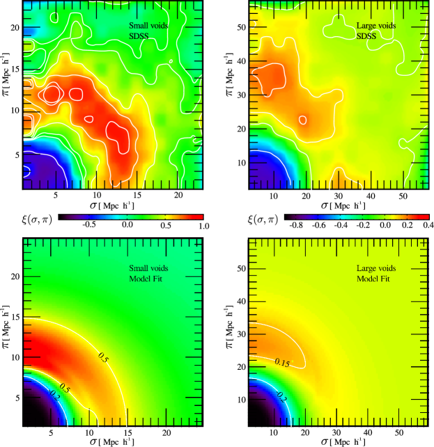
Figure 1: Redshift space distortions of galaxies in the SDSS (upper panels) and the best fit models (bottom panels) for small S-type voids in S1 ($6<\mathrm{R}_{\mathrm{void}}/$h${}^{-1}\,$Mpc$<8$, left panels) and large R-type voids in S3 ($10<\mathrm{R}_{\mathrm{void}}/$h${}^{-1}\,$Mpc$<20$, right panels). The fractions of small R-type voids and large S-type voids are 0.3 and 0.1, respectively. Notice that spatial and color scales change for small and large voids.

2 Data sets

We use the Main Galaxy Sample (Strauss et al., 2002) from the Sloan Digital Sky Survey data release 7 (SDSS-DR7, Abazajian et al., 2009). SDSS photometric data provides CCD imaging data in five photometric bands (UGRIZ, Fukugita et al., 1996; Smith et al., 2002). The SDSS-DR7 spectroscopic catalogue comprises in this release 929,555 galaxies with a limiting magnitude of $r~{}\leq~{}17.77$ mag.

We perform the identification of voids using the algorithm presented by Padilla, Ceccarelli & Lambas (2005) and tested in Ceccarelli et al. (2006). The general properties of the SDSS void sample are introduced in Paper I. Voids in the galaxy distributions are identified over three different volume complete samples, with limiting redshift $0.08$, $0.12$ and $0.15$, whereas corresponding maximum absolute magnitudes in the $r-band$ are $M_{r}=-19.2$, $-20.3$ and $-20.8$, respectively. We denote these three samples as S1, S2 and S3 (see Table 1). In order to compute absolute magnitudes needed in sample definitions, we use the same cosmological parameters than that of the simulation, described later on this Section. The algorithm starts with the identification of the largest spherical regions where the overall density contrast is at most $\delta=-0.9$. The list is cleaned so that each resulting spherical region is not contained in any other sphere satisfying the same condition. The method also avoids the selection of spheres closer than two maximum void radii from the survey boundaries. The centres of underdense spheres are chosen as the locations of void centers, and the scale assigned to each void is the radius of the underdense sphere. It should be noticed that this procedure does not assume that voids are spherical, but ensures that the void is surrounded by a spherical region with overall density below a threshold of $0.1$ times the mean density. Since the resulting void sample depends on the sample dilution (Padilla, Ceccarelli & Lambas, 2005), we seek for the best compromise between the void sample size and the identification confidence, specially for the smallest voids. Therefore, the limiting redshift of the sample is chosen so that a good quality of the void sample is obtained, and also the number of voids remains large enough to achieve statistically significant results. With these criteria, voids down to 5 h${}^{-1}\,$Mpc are well resolved in S1 sample of the catalogue. We obtain 131 voids in this sample with radii ranging from 5 h${}^{-1}\,$Mpc to 22 h${}^{-1}\,$Mpc. The smallest voids are identified in S1, since it has the greater galaxy density. However, due to the limited volume, this sample is not suitable to perform statistical studies of the largest voids, and for this we turn to the additional samples, S2 and S3. The number of voids and the definition of each sample are indicated in Table 1. It can be noticed that the intermediate redshift sample contains a mix of both small and large voids.

In order to test the results, we will implement our method on void samples extracted from a mock galaxy catalogue and from a simulation box. We use galaxies from the semi-analytic model of galaxy formation by Bower, McCarthy & Benson (2008) run on top of the Millennium simulation (Springel et al., 2005; Lemson & Virgo Consortium, 2006). The Millennium cosmological simulation adopts a $\Lambda$CDM cosmological model and follows the evolution of $2160^{3}$ particles, each with 8.6 $\times\,10^{8}\,\mathrm{h}^{-1}M_{\odot}$ in a comoving box of 500 $\mathrm{Mpc}$ a side. The parameters of the model, based on WMAP observations (Spergel et al., 2003) and the 2dF Galaxy Redshift Survey (Colless et al., 2001), are $\Omega_{\Lambda}$ = 0.75, $\Omega_{M}$ = 0.25, $\Omega_{b}$ = 0.045, h = 0.73, n = 1 and $\sigma_{8}$ = 0.9. The semi-analytic model of galaxy formation (GALFORM, Bower, McCarthy & Benson, 2008), generates a population of galaxies within the simulation box, by following the simulated growth of galaxies within dark matter haloes in the simulation. We identified voids in the full simulation box, taking into account the fact that the minimum size of voids that the algorithm is capable of identifing depends on the mean galaxy density (Padilla, Ceccarelli & Lambas, 2005). Accordingly, we imposed a magnitude cut in the sample of semi-analytic galaxies diluting it so that the mean galaxy density is the same than that of the SDSS sample. The semi-analytic galaxy catalogue is found to contain 2534 voids with sizes ranging from 5 to 22 h${}^{-1}\,$Mpc (see Table 1).

The mock catalogue is constructed by reproducing the selection function and angular mask of the SDSS. The resulting semi-analytic galaxy catalogue has similar properties and observational biases to those of the SDSS catalogue. We will use this catalogue in order to calibrate our statistical methods, to interpret the data, and to detect any systematic biases in our procedure. Mainly, we use positions in real space and peculiar velocities of galaxies to test possible projection biases and to quantify the effects of redshift space distortions. The semi-analytic galaxy dataset also provides information on SDSS photometric magnitudes, star formation rates and total stellar masses, based on computations from the semi–analytic model of galaxy formation (Bower, McCarthy & Benson, 2008). The details of the number of R and S-type voids are given in Table 1. Following the same procedure carried out in the SDSS, voids are identified on three volume limited samples, with the same redshift and magnitude thresholds than the used on real data. (i.e. maximum redshift of $0.08$, $0.12$ and $0.15$ and maximum $r-band$ magnitude of $-19.2$, $-20.3$ and $-20.8$, respectively). We denote these three samples as M1, M2 and M3, and comprise 113, 232 and 316 voids, respectively.

From pondering the void radii distributions obtained in each sample we conclude that different samples are more suitable to study voids of different sizes. In the samples with the smallest volumes (S1 and M1) we do not find a significant number of voids with radii larger than 12 h${}^{-1}\,$Mpc. However, a significant number of voids with radii smaller than about 10 h${}^{-1}\,$Mpc are identified, making those samples more suitable for analysing voids of radii between 5 and 10 h${}^{-1}\,$Mpc rather than larger voids. The intermediate volume samples (S2 and M2) reach the maximum number of voids with radii in the range 12–15 h${}^{-1}\,$Mpc. These samples are the most appropriate for studying voids of intermediate size rather than either smaller or larger voids. In the most extensive samples (S3 and M3) we find the largest number of large voids (R_void $>$ 15 h${}^{-1}\,$Mpc) whereas the number of small voids is not adequate for statistical analyses. According to this, we prefer the small volume samples for a detailed statistical study of small voids while large volume samples are used to examine the properties of large voids.

	selection criteria
sample	parent catalogue	limiting magnitude	zlim	NS	NR
S1	SDSS-DR7	-19.2	0.08	48	83
S2	SDSS-DR7	-20.3	0.10	73	174
S3	SDSS-DR7	-20.8	0.12	71	252
M1	mock	-19.2	0.08	48	65
M2	mock	-20.3	0.10	70	162
M3	mock	-20.8	0.12	109	207
	simulation box	-15.9	-	1691	843

Table 1: Galaxy sample selection limits and their corresponding void samples. In all cases we use in void identification volume limited samples, defined by a maximum redshift ($z_{lim}$) and a limiting absolute magnitude in the r-band. The magnitude of galaxies in the mock and simulation box samples correspond to that of the semi-analytic galaxy catalogue. The number of R-type voids (N_R) and S-type voids (N_S) are also indicated.

3 SDSS void galaxy cross-correlation function

In modern spectroscopic galaxy catalogues, redshift measurements are commonly used to estimate galaxy distances. However, these quantities include a contribution from the peculiar velocity component in the line of sight. While this is a drawback when trying to obtain an accurate three-dimensional map of the local universe, dynamical studies can take advantage of the distortions imprinted in redshift space to obtain information about the velocities. In Paper I we have analyzed the large scale environment around voids. We conclude that it is expected that the differences in the spatial distribution of galaxies around voids also manifests as differences in the dynamical properties. Consequently, it is natural to infer that redshift space distortions on the correlation function will show these differences. In this section we search for the dynamics of voids in the redshift space distribution of galaxies around them.

To this end, we measure the void-galaxy cross-correlation function $\xi(\sigma,\pi)$ as a function of the projected ($\sigma$) and line of sight ($\pi$) distances to the void centre. The $\xi(\sigma,\pi)$ function is the excess in the probability of having a galaxy around a given void centre. The standard method to estimate such probability is by counting void-galaxy pairs and normalising by the expected number of pairs for a homogeneous distribution. To compute this normalization it is necessary to produce a random distribution of points with the survey selection function. There are several estimators based on this counting procedure. In this work we have evaluated two of them, the classic estimator (Davis & Peebles, 1983) $\xi=DD/DR-1$, where $DD$ and $DR$ are the numbers of void-galaxy and void-random tracer pair counts respectively, and a symmetric version of the Landy & Szalay (1993) estimator. The latter is computed as $\xi=(DD-DR-RD+RR)/RR$, where in addition to $DD$ and $DR$, we need to calculate $RR$ and $RD$, the numbers of random centre-random tracer and random centre-galaxy pair counts respectively. Since we use volume limited samples of voids the random centre distribution is uniform. We found negligible differences between these two estimators for all void samples. Thus for the sake of simplicity, we perform all the analysis using the Davis & Peebles estimator. The random sample of tracers needed for this estimator was generated following the same procedure described in Paz et al. (2011). Briefly, the expected numerical density of galaxies at a given redshift, with a magnitude below the limit of the survey, is computed from a Schechter luminosity distribution with parameters $\phi_{*}=0.0149\;,M_{*}=-20.44\;,\alpha=-1.05$ (Blanton et al., 2003). The angular selection of the random points consists of a pixel mask based on the SDSSPix software (Swanson et al., 2008). This random catalogue contains about $2\times 10^{7}$ random points (see Paz et al., 2011, for more details).

Without redshift space distortions, $\xi(\sigma,\pi)$ would be isotropic as a function of $\pi$ and $\sigma$. Therefore, any observed anisotropy in the measured $\xi$ function would be evidence of the presence of line-of-sight velocities. Given that these velocities only affect the $\pi$ scale, $\xi$ as a function of $\sigma$, at low $\pi$ values, resembles the real space correlation function. On the other hand, the behaviour of $\xi$ as a function of $\pi$, for low $\sigma$ values, is fully affected by redshift space distortions.

We have defined two types of centre voids depending on their density profiles. Hereby we briefly describe the procedure carried out to define the centre samples; more details can be found in Paper I. The mean integrated density contrast profiles can be defined for $\mathrm{R}_{\mathrm{void}}$ intervals. As shown in Paper I, these average curves have a well defined maximum at a distance $\mathrm{d}_{max}$ from the void centre, except for the largest voids that exhibit an asymptotically increasing profile. We classify voids into two subsamples according to positive or negative values of the integrated density contrast at $\mathrm{d}_{max}$. Voids surrounded by an overdense shell are dubbed S-Type voids, and satisfy $\Delta(\mathrm{d}_{max})>0$. On the other hand R-Type voids are defined as those that satisfy the condition $\Delta(\mathrm{d}_{max})<0$, which corresponds to voids with continuously rising density profiles. This scheme is applied for voids in each of the three volume limited subsamples of the SDSS and mock catalogues, as defined in Section 2, as well as in the semi-analytic sample of galaxies in the simulation box.

In the upper panels of Fig. 1 we show the void-galaxy cross-correlation function of voids in the SDSS. The upper left panel shows the correlation function for the sample of small S-type voids in sample S1. This is representative of small voids since the sample of voids with $\mathrm{R}_{\mathrm{void}}$ in the range 6–8 h${}^{-1}\,$Mpcis dominated by S-type voids (80%). As can be seen in this panel, there is a clear excess in the number counts of void-galaxy pairs at distances larger than $\mathrm{R}_{\mathrm{void}}=8$ h${}^{-1}\,$Mpc(red colours), produced by the characteristic shell of these samples of voids. It can be noticed that there is a compression of the isocorrelation curves in the $\pi$ direction. This is an indication of the mean flow of galaxies towards the void centre.

In the upper right panel we show the correlation function for the sample of large R-type voids in S3. Notice that the spatial and color scales are not the same in each panel to make the variations between each case more clearly visible. As can be seen, the excess of void-galaxy pair counts in the case of small voids at scales 10–15 h${}^{-1}\,$Mpc is not present in the sample of larger voids. Given the trend in the fraction of S-type voids as a function of void radius (reported in Paper I), the sample of large voids is dominated by R-type voids. A continuously rising profile is expected in this case, and indeed it is observed in the $\sigma$ axis at low $\pi$ values. However, as it can be seen in the upper right panel of this figure, an asymmetric structure appears, which is clearly originated on redshift space distortions.

We also show, in the bottom panels of Fig. 1, the synthetic $\xi(\sigma,\pi)$ functions obtained after the application of a model to the corresponding observed functions in the upper panels. We present and describe this model in the following section, where it is used to analyse in more detail the dynamics obtained from redshift distortions.

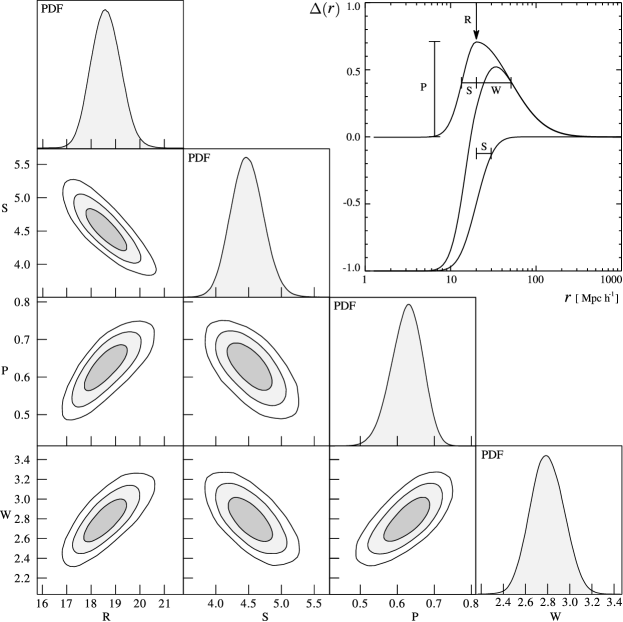
Figure 2: Projections of the Likelihood function for the model applied to intermediate size voids in the mock catalogue. Voids have been identified in the M2 sample of the mock catalogue with radii in the range of 10–12 h${}^{-1}\,$Mpc. The upper-right panel schematically shows the model for the density profiles with a representation of the meaning of each of the parameters in our model.

4 Model for $\xi(\sigma,\pi)$

In the previous section we presented the correlation function obtained from two particularly interesting samples of voids. As has been shown, these samples exhibit different distortion maps. In order to go deeper in the interpretation of such anisotropies, we have implemented a model of the redshift space distortions on the void-galaxy cross-correlation function. Following Peebles (1979) we compute the $\xi(\sigma,\pi)$ function as the convolution of the real space correlation, $\xi(r)$, and the pairwise velocity distribution, $g(\mn@boldsymbol{r},\mn@boldsymbol{w})$:

$$1+\xi(\sigma,\pi)=\int{d^{3}w}\,g(\mn@boldsymbol{r},\mn@boldsymbol{w})\left[1+\xi(r)\right],$$ (1)

where $\mn@boldsymbol{r}\equiv(r_{1},r_{2},r_{3})$ is the real space position of the tracer galaxy with respect to the centre void and $\mn@boldsymbol{w}=\Delta\mn@boldsymbol{v}$ is the velocity of the tracer in the rest frame of the centre object (pairwise velocity). Subscripts denote each of the Cartesian coordinates: the third axis is taken along the line of sight whereas $r_{1}$ and $r_{2}$ are coordinates in the plane of the sky. The redshift space separations of the void-galaxy pair are:

$$\sigma=\sqrt{r_{1}^{2}+r_{2}^{2}}\,\,\,\mathrm{and}\,\,\,\pi=r_{3}+w_{3}/\mathrm{H},$$

which are parallel and perpendicular to plane of the sky, respectively (as defined in the previous section). As mentioned before, the third component of the pairwise velocity ($w_{3}/\mathrm{H}$ in scale units, where H is the Hubble parameter at present time) is the source of the difference between real and redshift space line of sight separations ($r_{3}$ and $\pi$).

In order to compute the redshift space correlation function it is necessary to adopt some prescription for the pairwise velocity distribution, $g$. We assume that this function can be approximated as a Maxwell-Boltzmann distribution centered on a mean velocity field. The latter is a bulk flow given by linear theory, where the mean velocity of the distribution is a function of the density (Peebles, 1976). Since the velocities over the plane of the sky, $w_{1}$ and $w_{2}$, do not affect $\sigma$ or $\pi$ coordinates, the model only requires the definition of the marginal distribution $f$:

$$f\left(w_{3}-\frac{r_{3}}{r}v(r)\right) = \iint dw_{1}\,dw_{2}\,g\left(\mn@boldsymbol{w}-\frac{\mn@boldsymbol{r}}{r}v(r)\right)$$

$$= \frac{1}{\sqrt{2\pi}{\sigma}_{v}}\mathrm{exp}\left(\frac{-\left(w_{3}-v(r)\frac{r_{3}}{r}\right)^{2}}{2{\sigma}_{v}}\right).$$

Finally, the correlation function in redshift space is obtained from

$$1+\xi(\sigma,\pi)=\int{dw_{3}}\frac{1}{\sqrt{2\pi}{\sigma}_{v}}\mathrm{exp}\left(\frac{-\left(w_{3}-v(r)\frac{r_{3}}{r}\right)^{2}}{2{\sigma}_{v}}\right)\left[1+\xi(r)\right],$$ (2)

where $r_{3}=\pi-w_{3}/\mathrm{H}$ and $r^{2}=\sigma^{2}+\left(\pi^{2}-\frac{w_{3}}{\mathrm{H}}\right)^{2}$.

We denote the mass density contrast within a sphere of radius $r$ as $\Delta(r)$. Following Peebles (1976), the mean radial velocity $v(r)$ is related to $\Delta(r)$ by the linear approximation:

$$v(r)\approx-\mathrm{H}r\Delta(r)\frac{\Omega_{m}^{0.6}}{3}.$$ (3)

We have tested other non-linear prescriptions relating $\Delta$ and $v$, given by Yahil (1985) and Croft, Dalton & Efstathiou (1999). However we have not found any significant difference with the linear treatment. This resides in the fact that the density contrast remains small up to large scales in areas around voids.

The integrated density contrast $\Delta(r)$ in a void centered sphere of radius $r$ and volume $V$, is:

$$\Delta(r) = \frac{1}{V}\int_{V}\frac{\rho(r)}{\bar{\rho}}dV-1$$

$$= \frac{3}{r^{3}}\int_{0}^{r}\xi(r)r^{2}dr,$$

where we have used that $\displaystyle\xi(r)=\rho/\bar{\rho}-1$, for a cross–correlation function $\xi(r)$. Then, the real space void-galaxy cross correlation function is related to the density contrast by:

$$\xi(r)=\frac{1}{3r^{2}}\frac{\mathrm{d}}{\mathrm{d}r}\left(r^{3}\Delta(r)\right)\,.$$ (4)

In this framework, given a profile $\Delta(r)$ we can compute the corresponding model for the $\xi(\sigma,\pi)$. However, the estimate of the correlation function using real data (see Section 3) involves the use of a centre void sample. Thus, the profile $\Delta(r)$ should be understood as the mean density profile of the void sample. In order to implement our model on observational data, it is important to select samples of voids which share a similar profile, well represented by the averaged one. In the following subsection, we define a parametric model for this density profile.

4.1 Velocity and density profile model

In order to model the integrated density profiles of voids, we introduce a simple empirical model that contains all the necessary features. The R-type voids (as defined in Section 3) have the simplest profile shapes, a continuously rising curve from zero to the mean density of the universe around the void radius. The error function $\mathrm{erf}(x)$, behaves similarly, therefore we choose this functional form to model such profiles,

$$\Delta_{R}(r)=\frac{1}{2}\left[\mathrm{erf}\left(\mathrm{S}\;\mathrm{log}(r/\mathrm{R})\right)-1\right].$$ (5)

This model depends on two parameters, the void radius R and a steepness coefficient S. On the other hand, the profiles of S-type voids are a bit more complex and require two additional parameters in order to account for the overdensity shell surrounding the void. We add to the rising term in Eq. 5, an additional term representing the peak on density due to this shell. Thus, the overdensity model for S-type void profiles is given by:

$$\Delta_{S}(r)=\frac{1}{2}\left[\mathrm{erf}\left(\mathrm{S}\;\mathrm{log}(r/\mathrm{R})\right)-1\right]+\mathrm{P}\,\mathrm{exp}\left(-\frac{\mathrm{log^{2}}(r/\mathrm{R})}{2\Theta^{2}(r)}\right)$$ (6)

where the Gaussian peak has an asymmetric width,

$$\Theta(r)=\left\{\begin{array}[]{ll}1/\sqrt{2\;\mathrm{S}}&r<\mathrm{R}\\ 1/\sqrt{2\;\mathrm{W}}&r>\mathrm{R}\end{array}\right.$$

As can be seen, such asymmetry is obtained by placing two semi-gaussians instead of just one. This allows us to modify the size of the shell, through the W parameter, without changing the inner shape of the profile, related to S. Therefore, an S-type integrated overdensity profile requires the use of four parameters, namely R, S, P and W. With this profile in equations 3 and 4 it is possible to compute the integral in Eq. 2. In order to perform this integration we use a Runge-Kutta method of sixth order. This allows a robust estimation of the integral avoiding numerical issues related with the rapid variation of the argument function. A schematic view of the role of the parameters on the model is shown in the upper right panel of Fig. 2. The S-type profile (solid line in the upper right panel of Fig. 2) is obtained from the expression 6. The rising term is shown as a long-dashed line, whereas the peak term is represented as short-dashed lines.

4.2 Likelihood sampling and confidence intervals

In the previous subsection we have presented the procedure to compute the model for the redshift space correlation function. In the current subsection we will describe the methods employed to determine the best set of parameters which reproduce a given observed correlation function on real or mock data. To this end we have implemented a Markov Chain Monte Carlo method (hereafter MCMC) to map the likelihood function of the $\xi$ model given the corresponding measurements in a void sample.

The likelihood function compares the modelled correlation functions obtained from different sets of parameters to the measured correlation functions of a given data set, by quantifying the difference between them. The MCMC method samples the posterior probability distribution of the model given the data through a set of markov chains, which traverse the parameter space until they reach the equilibrium distribution. To explore this space, we employ the Metropolis-Hastings algorithm to obtain a random sample of estimates of the model probability. In this process, the likelihood function allows to decide when a given set of parameters is better at describing the observed correlations than a previous set. To properly quantify these model-data distances, we estimate the covariance matrix of the observed correlation function. This matrix plays the role of a metric in the model parameter space. The $\xi(\sigma,\pi)$ function is measured at $15\times 15$ logarithmic bins over the scale intervals used for each sample. Thus, the covariance matrix between each pair of bins in the correlation matrix, hereafter denoted as C, is a squared matrix of $15^{2}\times 15^{2}$ elements. Each element $\mathrm{C}_{ij}$ is the estimator of the variance, computed on the data by jacknife resampling (Tukey, 1958) using the multivariate generalization given by Efron (1987):

$$\mathrm{C}_{ij}=\frac{n-1}{n}\sum_{k=1}^{n}\left[\mathbf{\xi_{(k)}-\xi_{(.)}}\right]_{i}\left[\mathbf{\xi_{(k)}-\xi_{(.)}}\right]_{j}\,,$$ (7)

where $n$ is the number of jackknife realizations, $\mathbf{\xi_{(k)}}$ is the correlation function for the $k$th jackknife realization and $\xi_{(.)}$ is the average of $\mathbf{\xi_{(k)}}$ over the $n$ realizations. The matrix C is not diagonal, since the independence of the correlation values at bins in different scales can not be guaranteed. The probability $\mathscr{L}$ that a given model reproduces the data results is then given by

$$\mathrm{Ln}(\mathscr{L})=-\mathbf{\Delta\xi}\cdot\textbf{{C}}^{-1}\mathbf{\Delta\xi}+\mathrm{const}\,,$$

where $\mathbf{\Delta\xi}$ is a vector containing the differences between the data and modelled correlation functions.

The computation of the likelihood depends on the inverse of the covariance matrix. However, instead of computing $\textbf{{C}}^{-1}$ it is more accurate to solve the system $\textbf{{C}}\mathbf{a}=\mathbf{\Delta\xi}$ for the vector $\mathbf{a}$, obtaining $\mathscr{L}$ as the inner product $\mathbf{a}\cdot\mathbf{\Delta\xi}$. Another numerical issue arises from the fact that the adopted estimator for the covariance gives by definition a positive semidefinite matrix. The covariance matrix takes the form of a sparse matrix, due to fact that the covariance of bin pairs at increasing separations approaches zero, but fluctuates due to the noise introduced by the covariance estimator. This leads, in some cases, to a solution which can be dominated by numerical noise or may even not exist. This issues can be overcome by ”tapering” the covariance matrix, i.e. nullifying the covariance elements at large separations. Following Kaufman (2008), we multiply element-wise the covariance matrix estimated with a correlation matrix, defined to force null values for elements with pair bin distances (calculated in the two dimensions, parallel and perpendicular to the line of sight) larger than 4 bins. The tapering interval of 4 bins is large enough to leave unaltered the principal features of the covariance matrix, ensuring at the same time a positive-definite system. We then compute the probability for any given model in the parameter space using the tapered covariance matrix. This procedure allows us to obtain an estimate of the parameters that maximizes the Likelihood function and its corresponding confidence intervals. We use flat priors for all the parameters in the model, restricting the search in the parameter space to a region where the model gives meaningful profiles.

We show in Fig. 2 an example of the fitting procedure used on a sample of S-type voids taken from the mock catalogue. These voids were identified over the M2 sample of the mock catalogue, with radii ranging from 10 to 12 h${}^{-1}\,$Mpc. The $\xi(\sigma,\pi)$ function was estimated following the methodology described in section 3. In the upper right panel, we schematically represent the parameters involved in the model of the integrated density void profiles $\Delta(r)$, as it is described in the subsection 4.1. We run 40 independent chains to explore this parameter space. The convergence criterion is based on Gelman & Rubin (1992), which compares the spread in the means between chains to the variance of the target distribution. Once a given chain satisfies this criterion, we split it in two parts, discard the first half (ordered by step), and use the rest to map the likelihood function. With this procedure we avoid the early stages of the random walk, where the distribution of points in the parameter space does not necessarily follow the equilibrium distribution. In the diagonal panels of Fig. 2 we show the one-dimensional marginalized constraints over each one of the four parameters (R, S, P, W). We also show the constraints on all pairs of parameters, indicating the 68.3%, 95.5% and 99.7% confidence intervals. As can be seen the marginal distributions for each parameter resemble Gaussian probability densities, thus the uncertainties for each parameter are nearly symmetric. The two dimensional projections of the likelihood function exhibit a well defined maximum, whereas its isoprobability contours indicate that there are not significant degeneracies.

In the bottom panels of Fig. 1, we show two examples of correlation function models obtained from fits run over SDSS results (upper panels). These $\xi(\sigma,\pi)$ functions are obtained from the model with the set of parameters for which the likelihood, with the corresponding correlation measurements, reaches its maximum. As can be seen in a comparison between the upper and lower panels of this figure, the proposed model seems to reproduce the more important features observed in the measured correlations. Moreover, in the lower left panel the white solid line shows two isocorrelation levels ($\xi\approx\,0.5,\,-0.2$) which clearly manifest the expected dynamics for small voids. For instance, the contour corresponding to $\xi\approx-0.2$ reaches the abscissa axis at $\sigma\approx$ 7 h${}^{-1}\,$Mpc, whereas along the $\pi$ direction the contour seems to elongate up to around 8 h${}^{-1}\,$Mpc. This can be thought as a distortion produced in the inner scales of voids by outflow velocities of about 100 $\rm{km~{}s^{-1}}$ h^-1. The opposite behaviour can be seen at the inner part of the isocontour level of $\xi\approx 0.5$. This contour starts at $\sigma\approx$ 11 h${}^{-1}\,$Mpc and reaches the $\pi$ axis at less than 9 h${}^{-1}\,$Mpc. This can be interpreted as a contraction in the correlation function contours due to the presence of redshift distortions, in this case originated by infall velocities around -100 $\rm{km~{}s^{-1}}$ h^-1. This kind of velocity profiles of outflowing velocities inside the void region and infalling velocities at the outskirts, are expected in smaller voids. This is in qualitative agreement with $\Lambda$CDM predictions (see section 1). On the other hand for larger voids, as shown in the lower right panel of Fig. 1, the model exhibits elongated contours in the inner region. More precisely, the inner contour starts at $\sigma\approx 15$ h${}^{-1}\,$Mpcand reaches the $\pi$ axis around 16 h${}^{-1}\,$Mpc. Although the profiles of R-type voids do not reach a maximum at any scales, the modelled $\xi(\sigma,\pi)$ function for this sample exhibits a clear maximum located along the ordinate axis at $\pi\approx$ 27 h${}^{-1}\,$Mpc. This maximum is surrounded by the $\xi\approx 0.15$ contour which encircles a postive correlation region breaking the isotropy of the correlation map. As discussed in section 3 in the case of the observed correlation function (upper right panel in Fig. 1) such anisotropy could be thought as evidence of redshift space distortions at the void outskirts.

In Section 6 we provide an analysis of these results based on the modelled velocity curves, in particular we show in Fig. 4 the corresponding profiles of these two void samples among others. The downward triangles in the left panels of this figure (S-type labeled) correspond to the small S-type voids in the left panels of Fig. 1). The upward triangles in the right panels of Fig. 4 are the derived velocity (upper panel) and density curves (lower panel) from the large R-type voids in the right panels of Fig. 1). For further comments and a more detailed analysis please refer to section 6, where we also analyse the other SDSS void samples shown in the figure.

In this section we have presented an analytic model for redshift space distortions on the void-galaxy cross-correlation function. We showed in this subsection how the parameters of this model can be obtained from fitting the redshift space correlation function. The likelihood and confidence intervals shown in Fig. 2 are a representative example of the results obtained for the different samples used in this work. In the following section we provide an analysis of how well this technique can be used to recover the real velocity and density profile of voids from redshift-space data.

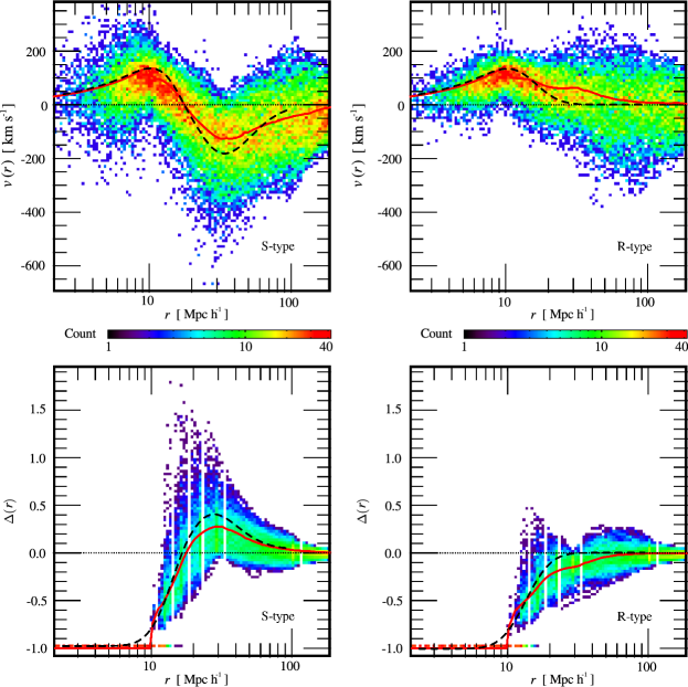
Figure 3: Two–dimensional histograms (color map) of distance-velocity (upper panels) and distance-density (lower panels) void profiles in the semi-analytic sample of galaxies of the simulation box. The color scale displays the number of profiles (integrated density and radial velocity, at lower and upper panels, respectively) overlapping at a given bin in radial distance and velocity or density. Centre voids have been identified in real space with radii in the range 10–12 h${}^{-1}\,$Mpc and separated into S (left) and R-type (right) samples. On each panel, the red solid line shows the averaged values on distance bins of velocity and density. For comparison, we also show the recovered velocity and density curves from the $\xi(\sigma,\pi)$ model in an equivalent mock sample (black dashed line). In this case, voids have been identified in the M2 sample of the mock catalogue with radii in the same range (10–12 h${}^{-1}\,$Mpc).

5 Testing the method on simulations

In the previous section we have presented a parametric model for the $\xi(\sigma,\pi)$ function. We showed the corresponding model results for large and small voids in the SDSS, corresponding to R- and S-types respectively. The model reproduces the main features of the observed redshift space correlation functions for both samples. Also, the model is characterized by a well behaved likelihood function, with not appreciable degeneracies in the parameter space. This suggests that our model not only reproduces the observables but also gives a meaningful set of best-fitting parameters. Given that the model is physically motivated, its results can be used to get insights about the dynamics of the large scale structure around voids. In this section we study the capacity of our model to recover the underlying velocity and density profiles. This analysis is performed by comparing the model results obtained in the mock catalogue with direct measurements of velocity and density profiles in the corresponding simulation. It will also allow us to quantify the effects of observational biases in the results.

In the Fig. 3 we show the results of the proposed test for voids with radii between 10 and 16 h${}^{-1}\,$Mpc. Centre voids have been identified in real space and separated into S (left panels) and R-type (right panels) samples. For each void in the simulation box we measured its radial velocity, $v(r)$, and integrated density profiles, $\Delta(r)$, in spherical shells. We adopt negative values for inward radial velocities, whereas positive values indicate outflowing velocities. In the upper panels of the figure we display the number of radial velocity curves overlapping a given bin in radial distance and radial velocity respecting to the void centre. The spread in radial velocity from void to void at fixed radial distance can be seen from the color map, where redder colours indicate larger number of curves (up to 40). The red solid lines represent the mean velocity profiles for each sample, which are close to the larger concentration of curves, indicating a nearly symmetric spread. We also show, in the bottom panels, the results for the integrated radial density profiles. Here again the color map indicate the number of curves, in this case integrated density profiles, in radial distance and density bins. Red solid lines display the mean density curves for each sample (S and R-type voids at left and right panels, respectively). Finally, we compare these simulation results with those estimated by using our model in redshift space data. We show, with dashed black lines, the velocity and density profile estimates obtained by applying our model in the mock catalogue, following the procedure described in Section 4. In synthesis, for S and R-type voids in the M2, we compute the redshift space void-galaxy correlation function, $\xi(\sigma,\pi)$, and its corresponding model fits.

As can be seen, for both velocity and density profiles the fitting procedure is successful in recovering the underlying behaviour in the simulation. Some differences can be seen at separations larger than the void radius and are due to the limitation of the model for the density profile to reproduce the detailed shape of the actual profile. This of course translates into some difficulty in reproducing the velocity profiles. However, the overdensity values and the mean velocity differences are smaller than $0.3$ and 100 $\rm{km~{}s^{-1}}$ respectively, and the model successfully recovers the S- or R-type nature of the profiles in both density and velocity. In the following section we will apply this procedure to SDSS voids.

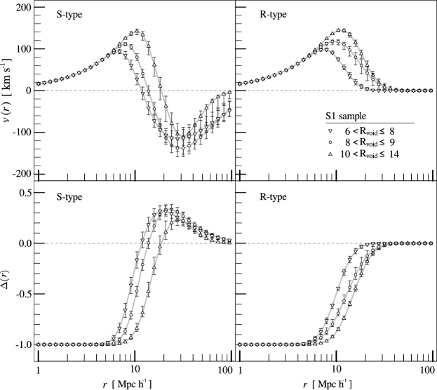
Figure 4: Void–centric radial galaxy density profiles $\Delta(r)$ (lower panels) and void–centric radial galaxy velocity profiles (upper panels) for S-type (left) and R-type (right) voids in the S1 sample. Different void radii ranges are indicated with downward triangles (6–8 h${}^{-1}\,$Mpc), circles (8–9 h${}^{-1}\,$Mpc) and upward triangles (10–14 h${}^{-1}\,$Mpc). Error bars indicate the region enclosing all curves within 68.3% uncertainty in parameter space.

sample	rmin	rmax	type	R	S	P	W
S1	6	8	R	10.06$\pm$ 0.06	5.1 $\pm$ 0.3	-	-
			S	11.0$\pm$ 0.3	5.7 $\pm$ 0.3	0.42 $\pm$ 0.03	1.77 $\pm$ 0.09
	8	9	R	12.8$\pm$ 0.3	3.9 $\pm$ 0.3	-	-
			S	13.4$\pm$ 0.4	5.5 $\pm$ 0.3	0.46 $\pm$ 0.04	2.0 $\pm$ 0.1
	10	14	R	15.0$\pm$ 0.2	4.6 $\pm$ 0.2	-	-
			S	18.5$\pm$ 0.9	4.8 $\pm$ 0.4	0.58 $\pm$ 0.04	2.7 $\pm$ 0.1
S2	9	12	R	13.5 $\pm$ 0.2	5.0 $\pm$ 0.2	-	-
			S	15.1 $\pm$ 0.4	4.9 $\pm$ 0.2	0.39 $\pm$ 0.03	1.83 $\pm$ 0.09
	12	15	R	16.5 $\pm$ 0.2	4.8 $\pm$ 0.1	-	-
			S	17.7 $\pm$ 0.4	6.1 $\pm$ 0.3	0.32 $\pm$ 0.03	1.7 $\pm$ 0.1
	15	25	R	22.4 $\pm$ 0.3	4.0 $\pm$ 0.1	-	-
S3	11	14	R	14.5 $\pm$ 0.1	4.9 $\pm$ 0.1	-	-
			S	17.0 $\pm$ 0.2	5.4 $\pm$ 0.2	0.43 $\pm$ 0.02	2.05 $\pm$ 0.07
	14	19	R	17.6 $\pm$ 0.1	4.3 $\pm$ 0.1	-	-
	19	26	R	25.5 $\pm$ 0.1	4.01 $\pm$ 0.09	-	-

Table 2: Model parameters (see Eqs. 5, 6 and 4.1) obtained for the different subsamples of SDSS voids. Minimum and maximum radii ($r_{min}$ and $r_{max}$, respectively) are expressed in units of h${}^{-1}\,$Mpc.

6 SDSS results

The large–scale region around voids determines two different populations of voids. This was predicted from theoretical considerations in Sheth & van de Weygaert (2004), who also found that void environments are a key factor in their dynamical behaviour. In Paper I we found that small voids are likely to be surrounded by overdense shells, whereas larger voids tend to show smoothly rising profiles. According to the previously mentioned results, a different dynamical behaviour of S and R-type voids is expected. This has been studied for samples of voids derived from numerical simulations, both in the full simulation box and in mock catalogues (including Paper I). However, the corresponding analysis in observational samples has not yet been carried out, and this paper aims at confronting the observations to the theoretical model expectations. Thus, we have applied the methods described in Section 3 to our void catalogues in SDSS.

In the lower panels of Fig. 4 we show the resulting void–centric radial galaxy density profiles, $\Delta(r)$, for S-type (left) and R-type (right) voids in sample S1. The upper panels show the corresponding void–centric radial galaxy velocity profiles. As is indicated in the figure, the different symbols correspond to different ranges in void sizes. We indicate with downward triangles the void radii in the range 6–8 h${}^{-1}\,$Mpc, with circles voids with radii in the range 8–9 h${}^{-1}\,$Mpc; and with triangles voids with radii in the range 10–14 h${}^{-1}\,$Mpc. The error bars in Fig. 4 represent the 68.3% uncertainties resulting from the MCMC likelihood mapping. As it can be seen in the figure the modelled profiles of S and R-type voids are satisfactorily recovered and describe the typical behaviour of the two types of voids. Indeed, the observed density profiles are consistent with the modelled profiles within uncertainties (not shown for the sake of simplicity). Regarding the velocity profiles (upper panels of Fig. 4), it can be seen that the S-type voids show two different dynamical regimes. While inner regions are in expansion, the large–scale void walls are collapsing. This is in agreement with the void–in–cloud scenario introduced by Sheth & van de Weygaert (2004) and the direct measurements in our numerical simulations presented in Paper I. On the other hand, the fitted velocity profiles of R-type voids never exhibit infall velocities as can be seen in the bottom-right panel if this figure. This behaviour fits well with the void-in-void scheme, which indicates that voids embedded in low density large–scale regions are likely to be expanding. These results provide the first observational evidence of the two processes involved in void evolution. We also find that the behaviour of these profiles are different as the void size increases. Where voids surrounded by overdense large–scale shells are under contraction, voids laking this outer overdensity are usually expanding. In this scenario, voids embedded in overdense environments are dominated by gravitational collapse rather than by expansion. Consequently, it is likely that many of the small voids with a surrounding overdense shell have sank inward by the present epoch. Larger voids, on the other hand, are probably expanding in concordance with the formation of the large structures that shape them.

We applied this procedure to the R and S-type subsamples in SDSS and mock catalogues described in Table 1. In the Table 2 we show the resulting model parameter fits, along with their uncertainties, derived from each subsample. The radii ranges have been chosen taken into account the distribution of void radii, so that the sample is in each case divided into three subsamples with nearly the same number of voids each. As can be appreciated in this table, the parameter values support the scenario of a dichotomy in void evolution.

7 Summary and conclusions

We have performed a statistical study of the void phenomenon focussing on the dynamics of the surrounding regions of voids. We used samples of voids identified following the procedure described in Padilla, Ceccarelli & Lambas (2005). We constructed catalogues of voids in the SDSS-DR7, as well as in mock catalogues and in the parent simulation box to test the effects of observational biases.

We analyze the dynamics of voids with and without a surrounding overdense shell in the SDSS, dubbed R-type and S-type respectively, following Paper I. We find that small voids, which are more frequently surrounded by overdense shells (see Paper I), are likely to be in a collapse stage. On the other hand larger voids are in expansion, due to they have a large fraction of R-type profiles (Paper I). Using a model based on the linear theory of gravitational collapse, we model the void-galaxy cross-correlation function in redshift space to take advantage of the redshift-space distortions to obtain the dynamical properties of galaxies around voids. The analysis of the mock catalogues shows that the model successfully recovers the underlying velocity and density profiles of voids from redshift space samples. When applying this procedure to SDSS data, we obtained evidence of a twofold population of voids according to their dynamical properties as suggested on previous observational studies (Paper I) and as predicted by theoretical considerations by Sheth & van de Weygaert (2004). According to this, some voids show a continuously rising profile fitting within the void-in-void scheme proposed by Sheth & van de Weygaert (2004). Our redshift space-distortion studies indicate that this type of voids are likely to be expanding. Small voids, on the other hand, are tipically surrounded by an overdense shell and their redshift space distortions indicate that they are more likely to be collapsing.

We test and interpret our results by comparing SDSS results to a semi-analytic mock galaxy catalogue extracted from the Millennium simulation. Both the mock catalog and the observational results are in very good agreement, providing additional support to the viability of a $\Lambda$CDM model to reproduce the large scale structure of the Universe as defined by the void network and their dynamics.

References

- Abazajian et al. (2009) Abazajian K. N. et al., 2009, ApJSS, 182, 543
- Aragon-Calvo & Szalay (2013) Aragon-Calvo M. A., Szalay A. S., 2013, MNRAS, 428, 3409
- Aragon-Calvo et al. (2010) Aragon-Calvo M. A., van de Weygaert R., Araya-Melo P. A., Platen E., Szalay A. S., 2010, MNRAS, 404, L89
- Benson et al. (2003) Benson A. J., Hoyle F., Torres F., Vogeley M. S., 2003, MNRAS, 340, 160
- Bertschinger (1985) Bertschinger E., 1985, ApJS, 58, 1
- Betancort-Rijo et al. (2009) Betancort-Rijo J., Patiri S. G., Prada F., Romano A. E., 2009, MNRAS, 400, 1835
- Biswas, Alizadeh & Wandelt (2010) Biswas R., Alizadeh E., Wandelt B. D., 2010, Physical Review D, 82, 23002
- Biswas & Notari (2008) Biswas T., Notari A., 2008, 06, 021
- Blanton et al. (2003) Blanton M. R. et al., 2003, ApJ, 592, 819
- Bolejko, Krasiński & Hellaby (2005) Bolejko K., Krasiński A., Hellaby C., 2005, MNRAS, 362, 213
- Bos et al. (2012a) Bos E. G. P., van de Weygaert R., Dolag K., Pettorino V., 2012a, MNRAS, 426, 440
- Bos et al. (2012b) Bos E. G. P., van de Weygaert R., Ruwen J., Dolag K., Pettorino V., 2012b, preprint (arXiv:1211.3249)
- Bower, McCarthy & Benson (2008) Bower R. G., McCarthy I. G., Benson A. J., 2008, MNRAS, 390, 1399
- Ceccarelli et al. (2012) Ceccarelli L., Herrera-Camus R., Lambas D. G., Galaz G., Padilla N. D., 2012, MNRAS, 426, L6
- Ceccarelli, Padilla & Lambas (2008) Ceccarelli L., Padilla N., Lambas D. G., 2008, MNRAS, 390, L9
- Ceccarelli et al. (2006) Ceccarelli L., Padilla N. D., Valotto C., Lambas D. G., 2006, MNRAS, 373, 1440
- Ceccarelli et al. (2013) Ceccarelli L., Paz D., Lares M., Padilla N., Lambas D., 2013
- Clampitt, Cai & Li (2013) Clampitt J., Cai Y.-C., Li B., 2013, MNRAS, 431, 749
- Colberg, Krughoff & Connolly (2005) Colberg J. M., Krughoff K. S., Connolly A. J., 2005, MNRAS, 359, 272
- Colberg et al. (2008) Colberg J. M. et al., 2008, MNRAS, 387, 933
- Colberg et al. (2005) Colberg J. M., Sheth R. K., Diaferio A., Gao L., Yoshida N., 2005, MNRAS, 360, 216
- Colless et al. (2001) Colless M. et al., 2001, MNRAS, 328, 1039–1063
- Croft, Dalton & Efstathiou (1999) Croft R. A. C., Dalton G. B., Efstathiou G., 1999, MNRAS, 305, 547
- Davis & Peebles (1983) Davis M., Peebles P. J. E., 1983, ApJ, 267, 465
- Dubinski et al. (1993) Dubinski J., da Costa L. N., Goldwirth D. S., Lecar M., Piran T., 1993, ApJ, 410, 458
- Efron (1987) Efron B., 1987, The Jackknife, the Bootstrap, and Other Resampling Plans (CBMS-NSF Regional Conference Series in Applied Mathematics). Society for Industrial Mathematics
- Einasto et al. (2011) Einasto J. et al., 2011, A&A, 534, 128
- Einasto et al. (2012) Einasto M. et al., 2012, A&A, 542, 36
- Einasto et al. (1997) Einasto M., Tago E., Jaaniste J., Einasto J., Andernach H., 1997, A&AS, 123, 119
- El-Ad & Piran (1997) El-Ad H., Piran T., 1997, ApJ, 491, 421
- El-Ad & Piran (2000) El-Ad H., Piran T., 2000, MNRAS, 313, 553
- El-Ad, Piran & Dacosta (1997) El-Ad H., Piran T., Dacosta L. N., 1997, MNRAS, 287, 790
- Fillmore & Goldreich (1984) Fillmore J. A., Goldreich P., 1984, ApJ, 281, 9
- Frisch et al. (1995) Frisch P., Einasto J., Einasto M., Freudling W., Fricke K. J., Gramann M., Saar V., Toomet O., 1995, A&A, 296, 611
- Fukugita et al. (1996) Fukugita M., Ichikawa T., Gunn J. E., Doi M., Shimasaku K., Schneider D. P., 1996, AJ, 111, 1748
- Gelman & Rubin (1992) Gelman A., Rubin D. B., 1992, Statist. Sci., 7, 457
- González & Padilla (2009) González R. E., Padilla N. D., 2009, MNRAS, 397, 1498
- Hahn et al. (2007a) Hahn O., Carollo C. M., Porciani C., Dekel A., 2007a, MNRAS, 381, 41
- Hahn et al. (2007b) Hahn O., Porciani C., Carollo C. M., Dekel A., 2007b, MNRAS, 375, 489
- Hausman, Olson & Roth (1983) Hausman M. A., Olson D. W., Roth B. D., 1983, ApJ, 270, 351
- Hernandez-Monteagudo & Smith (2012) Hernandez-Monteagudo C., Smith R. E., 2012, preprint (ArXiv 1212.1174)
- Hoffman & Shaham (1982) Hoffman Y., Shaham J., 1982, ApJL, 262, L23
- Hoyle & Vogeley (2002) Hoyle F., Vogeley M. S., 2002, ApJ, 566, 641
- Hoyle & Vogeley (2004) Hoyle F., Vogeley M. S., 2004, ApJ, 607, 751
- Icke (1984) Icke V., 1984, MNRAS, 206, 1P
- Kauffmann & Fairall (1991) Kauffmann G., Fairall A. P., 1991, MNRAS, 248, 313
- Kaufman (2008) Kaufman C., 2008, J. Am. Statist. Assoc., 1545–1555
- Kolokotronis, Basilakos & Plionis (2002) Kolokotronis V., Basilakos S., Plionis M., 2002, MNRAS, 331, 1020
- Landy & Szalay (1993) Landy S. D., Szalay A. S., 1993, ApJ, 412, 64
- Lavaux & Wandelt (2010) Lavaux G., Wandelt B. D., 2010, MNRAS, 403, 1392
- Lemson & Virgo Consortium (2006) Lemson G., Virgo Consortium t., 2006, preprint (astro-ph/0608019)
- Lietzen et al. (2012) Lietzen H., Tempel E., Heinämäki P., Nurmi P., Einasto M., Saar E., 2012, A&A, 545, 104
- Lindner et al. (1996) Lindner U. et al., 1996, A&A, 314, 1
- Mathis & White (2002) Mathis H., White S. D. M., 2002, MNRAS, 337, 1193
- Melott & Shandarin (1990) Melott A. L., Shandarin S. F., 1990, Nat., 346, 633
- Müller et al. (2000) Müller V., Arbabi-Bidgoli S., Einasto J., Tucker D., 2000, MNRAS, 318, 280
- Neyrinck (2008) Neyrinck M. C., 2008, MNRAS, 386, 2101