Neutrino Mixing and Masses from a Minimum Principle

Abstract

We analyze the structure of quark and lepton mass matrices under the hypothesis that they are determined from a minimum principle applied to a generic potential invariant under the $\left[SU(3)\right]^{5}\otimes{\mathcal{O}}(3)$ flavor symmetry, acting on Standard Model fermions and right-handed neutrinos. Unlike the quark case, we show that hierarchical masses for charged leptons are naturally accompanied by degenerate Majorana neutrinos with one mixing angle close to maximal, a second potentially large, a third one necessarily small, and one maximal relative Majorana phase. Adding small perturbations the predicted structure for the neutrino mass matrix is in excellent agreement with present observations and could be tested in the near future via neutrino-less double beta decay and cosmological measurements. The generalization of these results to arbitrary sew-saw models is also discussed.

PACS: 11.30.Hv, 12.15.Ff

1 Introduction

The gauge interactions of the Standard Model (SM) admit a large, global, flavor symmetry. Matter fields in the SM are described by quark and lepton doublets, $q_{L}$ and $\ell_{L}$, and by right-handed singlets corresponding to $up$ and $down$ quarks and to electron-like leptons: $U_{R}$, $D_{R}$, $E_{R}$. With three quark and lepton generations, massless neutrinos, and omitting $U(1)$ factors unessential to the present work, the flavor group is Chivukula:1987py :

$${\cal G}_{0}=\left[SU(3)\right]^{5}=SU(3)_{q}\otimes SU(3)_{U}\otimes SU(3)_{D}\otimes SU(3)_{{\ell}}\otimes SU(3)_{E}\,.$$ (1)

Masses for the observed neutrinos can be generated with the see-saw mechanism Minkowski:1977sc , by introducing at least two generations of additional Majorana neutrinos, $N_{i}$. The latter are endowed with a Majorana mass matrix with possibly large eigenvalues, and coupled to the lepton doublets by Yukawa interactions. In analogy with the quark sector, here we assume three Majorana generations. We also assume the maximal flavor symmetry acting on the $N_{i}$ in the limit of vanishing Yukawa couplings but non-vanishing Majorana masses, i.e. ${\cal O}(3)$. The flavor group for this case is Cirigliano:2005ck :

$${\cal G}=\left[SU(3)\right]^{5}\otimes{\mathcal{O}}(3)\,.$$ (2)

The large flavor group in Eq. (2), of course, does not correspond to observed symmetries. In the SM, global symmetries are explicitly broken by the Yukawa couplings of matter fields to the $SU(2)_{L}$ scalar doublet, whose vacuum expectation value (vev) is responsible for the spontaneous breaking of the $SU(2)_{L}\otimes U(1)$ gauge symmetry Englert:1964et .

Explicit breaking avoids the presence of unseen Goldstone or pseudo Goldstone bosons with the disadvantage, however, that values and textures of the Yukawa coupling matrices are out of reach of any theoretical consideration. Also, this picture presents the danger that any new physics will bring in new independent amplitudes to Flavor Changing Neutral Current (FCNC) processes, spoiling the extremely good SM predictions, see e.g. Ref. Isidori:2010kg . This can be avoided by the so called Minimal Flavor Violation (MFV) principle D'Ambrosio:2002ex , the statement that in any new physics sector the only sources of flavor symmetry breaking accessible at low energies are the same Yukawa couplings. Even the MFV principle, however, does not provide an explanation of the observed pattern of masses and mixings of quarks and leptons.

In this paper we want to discuss a different option, namely that the Yukawa couplings are the vacuum expectation values of Yukawa fields, to be determined by a minimum principle applied to some potential, $V({\it Y})$, invariant under the full flavor group ${\cal G}$. In this case, one may use group theoretical methods to identify the natural extrema and characterize the texture of the resulting Yukawa matrices.

The simplest realization of the idea of a dynamical character for the Yukawa couplings is to assume that

$${\it Y}=\frac{\langle 0|\Phi|0\rangle}{\Lambda}$$ (3)

with $\Lambda$ some high energy scale and $\Phi$ a set of scalar fields with transformation properties such as to make invariant the effective Lagrangians and the potential $V({\it Y})$ under $\cal G$. To avoid the problem of unseen Goldstone bosons, ${\cal G}$ may be in fact a local gauge symmetry broken at the scale $\Lambda$, with an appropriate Higgs mechanism, see e.g. Ref. Grinstein:2010ve .

The idea that quark masses could arise from the minimum of a chiral $SU(3)\otimes SU(3)$ symmetric potential was considered in the sixties by N. Cabibbo, in the attempt to determine theoretically the value of the Cabibbo angle, and group theoretical methods were established in Refs. Michel:1970mua and Cabibbo:1970rza to identify the natural extrema of the potential. Further attempts towards a dynamical origin of the Yukawa couplings, employing either $G_{0}$ or other flavor groups and different flavor-breaking fields, have been proposed in Refs. Froggatt:1978nt ; Anselm:1996jm ; Barbieri:1999km ; Berezhiani:2001mh ; Harrison:2005dj ; Feldmann:2009dc ; Alonso:2011yg ; Nardi:2011st ; Alonso:2012fy ; Espinosa:2012uu ; Alonso:2013mca . In all cases, the analysis reduces to determining the possible invariants made out of Yukawa fields, and explore their extrema.

In this paper, we apply the theoretical considerations devised in Refs. Michel:1970mua ; Cabibbo:1970rza for chiral symmetry, to the flavor group ${\cal G}$ in Eq. (2). Interestingly, we find different textures for the Yukawa matrices of quarks and leptons. For quarks, we find the hierarchical mass pattern of the third vs the first two generations and unity Cabibbo-Kobayashi-Maskawa (CKM) matrix. However, for leptons, hierarchical masses for charged leptons are accompanied by degenerate Majorana neutrinos with one, potentially two, large mixing angles and one maximal relative Majorana phase.

Both textures are close to the real situation. Moreover, if we add small perturbations to the neutrino mass matrix, we obtain a realistic pattern of mass differences and a Pontecorvo-Maki-Nakagawa-Sakata (PNMS) mixing matrix close to the bimaximal or tribimaximal mixing with small $\theta_{13}$, without having to resort to symmetries under discrete groups Harrison:2002er . The prediction that large mixing angles are correlated to Majorana degenerate neutrinos with an average mass that we estimate could be as large as

$$m_{\nu}\approx 0.1~{}{\rm eV},$$ (4)

could be tested in a not too distant future in $0\nu\nu$ double beta decay, see e.g. Ref. pdg , and possibly in cosmological measurements Ade:2013zuv ; Ade:2013lmv .

As anticipated, the idea that the pattern of the Yukawa couplings can be derived by the vev of appropriate fields is not new. In the present context, it was introduced by Froggat and Nielsen Froggatt:1978nt for a global flavor $U(1)$ symmetry. It was retaken for quarks in Refs. Anselm:1996jm ; Berezhiani:2001mh ; Alonso:2011yg ; Nardi:2011st ; Espinosa:2012uu ; Alonso:2012fy , employing the symmetry group ${\cal G}_{0}$ and analyzing the allowed minima of renormalizable potentials. The case of leptons with Majorana neutrinos was first analysed in a particular model Alonso:2012fy , and later in general Alonso:2013mca , in the context of the type I see-saw model with two heavy degenerate right-handed (RH) neutrinos, corresponding to an ${\mathcal{O}}(2)$ flavor symmetry, for both two and three light generations. In Ref. Alonso:2012fy ; Alonso:2013mca it has been shown that the minimum of the scalar potential does allow a maximal mixing angle –in contrast to the quark case– and a maximal Majorana phase, associated to degenerate neutrinos. For three RH neutrinos, another two sizable angles were obtained within ${\mathcal{O}}(2)$, albeit at the price of adding a supplementary flavor vector component to the Yukawa field. The ${\mathcal{O}}(3)$ flavor symmetry for light neutrinos had been considered from a different perspective in Ref. Blankenburg:2012nx , where a large angle is obtained after the introduction of small perturbations to the symmetric situation and almost degenerate neutrinos are envisaged. Our results provide a generalization of previous findings to the case of three heavy RH neutrinos. Most important, we show that the configuration with degenerate light neutrinos and one maximal mixing angle and Majorana phase holds irrespectively from the renormalizability of the potential and is therefore stable under radiative corrections.

2 Couplings and definitions

Yukawa couplings can be organised in a set of matrices, ${\it Y}$, which appear in the flavor symmetry breaking, gauge symmetry conserving, lagrangian:

$$-{\cal L}_{Y}={\bar{q}}_{L}{\it Y}_{D}HD_{R}+{\bar{q}}_{L}{\it Y}_{U}{\tilde{H}}U_{R}+{\bar{\ell}}_{L}{\it Y}_{E}HE_{R}+{\bar{\ell}}_{L}{\it Y}_{\nu}{\tilde{H}}N+{\rm h.c.}+\frac{M}{2}N\gamma_{0}N~{}.$$ (5)

Majorana representation of gamma matrices is used throughout, $H$ is the scalar doublet and $\tilde{H}$ its charge conjugate. For quarks and charged leptons, we find:

$$M_{D}=v{\it Y}_{D}~{},\qquad M_{U}=v{\it Y}_{U}~{},\qquad M_{E}=v{\it Y}_{E}~{},\qquad v=\langle 0|H|0\rangle~{}.$$ (6)

Integrating over the $N$ fields and keeping the light fields only, one finds, to lowest order :

$$\frac{M}{2}N\gamma_{0}N+({\bar{\ell}}_{L}{\it Y}_{\nu}{\tilde{H}}N+{\rm h.c.})\quad\longrightarrow\quad\frac{1}{2}{\bar{\ell}}_{L}{\it Y}_{\nu}{\tilde{H}}{\tilde{H}}^{T}{\it Y}_{\nu}^{T}{\ell}^{C}_{L}+{\rm h.c.}$$ (7)

which, upon spontaneous breaking of the gauge symmetry, gives the see-saw formula for the light neutrino mass matrix:

$$m_{\nu}=\frac{v^{2}}{M}{\it Y}_{\nu}{\it Y}_{\nu}^{T}~{}.$$ (8)

The ${\cal G}$ transformations on ${\it Y}$, or $\Phi$ in Eq. (3), that make the lagrangian invariant are as follows:

$$Y_{U}\to U_{q}Y_{U}U_{U}~{},\qquad Y_{D}\to U_{q}Y_{D}U_{D}~{},$$ (9)

$$Y_{E}\to U_{\ell}Y_{E}U_{E}~{},\qquad Y_{\nu}\to U_{\ell}Y_{\nu}{\cal O}^{T}~{},$$ (10)

with the $U$ unitary and ${\cal O}$ real orthogonal, $3\times 3$ matrices. Using this arbitrariness, we can reduce the Yukawa matrices to a standard form:

$$Y_{U}=y_{U}~{},\qquad Y_{D}=U_{\rm CKM}~{}y_{D}~{},$$ (11)

$$Y_{E}=y_{E}~{},\qquad Y_{\nu}=U_{L}~{}y_{\nu}~{}\omega~{}U_{R}~{},$$ (12)

Because the Yukawa matrices are defined in between Fermi fields, see Eq. (5), an overall phase can be eliminated by appropriate (flavor-independent) phase redefinitions of the fields $U_{R}$, $D_{R}$, $E_{R}$, and $\ell_{L}$. Thus we may assume the determinants of $Y_{U}$, $Y_{D}$, $Y_{E}$, and $Y_{\nu}$ in Eq. (5) to be real. In this case, all the $y$ are diagonal, real and positive, all the $U$ are unitary matrices and $\omega$ is a diagonal phase matrix of unit determinant. For simplicity, we shall assume that the generic fields $\Phi$ in (3) obey the same (${\cal G}$ invariant) condition of having a real determinant.

In the quark sector we are left with one unitary matrix embodying the CKM mixing. To read neutrino masses we need in addition to diagonalize the matrix in Eq. (8). We write:

$$m_{\nu}=\frac{v^{2}}{M}U_{L}(y_{\nu}\omega U_{R}U_{R}^{T}\omega y_{\nu})U_{L}^{T}=U_{\rm PMNS}~{}\Omega~{}{\hat{m}}_{\nu}~{}\Omega~{}U_{\rm PMNS}^{T}~{},$$ (13)

which introduces the PMNS mixing matrix, with ${\hat{m}}_{\nu}$ diagonal, real and positive, and $\Omega$ a diagonal, Majorana phase matrix.

It follows from Eq. (11) that there are in all 10 independent real parameters (i.e. invariants) in the quark sector. To count the real parameters appearing in Eq. (12), we start from neutrinos. We have $4$ parameters in $U_{L}$, as in the CKM matrix, $3$ real eigenvalues in $y_{\nu}$ and $3$ parameters in $U_{R}$ counted as follows: $8$ for a general $3\times 3$ special, unitary matrix, less $3$, corresponding to an orthogonal transformation we may perform on the Majorana fields, less $2$ phases we include in $\omega$. Adding the $3$ real eigenvalues of $Y_{E}$, we obtain a total of $15$ parameters (and as many corresponding invariants, see below) for the lepton sector, in agreement with Ref. Jenkins .

Note that the low-energy observable $m_{\nu}$, Eq. (13), contains $9$ parameters only ($4$ for the $U_{\rm PMNS}$ matrix, $3$ mass eigenvalues and $2$ Majorana phases). This is because we can factorize from ${\it Y}_{\nu}$ a complex orthogonal hermitian matrix, hence $3$ parameters, which would drop from the expression in Eq. (8), see Ref. Casas:2001sr .

3 Natural extrema of an invariant potential

We summarize here the elements to identify the natural extrema of an invariant potential $V(x)$, that is those extrema that are less or not at all dependent from specific tuning of the coefficients in the potential, compared to the generic extrema. We do not make any assumption about the convergence of the expansion of the potential in powers of higher-dimensional invariants, as done e.g. in Ref. Alonso:2012fy ; Alonso:2013mca .

The variables $x$ are the field components, transforming as given representations of the invariance group ${\cal G}$. In order to be invariant, $V(x)=V[I_{i}(x)]$, where $I_{i}$ are the independent invariants one can construct out of $x$. The crucial point is that the space of the $x$ has no boundary, while the manifold ${\cal M}$, spanned by $I_{i}(x)$, does have boundaries. The situation is exemplified in Fig. 1, with ${\cal G}=SU(3)$, and $x$=octet=hermitian, $3\times 3$, traceless matrix. Defining the invariants $I_{1}={\rm Tr}(x^{2})$ and $I_{2}={\rm Det}(x)$, the boundary is

$$I_{1}\geq(54~{}I_{2}^{2})^{1/3}~{},\qquad-\infty<I_{2}<+\infty~{}.$$ (14)

In general, let $N$ be the number of algebraically independent invariants. One sees easily that Michel:1970mua ; Cabibbo:1970rza :

• each point of ${\cal M}$ represents the orbit of $x$, namely the set of points in octet space given by: $x_{g}=gxg^{-1}$, when $g$ runs over ${\cal G}$;

• points on each boundary admit little (i.e. invariance) groups , which are the same up to a ${\cal G}$ conjugation.

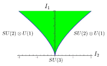
Figure 1: Manifold ${\cal M}$ of the $SU(3)$ invariants constructed from $x$=octet=hermitian, $3\times 3$, traceless matrix (green region). Each point of ${\cal M}$ represents the orbit of $x$, namely the set of points in octet space given by: $x_{g}=gxg^{-1}$, when $g$ runs over $SU(3)$. Boundaries of ${\cal M}$ are represented by Eq. (14). The little groups of the elements of different boundaries are indicated.

The boundaries of $\cal M$ are characterized by the rank of the Jacobian matrix being less than maximum Cabibbo:1970rza :

$$J=\frac{\partial(I_{1},I_{2},\cdots)}{\partial(x_{1},x_{2},\cdots)}~{},\qquad{\rm Rank}(J)=R<N~{}.$$ (15)

Boundaries are described by $R=N-1$ manifolds (e.g. surfaces, for $N=3$), each characterized by a different little group. Such manifolds meet along $R=N-2$ dimensional manifolds (e.g. lines) which in turn meet along even lower dimensionality manifolds (e.g. singular points), etc.. Each of these boundaries corresponds to a particular little group.

The extrema of $V(x)$ are to be found by solving the equations:

$$\frac{\partial V}{\partial x_{j}}=\sum_{i}\frac{\partial V}{\partial I_{i}}\frac{\partial I_{i}}{\partial x_{j}}=\sum_{i}\frac{\partial V}{\partial I_{i}}J_{ij}=0~{}.$$ (16)

We may now state the following.

• $V$ has always extrema on boundaries having as little group a maximal subgroup of ${\cal G}$ Michel:1970mua ;

• extrema of $V$ with respect to the points of a given boundary are extrema of $V(x)$ Cabibbo:1970rza .

The latter extrema are more natural than the generic extrema in the interior of $\cal M$, since they require the vanishing of only $N-1$, or $N-2$, etc. derivatives of $V$ given that, on the boundary, $J$ has 1 or 2, etc. vanishing eigenvectors (orthogonal to the boundary). Thus, from Fig. 1 we learn that it is more natural to break $SU(3)$ along the direction of the hypercharge Michel:1970mua ($x$ with two equal eigenvalues, little group $SU(2)\otimes U(1)$) than along the direction of $T_{3}$, which corresponds to elements in the interior of $\cal M$.

The case of chiral $SU(3)\otimes SU(3)$ was considered in Ref. Cabibbo:1970rza , with the symmetry broken by quark masses in the $(3,{\bar{3}})\oplus({\bar{3}},3)$. The elements of such representation are complex, $3\times 3$, matrices, $M$, transforming according to:

$$M\to M^{\prime}=UMV^{\dagger}~{}.$$

By one such transformation, one can reduce $M$ to the standard diagonal, positive, form ( up to an irrelevant overall phase Cabibbo:1970rza ):

$$M={\bar{U}}m{\bar{V}}^{\dagger}~{},\qquad m_{q}={\rm diag}(a,b,c)~{}.$$ (17)

There are three invariants, corresponding to the mass eigenvalues in Eq. (17):

$$I_{1}={\rm Tr}(MM^{\dagger})~{},\qquad I_{2}={\rm Tr}(MM^{\dagger}MM^{\dagger})~{},\qquad I_{3}={\rm Det}(M)~{},$$ (18)

and the natural extrema located on the boundaries correspond to the subgroups:

$$\begin{array}[]{lll}SU(2)\otimes U(1)&m_{q}={\rm diag}(a,a,c)&({\rm exact~{}isospin},~{}{\rm Rank=2})~{},\\ SU(2)\otimes SU(2)\otimes U(1)&m_{q}={\rm diag}(0,0,c)&({\rm hierarchical,~{}Rank}=1,~{}{\rm maximal})~{},\\ SU(3)&m_{q}={\rm diag}(a,a,a)&({\rm degenerate,~{}Rank}=1,~{}{\rm maximal})~{},\\ SU(3)\otimes SU(3)&m_{q}={\rm diag}(0,0,0)&({\rm symmetry~{}unbroken,~{}Rank}=0)~{}.\end{array}$$ (19)

Turning to our case, we note that there are no common matrices in the transformations of quarks, Eq. (9) or leptons, Eq. (10). This implies that the invariants divide in two independent sets: the Jacobian factorizes in two determinants and we can discuss the two cases separately.

4 Quarks in three families

To classify the invariants, we define two matrices which transform in the same way under $SU(3)_{q}$ and are singlet under the other transformations:

$$\rho_{U}=Y_{U}Y_{U}^{\dagger}~{},\qquad\rho_{D}=Y_{D}Y_{D}^{\dagger}~{};\qquad\rho_{U,D}\to U_{q}\rho_{U,D}U_{q}^{\dagger}~{}.$$ (20)

There are six unmixed invariants, which we may take as:

$$I_{U^{1}}={\rm Tr}(Y_{U}Y_{U}^{\dagger})~{},\quad I_{U^{2}}={\rm Tr}[(Y_{U}Y_{U}^{\dagger})^{2}]~{},\quad I_{U^{3}}={\rm Tr}[(Y_{U}Y_{U}^{\dagger})^{3}]~{},$$ (21)

and the same for $Y_{D}Y_{D}^{\dagger}$. Next we define four mixed invariants:

$$\begin{array}[]{ll}I_{U,D}={\rm Tr}(Y_{U}Y_{U}^{\dagger}Y_{D}Y_{D}^{\dagger})~{},&I_{U^{2},D}={\rm Tr}[(Y_{U}Y_{U}^{\dagger})^{2}Y_{D}Y_{D}^{\dagger})~{},\\ I_{U,D^{2}}={\rm Tr}[Y_{U}Y_{U}^{\dagger}(Y_{D}Y_{D}^{\dagger})^{2}]~{},&I_{(UD)^{2}}={\rm Tr}[(Y_{U}Y_{U}^{\dagger}Y_{D}Y_{D}^{\dagger})^{2}]~{}.\end{array}$$ (22)

As anticipated, 10 independent invariants suffice to characterize in generality the physical degrees of freedom in the Yukawa fields. We stress in particular that the 4 invariants in Eq. (22) contain enough information to reconstruct the 4 physical parameters of the CKM matrix, including its CP-violating phase (up to discreet choices, see Ref. Jenkins:2009dy ), despite none of them vanishes in the limit of exact CP invariance.

Unmixed invariants produce extrema corresponding to degenerate or hierarchical patterns as in the chiral case illustrated in (19). Mixed invariants involve the CKM matrix $U$, e.g.:

$$I_{U,D}={\rm Tr}(Y_{U}Y_{U}^{\dagger}Y_{D}Y_{D}^{\dagger})=\sum_{ij}U_{ij}U^{\star}_{ij}(m^{2}_{U})_{i}(m^{2}_{D})_{j}=\sum_{ij}P_{ij}(m^{2}_{U})_{i}(m^{2}_{D})_{j}~{}.$$ (23)

The matrix $P_{ij}=|U_{ij}|^{2}$ enjoys the properties that: all elements are between zero and 1, the sum of the elements of any row equals the sum of the elements of any column and both sums are equal to unity. Such matrices (by the so-called Birkhoff-Von Neumann theorem vonneumann ) are convex combinations of permutation matrices, i.e. matrices with a $1$ and all other null elements in each row, the $1$ being in different columns. Thus, permutation matrices provide us the singular points on the boundary of the domain, without having to compute the rank of the determinant. The upshot is that, after a relabeling of the $down$ quark coupled to each $up$ quark, we end up with $U_{\rm CKM}=1$.

A more detailed analysis is given in Ref. rodrigothesis . It involves the calculation of the $10\times 10$ Jacobian, which factorizes in two, $3\times 3$ Jacobians (unmixed invariants) and a $4\times 4$ one (mixed invariants) and it confirms the conclusion that one natural solution, for the three families quark case, is a hierarchical one, with dominating third family masses, and trivial CKM matrix.

In the limit of vanishing masses for the first two generations, this solution corresponds to the little group $SU(2)_{q}\otimes SU(2)_{U}\otimes SU(2)_{D}\otimes U(1)$ that is a maximal subgroup of $SU(3)_{q}\otimes SU(3)_{U}\otimes SU(3)_{D}$.

5 Leptons in three families

For leptons, we need 15 invariants. To construct them, we consider first the two combinations:

$$\rho_{E}=Y_{E}Y_{E}^{\dagger}~{},\qquad\rho_{\nu}=Y_{\nu}Y_{\nu}^{\dagger}~{};\qquad\rho_{E,\nu}\to U_{\ell}\rho_{E,\nu}U_{\ell}^{\dagger}~{},$$ (24)

in which ${\cal O}(3)$ transformations disappear. We may construct unmixed and mixed invariants, as in the quark case, the mixed ones involving the matrix $U_{L}$, Eq. (12). We choose the unmixed ones as:

$${\rm Unmixed,E:}\qquad I_{E^{1}}={\rm Tr}(Y_{E}Y_{E}^{\dagger})~{},\quad I_{E^{2}}={\rm Tr}[(Y_{E}Y_{E}^{\dagger})^{2}]~{},\quad I_{E^{3}}={\rm Tr}[(Y_{E}Y_{E}^{\dagger})^{3}]~{},$$ (25)

and three similar ones ($I_{\nu^{1-3}}$) using $\rho_{\nu}$, while the four mixed invariants containing $\rho_{e}$ and $\rho_{\nu}$ are taken to be:

$${\rm Mixed,~{}type~{}1}:\qquad\begin{array}[]{ll}I_{\nu,E}={\rm Tr}(Y_{\nu}Y_{\nu}^{\dagger}Y_{E}Y_{E}^{\dagger})~{},&I_{\nu^{2},E}={\rm Tr}[(Y_{\nu}Y_{\nu}^{\dagger})^{2}Y_{E}Y_{E}^{\dagger}]~{},\\ I_{\nu,E^{2}}={\rm Tr}[Y_{\nu}Y_{\nu}^{\dagger}(Y_{E}Y_{E}^{\dagger})^{2}]~{},&I_{(\nu E)^{2}}={\rm Tr}[(Y_{\nu}Y_{\nu}^{\dagger}Y_{E}Y_{E}^{\dagger})^{2}]~{}.\end{array}$$ (26)

For neutrinos we may construct also a matrix which transforms under the orthogonal group only:

$$\sigma_{\nu}=Y_{\nu}^{\dagger}Y_{\nu}~{};\qquad\sigma_{\nu}\to{\mathcal{O}}\sigma_{\nu}{\mathcal{O}}^{T}~{}.$$ (27)

The symmetric and antisymmetric parts of $\sigma_{\nu}$ transform separately and can be used to construct two different invariants, such as ${\rm Tr}[Y_{\nu}^{\dagger}Y_{\nu}(Y_{\nu}^{\dagger}Y_{\nu}\pm Y_{\nu}^{T}Y_{\nu}^{*})]$. Here the first term in the product gives back the invariant $I_{\nu^{2}}={\rm Tr}[(Y_{\nu}Y_{\nu}^{\dagger})^{2}]$, but the second one gives rise to new contractions which involve the unitary, symmetric matrix

$$W=U_{R}U_{R}^{T}~{}.$$ (28)

We thus define the following three additional invariants:

$${\rm Mixed,~{}type~{}2}:\qquad\begin{array}[]{ll}J_{\sigma^{1}}={\rm Tr}(Y_{\nu}^{\dagger}Y_{\nu}Y_{\nu}^{T}Y_{\nu}^{*})~{},&J_{\sigma^{2}}={\rm Tr}[(Y_{\nu}^{\dagger}Y_{\nu})^{2}Y_{\nu}^{T}Y_{\nu}^{*}]~{},\\ J_{\sigma^{3}}={\rm Tr}[(Y_{\nu}^{\dagger}Y_{\nu}Y_{\nu}^{T}Y_{\nu}^{*})^{2}]~{}.&\end{array}$$ (29)

Finally, we add two invariants which contain both $U_{L}$ and $W$:

$${\rm Mixed,~{}type~{}3}:\qquad\begin{array}[]{ll}I_{LR}=\mbox{Tr}\left[{\it Y}_{\nu}{\it Y}_{\nu}^{T}{\it Y}_{\nu}^{*}{\it Y}_{\nu}^{\dagger}{\it Y}_{E}{\it Y}_{E}^{\dagger}\right]~{},\\ I_{RL}=\mbox{Tr}\left[{\it Y}_{\nu}{\it Y}_{\nu}^{T}{\it Y}_{E}^{*}{\it Y}_{E}^{T}{\it Y}_{\nu}^{*}{\it Y}_{\nu}^{\dagger}{\it Y}_{E}{\it Y}_{E}^{\dagger}\right]~{}.\end{array}\qquad\qquad$$ (30)

The discussion of the Jacobian leads to the following results, see again Ref. rodrigothesis for details.

• Unmixed invariants produce extrema corresponding to degenerate or hierarchical mass patterns.

• Mixed, type 1, invariants contain $|(U_{L})_{ij}|^{2}$ and lead, like in the quark case, to the conclusion that $U_{L}$ is a permutation matrix (up to an overall phase).

• Mixed, type 2, invariants contain $|W_{ij}|^{2}$ and indicate that $W=U_{R}U_{R}^{T}$ is a also permutation matrix (up to an overall phase).

• Once we impose that $U_{L}$ and $W$ are permutation matrices, the sensitivity of Mixed, type 3 invariants to $\omega$ vanishes. The latter remains therefore undetermined.

We may absorb the first permutation matrix in a relabeling of the neutrinos coupled to each charged lepton, but the second matrix leads to a non trivial result for the neutrino mass matrix, Eq. (13). The reason for the difference is that, for quarks we could eliminate any complex matrix $U_{D}$ by a redefinition of $D_{R}$, but this is not possible for leptons, because we can redefine the $N_{i}$ only with a real orthogonal matrix.

We use the freedom in the neutrino labeling to set $U_{L}=1$ in the basis where charged leptons are ordered according to:

$${\it Y}_{E}=\mbox{diag}\,(y_{e},y_{\mu},y_{\tau})~{}.$$ (31)

There are four possible symmetric permutation matrices that can be associated with $W=U_{R}U_{R}^{T}$, one of them being the unit matrix. The other three imply non trivial mixing in one of the three possible neutrino pairs, e.g.

$$W=U_{R}U_{R}^{T}=-\left(\begin{array}[]{ccc}1&0&0\\ 0&0&1\\ 0&1&0\end{array}\right)$$ (32)

We introduced the minus sign for $W$ to have a positive determinant, consistently with the condition ${\rm Det}(U_{R})=1$.

Using this expression in Eq.(13) leads to

$$m_{\nu}=\frac{v^{2}}{M}~{}y_{\nu}\omega W\omega y_{\nu}=\frac{v^{2}}{M}~{}\left(\begin{array}[]{ccc}-y_{1}^{2}e^{2i\alpha}&0&0\\ 0&0&-y_{2}y_{3}e^{-i\alpha}\\ 0&-y_{2}y_{3}e^{-i\alpha}&0\end{array}\right)~{},$$ (33)

where $y_{\nu}=$ diag($y_{1},y_{2},y_{3}$) and $\omega$= diag($e^{i\alpha},e^{i\beta},e^{-i(\alpha+\beta}$). The absence of mixing between the first eigenvector of $m_{\nu}$ and those associated to the 2-3 sector implies that the phase $\alpha$ is unphysical and can be set to zero by an appropriate phase redefinition of the neutrino fields. From the second identity in Eq. (13) we then find:

$${\hat{m}}_{\nu}=\frac{v^{2}}{M}~{}{\rm diag}(y_{1}^{2},y_{2}y_{3},y_{2}y_{3})~{},$$

$$U_{\rm PMNS}^{(0)}=\left(\begin{array}[]{ccc}1&0&0\\ 0&1/\sqrt{2}&1/\sqrt{2}\\ 0&-1/\sqrt{2}&1/\sqrt{2}\end{array}\right)~{},\qquad\Omega={\rm diag}(-i,-i,1)~{}.$$ (37)

The non-trivial relative Majorana phase in the 2-3 sector is needed to bring all masses in positive form. The one maximal mixing angle and one maximal Majorana phase stem from the ${\mathcal{O}}(2)$ substructure in Eq. (33), as found in Ref. Alonso:2012fy ; Alonso:2013mca .

With three families we can go closer to the physical reality if we assume complete degeneracy for $y_{\nu}$. In this case, after the $2-3$ rotation we are left with degenerate $1$ and $2$ neutrinos and, a priori, a new rotation will be needed to align the neutrino basis with the basis in which the charged lepton mass takes the diagonal form in Eq. (31). We may expect, in this case, the PMNS matrix to have an additional rotation in the $1-2$ plane:

$$U_{\rm PMNS}=U_{\rm PMNS}^{(0)}~{}U(\theta_{12})~{}.$$ (38)

We shall see that small perturbations around the solution in Eq. (33) allow to determine this angle, that remains non-zero in the limit of vanishing perturbations.

6 Group theoretical considerations

One may ask what is the little group corresponding to the extremal solution, Eq. (33). While ${\it Y}_{\nu}$ transforms under $SU(3)_{\ell}\otimes{\cal O}(3)$, orthogonal transformations drop out of ${\it Y}_{\nu}{\it Y}_{\nu}^{T}$. In some sense we have to find the appropriate square root of $m_{\nu}$. By explicit calculation, one sees that the answer is given by:

$$Y_{\nu}={\left(\begin{array}[]{ccc}iy_{1}&0&0\\ 0&i\frac{y_{2}}{\sqrt{2}}&\frac{y_{2}}{\sqrt{2}}\\ 0&i\frac{y_{3}}{\sqrt{2}}&-\frac{y_{3}}{\sqrt{2}}\end{array}\right)~{}.}$$ (42)

${\it Y_{\nu}}$ transforms under $SU(3)_{\ell}\otimes{\cal O}(3)$ according to the $(\bar{3},3_{V})$ representation, where the suffix V denotes the vector representaton of $\mathcal{O}(3)$, realized, in triplet space, by the Gell-Mann imaginary matrices $\lambda_{2,5,7}$. One verifies that:

$$\lambda_{3}^{\prime}Y_{\nu}-Y_{\nu}\lambda_{7}=0;~{}\lambda_{3}^{\prime}={\rm diag}(0,1,-1)~{},$$ (43)

i.e. for this solution, $SU(3)_{\ell}\otimes{\cal O}(3)$ is reduced to the $U(1)_{\rm diag}$ subgroup of transformations of the form:

$$U(1)_{\rm diag}:~{}{\rm exp}\left(i\epsilon\lambda_{3}^{\prime}\right)\otimes{\rm exp}\left(i\epsilon\lambda_{7}\right)~{}.$$ (44)

This $U(1)_{\rm diag}$ is the little group of the boundary to which the solution in Eq. (42) belongs. When combined with a hierarchical solution for the charged-lepton Yukawa of the type $Y_{E}\propto(0,0,1)$, this corresponds to the little group $SU(2)_{E}\otimes U(1)_{\rm diag}$, a subgroup of $SU(3)_{E}\otimes SU(3)_{\ell}\otimes{\mathcal{O}(3)}$.

In the limit $y_{1}=y_{2}=y_{3}$, ${\it Y}_{\nu}$ becomes proportional to a unitary matrix:

$$Y_{\nu}\to y~{}{\left(\begin{array}[]{ccc}i&0&0\\ 0&i\frac{1}{\sqrt{2}}&\frac{1}{\sqrt{2}}\\ 0&i\frac{1}{\sqrt{2}}&-\frac{1}{\sqrt{2}}\end{array}\right)}=yV~{},\qquad VV^{\dagger}=1~{},$$ (48)

and the $U(1)$ invariance is augmented to a full ${\cal O}(3)_{\rm diag}$, a maximal subgroup of $SU(3)_{\ell}\otimes{\cal O}(3)$:

$$Y_{\nu}\to(V{\cal O}V^{\dagger})Y_{\nu}{\cal O}^{T}=Y_{\nu}~{},$$ (49)

where ${\cal O}$ is an orthogonal matrix generated by $\lambda_{2,5,7}$. The ${\cal O}(3)_{\rm diag}$ would remain unbroken only in the case of degenerate charged lepton masses. Combining $Y_{\nu}$ in Eq. (48) with $Y_{E}\propto(0,0,1)$, we recover the little group $SU(2)_{E}\otimes U(1)_{\rm diag}$.

Summarizing:

• $Y_{E}\propto(0,0,1):\quad SU(3)_{E}\otimes SU(3)_{\ell}\to SU(2)_{E}\otimes SU(2)_{\ell}\otimes U(1)\quad$ (maximal subgroup)

• $Y_{\nu}$ in (42) : $\qquad\quad{\hat{m}}_{\nu}={\rm diag}(m_{1},m,m)~{},\qquad~{}SU(3)_{\ell}\otimes{\cal O}(3)\to U(1)_{\rm diag}$

• $Y_{\nu}$ in (48) : $\quad\quad{\hat{m}}_{\nu}=m\times 1~{},\qquad~{}SU(3)_{\ell}\otimes{\cal O}(3)\to{\cal O}_{\rm diag}(3)$  (maximal subgroup)

• $Y_{E}\propto(0,0,1)$ & $Y_{\nu}$ in (42) or (48) : $\quad\ SU(3)_{E}\otimes SU(3)_{\ell}\otimes{\cal O}(3)\to SU(2)_{E}\otimes U(1)_{\rm diag}$

Both breaking patterns of $Y_{\nu}$ feature: i) at least two degenerate neutrinos; ii) $\theta_{23}=\frac{\pi}{4}$ and $\theta_{13}=0$; iii) one maximal Majorana phase. In addition, the degenerate pattern in Eq. (48) implies three degenerate neutrinos and a second large (not calculable) mixing angle.

We finally note that all the features of the degenerate pattern can also be obtained without assuming the existence of heavy right-handed neutrinos, but rather starting from the flavor symmetry group ${\cal G}_{0}$ in Eq. (1) and assuming that the effective (light) neutrino mass matrix,

$$\frac{1}{v^{2}}~{}{\bar{\ell}}_{L}m_{\nu}{\tilde{H}}{\tilde{H}}^{T}{\ell}^{C}_{L}~{},$$ (50)

breaks $SU(3)_{\ell}$ into the maximal subgroup $\mathcal{O}(3)_{\ell}$. This breaking pattern implies a neutrino mass matrix proportional to a unitary matrix. The latter must be a symmetric permutation matrix (in the basis where $Y_{E}$ is diagonal) in order to leave an unbroken $U(1)$ when combined with the charged-lepton Yukawa coupling. Selecting $U(1)_{\rm diag}$ among the possible unbroken subgroups we recover $m_{\nu}$ in Eq. (37) with $y_{1}^{2}=y_{2}y_{3}$.

7 Small perturbations

We now consider the addition of small perturbations to the matrix in Eq. (37), see for instance Refs. Altarelli:2004za , Blankenburg:2012nx . For simplicity, we analyze in detail the case of real perturbations. Under this assumption, the most general form of the perturbation is:

$$m_{\nu}={-}\frac{v^{2}y}{M}\left(\begin{array}[]{ccc}1+\delta+\sigma&\epsilon+\eta&\epsilon-\eta\\ \epsilon+\eta&\delta+\kappa&1\\ \epsilon-\eta&1&\delta-\kappa\end{array}\right)~{},$$ (51)

with $|\epsilon,\eta,\sigma,\delta,\kappa|\ll 1$. A simple calculation leads to the first order results:

$${\hat{m}}_{\nu}=m_{0}~{}{\rm diag}\left(1+\delta+\sqrt{2}\epsilon\frac{c}{s},1+\delta-\sqrt{2}\epsilon\frac{s}{c},1-\delta\right)~{},$$ (52)

$${\Omega={\rm diag}(-i,-i,1)}~{},$$ (53)

$$U_{\rm PMNS}=\left[\begin{array}[]{ccc}c&-s&\displaystyle\frac{\eta}{\sqrt{2}}\\ \displaystyle{\frac{s}{\sqrt{2}}}\left(1+\frac{c}{s}\frac{\eta}{\sqrt{2}}+\frac{\kappa}{2}\right)&\displaystyle{\frac{c}{\sqrt{2}}}\left(1-\frac{s}{c}\frac{\eta}{\sqrt{2}}+\frac{\kappa}{2}\right)&-\displaystyle\frac{1}{\sqrt{2}}\left(1-\frac{\kappa}{2}\right)\\ \displaystyle{\frac{s}{\sqrt{2}}}\left(1-\frac{c}{s}\frac{\eta}{\sqrt{2}}-\frac{\kappa}{2}\right)&\displaystyle{\frac{c}{\sqrt{2}}}\left(1+\frac{s}{c}\frac{\eta}{\sqrt{2}}-\frac{\kappa}{2}\right)&+\displaystyle\frac{1}{\sqrt{2}}\left(1+\frac{\kappa}{2}\right)\end{array}\right]~{},$$ (57)

where $s=\sin(\theta_{12})$, $c=\cos(\theta_{12})$, and $\tan(2\theta_{12})=2\sqrt{2}\epsilon/\sigma$.

The PMNS matrix features a generically large $\theta_{12}$ (that we cannot compute in absence of firm predictions for the values of $\epsilon$ and $\sigma$, but that does not goes to zero in the limit of vanishing perturbations), $\theta_{23}$ close to $\pi/4$, and $\theta_{13}$ generically small. With a suitable choice of the perturbations one can easily achieve the so-called bimaximal or tribimaximal mixing form.

The spectrum is almost degenerate, with normal or inverted hierarchy according to the signs of the perturbations, and mass splittings not correlated to the mixing matrix. Determining the size of the perturbations from $|\sin\theta_{13}|$ or, equivalently, from the deviation of $\theta_{23}$ from $\pi/4$, and assuming a similar size for the perturbation controlling the largest mass splitting, we find

$$\frac{|\Delta m^{2}_{\rm atm}|}{2m^{2}_{0}}\approx|\sin\theta_{13}|\approx|\theta_{12}-\frac{\pi}{4}|\approx 0.1\quad\longrightarrow\quad m_{0}\approx 0.1~{}{\rm eV}~{}.$$ (58)

A lightest neutrino mass of this size is within reach of the next generation of $0\nu\nu$ double beta decay experiments pdg , and possibly of cosmological measurements Ade:2013zuv ; Ade:2013lmv . Note also that the size of the perturbations is not far from what could be deduced from the charged lepton spectrum, treating $m_{\mu}/m_{\tau}\approx 0.06$ as estimate of the sub-leading terms.

So far we considered only real perturbations. Assuming complex perturbations does not change qualitatively the results listed above for the mass spectrum and the mixing angles, but leads to non-vanishing CP-violating phases. In particular, we find a generically large Dirac-type phase and a generically large second Majorana phase (that becomes physical), while small corrections to the maximal Majorana phase in the 2-3 sector. In this context, we note that small Majorana phases are enough for successful leptogenesis with almost degenerate right-handed neutrinos masses (see e.g. Ref. O3Rleptogenesis ).

In this letter we shall not try to identify the origin of the small perturbations. Given the non-perturbative character of the argument that leads to the $U(1)_{\rm diag}$ symmetric boundary, the latter symmetry cannot obviously be lifted by ${\cal G}$ symmetric interactions in higher perturbative order. Small perturbations may result however from the effect of other fields, transforming differently from the $Y$’s and acquiring smaller vevs, like e.g. in Refs. Barbieri:1995uv ; Alonso:2011yg ; Blankenburg:2012nx , or by the effect of interactions external to the present scheme, e.g. arising from gravity.

8 Conclusions and outlook

We have assumed that the structure of quark and lepton mass matrices derives from a minimum principle, with the maximal flavor symmetry $\left[SU(3)\right]^{5}\otimes{\mathcal{O}}(3)$ and a minimal breaking due to the vevs of fields transforming like the Yukawa couplings. For leptons we find a natural solution correlating large mixing angles and degenerate neutrinos. This solution generalizes to three familes and arbitrary invariant potential the results found in Ref. Alonso:2012fy ; Alonso:2013mca . The generalization of this result to arbitrary see-saw models has also been discussed. Subject to small perturbations, the solution can reproduce the observed pattern of neutrino masses and mixing angles. Our considerations lead to a value of the common neutrino mass that is within reach of the next generation of neutrinoless double beta decay experiments, and possibly within that of cosmological measurements.

References

- (1) R. S. Chivukula and H. Georgi, Phys. Lett. B188 (1987) 99.
- (2) P. Minkowski, Phys. Lett. B 67 (1977) 421; M. Gell-Mann, P. Ramond and R. Slansky, Conf. Proc. C 790927 (1979) 315; R. N. Mohapatra and G. Senjanovic, Phys. Rev. Lett. 44 (1980) 912;
- (3) V. Cirigliano, B. Grinstein, G. Isidori, and M. B. Wise, Nucl. Phys. B728 (2005) 121 [ hep-ph/0507001].
- (4) F. Englert and R. Brout, Phys. Rev. Lett. 13 (1964) 321; P. W. Higgs, Phys. Lett. 12 (1964) 132. and Phys. Rev. Lett. 13 (1964) 508; G. S. Guralnik, C. R. Hagen and T. W. B. Kibble, Phys. Rev. Lett. 13 (1964) 585.
- (5) G. Isidori, Y. Nir, and G. Perez, Ann. Rev. Nucl. Part. Sci. 60 (2010) 355 [arXiv:1002.0900].
- (6) G. D’Ambrosio, G. F. Giudice, G. Isidori, and A. Strumia Nucl. Phys. B645 (2002) 155 [hep-ph/0207036].
- (7) S. Davidson and F. Palorini, Phys. Lett. B642 (2006) 72 [hep-ph/0607329].
- (8) M. B. Gavela, T. Hambye, D. Hernandez and P. Hernandez, JHEP 0909 (2009) 038 [arXiv:0906.1461].
- (9) A. S. Joshipura, K. M. Patel and S. K. Vempati, Phys. Lett. B 690 (2010) 289 [arXiv:0911.5618 [hep-ph]].
- (10) R. Alonso, G. Isidori, L. Merlo, L. A. Munoz, and E. Nardi, JHEP 06 (2011) 037 [ arXiv:1103.5461].
- (11) B. Grinstein, M. Redi, and G. Villadoro, JHEP 1011 (2010) 067 [arXiv:1009.2049].
- (12) L. Michel and L. A. Radicati, Proc. of the Fifth Coral Gables Conference on Symmetry principles at High Energy, ed. by B. Kursunoglu et al., W. H. Benjamin, Inc. New York (1965); Annals Phys. 66 (1971) 758.
- (13) N. Cabibbo and L. Maiani, in Evolution of particle physics, Academic Press (1970), 50, App. I.
- (14) E. E. Jenkins and A. V. Manohar, JHEP 0910 (2009) 094 [arXiv:0907.4763 [hep-ph]] and references within; A. Hanany, E. E. Jenkins, A. V. Manohar and G. Torri, JHEP 1103 (2011) 096 [arXiv:1010.3161 [hep-ph]]
- (15) C. D. Froggatt, H. B. Nielsen, Nucl. Phys. B147 (1979) 277.
- (16) A. Anselm and Z. Berezhiani, Nucl.Phys. B484 (1997) 97 [hep-ph/9605400].
- (17) R. Barbieri, L. J. Hall, G. L. Kane and G. G. Ross, [hep-ph/9901228].
- (18) Z. Berezhiani and A. Rossi, Nucl.Phys.Proc.Suppl. 101 (2001) 410 [hep-ph/0107054].
- (19) P. F. Harrison and W. G. Scott, Phys. Lett. B 628 (2005) 93 [hep-ph/0508012].
- (20) T. Feldmann, M. Jung and T. Mannel, Phys. Rev. D 80 (2009) 033003 [arXiv:0906.1523 [hep-ph]].
- (21) R. Alonso, M. Gavela, L. Merlo, and S. Rigolin, JHEP 1107 (2011) 012 [arXiv:1103.2915].
- (22) E. Nardi, Phys. Rev. D 84 (2011) 036008 [arXiv:1105.1770].
- (23) J. R. Espinosa, C. S. Fong and E. Nardi, JHEP 1302 (2013) 137 [arXiv:1211.6428]
- (24) R. Alonso, M. Gavela, D. Hernandez, and L. Merlo, Phys.Lett. B715 (2012), 194 [arXiv:1206.3167].
- (25) R. Alonso, M. B. Gavela, D. Hernandez, L. Merlo and S. Rigolin, JHEP 1308 (2013) 069 [arXiv:1306.5922 [hep-ph]].
- (26) P. F. Harrison, D. H. Perkins and W. G. Scott, Phys. Lett. B 530 (2002) 167 [hep-ph/0202074] G. Altarelli and F. Feruglio, Nucl. Phys. B 720 (2005) 64 [hep-ph/0504165]; and Nucl. Phys. B 741 (2006) 215 [hep-ph/0512103]; F. Bazzocchi, L. Merlo and S. Morisi, Nucl. Phys. B 816 (2009) 204 [arXiv:0901.2086].
- (27) J. Beringer et al. (Particle Data Group), Phys. Rev. D86, 010001 (2012)
- (28) P. A. R. Ade et al. [Planck Collaboration], “Planck 2013 results. XVI. Cosmological parameters,” arXiv:1303.5076 [astro-ph.CO].
- (29) P. A. R. Ade et al. [Planck Collaboration], arXiv:1303.5080 [astro-ph.CO].
- (30) G. Blankenburg, G. Isidori and J. Jones-Perez, Eur. Phys. J. C 72 (2012) 2126 [arXiv:1204.0688]
- (31) A. Broncano, M. B. Gavela and E. E. Jenkins, Phys. Lett. B 552 (2003) 177 [Erratum-ibid. B 636 (2006) 330] [hep-ph/0210271]; E. E. Jenkins and A. V. Manohar, Nucl. Phys. B 792 (2008) 187 [arXiv:0706.4313].
- (32) J. A. Casas and A. Ibarra, Nucl. Phys. B 618 (2001) 171 [hep-ph/0103065].
- (33) See e.g. R. B. Bapat, Indian Statistical Institute, New Delhi and T. E. S. Raghavan, Nonnegative Matrices and Applications, Encyclopedia of Mathematics and its Applications 64, Cambridge University Press, Cambridge (1997).
- (34) R. Alonso, Ph.D. Thesis arXiv:1307.1904 [hep-ph].
- (35) G. Altarelli and F. Feruglio, New J. Phys. 6 (2004) 106 [hep-ph/0405048]; L. J. Hall and G. G. Ross, arXiv:1303.6962 [hep-ph].
- (36) V. Cirigliano, G. Isidori and V. Porretti, Nucl. Phys. B 763 (2007) 228 [hep-ph/0607068]; G. C. Branco et al., JHEP 0709 (2007) 004 [hep-ph/0609067]; V. Cirigliano et al. JCAP 0801 (2008) 004 [arXiv:0711.0778].
- (37) R. Barbieri, G. R. Dvali and L. J. Hall, Phys. Lett. B 377 (1996) 76 [hep-ph/9512388].