A Robust Multilevel Method for Hybridizable Discontinuous Galerkin Method for the Helmholtz Equation

Abstract

A robust multilevel preconditioner based on the hybridizable discontinuous Galerkin method for the Helmholtz equation with high wave number is presented in this paper. There are two keys in our algorithm, one is how to choose a suitable intergrid transfer operator, and the other is using GMRES smoothing on coarse grids. The multilevel method is performed as a preconditioner in the outer GMRES iteration. To give a quantitative insight of our algorithm, we use local Fourier analysis to analyze the convergence property of the proposed multilevel method. Numerical results show that for fixed wave number, the convergence of the algorithm is mesh independent. Moreover, the performance of the algorithm depends relatively mildly on wave number.

Key words. Multilevel method, Helmholtz equation, high wave number, hybridizable discontinuous Galerkin method, GMRES method, local Fourier analysis

1 Introduction

In this paper we consider the Helmholtz equation with Robin boundary condition which is the first order approximation of the radiation condition. The equation is written in a mixed form as follows: Find $({{\boldsymbol{q}}},u)$ such that

$${\bf i}\kappa{{\boldsymbol{q}}}+\nabla u =0\qquad{\rm in}\ \Omega,$$ (1.1)

$${\bf i}\kappa u+{\rm div}\,{{\boldsymbol{q}}} =f\qquad{\rm in}\ \Omega,$$ (1.2)

$$-{{\boldsymbol{q}}}\cdot{{\boldsymbol{n}}}+u =g\qquad{\rm on}\ \partial\Omega,$$ (1.3)

where $\Omega\subset\mathbb{R}^{d}$, $d=2,3$, is a polygonal or polyhedral domain, $\kappa>0$ is known as the wave number, ${\bf i}=\sqrt{-1}$ denotes the imaginary unit, and ${{\boldsymbol{n}}}$ denotes the unit outward normal to $\partial\Omega$. Helmholtz equation finds applications in many important fields, e.g., in acoustics, seismic inversion and electromagnetic, but how to solve the Helmholtz equation efficiently is still of great challenge.

The strong indefiniteness has prevented the standard multigrid methods from being directly applied to the discrete Helmholtz equation. In [9], Elman, Ernst and O’Leary modified the standard multigrid algorithm by adding GMRES iterations as corrections on coarse grids and using it as an outer iteration. But in order to obtain a satisfactory convergence behavior, a relatively large number of GMRES smoothing should be performed on coarse grids which leads to relatively large memory requirement, so the optimality of the multigrid algorithm cannot be guaranteed. In [6], the authors utilized the continuous interior penalty finite element methods [23, 24] to construct the stable coarse grid correction problems, which reduces the steps of GMRES smoothing on coarse grids. Based on the fact that the error components which cannot be reduced by the standard multigrid can be factorized by representing it as the product of a certain high-frequency Fourier component and a ray function, Brandt and Livshits introduced so-called wave-ray multigrid methods in [3, 20]. Although this method exhibits high convergence rate with increasing wave number, it does not easily generalize to unstructured grids and complicated Helmholtz problems. Besides, shifted Laplacian preconditioners [13, 14] and sweeping preconditioners [10, 11] based on an approximate $LDL^{t}$ factorization were introduced to solve the Helmholtz equation with high wave number. A survey of the development of fast iterative solvers can be found in [12, 15].

Hybridizable discontinuous Galerkin (HDG) method has two main advantages in the discretization of Helmholtz equation. First, it is a stable method, which means that the discrete system is always well-posed without any mesh constraint. Rigorous convergence analysis of the HDG method for Helmholtz equation can be found in [5]. Second, comparing to standard discontinuous Galerkin method, HDG method results in significantly reducing the degrees of freedom, especially when the polynomial degree $p$ is large. However, to the best of our knowledge, no efficient iterative method or preconditioner for HDG discretization system for the Hemholtz equation in the literature has been proposed.

The hybridized system is a linear equation for Lagrange multipliers which is obtained by eliminating the flux as well as the primal variable. For the second-order elliptic problems, a Schwarz preconditioner for the algebraic system was presented in [18]. In [19], the authors consider the application of a variable V-cycle multigrid algorithm for the hybridized mixed method for second-order elliptic boundary value problems. In their multigrid algorithm, both smoothing and correction on coarse grids are based on standard piecewise linear continuous finite element discretization system. The convergence of the multigrid algorithm is dependent on an assumption that the number of smoothings increases in a specific way (see Theorem 3.1 in [19] for details). The critical ingredient in the algorithm is how to choose a suitable intergrid transfer operator. Numerical experiments in [19] show that certain ‘obvious’ transfer operators lead to slow convergence.

The objective of this paper is to propose a robust multilevel method for the HDG method approximation of the Helmholtz equation. The main ingredients in multilevel method are how to construct coarse grid correction problem and perform efficient smoothing. Since strong indefiniteness arises for Helmholtz equation with large wave number, standard Jacobi or Gauss-Seidel smoothers become unstable on the coarse grids. Motivated by the idea in [9], we use GMRES smoothing for those coarse grids. Unlike the smoothing strategy in [9], the number of GMRES smoothing steps in our algorithm is much smaller, even if one smoothing step may guarantee the convergence of our multilevel algorithm. Moreover, both smoothing on fine and coarse grids in our multilevel method are based on hybridized system of Lagrange multiplier on each level.

Local Fourier analysis (LFA) has been introduced for multigrid analysis by Achi Brandt in 1977 (cf. [2]). We mainly utilize the LFA to analyze smoothing properties of relaxations and convergence properties of two and three level methods in the one dimensional case. This may provide quantitative insights into the proposed multilevel method for Helmholtz problem (1.1)-(1.3). A survey for LFA can be found in [22].

The remainder of this paper is organized as follows: In section 2, we firstly review the formulation of HDG method for the Helmholtz equation and present our multilevel algorithm. The stability estimate of the intergrid transfer operator will be carried out in section 3. Section 4 is devoted to the LFA of the multilevel method in one dimensional case. Finally, we give some numerical results to demonstrate the performance of our multilevel method.

2 HDG method and its multilevel algorithm

Let $\mathcal{T}_{h}$ be a quasi-uniform subdivision of $\Omega$, and denote the collection of edges (faces) by $\mathcal{E}_{h}$, while the set of interior edges (faces) by $\mathcal{E}_{h}^{0}$ and the collection of element boundaries by $\partial\mathcal{T}_{h}:=\{\partial T|T\in\mathcal{T}_{h}\}$. We define $h_{T}:={\rm diam}(T)$ and let $h:={\rm max}_{T\in{\mathcal{T}}_{h}}h_{T}$. Throughout this paper we use the standard notations and definitions for Sobolev spaces (see, e.g., Adams[1]).

On each element $T$ and each edge (face) $F$, we define the local spaces of polynomials of degree $p\geq 1$:

$${{\boldsymbol{V}}}(T):=(\mathcal{P}_{p}(T))^{d},\qquad W(T):=\mathcal{P}_{p}(T),\qquad M(F):=\mathcal{P}_{p}(F),$$

where $\mathcal{P}_{p}(S),S=T$ or $F$, denotes the space of polynomials of total degree at most $p$ on $S$. The corresponding global finite element spaces are given by

$${{\boldsymbol{V}}}_{h}^{p}: =\{{{\boldsymbol{v}}}\in{{\boldsymbol{L}}}^{2}(\Omega)\ |\ {{\boldsymbol{v}}}|_{T}\in{{\boldsymbol{V}}}(T)\ {\rm for\ all}\ T\in\mathcal{T}_{h}\},$$

$$W_{h}^{p}: =\{w\in L^{2}(\Omega)\ |\ w|_{T}\in W(T)\ {\rm for\ all}\ T\in\mathcal{T}_{h}\},$$

$$M_{h}^{p}: =\{\mu\in L^{2}(\mathcal{E}_{h})\ |\ \mu|_{F}\in M(F)\ {\rm for\ all}\ F\in\mathcal{E}_{h}\},$$

where ${{\boldsymbol{L}}}^{2}(\Omega):=(L^{2}(\Omega))^{d}$, $L^{2}(\mathcal{E}_{h}):=\Pi_{F\in\mathcal{E}_{h}}L^{2}(F)$. On these spaces we define the bilinear forms

$$({{\boldsymbol{v}}},{{\boldsymbol{w}}})_{\mathcal{T}_{h}}:=\sum_{T\in\mathcal{T}_{h}}({{\boldsymbol{v}}},{{\boldsymbol{w}}})_{T},\ (v,w)_{\mathcal{T}_{h}}:=\sum_{T\in\mathcal{T}_{h}}(v,w)_{T},\ {\rm and}\ \langle v,w\rangle_{\partial\mathcal{T}_{h}}:=\sum_{T\in\mathcal{T}_{h}}\langle v,w\rangle_{\partial T},$$

with $({{\boldsymbol{v}}},{{\boldsymbol{w}}})_{T}:=\int_{T}{{\boldsymbol{v}}}\cdot{{\boldsymbol{w}}}dx$, $(v,w)_{T}:=\int_{T}{v}{w}dx$ and $\langle v,w\rangle_{\partial T}:=\int_{\partial T}{v}{w}ds$.

The HDG method yields finite element approximations $({{\boldsymbol{q}}}_{h},u_{h},\hat{u}_{h})\in{{\boldsymbol{V}}}_{h}^{p}\times W_{h}^{p}\times M_{h}^{p}$ which satisfy

$$({\bf i}\kappa{{\boldsymbol{q}}}_{h},\overline{{\boldsymbol{r}}})_{\mathcal{T}_{h}}-(u_{h},\overline{{\rm div\,{{\boldsymbol{r}}}}})_{\mathcal{T}_{h}}+\langle\hat{u}_{h},\overline{{{\boldsymbol{r}}}\cdot{{\boldsymbol{n}}}}\rangle_{\partial\mathcal{T}_{h}} =0,$$ (2.1)

$$({\bf i}\kappa u_{h},\overline{w})_{\mathcal{T}_{h}}-({{\boldsymbol{q}}}_{h},\overline{\nabla w})_{\mathcal{T}_{h}}+\langle\hat{{\boldsymbol{q}}}_{h}\cdot{{\boldsymbol{n}}},\overline{w}\rangle_{\partial\mathcal{T}_{h}} =(f,\overline{w})_{\mathcal{T}_{h}},$$ (2.2)

$$\langle-\hat{{\boldsymbol{q}}}_{h}\cdot{{\boldsymbol{n}}}+\hat{u}_{h},\overline{\mu}\rangle_{\partial\Omega} =\langle g,\overline{\mu}\rangle_{\partial\Omega},$$ (2.3)

$$\langle\hat{{\boldsymbol{q}}}_{h}\cdot{{\boldsymbol{n}}},\overline{\mu}\rangle_{\partial\mathcal{T}_{h}\backslash\partial\Omega} =0,$$ (2.4)

for all ${{\boldsymbol{r}}}\in{{\boldsymbol{V}}}_{h}^{p}$, $w\in W_{h}^{p}$, and $\mu\in M_{h}^{p}$, where the overbar denotes complex conjugation. The numerical flux $\hat{{\boldsymbol{q}}}_{h}$ is given by

$$\hat{{\boldsymbol{q}}}_{h}={{\boldsymbol{q}}}_{h}+\tau_{h}(u_{h}-\hat{u}_{h}){{\boldsymbol{n}}}\qquad{\rm on}\ \partial\mathcal{T}_{h},$$ (2.5)

where the parameter $\tau_{h}$ is the so-called local stabilization parameter which has an important effect on both the stability of the solution and the accuracy of the HDG scheme. Let $\tau_{h,T}$ be the value of $\tau_{h}$ on the element $T$. We always choose $\tau_{h,T}=\frac{p}{\kappa h_{T}}$. One of the advantages of HDG methods is the elimination of both ${{\boldsymbol{q}}}_{h}$ and $u_{h}$ from the equation, and then we may obtain a formulation in terms of $\hat{u}_{h}$ only. Next we define the discrete solutions of the local problems: For each function $\lambda\in M_{h}^{p}$, $({\bf\mathcal{Q}}_{\lambda},\mathcal{U}_{\lambda})\in{{\boldsymbol{V}}}(T)\times W(T)$ satisfies the following formulation

$$({\bf i}\kappa\mathcal{Q}_{\lambda},\overline{{{\boldsymbol{r}}}})_{T}-(\mathcal{U}_{\lambda},\overline{{\rm div}\,{{\boldsymbol{r}}}})_{T} =-\langle\lambda,\overline{{{\boldsymbol{r}}}\cdot{{\boldsymbol{n}}}}\rangle_{\partial T},\quad\forall{{\boldsymbol{r}}}\in{{\boldsymbol{V}}}(T),$$ (2.6)

$$({\bf i}\kappa\mathcal{U}_{\lambda},\overline{w})_{T}-(\mathcal{Q}_{\lambda},\overline{\nabla w})_{T}+\langle\hat{\mathcal{Q}}_{\lambda}\cdot{{\boldsymbol{n}}},\overline{w}\rangle_{\partial T} =0,\quad\forall{w}\in W(T),$$ (2.7)

where $\hat{\mathcal{Q}}_{\lambda}\cdot{{\boldsymbol{n}}}=\mathcal{Q}_{\lambda}\cdot{{\boldsymbol{n}}}+\tau_{h}(\mathcal{U}_{\lambda}-\lambda)$. For $f\in L^{2}(\Omega)$, $({\bf\mathcal{Q}}_{f},\mathcal{U}_{f})\in{{\boldsymbol{V}}}(T)\times W(T)$ is defined as follows:

$$({\bf i}\kappa\mathcal{Q}_{f},\overline{{{\boldsymbol{r}}}})_{T}-(\mathcal{U}_{f},\overline{{\rm div}\,{{\boldsymbol{r}}}})_{T} =0,\quad\forall{{\boldsymbol{r}}}\in{{\boldsymbol{V}}}(T),$$ (2.8)

$$({\bf i}\kappa\mathcal{U}_{f},\overline{w})_{T}-(\mathcal{Q}_{f},\overline{\nabla w})_{T}+\langle\hat{\mathcal{Q}}_{f}\cdot{{\boldsymbol{n}}},\overline{w}\rangle_{\partial T} =(f,\overline{w})_{T},\quad\forall{w}\in W(T),$$ (2.9)

where $\hat{\mathcal{Q}}_{f}\cdot{{\boldsymbol{n}}}=\mathcal{Q}_{f}\cdot{{\boldsymbol{n}}}+\tau_{h}\mathcal{U}_{f}$. Then $\hat{u}_{h}$ is the solution of the following equation

$$a_{h}(\hat{u}_{h},\mu)=b_{h}(\mu),\quad\forall\mu\in M_{h}^{p},$$ (2.10)

where

$$a_{h}(\lambda,\mu):=-\langle\hat{\mathcal{Q}}_{\lambda},\overline{\mu}\rangle_{\partial\mathcal{T}_{h}}+\langle\lambda,\overline{\mu}\rangle_{\partial\Omega},$$ (2.11)

$$b_{h}(\mu):=\langle\hat{\mathcal{Q}}_{f},\overline{\mu}\rangle_{\partial\mathcal{T}_{h}}+\langle g,\overline{\mu}\rangle_{\partial\Omega}.$$

We focus on designing a multilevel method for the linear algebraic system (2.10).

Let $\{\mathcal{T}_{l}\}_{l=0}^{L}$ be a shape regular family of nested conforming triangulations of $\Omega$, which means that $\mathcal{T}_{0}$ is a quasi-uniform initial mesh and $\mathcal{T}_{l}$ is obtained by quasi-uniform refinement of $\mathcal{T}_{l-1},l\geq 1$. For simplicity, we denote by $a_{l}(\cdot,\cdot)$ the bilinear form $a_{h_{l}}(\cdot,\cdot)$ on $M_{l}$, where $h_{l}$ is the mesh size of ${\mathcal{T}}_{l}$, meanwhile we denote by $M_{l}$ for the $hp$-HDG approximation space $M^{p}_{h_{l}}$ on ${\mathcal{T}}_{l}$, the collection of edges of ${\mathcal{T}}_{l}$ is denoted by $\mathcal{E}_{l}$. Let $I_{l}:M_{l}\rightarrow M_{L}$ be the intergrid transform operator, which will be specified later. Define projections $P_{l}$, $Q_{l}$ : $M_{L}\rightarrow M_{l}$ as

$$a_{l}(P_{l}v,w)=a_{L}(v,I_{l}w),\quad\langle Q_{l}v,\overline{w}\rangle_{\partial{\mathcal{T}}_{l}}=\langle v,\overline{I_{l}w}\rangle_{\partial{\mathcal{T}}_{L}},\quad v\in M_{L},\,w\in M_{l}.$$

The existence and uniqueness solution of problem (2.10) imply the well-posedness of the above definition. For $0\leq l\leq L$, define $A_{l}:M_{l}\rightarrow M_{l}$, $F_{l}\in M_{l}$ by means of

$$\langle A_{l}v,\overline{w}\rangle_{\partial{\mathcal{T}}_{l}}=a_{l}(v,w),\ \langle F_{l},\overline{w}\rangle_{\partial{\mathcal{T}}_{l}}=b_{l}(w),\quad v,w\in M_{l}.$$ (2.12)

Let $R_{l}:M_{l}\rightarrow M_{l}$ be the smoothing operator on $M_{l}$ which is chosen as weighted Jacobi or Gauss-Seidel relaxation. In fact, both weighted Jacobi and Gauss-Seidel relaxation can be used on the fine grids. Otherwise, we choose GMRES relaxation as a smoother, and we will give some illustration in Section 4. Now we state our multilevel method.

Algorithm 2.1.

Given an arbitrarily chosen initial iterate $u^{0}\in M_{L}$, we seek $u^{n}\in M_{L}$ as follows:

Let $v_{0}=u^{n-1}$. For $l=0,1,\cdots,L$, compute $v_{l+1}$ by

$1)$ When $l=0$, $v_{1}=v_{0}+\mu_{0}I_{0}(A_{0})^{-1}Q_{0}(F_{L}-A_{L}v_{0})$. For $l=1,\cdots,L$, if $\kappa h_{l}/p\geq\alpha$, perform $m_{1}$ steps GMRES smoothing for the correction problem $A_{l}w_{l}=Q_{l}(F_{L}-A_{L}v_{l})$, and set

$$v_{l+1}=v_{l}+\mu_{l}I_{l}w_{l},$$

else perform $m_{2}$ steps of weighted Jacobi relaxation $R^{J}_{l}$ or Gauss-Seidel relaxation $R^{GS}_{l}$,

$$v_{l+1}=v_{l}+\mu_{l}I_{l}(R_{l})^{m_{2}}Q_{l}(F_{L}-A_{L}v_{l}),$$

where $R_{l}=R^{J}_{l}$ or $R^{GS}_{l}$. We will always choose the parameters $\alpha$ and $\{\mu_{l}\}^{L}_{l=0}$ as $0.5$ in this paper.

$2)$ For $l=L,\cdots,1$, if $\kappa h_{l}/p<\alpha$, perform $m_{3}$ steps of $R_{l}=R^{J}_{l}$ or $R^{GS}_{l}$ to obtain $v_{2L+2-l}$,

$$v_{2L+2-l}=v_{2L+1-l}+\mu_{l}I_{l}(R_{l})^{m_{3}}Q_{l}(F_{L}-A_{L}v_{2L+1-l});$$

else perform $m_{4}$ steps of GMRES smoothing for the correction problem $A_{l}w_{l}=Q_{l}(F_{L}-A_{L}v_{2L+1-l})$, and set

$$v_{2L+2-l}=v_{2L+1-l}+\mu_{l}I_{l}w_{l}.$$

When $l=0$, $v_{2L+2}=v_{2L+1}+\mu_{0}I_{0}(A_{0})^{-1}Q_{0}(F_{L}-A_{L}v_{2L+1})$.

$3)$ Set $u^{n}=v_{2L+2}$.

At the end of this section, we give the definition of the transfer operator $I_{l}:M_{l}\rightarrow M_{L},0\leq l\leq L-1$. Note that $I_{L}:M_{L}\rightarrow M_{L}$ is the identity operator. Denote $W_{l}^{c}:=\{v\in C(\Omega)\ |\ v|_{T}\in W(T),\ \forall T\in\mathcal{T}_{l}\}$. We first define an auxiliary operator $I_{l}^{W}:M_{l}\rightarrow W_{l}^{c},0\leq l\leq L-1$.

Case 1: $p=1$. Let

$$I_{l}^{W}\lambda(z_{n})=\frac{\sum_{e\subset\mathcal{E}_{l}(z_{n})}\lambda_{e}(z_{n})}{|\mathcal{E}_{l}(z_{n})|}\quad\forall z_{n}\in\mathcal{V}_{l},$$

where $\mathcal{V}_{l}$ is the collection of the vertices of ${\mathcal{T}}_{l}$. For any $z_{n}\in\mathcal{V}_{l}$, $\mathcal{E}_{l}(z_{n})$ is the collection of edges in $\mathcal{E}_{l}$ which contain $z_{n}$, while $|\mathcal{E}_{l}(z_{n})|$ is the number of edges in $\mathcal{E}_{l}(z_{n})$.

Case 2: $p=2$. Let

$$I_{l}^{W}\lambda(z_{n})=\left\{\begin{array}[]{ll}\frac{\sum_{e\subset\mathcal{E}_{l}(z_{n})}\lambda_{e}(z_{n})}{|\mathcal{E}_{l}(z_{n})|}&z_{n}\in\mathcal{V}_{l};\\ \lambda(z_{n})&z_{n}\in\mathcal{N}_{l}\backslash\mathcal{V}_{l},\end{array}\right.\\$$

where $\mathcal{N}_{l}$ is the degree of freedom of the space $W_{l}^{c}$.

Case 3: $p\geq 3$. Let

$$I_{l}^{W}\lambda(z_{n})=\left\{\begin{array}[]{ll}\frac{\sum_{e\subset\mathcal{E}_{l}(z_{n})}\lambda_{e}(z_{n})}{|\mathcal{E}_{l}(z_{n})|}&z_{n}\in\mathcal{V}_{l};\\ \lambda(z_{n})&z_{n}\in\mathcal{N}_{l}\backslash(\mathcal{V}_{l}\cup\mathcal{N}_{l}^{0});\\ U_{\lambda}(z_{n})&z_{n}\in\mathcal{N}_{l}^{0},\end{array}\right.\\$$

where $\mathcal{N}_{l}^{0}$ is the degree of freedom in the interior of every element $T\in{\mathcal{T}}_{l}$. For the $p\geq 3$ case, $\mathcal{N}_{l}^{0}$ is not an empty set, but the space $M_{l}$ dose not provide any information for the degree of freedom in the interior of $T$. Hence we use the solution of the local problem (2.6-2.7) to define it. Note that this procedure only involves the computation of the local problems and can be parallel implemented.

With the help of the above operator $I_{l}^{W}$, we may define $I_{l}:M_{l}\rightarrow M_{L},0\leq l\leq L-1$ as follows:

$$I_{l}\mu|_{\mathcal{E}_{L}}:=I_{l}^{W}\mu|_{\mathcal{E}_{L}}.$$ (2.13)

Throughout this paper, we use notations $A\lesssim B$ and $A\gtrsim B$ for the inequalities $A\leq CB$ and $A\geq CB$, where $C$ is a positive number independent of the mesh sizes and mesh levels.

3 The stability of the intergrid transfer operator

The design of the stable intergrid transfer operator is critical for the success of the nonnested multilevel method. The failure of certain ‘obvious’ transfer operators in [19] is due to the fact that the energy error increases by using these operators. In the following, we will analyze the stability estimate of our intergrid transfer operator in the energy norm. From the numerical results, we may find that this intergrid transfer operator works well in our multilevel method for the Helmholtz problem. Consider the Possion equation:

$$-\triangle U=f\qquad{\rm{in}}\ \Omega,$$ (3.1)

$$U=g\qquad{\rm{on}}\ \partial\Omega,$$ (3.2)

where $f\in L^{2}(\Omega)$ and $g\in L^{2}(\partial\Omega)$. Clearly, (3.1-3.2) can be rewritten in a mixed form as finding $({{\boldsymbol{Q}}},U)$ such that

$${\boldsymbol{Q}}=-\nabla U\qquad{\rm{in}}\ \Omega,$$ (3.3)

$${\rm div}\ {{\boldsymbol{Q}}}=f\qquad{\rm{in}}\ \Omega,$$ (3.4)

$$U=g\qquad{\rm{on}}\ \partial\Omega.$$ (3.5)

The corresponding HDG method yields finite element approximations $({{\boldsymbol{Q}}}_{h},U_{h},\hat{U}_{h})\in{{\boldsymbol{V}}}_{h}^{p}\times W_{h}^{p}\times M_{h}^{p,0}$ which satisfy

$$({{\boldsymbol{Q}}}_{h},{{\boldsymbol{r}}})_{\mathcal{T}_{h}}-(U_{h},{{\rm div\,{{\boldsymbol{r}}}}})_{\mathcal{T}_{h}}+\langle\hat{U}_{h},{{{\boldsymbol{r}}}\cdot{{\boldsymbol{n}}}}\rangle_{\partial\mathcal{T}_{h}} =-\langle g,{{{\boldsymbol{r}}}\cdot{{\boldsymbol{n}}}}\rangle_{\partial\Omega},$$ (3.6)

$$-({{\boldsymbol{Q}}}_{h},{\nabla w})_{\mathcal{T}_{h}}+\langle\hat{{\boldsymbol{Q}}}_{h}\cdot{{\boldsymbol{n}}},w\rangle_{\partial\mathcal{T}_{h}} =(f,w)_{\mathcal{T}_{h}},$$ (3.7)

$$\langle\hat{{\boldsymbol{Q}}}_{h}\cdot{{\boldsymbol{n}}},\mu\rangle_{\partial\mathcal{T}_{h}} =0,$$ (3.8)

for all ${{\boldsymbol{r}}}\in{{\boldsymbol{V}}}_{h}^{p}$, $w\in W_{h}^{p}$, and $\mu\in M_{h}^{p,0}$, where

$$M_{h}^{p,0}:=\{\mu\in M_{h}^{p}\ |\ \mu|_{\partial\Omega}=0\},$$

and

$$\hat{{\boldsymbol{Q}}}_{h}\cdot{{\boldsymbol{n}}}=\left\{\begin{array}[]{ll}{{\boldsymbol{Q}}}_{h}\cdot{{\boldsymbol{n}}}+\tau_{h}(U_{h}-\hat{U}_{h})&e\in\partial\mathcal{T}_{h}\backslash\partial\Omega;\\ {{\boldsymbol{Q}}}_{h}\cdot{{\boldsymbol{n}}}+\tau_{h}(U_{h}-g)&e\in\partial\mathcal{T}_{h}\cap\partial\Omega.\end{array}\right.$$

For fixed $p$, we choose $\tau_{h}=O(h^{-1})$ for the Possion equation.

For any $m\in L^{2}(\partial T)$ and $f\in L^{2}(T)$, define $({{\boldsymbol{Q}}}_{m},{U}_{m})$, $({{\boldsymbol{Q}}}_{f},{U}_{f})\in V(T)\times W(T)$ as follows:

$$({{\boldsymbol{Q}}}_{m},{\boldsymbol{v}})_{T}-(U_{m},{\rm div}\ {{\boldsymbol{v}}})_{T}=-\langle m,{{\boldsymbol{v}}}\cdot{{\boldsymbol{n}}}\rangle_{\partial T},$$ (3.9)

$$-({{\boldsymbol{Q}}}_{m},\nabla w)_{T}+\langle\hat{{{\boldsymbol{Q}}}}_{m}\cdot{{\boldsymbol{n}}},w\rangle_{\partial T}=0,$$ (3.10)

$$({{\boldsymbol{Q}}}_{f},{\boldsymbol{v}})_{T}-(U_{f},{\rm div}\ {{\boldsymbol{v}}})_{T}=0,$$ (3.11)

$$-({{\boldsymbol{Q}}}_{f},\nabla w)_{T}+\langle\hat{{{\boldsymbol{Q}}}}_{f}\cdot{{\boldsymbol{n}}},w\rangle_{\partial T}=(f,w)_{T},$$ (3.12)

for all $({{\boldsymbol{v}}},w)\in{{\boldsymbol{V}}}(T)\times W(T)$, where

$$\hat{{{\boldsymbol{Q}}}}_{m}\cdot{{\boldsymbol{n}}}={{\boldsymbol{Q}}}_{m}\cdot{{\boldsymbol{n}}}+\tau_{h}(U_{m}-m),$$

$$\hat{{{\boldsymbol{Q}}}}_{f}\cdot{{\boldsymbol{n}}}={{\boldsymbol{Q}}}_{f}\cdot{{\boldsymbol{n}}}+\tau_{h}U_{f}.$$

It is shown in Theorem 2.1 in [7] that $\hat{U}_{h}\in M_{h}^{p,0}$ is the solution of the following equation

$$\hat{a}_{h}(\hat{U}_{h},\mu)=\hat{b}_{h}(\mu),\quad\forall\ \mu\in M_{h}^{p,0},$$

where

$$\hat{a}_{h}(\lambda,\mu) :=({{\boldsymbol{Q}}}_{\lambda},{{\boldsymbol{Q}}}_{\mu})_{{\mathcal{T}}_{h}}+\tau_{h}\langle U_{\lambda}-\lambda,U_{\mu}-\mu\rangle_{\partial{\mathcal{T}}_{h}},$$ (3.13)

$$\hat{b}_{h}(\mu) :=(f,U_{\mu})_{{\mathcal{T}}_{h}}+\langle g,{\hat{{\boldsymbol{Q}}}_{\mu}\cdot{{\boldsymbol{n}}}}\rangle_{\partial\Omega}.$$ (3.14)

Let the space $W_{h_{l}}^{p}$ and $M_{h_{l}}^{p,0}$ on ${\mathcal{T}}_{l}$ be denoted by $W_{l}$ and $M_{l}^{0}$ repectively, while the local stabilization parameter is denoted by $\tau_{l}$, which is of order $O(h_{l}^{-1})$. Define the average operator $\tilde{I}_{l}^{W}:W_{l}\rightarrow W_{l}^{c},0\leq l\leq L-1$ as follows:

$$\tilde{I}_{l}^{W}u(z_{n})=\left\{\begin{array}[]{ll}\frac{\sum_{T\subset\mathcal{T}_{l}(z_{n})}u_{T}(z_{n})}{|\mathcal{T}_{l}(z_{n})|}&z_{n}\in\mathcal{N}_{l}\backslash\mathcal{N}_{l}^{0};\\ u(z_{n})&z_{n}\in\mathcal{N}_{l}^{0},\end{array}\right.\\$$

where $\mathcal{T}_{l}(z_{n})$ is the collection of elements in ${\mathcal{T}}_{l}$ which contain $z_{n}$. $|\mathcal{T}_{l}(z_{n})|$ is the number of elements in $\mathcal{T}_{l}(z_{n})$. Note that the average operator $\tilde{I}_{l}^{W}$ coincides with $I_{os}$ in [4], we refer to [4] for the properties of $\tilde{I}_{l}^{W}$.

Lemma 3.1.

For all $\mu\in M_{l}^{0}$, $T\in{\mathcal{T}}_{l}$, let $U_{\mu}$ be the solution of (3.9-3.10). Then

$$|\tilde{I}_{l}^{W}U_{\mu}-I_{l}^{W}\mu|_{1,T}\lesssim h_{l}^{-1/2}\|U_{\mu}-\mu\|_{0,\partial{\mathcal{T}}_{l}(\Omega_{l}(T))},$$ (3.15)

where $\Omega_{l}(T):=\{T^{\prime}\in{\mathcal{T}}_{l},T^{\prime}\cap T\not=\emptyset\}$, $\partial{\mathcal{T}}_{l}(\Omega_{l}(T)):=\bigcup_{T^{\prime}\in\Omega_{l}(T)}\partial T^{\prime}$. Furthermore, summing up for all $T\in{\mathcal{T}}_{l}$, we have

$$|\tilde{I}_{l}^{W}U_{\mu}-I_{l}^{W}\mu|_{1,\Omega}\lesssim h_{l}^{-1/2}\|U_{\mu}-\mu\|_{0,\partial{\mathcal{T}}_{l}}.$$ (3.16)

Proof.

For all $T_{1}\in{\mathcal{T}}_{l}$, if $\partial T_{1}\cap\partial\Omega=\emptyset$, suppose $\{a_{i},i=1,\ldots,N_{p}\}$ are the degrees of freedom in $W(T_{1})$. It is obvious that

$$|\tilde{I}_{l}^{W}U_{\mu}-I_{l}^{W}\mu|_{1,T_{1}}^{2}\lesssim\sum_{i=1}^{N_{p}}\big{(}(\tilde{I}_{l}^{W}U_{\mu}-I_{l}^{W}\mu)(a_{i})\big{)}^{2}.$$ (3.17)

According to the definition of $\tilde{I}_{l}^{W}$ and $I_{l}^{W}$, we have (see Figure 1)

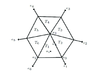
Figure 1: An illustration of the triangles containing $a_{1}$.

$$(\tilde{I}_{l}^{W}U_{\mu}-I_{l}^{W}\mu)(a_{1}) =\frac{U_{\mu}^{T_{1}}(a_{1})+\ldots+U_{\mu}^{T_{n_{a_{1}}}}(a_{1})}{|{\mathcal{T}}_{l}(a_{1})|}-\frac{{\mu}^{e_{1}}(a_{1})+\ldots+{\mu}^{e_{n_{a_{1}}}}(a_{1})}{|{\mathcal{T}}_{l}(a_{1})|}$$

$$=\frac{(U_{\mu}^{T_{1}}(a_{1})-{\mu}^{e_{1}}(a_{1}))+\ldots+(U_{\mu}^{T_{n_{a_{1}}}}(a_{1})-{\mu}^{e_{n_{a_{1}}}}(a_{1}))}{|{\mathcal{T}}_{l}(a_{1})|},$$

where $U_{\mu}^{T_{i}}$ and ${\mu}^{e_{i}},\ i=1,\ldots,{n_{a_{1}}}$, are the values of $U_{\mu}$ in $T_{i}$ and ${\mu}$ in $e_{i}$ respectively. ${n_{a_{1}}}$ is the number of elements which share the vertex $a_{1}$, specially for the case in Figure 1, ${n_{a_{1}}}=6$.

Since ${\mathcal{T}}_{l}$ is a sharp regular mesh,

$$\big{(}(\tilde{I}_{l}^{W}U_{\mu}-I_{l}^{W}\mu)(a_{1})\big{)}^{2} \lesssim\big{(}(U_{\mu}^{T_{1}}(a_{1})-{\mu}^{e_{1}}(a_{1}))\big{)}^{2}+\ldots+\big{(}(U_{\mu}^{T_{n_{a_{1}}}}(a_{1})-{\mu}^{e_{n_{a_{1}}}}(a_{1}))\big{)}^{2}$$

$$\lesssim h_{l}^{-1}\|U_{\mu}-\mu\|_{0,\partial{\mathcal{T}}_{l}(\Omega_{l}(a_{1}))}^{2},$$

where $\Omega_{l}(a_{1}):=\{T^{\prime}\in{\mathcal{T}}_{l},T^{\prime}\ {\rm{contains}}\ a_{1}\}$, $\partial{\mathcal{T}}_{l}(\Omega_{l}(a_{1})):=\bigcup_{T^{\prime}\in\Omega_{l}(a_{1})}\partial T^{\prime}$. Similarly we can get

$$\big{(}(\tilde{I}_{l}^{W}U_{\mu}-I_{l}^{W}\mu)(a_{2})\big{)}^{2}\lesssim h_{l}^{-1}\|U_{\mu}-\mu\|_{0,\partial{\mathcal{T}}_{l}(\Omega_{l}(a_{2}))}^{2},$$

and

$$\big{(}(\tilde{I}_{l}^{W}U_{\mu}-I_{l}^{W}\mu)(a_{3})\big{)}^{2}\lesssim h_{l}^{-1}\|U_{\mu}-\mu\|_{0,\partial{\mathcal{T}}_{l}(\Omega_{l}(a_{3}))}^{2}.$$

Then for the case $p=1$, (3.15) is proved. Suppose $a_{4}$ is the degree of freedom of $W(T_{1})$ in the edge $[a_{1},a_{3}]$, by the definition of $\tilde{I}_{l}^{W}$ and $I_{l}^{W}$, we have

$$(\tilde{I}_{l}^{W}U_{\mu}-I_{l}^{W}\mu)(a_{4})=\frac{(U_{\mu}^{T_{1}}(a_{4})-{\mu}(a_{4}))+(U_{\mu}^{T_{2}}(a_{4})-{\mu}(a_{4}))}{2},$$

which means

$$\big{(}(\tilde{I}_{l}^{W}U_{\mu}-I_{l}^{W}\mu)(a_{4})\big{)}^{2}\lesssim h_{l}^{-1}\|U_{\mu}-\mu\|_{0,\partial{\mathcal{T}}_{l}(\Omega_{l}(a_{4}))}^{2}.$$

Similarly we can obtain the estimates for the degrees of freedom of $W(T_{1})$ in the edges $[a_{1},a_{2}]$ and $[a_{2},a_{3}]$. Then for the case $p=2$, (3.15) is proved. Suppose $a_{i}$ is the degree of freedom of $W(T_{1})$ in the interior of $T_{1}$, since $\tilde{I}_{l}^{W}U_{\mu}(a_{i})=U_{\mu}(a_{i})$, according to the definition of $I_{l}^{W}\mu$, we can get

$$\tilde{I}_{l}^{W}U_{\mu}(a_{i})=I_{l}^{W}\mu(a_{i}).$$

Hence for the case $p\geq 3$, (3.15) is proved.

If $\partial T_{1}\cap\partial\Omega\not=\emptyset$, due to the fact that $\mu\in M_{l}^{0}$, (3.15) can be derived similarly. ∎

Remark 3.2.

From the proof of Lemma 3.1, we may see why we should define the degree of freedom in the interior of $T_{1}$ by $U_{\lambda}$ in the case $p\geq 3$. Actually, this definition may ensure (3.16), which is important in our analysis for the stability estimate of $I_{l}$.

Lemma 3.3.

For all $T\in{\mathcal{T}}_{l}$, $m\in L^{2}(\partial T)$, let $({{\boldsymbol{Q}}}_{m},U_{m})$ be the solution of the local problem (3.9-3.10). Then

$$\|{{\boldsymbol{Q}}}_{m}+\nabla U_{m}\|_{0,T}\lesssim h_{l}^{-1/2}\|U_{m}-m\|_{0,\partial T}.$$ (3.18)

Proof.

Applying the Green’s formula and using (3.9), we have

$$({{\boldsymbol{Q}}}_{m}+\nabla U_{m},{{\boldsymbol{v}}})_{T}=\langle U_{m}-m,{{\boldsymbol{v}}}\cdot{{\boldsymbol{n}}}\rangle_{\partial T},\quad\forall{{\boldsymbol{v}}}\in V(T).$$

Taking $v={{\boldsymbol{Q}}}_{m}+\nabla U_{m}$, and using Lemma 3.2 in [16], we get

$$\|{{\boldsymbol{Q}}}_{m}+\nabla U_{m}\|_{0,T}^{2} \leq\|U_{m}-m\|_{0,\partial T}\|{{\boldsymbol{Q}}}_{m}+\nabla U_{m}\|_{0,\partial T}$$

$$\lesssim h_{l}^{-1/2}\|U_{m}-m\|_{0,\partial T}\|{{\boldsymbol{Q}}}_{m}+\nabla U_{m}\|_{0,T},$$

Eliminating $\|{{\boldsymbol{Q}}}_{m}+\nabla U_{m}\|_{0,T}$ from both side of the above inequality concludes the proof. ∎

Lemma 3.4.

For all $\mu\in M_{l}^{0}$, we have

$$|I_{l}^{W}\mu|_{1,\Omega}^{2}\lesssim\hat{a}_{l}(\mu,\mu).$$

Proof.

By the triangle inequality and Lemma 3.1, we obtain

$$|I_{l}^{W}\mu|_{1,\Omega} \leq|I_{l}^{W}\mu-\tilde{I}_{l}^{W}U_{\mu}|_{1,\Omega}+|\tilde{I}_{l}^{W}U_{\mu}|_{1,\Omega},$$

$$\lesssim h_{l}^{-1/2}\|U_{\mu}-\mu\|_{0,\partial{\mathcal{T}}_{l}}+|\tilde{I}_{l}^{W}U_{\mu}|_{1,\Omega}.$$

The property of the operator $\tilde{I}_{l}^{W}$ (see Remark 3.2 of [4]) implies

$$|\tilde{I}_{l}^{W}U_{\mu}|_{1,\Omega} \lesssim|U_{\mu}|_{1,\Omega_{l}}+h_{l}^{-1/2}\|\llbracket U_{\mu}\rrbracket\|_{0,\mathcal{E}_{l}^{0}}$$

$$\lesssim|U_{\mu}|_{1,\Omega_{l}}+h_{l}^{-1/2}\|U_{\mu}-\mu\|_{0,\partial{\mathcal{T}}_{l}},$$

where $|v|_{1,\Omega_{l}}^{2}:=\sum_{T\in{\mathcal{T}}_{l}}|v|_{1,T}^{2},\ \forall v\in W_{l}$. Then using Lemma 3.3, we have

$$|U_{\mu}|_{1,\Omega_{l}}\lesssim\|{{\boldsymbol{Q}}}_{\mu}\|_{0,\Omega}+h_{l}^{-1/2}\|U_{\mu}-\mu\|_{0,\partial{\mathcal{T}}_{l}}.$$

Hence

$$|I_{l}^{W}\mu|_{1,\Omega}^{2}\lesssim\|{{\boldsymbol{Q}}}_{\mu}\|_{0,\Omega}^{2}+h_{l}^{-1}\|U_{\mu}-\mu\|_{0,\partial{\mathcal{T}}_{l}}^{2}\lesssim\hat{a}_{l}(\mu,\mu).$$

∎

Next, we prove the stability estimate of the intergrid transfer operator for the case $p=1$.

Lemma 3.5.

For the case $p=1$, let $({{\boldsymbol{Q}}}_{I_{l}\mu},U_{I_{l}\mu})\in{{\boldsymbol{V}}}(K)\times W(K)$ be the solution of the local problem (3.9-3.10) for any $K\in{\mathcal{T}}_{L}$, $I_{l}\mu\in L^{2}(\partial K)$, where $\mu\in M_{l}$. Then

$${{\boldsymbol{Q}}}_{I_{l}\mu}=-\nabla I_{l}^{W}\mu,\qquad U_{I_{l}\mu}=I_{l}^{W}\mu.$$ (3.19)

Proof.

The Green’s formula and (2.13) implies

$$(-\nabla I_{l}^{W}\mu,{{\boldsymbol{v}}})_{K}-(I_{l}^{W}\mu,{\rm div}\ {{\boldsymbol{v}}})_{K}=-\langle I_{l}^{W}\mu,{{\boldsymbol{v}}}\cdot{{\boldsymbol{n}}}\rangle_{\partial K}=-\langle I_{l}\mu,{{\boldsymbol{v}}}\cdot{{\boldsymbol{n}}}\rangle_{\partial K},$$

for all ${{\boldsymbol{v}}}\in{{\boldsymbol{V}}}(K)$. Since $I_{l}^{W}\mu$ is piecewise linear, then we have

$${\rm div}\ (-\nabla I_{l}^{W}\mu)=-\Delta I_{l}^{W}\mu=0,$$ (3.20)

which together with (2.13) yields

$$({\rm div}\ (-\nabla I_{l}^{W}\mu),w)_{K}+\tau_{L}\langle I_{l}^{W}\mu-I_{l}\mu,w\rangle_{\partial K}=0,\quad\forall w\in W(K).$$

Because the local problem (3.9-3.10) is uniquely solvable, we derive

$${{\boldsymbol{Q}}}_{I_{l}\mu}=-\nabla I_{l}^{W}\mu,\qquad U_{I_{l}\mu}=I_{l}^{W}\mu.$$

∎

Theorem 3.6.

When $p=1$, the intergrid transfer operator $I_{l}:M_{l}\rightarrow M_{L}$ satisfies

$$\hat{a}_{L}(I_{l}\mu,I_{l}\mu)\lesssim\hat{a}_{l}(\mu,\mu),\quad\forall\mu\in M_{l}^{0}.$$

Proof.

The definition of the bilinear form $\hat{a}_{L}(\cdot,\cdot)$, Lemma 3.5 and (2.13) yield

$$\hat{a}_{L}(I_{l}\mu,I_{l}\mu)=\sum_{K\in{\mathcal{T}}_{L}}\|{{\boldsymbol{Q}}}_{I_{l}\mu}\|_{0,K}^{2}=|I_{l}^{W}\mu|_{1,\Omega}^{2},$$

which, together with Lemma 3.4, implies the conclusion. ∎

For the case $p\geq 2$, since for all $v\in P_{p}(T)$, $\Delta v$ no longer equals to 0, which means Lemma 3.5 doesn’t hold any more. We will prove the stability estimate for $I_{l}$ through the estimation of terms $\|{{\boldsymbol{Q}}}_{I_{l}\mu}+\nabla I_{l}^{W}\mu\|_{0,\Omega}$ and $\|U_{I_{l}\mu}-I_{l}^{W}\mu\|_{0,\partial{\mathcal{T}}_{l}}$.

Lemma 3.7.

For all $T\in{\mathcal{T}}_{l}$, $f\in L^{2}(T)$, let $({{\boldsymbol{Q}}}_{f},U_{f})\in{{\boldsymbol{V}}}(T)\times W(T)$ be the solution of the local problem (3.11-3.12). Then

$$\|{{\boldsymbol{Q}}}_{f}\|_{0,T} \lesssim h_{l}\|f\|_{0,T},$$ (3.21)

$$\|U_{f}\|_{0,T}\lesssim h_{l}^{2}\|f\|_{0,T}, \quad\|U_{f}\|_{0,\partial T}\lesssim h_{l}^{3/2}\|f\|_{0,T}.$$ (3.22)

Proof.

Using the Green’s formula, we know there exists a $({{\boldsymbol{Q}}}_{f},U_{f})\in{{\boldsymbol{V}}}(T)\times W(T)$ such that

$$({{\boldsymbol{Q}}}_{f},{\boldsymbol{v}})_{T}-(U_{f},{\rm div}\ {{\boldsymbol{v}}})_{T}=0,$$ (3.23)

$$({\rm div}\ {{\boldsymbol{Q}}}_{f},w)_{T}+\tau_{l}\langle U_{f},w\rangle_{\partial T}=(f,w)_{T},$$ (3.24)

for all $({{\boldsymbol{v}}},w)\in{{\boldsymbol{V}}}(T)\times W(T)$.

Next we prove that for all $w\in P_{p}(T)$, there holds

$$\|w\|_{0,T}\lesssim h_{l}\frac{{\rm sup}_{{{\boldsymbol{v}}}\in V(T)}\ |\int_{T}w{\rm div}\ {{\boldsymbol{v}}}|}{\|{{\boldsymbol{v}}}\|_{0,T}}+h_{l}^{1/2}\|w\|_{0,\partial T}.$$ (3.25)

Supposing $\hat{T}$ is the standard triangle element, and $F_{T}:\hat{T}\rightarrow T$ is a linear map which is defined by $x=F_{T}(\hat{x}):=B_{T}\hat{x}+b$. A scalar function $w$ on $T$ is transformed to a scalar function $\hat{w}$ on $\hat{T}$ by $\hat{w}:=w\circ F_{T}(\hat{x})$, while for the vector function ${{\boldsymbol{v}}}$, we transform ${{\boldsymbol{v}}}$ to $\hat{{\boldsymbol{v}}}$ via $\hat{{\boldsymbol{v}}}:={\rm det}(B_{T})B_{T}^{-1}{{\boldsymbol{v}}}\circ F_{T}(\hat{x})$. We note that this is a divergence conserving transformation (see Lemma 3.59 in [21]), i.e.

$${\rm div}\ \hat{{\boldsymbol{v}}}={\rm det}(B_{T}){\rm div}\ {{\boldsymbol{v}}}.$$

Define

$$\|\hat{w}\|:=\frac{{\rm sup}_{\hat{{\boldsymbol{v}}}\in(P_{p}(\hat{T}))^{2}}|\int_{\hat{T}}\hat{w}{\rm div}\ \hat{{\boldsymbol{v}}}|}{\|\hat{{\boldsymbol{v}}}\|_{0,\hat{T}}}+\|\hat{w}\|_{0,\partial\hat{T}}.$$

Now we prove that $\|\cdot\|$ is a norm in the space $P_{p}(\hat{T})$. Apparently we have

$$\|c\hat{w}\|=|c|\ \|\hat{w}\|,$$

$$\|\hat{w}+\hat{u}\|\leq\|\hat{w}\|+\|\hat{u}\|,$$

for all $\hat{w},\ \hat{u}\in P_{p}(\hat{T})$ and $c\in\mathbb{R}$. Hence we only need to verify that if $\|\hat{w}\|=0$, then $w=0$.

If $\|\hat{w}\|=0$, by the definition of $\|\cdot\|$, we have

$$\int_{\hat{T}}\hat{w}\hat{u}_{p-1}=0,\quad\forall\hat{u}_{p-1}\in P_{p-1}(\hat{T}).$$

By Lemma A.1 in [8], we know

$$\|\hat{w}\|_{0,\hat{T}}\lesssim\|\hat{w}\|_{0,\hat{F}},\quad\forall\hat{F}\in\partial\hat{T}.$$

which implies $\hat{w}=0$. The scaling argument and the equivalence of the norms $\|\cdot\|_{0,\hat{T}}$ and $\|\cdot\|$ in the finite dimensional space $P_{p}(\hat{T})$ yield

$$h_{l}^{-1}\|w\|_{0,T} \lesssim\|\hat{w}\|_{0,\hat{T}}\lesssim\frac{{\rm sup}_{\hat{{\boldsymbol{v}}}\in(P_{p}(\hat{T}))^{2}}|\int_{\hat{T}}\hat{w}{\rm div}\ \hat{{\boldsymbol{v}}}|}{\|\hat{{\boldsymbol{v}}}\|_{0,\hat{T}}}+\|\hat{w}\|_{0,\partial\hat{T}}$$

$$\lesssim\frac{{\rm sup}_{{{\boldsymbol{v}}}\in V(T)}\ |\int_{T}w{\rm div}\ {{\boldsymbol{v}}}|}{\|{{\boldsymbol{v}}}\|_{0,T}}+h_{l}^{-1/2}\|w\|_{0,\partial T},$$

which results in (3.25). Taking ${{\boldsymbol{v}}}={{\boldsymbol{Q}}}_{f}$ in (3.23) and $w=U_{f}$ in (3.24), we can deduce

$$\|{{\boldsymbol{Q}}}_{f}\|_{0,T}^{2}+\tau_{l}\|U_{f}\|_{0,\partial T}^{2}=(f,U_{f})_{T}.$$ (3.26)

By (3.25) and (3.23), we get

$$\|U_{f}\|_{0,T} \lesssim h_{l}\frac{{\rm sup}_{{{\boldsymbol{v}}}\in V(T)}\ |\int_{T}U_{f}{\rm div}\ {{\boldsymbol{v}}}|}{\|{{\boldsymbol{v}}}\|_{0,T}}+h_{l}^{1/2}\|U_{f}\|_{0,\partial T}$$

$$\lesssim h_{l}\frac{{\rm sup}_{{{\boldsymbol{v}}}\in V(T)}\ |\int_{T}{{\boldsymbol{Q}}}_{f}{{\boldsymbol{v}}}|}{\|{{\boldsymbol{v}}}\|_{0,T}}+h_{l}^{1/2}\|U_{f}\|_{0,\partial T}$$

$$\lesssim h_{l}\|{{\boldsymbol{Q}}}_{f}\|_{0,T}+h_{l}^{1/2}\|U_{f}\|_{0,\partial T}.$$ (3.27)

Taking (3.27) to (3.26), and utilizing the Young’s inequality gives

$$\|{{\boldsymbol{Q}}}_{f}\|_{0,T}^{2}+\tau_{l}\|U_{f}\|_{0,\partial T}^{2} \lesssim\|f\|_{0,T}(h_{l}\|{{\boldsymbol{Q}}}_{f}\|_{0,T}+h_{l}^{1/2}\|U_{f}\|_{0,\partial T})$$

$$\leq C_{\delta}h_{l}^{2}\|f\|_{0,T}^{2}+\delta\|{{\boldsymbol{Q}}}_{f}\|_{0,T}^{2}+\delta h_{l}^{-1}\|U_{f}\|_{0,\partial T}^{2}.$$

Choosing $\delta<{\rm min}\ \{\frac{1}{2},\frac{1}{2}\tau_{l}h_{l}\}$, we obtain

$$\|{{\boldsymbol{Q}}}_{f}\|_{0,T}^{2}+\tau_{l}\|U_{f}\|_{0,\partial T}^{2}\lesssim h_{l}^{2}\|f\|_{0,T}^{2}.$$

Hence

$$\|{{\boldsymbol{Q}}}_{f}\|_{0,T}\lesssim h_{l}\|f\|_{0,T},\quad\|U_{f}\|_{0,\partial T}\lesssim h_{l}^{3/2}\|f\|_{0,T}.$$

By (3.27), we derive

$$\|U_{f}\|_{0,T}\lesssim h_{l}^{2}\|f\|_{0,T}.$$

∎

Now we are ready to prove the stability of the intergrid transfer operator for the case $p\geq 2$.

Theorem 3.8.

When $p\geq 2$, the intergrid transfer operator $I_{l}:M_{l}\rightarrow M_{L}$ satisfies

$$\hat{a}_{L}(I_{l}\mu,I_{l}\mu)\lesssim\hat{a}_{l}(\mu,\mu),\quad\forall\mu\in M_{l}^{0}.$$

Proof.

Let $({{\boldsymbol{Q}}}_{I_{l}\mu},U_{I_{l}\mu})\in{{\boldsymbol{V}}}(K)\times W(K)$ be the solution of the local problem (3.9-3.10) for any $K\in{\mathcal{T}}_{L}$, $I_{l}\mu\in L^{2}(\partial K)$. Then using the Green’s formula, we know that there exists a $({{\boldsymbol{Q}}}_{I_{l}\mu},U_{I_{l}\mu})\in{{\boldsymbol{V}}}(K)\times W(K)$ such that

$$({{\boldsymbol{Q}}}_{I_{l}\mu},{\boldsymbol{v}})_{K}-(U_{I_{l}\mu},{\rm div}\ {{\boldsymbol{v}}})_{T}=-\langle I_{l}\mu,{{\boldsymbol{v}}}\cdot{{\boldsymbol{n}}}\rangle_{\partial K},$$ (3.28)

$$({\rm div}\ {{\boldsymbol{Q}}}_{I_{l}\mu},w)_{K}+\tau_{L}\langle U_{I_{l}\mu}-I_{l}\mu,w\rangle_{\partial K}=0,$$ (3.29)

for all $({{\boldsymbol{v}}},w)\in{{\boldsymbol{V}}}(K)\times W(K)$. The Green’s formula and (2.13) imply

$$(-\nabla I_{l}^{W}\mu,{{\boldsymbol{v}}})_{K}-(I_{l}^{W}\mu,{\rm div}\ {{\boldsymbol{v}}})_{K}=-\langle I_{l}^{W}\mu,{{\boldsymbol{v}}}\cdot{{\boldsymbol{n}}}\rangle_{\partial K}=-\langle I_{l}\mu,{{\boldsymbol{v}}}\cdot{{\boldsymbol{n}}}\rangle_{\partial K},$$ (3.30)

$$({\rm div}\ (-\nabla I_{l}^{W}\mu),w)_{K}+\tau_{L}\langle I_{l}^{W}\mu-I_{l}\mu,w\rangle_{\partial K}=(-\Delta I_{l}^{W}\mu,w)_{K},$$ (3.31)

for all $({{\boldsymbol{v}}},w)\in{{\boldsymbol{V}}}(K)\times W(K)$. Denote $e_{{{\boldsymbol{Q}}}}={{\boldsymbol{Q}}}_{I_{l}\mu}+\nabla I_{l}^{W}\mu$ and $e_{U}=U_{I_{l}\mu}-I_{l}^{W}\mu$. Then $(e_{{{\boldsymbol{Q}}}},e_{U})\in{{\boldsymbol{V}}}(K)\times W(K)$ satisfy

$$(e_{{{\boldsymbol{Q}}}},{\boldsymbol{v}})_{K}-(e_{U},{\rm div}\ {{\boldsymbol{v}}})_{K}=0,$$ (3.32)

$$({\rm div}\ e_{{{\boldsymbol{Q}}}},w)_{K}+\tau_{L}\langle e_{U},w\rangle_{\partial K}=(\Delta I_{l}^{W}\mu,w)_{K},$$ (3.33)

for all $({{\boldsymbol{v}}},w)\in{{\boldsymbol{V}}}(K)\times W(K)$. By Lemma 3.7, we get

$$\|e_{{{\boldsymbol{Q}}}}\|_{0,K}\lesssim h_{L}\|\Delta I_{l}^{W}\mu\|_{0,K},$$

$$\|e_{U}\|_{0,K}\lesssim h_{L}^{2}\|\Delta I_{l}^{W}\mu\|_{0,K},$$

$$\|e_{U}\|_{0,\partial K}\lesssim h_{L}^{3/2}\|\Delta I_{l}^{W}\mu\|_{0,K}.$$

Summing up for all $K\in{\mathcal{T}}_{L}$ and utilizing the inverse inequality, we have

$$\|e_{{{\boldsymbol{Q}}}}\|_{0,\Omega}\lesssim\frac{h_{L}}{h_{l}}|I_{l}^{W}\mu|_{1,\Omega}\lesssim|I_{l}^{W}\mu|_{1,\Omega},$$ (3.34)

$$\|e_{U}\|_{0,\Omega}\lesssim\frac{h_{L}^{2}}{h_{l}}|I_{l}^{W}\mu|_{1,\Omega}\lesssim h_{L}|I_{l}^{W}\mu|_{1,\Omega},$$ (3.35)

$$\|e_{U}\|_{0,\partial{\mathcal{T}}_{L}}\lesssim\frac{h_{L}^{3/2}}{h_{l}}|I_{l}^{W}\mu|_{1,\Omega}\lesssim h_{L}^{1/2}|I_{l}^{W}\mu|_{1,\Omega}.$$ (3.36)

Then we can deduce

$$\|{{\boldsymbol{Q}}}_{I_{l}\mu}\|_{0,\Omega}\lesssim|I_{l}^{W}\mu|_{1,\Omega}+\|e_{{{\boldsymbol{Q}}}}\|_{0,\Omega}\lesssim|I_{l}^{W}\mu|_{1,\Omega}$$

and

$$\|U_{I_{l}\mu}-I_{l}\mu\|_{0,\partial{\mathcal{T}}_{L}}=\|e_{U}\|_{0,\partial{\mathcal{T}}_{L}}.$$

Hence

$$\hat{a}_{L}(I_{l}\mu,I_{l}\mu) =\|{{\boldsymbol{Q}}}_{I_{l}\mu}\|_{0,\Omega}^{2}+\tau_{L}\|U_{I_{l}\mu}-I_{l}\mu\|_{0,\partial{\mathcal{T}}_{L}}^{2}$$

$$\lesssim|I_{l}^{W}\mu|_{1,\Omega}^{2}+\tau_{L}h_{L}|I_{l}^{W}\mu|_{1,\Omega}^{2}$$

$$\lesssim|I_{l}^{W}\mu|_{1,\Omega}^{2},$$

which, together with Lemma 3.4, complete the proof. ∎

Remark 3.9.

In this paper, the proof of the stability estimate of the intergrid transfer operator is specified in meshes consisting of triangles, but we should mention that it can be extended to the meshes constituted with rectangles, tetrahedra or hexahedra.

4 Local Fourier analysis (LFA)

In this section, LFA will be used to give a quantitative insight of the convergence of Algorithm 2.1 in 1D case. For simplicity, in this section we focus on the analysis for the HDG discretization based on linear polynomial (P1) approximation (HDG-P1). We mainly consider the analysis of two level method of Algorithm 2.1. The LFA of three level method is also mentioned. The analysis imply the efficiency of Algorithm 2.1. We adopt the notations and philosophy in [22].

There are some necessary simplifications in the framework of LFA: the boundary conditions are neglected and the problem is considered on regular indefinite grids ${\mathcal{G}}_{h}=\{x:x=x_{j}=jh,j\in\mathbb{Z}\}$. It seems to be very restrictive and very unrealistic since the Robin boundary condition (1.3) and other absorbing boundary conditions are often applied in realistic Helmholtz problem, the neglect of boundary conditions does usually not affect the validity of LFA (cf. [22]).

For a fixed point $x\in{\mathcal{G}}_{h}$ and any infinite grid function $u_{h}$, we can define an operator ${\boldsymbol{L}}_{h}$ on the space of infinite grid functions by

$${\boldsymbol{L}}_{h}u_{h}(x)=\sum_{j\in J}l_{j}u_{h}(x+jh),$$

with stencil coefficients $l_{j}$ and a certain finite subset $J\subset\mathbb{Z}$. ${\boldsymbol{L}}_{h}=[l_{j}]_{h},j\in J$ is a stencil representation of ${\boldsymbol{L}}_{h}$. This formulation is particularly convenient in the context of LFA. It can be easily seen that the eigenfunctions of ${\boldsymbol{L}}_{h}$ are given by $\varphi_{h}(\theta,x)=e^{{\bf i}\theta x/h}$ with $x\in{\mathcal{G}}_{h}$ and $\theta\in\mathbb{R}$. In fact, the frequency $\theta$ can be restricted to the interval $(-\pi,\pi]$ as a fact that $\varphi_{h}(\theta+2\pi,x)=\varphi_{h}(\theta,x)$. These eigenfunctions are called Fourier components associated with a Fourier frequency $\theta$. The corresponding eigenvalues of ${\boldsymbol{L}}_{h}$ which are called Fourier symbols read as $\widetilde{{\boldsymbol{L}}}_{h}(\theta)=\sum_{j\in J}l_{j}e^{{\bf i}\theta j}$, and satisfy the following equality

$${\boldsymbol{L}}_{h}\varphi_{h}(\theta,x)=\widetilde{{\boldsymbol{L}}}_{h}(\theta)\varphi_{h}(\theta,x),\qquad x\in{\mathcal{G}}_{h},\theta\in(-\pi,\pi].$$ (4.1)

Given a so-called low frequency $\theta^{0}\in\Theta_{\rm low}:=(-\pi/2,\pi/2]$, its complementary frequency $\theta^{1}$ is defined as

$$\theta^{1}=\theta^{0}-{\rm sign}(\theta^{0})\pi.$$ (4.2)

It is appropriate to divide the Fourier space into the following two dimensional subspace

$$E_{2h}^{\theta^{0}}:={\rm span}\{\varphi_{h}(\theta^{0},x),\varphi_{h}(\theta^{1},x)\},$$ (4.3)

where the Fourier components $\varphi_{h}(\theta^{0},x)$ and $\varphi_{h}(\theta^{1},x)$ are called $2h$-harmonics. The definition of the $2h$-harmonics is motivated by the fact that each low frequency $\theta^{0}\in\Theta_{\rm low}$ is coupled with $\theta^{1}$ in the transition from ${\mathcal{G}}_{h}$ to ${\mathcal{G}}_{2h}$. Indeed they coincide with each other on the coarse grid. Interpreting the Fourier components as coarse grid functions yields

$$\varphi_{h}(\theta^{0},x)=\varphi_{2h}(2\theta^{0},x)=\varphi_{2h}(2\theta^{1},x)=\varphi_{h}(\theta^{1},x),\qquad\theta^{0}\in\Theta_{\rm low},\ x\in{\mathcal{G}}_{2h}.$$

A crucial observation is that the space $E_{2h}^{\theta^{0}}$ is invariant under both smoothing operators and correction schemes for general cases by two level method. The invariance property holds for many well-known smoothing methods (cf. [22]), such as Jacobi relaxation, lexicographical Gauss-Seidel relaxation, et al.

The main goal of LFA is to estimate the spectral radius or certain norms of the $k$-level operator. Let ${\boldsymbol{M}}_{h}$ be a discrete two level operator. In the following we will show that a block-diagonal representation for ${\boldsymbol{M}}_{h}$ consists of $2\times 2$ blocks $\widetilde{{\boldsymbol{M}}}_{h}(\theta)$ (cf. [22]), which denotes the representation of ${\boldsymbol{M}}_{h}$ on $E_{2h}^{\theta^{0}}$. Then the convergence factor of ${\boldsymbol{M}}_{h}$ by the LFA is defined as follows:

$$\rho({\boldsymbol{M}}_{h}):={\rm sup}\{\rho(\widetilde{{\boldsymbol{M}}}_{h}(\theta)):\ \theta\in\Theta_{\rm low}\},$$

where $\rho(\widetilde{{\boldsymbol{M}}}_{h}(\theta))$ is the spectral radius of the matrix $\widetilde{{\boldsymbol{M}}}_{h}(\theta)$. The generalizations to $k$-level analysis are shown in [22].

4.1 One dimensional Fourier symbols

In this subsection, we give the Fourier symbols of different operators in multilevel method for the HDG-P1 discretization for one dimensional Helmholtz equation. Since the boundary condition is neglected in the LFA, the stencil presentation of discretization operator ${\boldsymbol{A}}_{h}$ from (2.12) can be derived as

$${\boldsymbol{A}}_{h}=[s_{1}\ \ s_{0}\ \ s_{1}]_{h},$$

where

$$s_{1}=\frac{1}{t}\Big{(}\frac{\sigma_{2}}{t\sigma_{1}}-\frac{\sigma_{2}(3t^{2}{\bf i}+18)}{(18t-t^{3})\sigma_{1}}\Big{)}-\frac{-2t^{4}{\bf i}+12t^{2}{\bf i}+72+136{\bf i}}{t^{5}-24t^{3}+148t}-\frac{6t^{2}-72+12{\bf i}}{t^{5}-24t^{3}+148t},$$

and

$$s_{0} =-\frac{1}{t}\Big{(}\frac{\sigma_{3}}{\sigma_{4}}-\frac{-4t^{7}{\bf i}+t^{5}(20+84{\bf i})+t^{3}(-432-480{\bf i})+t(2736+432{\bf i})}{t(t^{8}-24t^{6}+184t^{4}-864t^{2}+5328)}+1\Big{)}$$

$$\quad-\frac{-4t^{4}{\bf i}+60t^{2}{\bf i}+72-160{\bf i}}{t^{5}-24t^{3}+148t}-\frac{\sigma_{3}}{t\sigma_{4}},$$

here $t=kh$, and

$$\sigma_{1}=t^{4}{\bf i}+t^{2}(8-12{\bf i})-72-12{\bf i},\quad\sigma_{2}=36t-2t^{3},$$

$$\sigma_{3}=6t^{2}-72+12{\bf i},\quad\sigma_{4}=t^{4}-24t^{2}+148.$$

Combining the above expression and (4.1) yields the Fourier symbol of ${\boldsymbol{A}}_{h}$ as

$$\widetilde{{\boldsymbol{A}}}_{h}(\theta)=2s_{1}\cos{\theta}+s_{0}.$$ (4.4)

For simplicity, we use standard weighted Jacobi ($\omega$-JAC) and lexicographical Gauss-Seidel (GS-LEX) relaxations as the smoothers in the LFA. It is easy to derive the weighted Jacobi relaxation matrix as ${\boldsymbol{S}}^{J}_{h}={\boldsymbol{I}}_{h}-\omega{\boldsymbol{D}}^{-1}_{h}{\boldsymbol{A}}_{h}$, where ${\boldsymbol{I}}_{h}$ is indentity matrix, ${\boldsymbol{D}}_{h}$ consists of the diagonal of ${\boldsymbol{A}}_{h}$ and $\omega$ is a weighted parameter. Due to the fact that ${\boldsymbol{D}}_{h}=s_{0}{\boldsymbol{I}}_{h}$, one can easily deduce the Fourier symbol of weighted Jacobi relaxation as follows:

$$\widetilde{{\boldsymbol{S}}}^{J}_{h}(\theta)=1-\frac{2\omega}{s_{0}}(s_{1}\cos{\theta}+\frac{s_{0}}{2}).$$ (4.5)

The GS-LEX relaxation matrix is ${\boldsymbol{S}}^{GS}_{h}=({\boldsymbol{D}}_{h}-{\boldsymbol{L}}_{h})^{-1}{\boldsymbol{U}}_{h}$, where $-{\boldsymbol{L}}_{h}$ is the strictly lower triangular part of ${\boldsymbol{A}}_{h}$ and $-{\boldsymbol{U}}_{h}$ is the strictly upper triangular part of ${\boldsymbol{A}}_{h}$. The Fourier symbol of ${\boldsymbol{S}}^{GS}_{h}$ can also be directly derived that

$$\widetilde{{\boldsymbol{S}}}^{GS}_{h}(\theta)=-\frac{s_{1}e^{{\bf i}\theta}}{s_{1}e^{{\bf-i}\theta}+s_{0}}.$$ (4.6)

Note that for the restriction matrix ${\boldsymbol{I}}^{2h}_{h}=[r_{j}]^{2h}_{h}$ and $x\in{\mathcal{G}}_{2h}$, there holds

$$({\boldsymbol{I}}^{2h}_{h}\varphi_{h}(\theta^{\alpha},\cdot))(x)=\sum_{j\in J}r_{j}e^{{\bf i}j\theta^{\alpha}}\varphi_{h}(\theta^{\alpha},x)=\sum_{j\in J}r_{j}e^{{\bf i}j\theta^{\alpha}}\varphi_{2h}(2\theta^{0},x),\qquad\alpha=0,1.$$

By an analogous stencil argument, the stencil presentation of full weighting restriction matrix for the HDG-P1 discretization system in one dimensional case is derived to be ${\boldsymbol{I}}^{2h}_{h}=[1/4,1/2,1/4]_{h}^{2h}$. Thus, the Fourier symbol of ${\boldsymbol{I}}^{2h}_{h}$ can be deduced as

$$\widetilde{{\boldsymbol{I}}}^{2h}_{h}(\theta)=\frac{1}{2}(1+\cos{\theta}).$$

For the linear prolongation matrix ${\boldsymbol{I}}^{h}_{2h}$ which is defined as

$$({\boldsymbol{I}}^{h}_{2h}\varphi_{2h}(2\theta^{0},\cdot))(x)=\varphi_{2h}(2\theta^{0},x)=\varphi_{h}(\theta^{0},x),\qquad x\in{\mathcal{G}}_{2h},\theta^{0}\in\Theta_{\rm low},$$

$$({\boldsymbol{I}}^{h}_{2h}\varphi_{2h}(2\theta^{0},\cdot))(x)=\frac{1}{2}(\varphi_{h}(\theta^{0},x-h)+\varphi_{h}(\theta^{0},x+h)),\qquad x\in{\mathcal{G}}_{h}\setminus{\mathcal{G}}_{2h},\theta^{0}\in\Theta_{\rm low},$$

one can also obtain its Fourier symbol as follows (cf. [22]):

$$\widetilde{{\boldsymbol{I}}}^{h}_{2h}(\theta)=\frac{1}{2}(1+\cos{\theta}).$$

4.2 Smoothing analysis

Since every two dimensional subspace of $2h$-harmonics $E^{\theta^{0}}_{2h}$ with $\theta^{0}\in\Theta_{\rm low}$ is left invariant under the $\omega$-JAC and GS-LEX relaxations, then the Fourier representation of smoother ${\boldsymbol{S}}_{h}={\boldsymbol{S}}^{J}_{h}$ or ${\boldsymbol{S}}^{GS}_{h}$ with respect to $E_{2h}^{\theta^{0}}$ can be written as

$$\left[\begin{array}[]{cc}\widetilde{{\boldsymbol{S}}}_{h}(\theta^{0})&0\\ 0&\widetilde{{\boldsymbol{S}}}_{h}(\theta^{1})\\ \end{array}\right],$$ (4.7)

where $\widetilde{{\boldsymbol{S}}}_{h}(\theta)$ is the smoother symbol derived in (4.5) and (4.6). The spectral radius of the smoother operator can be easily calculated since the above matrix is diagonal.

We concern on the LFA for HDG-P1 method. The left graph of Figure 2 shows the Fourier symbols $\widetilde{{\boldsymbol{S}}}^{J}_{h}(\theta)$ for $\omega$-JAC smoother with $\omega=0.6$. We find that $\widetilde{{\boldsymbol{S}}}^{J}_{h}(\theta)\geq 1$ always occur at the low frequencies, and small $t$ leads to a better relaxation. Similar phenomenon is also observed for GS-LEX smoother in the right graph of Figure 2. Thus, for fixed wave number $\kappa$, both $\omega$-JAC and GS-LEX relaxations can be used as smoother on fine grids, but on coarse grids they may amplify the error.

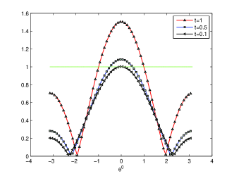
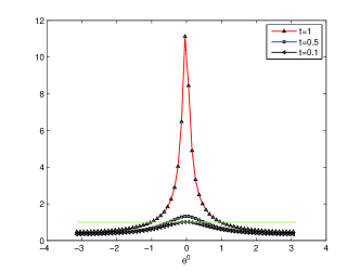
Figure 2: $|\widetilde{{\boldsymbol{S}}}^{J}_{h}(\theta)|$ with $\omega=0.6$ (left) and $|\widetilde{{\boldsymbol{S}}}^{GS}_{h}(\theta)|$ (right) over $(-\pi,\pi]$ for $t=0.1,0.5,1$.

Motivated by the idea in [9], we use GMRES smoothing on coarse grids. Unfortunately, since the GMRES smoothing is nonlinear in the starting value, its Fourier symbol can not be derived. In the following, we will give some explanations for the performance of GMRES smoothing from the numerical point of view.

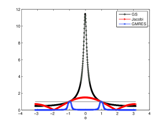
Figure 3: Amplification factor of GS, Jacobi and GMRES smoothing for $t=1$.

For the ease of presentation, we restrict ourselves to the one dimensional Helmholtz equation on an interval $(0,10)$ with homogeneous Dirichlet boundary conditions. For $\kappa=200$, we apply the grid with mesh size $h=0.005$, i.e., $t=1$. Let the vector $u_{0}=e^{{\bf i}\theta{\boldsymbol{x}}/h}$ be an initial choice for smoothing, where ${\boldsymbol{x}}=[x_{1},\cdots,x_{N-1}],x_{k}=x_{k-1}+kh,x_{0}=0,k=1,\cdots,N-1$, $N=10/h-1$, $\theta\in(-\pi,\pi]$. We assume that ${\boldsymbol{S}}_{h}$ is the relaxation iteration matrix and $u_{1}={\boldsymbol{S}}_{h}u_{0}$ is the new vector after one step of smoothing. Then for fixed $\theta$, we obtain the amplification factor for one step of smoothing $\rho_{s}(\theta)=\|u_{1}\|/\|u_{0}\|$, where $\|\cdot\|$ stands for the Euclidean norm. We can see from Figure 3, the amplification factor of GMRES relaxation is always smaller than that of GS and Jacobi relaxations. When the other two smoothers fail, the GMRES relaxation can still lead to convergence. Hence, we replace them with GMRES smoothing on coarse grids.

4.3 Two and three level local Fourier analysis

We have briefly characterized the smoothing procedure in the multilevel algorithm, in this subsection, the influence of coarse grid correction will be taken into account. We will focus on the LFA of two level method and concisely mention the three level method. For simplicity, we consider the two and three level methods without post-smoothing and with one step of smoothing on each level. Since the Fourier symbol can not be obtained for GMRES smoothing, we only consider the two and three level methods with $\omega$-JAC or GS-LEX relaxation. Then the iteration operator of Algorithm 2.1 in this simple case can be derived as $(I-T_{L})\cdots(I-T_{0}),$ where $T_{l}=\mu_{l}I_{l}R_{l}A_{l}P_{l}$, $R_{l}$ is smoothing operator.

For the two level method, the iteration matrix is given by

$${\boldsymbol{M}}_{2}=\Big{(}{\boldsymbol{I}}_{1}-\mu_{1}({\boldsymbol{I}}_{1}-{\boldsymbol{S}}_{1})\Big{)}\Big{(}{\boldsymbol{I}}_{1}-\mu_{0}{\boldsymbol{I}}^{1}_{0}({\boldsymbol{A}}_{0})^{-1}{\boldsymbol{I}}^{0}_{1}{\boldsymbol{A}}_{1}\Big{)}.$$

Here, for $l\geq 0$, ${\boldsymbol{S}}_{l}={\boldsymbol{I}}_{l}-{\boldsymbol{R}}_{l}{\boldsymbol{A}}_{l}$ is smoothing relaxation matrix, ${\boldsymbol{I}}_{l}$ with the same size as ${\boldsymbol{A}}_{l}$ is identity matrix , ${\boldsymbol{I}}^{s}_{l}(s>l)$ is prolongation matrix from level $l$ to $s$, ${\boldsymbol{I}}^{s}_{l}(s<l)$ is restriction matrix from level $l$ to $s$, and ${\boldsymbol{R}}_{l}$ stands for matrix representation of smoother $R_{l}$.

Since every two dimensional subspace (4.3) of $2h$-harmonics $E^{\theta^{0}}_{2h_{1}}$ with $\theta^{0}\in(-\pi/2,\pi/2]$ is left invariant under $\omega$-JAC or GS-LEX smoothing operator and correction operator, the representation of two level iteration matrix of ${\boldsymbol{M}}_{2}$ on $E^{\theta^{0}}_{2h_{1}}$ is given by a $2\times 2$ matrix as follows:

$$\widetilde{{\boldsymbol{M}}}_{2} = \left[\widetilde{{\boldsymbol{I}}}_{1}-\mu_{1}\left(\widetilde{{\boldsymbol{I}}}_{1}-\left[\begin{array}[]{c}\widetilde{{\boldsymbol{S}}}_{1}(\theta^{0})\\ \widetilde{{\boldsymbol{S}}}_{1}(\theta^{1})\\ \end{array}\right]_{D}\right)\right]$$ (4.17)

$$\cdot\left[\widetilde{{\boldsymbol{I}}}_{1}-\mu_{0}\left[\begin{array}[]{c}\widetilde{{\boldsymbol{I}}}_{0}^{1}(\theta^{0})\\ \widetilde{{\boldsymbol{I}}}_{0}^{1}(\theta^{1})\\ \end{array}\right]\widetilde{{\boldsymbol{A}}}_{0}(2\theta^{0})^{-1}\left[\begin{array}[]{c}\widetilde{{\boldsymbol{I}}}_{1}^{0}(\theta^{0})\\ \widetilde{{\boldsymbol{I}}}_{1}^{0}(\theta^{1})\\ \end{array}\right]^{t}\left[\begin{array}[]{c}\widetilde{{\boldsymbol{A}}}_{1}(\theta^{0})\\ \widetilde{{\boldsymbol{A}}}_{1}(\theta^{1})\\ \end{array}\right]_{D}\right].$$

where $\widetilde{{\boldsymbol{I}}}_{1}$ is $2\times 2$ identity matrix and the subscript-_D denotes the transformation of a vector into a diagonal matrix. Then the spectral radius of $\widetilde{{\boldsymbol{M}}}_{2}$ for different $\theta^{0}\in\Theta_{\rm low}$ can be obtained analytically and numerically.

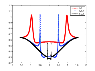
Figure 4: $\rho(\widetilde{{\boldsymbol{M}}}_{2})$ with $\omega=0.6$ over $\theta^{0}\in\Theta_{\rm low}$ for $t=1$, $t=0.5$ and $t=0.1$.

Figure 4 shows the spectral radius of $\widetilde{{\boldsymbol{M}}}_{2}$ with $\omega=0.6$ over $\theta^{0}\in\Theta_{\rm low}$ under $\omega$-JAC relaxation for different mesh size $t$ on the finest grid. If no confusion is possible, we will always denote $t=$constant for $t=\kappa h_{L}$ on the finest grid. We observe that when $t=1$, for most of the frequencies $\theta^{0}\in\Theta_{\rm low}$ the amplification factor is smaller than 1. The amplification factor tends to larger than 1 only under a few frequencies. Actually, the appearance of such a resonance is caused by the coarse grid correction and originates from the inversion of the coarse grid discretization symbol $\widetilde{{\boldsymbol{A}}}_{0}(2\theta^{0})$ in (4.17). Based on this reason, the coarsest grid is chosen to satisfies the mesh condition $\kappa h/p\leq 2$ in our algorithm. The good performance of two level method for $t=0.5$ and $t=0.1$ indicates that when the mesh is fine enough to capture the character of solution, standard smoother works out. We will utilize the GMRES smoothing when $\kappa h/p\geq 0.5$ and perform weighted Jacobi or Gauss-Seidel smoothing on those relatively fine grids.

The main idea of the three level analysis is to recursively apply the previous two level analysis. First, we define the four dimensional $4h$-harmonics by

$$E_{4h_{2}}^{\theta^{0}}:={\rm span}\{\varphi_{h_{2}}(\theta^{00},x),\varphi_{h_{2}}(\theta^{01},x),\varphi_{h_{2}}(\theta^{10},x),\varphi_{h_{2}}(\theta^{11},x)\},$$

where $\theta^{\alpha 0}=\frac{\theta^{\alpha}}{2},\theta^{\alpha 1}=\frac{\theta^{\alpha}}{2}-{\rm sign}(\frac{\theta^{\alpha}}{2})\pi,\alpha=0,1$. Similar to the two level method, the iteration matrix can be deduced to be

$${\boldsymbol{M}}_{3}=\Big{(}{\boldsymbol{I}}_{2}-\mu_{2}({\boldsymbol{I}}_{2}-{\boldsymbol{S}}_{2})\Big{)}\Big{(}{\boldsymbol{I}}_{2}-\mu_{1}{\boldsymbol{I}}^{2}_{1}({\boldsymbol{I}}_{1}-{\boldsymbol{S}}_{1})({\boldsymbol{A}}_{1})^{-1}{\boldsymbol{I}}^{1}_{2}{\boldsymbol{A}}_{2}\Big{)}\Big{(}{\boldsymbol{I}}_{2}-\mu_{0}{\boldsymbol{I}}^{2}_{0}({\boldsymbol{A}}_{0})^{-1}{\boldsymbol{I}}^{0}_{2}{\boldsymbol{A}}_{2}\Big{)}.$$

It is easy to see that the three level operator leaves the space of $4h$-harmonics $E_{4h_{2}}^{\theta^{0}}$ invariant (cf. [22]) for any $\theta^{0}\in\Theta_{\rm low}$. This yields a block diagonal representation of ${\boldsymbol{M}}_{3}$ with the following $4\times 4$ matrix $\widetilde{{\boldsymbol{M}}}_{3}$:

$$\widetilde{{\boldsymbol{M}}}_{3} = \left[\widetilde{{\boldsymbol{I}}}_{2}-\mu_{2}\left(\widetilde{{\boldsymbol{I}}}_{2}-\widetilde{{\boldsymbol{S}}}_{2}(\theta)\right)\right]$$

$$\cdot\left[\widetilde{{\boldsymbol{I}}}_{2}-\mu_{1}\widetilde{{\boldsymbol{I}}}_{1}^{2}(\theta)\left(\widetilde{{\boldsymbol{I}}}_{1}-\left[\begin{array}[]{c}\widetilde{{\boldsymbol{S}}}_{1}(\theta^{0})\\ \widetilde{{\boldsymbol{S}}}_{1}(\theta^{1})\\ \end{array}\right]_{D}\right)\left[\begin{array}[]{cc}\widetilde{{\boldsymbol{A}}}_{1}(\theta^{0})\\ \widetilde{{\boldsymbol{A}}}_{1}(\theta^{1})\\ \end{array}\right]_{D}^{-1}(\widetilde{{\boldsymbol{I}}}_{2}^{1}(\theta))^{t}\widetilde{{\boldsymbol{A}}}_{2}(\theta)\right]$$

$$\cdot\left[\widetilde{{\boldsymbol{I}}}_{2}-\mu_{0}\widetilde{{\boldsymbol{I}}}_{1}^{2}(\theta)\widetilde{{\boldsymbol{I}}}_{0}^{1}(\theta)\widetilde{{\boldsymbol{A}}}_{0}(2\theta^{0})^{-1}(\widetilde{{\boldsymbol{I}}}_{1}^{0}(\theta))^{t}(\widetilde{{\boldsymbol{I}}}_{2}^{1}(\theta))^{t}\widetilde{{\boldsymbol{A}}}_{2}(\theta)\right],$$

where $\widetilde{{\boldsymbol{I}}}_{2}$ is $4\times 4$ identity matrix, $\widetilde{{\boldsymbol{S}}}_{2}(\theta)=\left[\begin{array}[]{cc}\widetilde{{\boldsymbol{S}}}_{2}(\theta^{00})\\ \widetilde{{\boldsymbol{S}}}_{2}(\theta^{01})\\ \widetilde{{\boldsymbol{S}}}_{2}(\theta^{10})\\ \widetilde{{\boldsymbol{S}}}_{2}(\theta^{11})\\ \end{array}\right]_{D}$, $\widetilde{{\boldsymbol{A}}}_{2}(\theta)=\left[\begin{array}[]{cc}\widetilde{{\boldsymbol{A}}}_{2}(\theta^{00})\\ \widetilde{{\boldsymbol{A}}}_{2}(\theta^{01})\\ \widetilde{{\boldsymbol{A}}}_{2}(\theta^{10})\\ \widetilde{{\boldsymbol{A}}}_{2}(\theta^{11})\\ \end{array}\right]_{D}$, $\widetilde{{\boldsymbol{I}}}_{1}^{2}(\theta)=\left[\begin{array}[]{cc}\widetilde{{\boldsymbol{I}}}_{1}^{2}(\theta^{00})\quad 0\\ \widetilde{{\boldsymbol{I}}}_{1}^{2}(\theta^{01})\quad 0\\ 0\quad\widetilde{{\boldsymbol{I}}}_{1}^{2}(\theta^{10})\\ 0\quad\widetilde{{\boldsymbol{I}}}_{1}^{2}(\theta^{11})\\ \end{array}\right]$, $\widetilde{{\boldsymbol{I}}}_{0}^{1}(\theta)=\left[\begin{array}[]{c}\widetilde{{\boldsymbol{I}}}_{0}^{1}(\theta^{0})\\ \widetilde{{\boldsymbol{I}}}_{0}^{1}(\theta^{1})\\ \end{array}\right]$, and $\widetilde{{\boldsymbol{I}}}_{2}^{1}(\theta),\widetilde{{\boldsymbol{I}}}_{1}^{0}(\theta)$ are defined similarly.

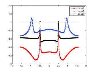
Figure 5: Case 1 (t=0.5): $\rho(\widetilde{{\boldsymbol{M}}}_{2})$ over $\theta^{0}\in\Theta_{\rm low}$, Case 2 (t=0.5) and Case 3 (t=0.25) denote for $\rho(\widetilde{{\boldsymbol{M}}}_{3})$.

It can be seen from Figure 5, when the mesh size on the coarsest grid is determined to be the same, the performance of two and three level methods behave similarly, although the two level method has smaller spectral radius. We also observe that a coarser initial grid used for ${\boldsymbol{M}}_{3}$ will deteriorate its convergence.

5 Numerical results

We will present two numerical examples to demonstrate Algorithm 2.1 in two dimension. Our multilevel algorithm is used as a preconditioner in outer GMRES iterations (PGMRES). The level $l$ which distinguishes the smoothing strategy satisfies $\kappa h_{l}/p\thickapprox 0.5$. We always use Gauss-Seidel relaxation when $\kappa h_{l}/p<0.5$ and GMRES relaxation otherwise in Algorithm 2.1. The smoothing step $\{m_{i}\}^{4}_{i=1}$ is chosen as two if there is no any annotation. At the $l$-th level, the discrete problem is ${\bf A}_{l}{\bf u}_{l}={\bf F}_{l}$. Let ${\bf r}^{n}_{l}={\bf F}_{l}-{\bf A}_{l}{\bf u}^{n}_{l}$ be the residual with respect to the $n$-th iteration. The PGMRES algorithm stops when

$$\|{\bf r}^{n}_{l}\|/\|{\bf r}^{0}_{l}\|\leq 10^{-6},$$

where $\|v\|$ is the $L^{2}$ norm of the vector $v$. The number of iteration steps required to achieve the desired accuracy is denoted by iter.

Example 5.1.

We consider a two dimensional Helmholtz equation with the first order absorbing boundary condition (cf. [17, 23]):

$$-\Delta u-\kappa^{2}u =f:=\frac{\sin(\kappa r)}{r}\quad{\rm in}\ \Omega,$$

$$\frac{\partial u}{\partial n}+{\rm i}\kappa u =g\quad{\rm on}\ \partial\Omega.$$

Here $\Omega$ is a unit square with center $(0,0)$ and $g$ is chosen such that the exact solution is

$$u=\frac{\cos(\kappa r)}{\kappa}-\frac{\cos\kappa+\rm i\sin\kappa}{\kappa(J_{0}(\kappa)+{\rm i}J_{1}(\kappa))}J_{0}(\kappa r),$$

where $J_{\nu}(z)$ are Bessel functions of the first kind.

Table 1: Iteration number of PGMRES based on Algorithm 2.1 for the HDG-P1 in the cases $\kappa=50,100,200$ with coarsest grid size $\kappa h_{0}/p\approx 2$.

$\kappa=50$	Level	3	4	5
	DOFs	98816	394240	1574912
	iter (P1)	20	16	15
$\kappa=100$	Level	3	4	5
	DOFs	394240	1574912	6295552
	iter (P1)	30	20	19
$\kappa=200$	Level	2	3	4
	DOFs	394240	1574912	6295552
	iter (P1)	76	54	35

Table 2: Iteration number of PGMRES based on Algorithm 2.1 for the HDG-P2 in the cases $\kappa=50,200,360$ with coarsest grid size $\kappa h_{0}/p\approx 2$.

$\kappa=50$	Level	3	4	5
	DOFs	37248	148224	591360
	iter (P1)	11	10	9
$\kappa=200$	Level	2	3	4
	DOFs	148224	591360	2362368
	iter (P1)	30	29	24
$\kappa=360$	Level	2	3	4
	DOFs	591360	2362368	9443328
	iter (P1)	30	31	25

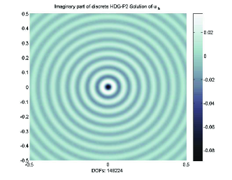
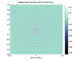
Figure 6: Surface plot of imaginary part of discrete HDG-P2 solutions for $\kappa=100$ (left) and $\kappa=200$ (right) on the grid with mesh condition $\kappa h/p\approx 0.55$ (left) and $1.1$ (right).

In this example, the coarsest level of multilevel method is chosen to satisfy $\kappa h_{0}/p\thickapprox 2$ for $\kappa\leq 360$. For $400\leq\kappa\leq 700$, we choose the coarsest grid condition with the same mesh size $h_{0}$ such that $\kappa h_{0}/p\thickapprox 1.1\thicksim 1.9$. We can observe from Table 1 and Table 2 that the iteration number is mesh independent for fixed $\kappa$, and it increases mildly with large wave number. We note that for the piecewise linear polynomial, HDG method does not have the advantage of saving degrees of freedom, while in the case of piecewise quadratic polynomial, the ratio between the number of degrees of freedom for HDG and standard DG method is about $\frac{3}{4}$. And the higher the polynomial degree is, the lower the ratio is. Hence we focus on HDG-P2 for the performance of our algorithm in this example.

Figure 6 displays the surface plot of imaginary part of discrete HDG-P2 solutions for $\kappa=100,200$ on the grid with mesh condition $\kappa h/p\approx 0.55$ and $1.1$ respectively. Indeed, the discrete solutions have correct shapes and amplitudes as the exact solutions. We also test the performance of PGMRES based on Algorithm 2.1 with different smoothing steps. Table 3 shows that when it takes two steps of smoothing the iteration number is much small with respect to one smoothing step. But the advantage of reducing the iteration number by adding more smoothing steps is deteriorating, and more steps of GMRES smoothing requires more memory to store data in the computation. Hence, in the following we will use two smoothing steps in Algorithm 2.1.

Table 3: Iteration number of PGMRES based on Algorithm 2.1 for HDG-P2 with different smoothing steps ($m_{i}=m,i=1,\cdots,4$, $\kappa=100$).

HDG-P2	Level	3	4	5
	DOFs	148224	591360	2362368
	iter ($m=1$)	30	27	21
	iter ($m=2$)	18	15	13
	iter ($m=3$)	15	13	11

Table 4: Iteration number of PGMRES based on Algorithm 2.1 for HDG-P2 in the cases $\kappa=400,500,600,700$.

HDG-P2	Level	2	3
	DOFs	2362368	9443328
	iter ($\kappa=400$)	11	11
	iter ($\kappa=500$)	16	16
	iter ($\kappa=600$)	26	27
	iter ($\kappa=700$)	45	50

Table 4 shows the iteration number of PGMRES based on Algorithm 2.1 for the cases $\kappa=400,500,600,700$ with the same coarsest grid $h_{0}\approx 0.00552$ such that $\kappa h_{0}/p\thickapprox 1.1\thicksim 1.9$, we can see that the iteration number is still stable and acceptable.

Example 5.2.

We consider a cave model in a unit square domain with center $(0,0)$. Figure 8 shows the computational domain and the variation of wave number in different subdomains which are indicated by different colors.

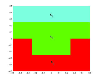
Figure 7: The computational domain of cave problem with different wave number indicated.

We denote by $\kappa_{3}=q_{2}\kappa_{2}=q_{1}\kappa_{1}$. The Robin boundary condition (1.3) is set to be $g=0$ and the external force $f(x)$ in (1.2) is a narrow Gaussian point source (cf. [11]) located at the center $(0,0)$:

$$f(x_{1},x_{2})=\frac{1}{{\rm i\kappa}}e^{-(\frac{4\kappa}{\pi})^{2}(x_{1}^{2}+x_{2}^{2})}.$$

Table 5: Iteration number of PGMRES based on Algorithm 2.1 for HDG-P1, HDG-P2 and HDG-P3 discretizations for the case $\kappa_{3}=200,q_{2}=2,q_{1}=3$.

HDG-P1	Level	2	3	4
	DOFs	221952	886272	3542016
	iter	166	129	54
HDG-P2	Level	2	3	4
	DOFs	83520	332928	1329408
	iter	53	66	54
HDG-P3	Level	2	3	4
	DOFs	197632	788480	3149824
	iter	23	26	26

For this problem we firstly test the performance of our multilevel method for HDG method with different polynomial order approximations. In Table 5, the iteration number for HDG-P1 and HDG-P2 are based on the coarsest grid condition with $\kappa_{3}h_{0}/p\thickapprox 2.95$. We can see that the multilevel method is more stable when the higher polynomial order approximation is applied. But for HDG-P3, the iteration number will be more than 200 with the above coarsest grid condition. Thus, we utilize the coarsest grid condition $\kappa_{3}h_{0}/p\thickapprox 1.47$ for HDG-P3, then the convergence of PGMRES becomes stable. Comparing the iteration number for HDG-P1 and HDG-P3, one can also observe that when the degrees of freedom are similar on each level, the convergence of PGMRES is more stable for higher polynomial order approximation. In the following, we focus on the performance of HDG-P2.

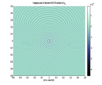
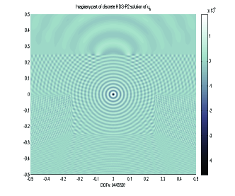
Figure 8: Surface plot of imaginary part of discrete HDG-P2 solutions for $\kappa_{3}=600,q_{2}=2,q_{1}=3$ (left) and $\kappa_{3}=600,q_{2}=2,q_{1}=10$ (right) on the grid with mesh condition $\kappa_{3}h/p\approx 0.4$.

Figure 8 displays the surface plot of imaginary part of discrete HDG-P2 solutions $u_{h}$ for $\kappa_{3}=600$ with $q_{2}=2,q_{1}=3$ and $q_{1}=10$ on the grid with mesh condition $\kappa_{3}h/p\approx 0.4$. The iteration number of PGMRES based on Algorithm 2.1 for different $\kappa_{3},q_{2}$ and $q_{1}$ are listed in Table 6. The larger jump of wave numbers between different subdomain will deteriorate the convergence of the algorithm. For instance, the iteration number for the case $q_{1}=10$ are much more than that for $q_{1}=3$. But for fixed $\kappa_{3},q_{2}$ and $q_{1}$, the iteration number are robust on different levels.

Table 6: Iteration number of PGMRES based on Algorithm 2.1 for HDG-P2 discretizations for the cases $\kappa_{3}=400$ $(q_{2}=2,q_{1}=3,q_{1}=10)$ and $\kappa_{3}=600$ $(q_{2}=2,q_{1}=3,q_{1}=10)$.

$\kappa=400$	Level	2	3
	DOFs	2362368	9443328
	iter $(q_{2}=2,q_{1}=3)$	14	14
	iter $(q_{2}=2,q_{1}=10)$	28	27
$\kappa=600$	Level	2	3
	DOFs	2362368	9443328
	iter $(q_{2}=2,q_{1}=3)$	24	26
	iter $(q_{2}=2,q_{1}=10)$	45	46

References

[1]
R. Adams, Sobolev Spaces, Academic Press, New York, 1975.
[2]
A. Brandt, Multi-level adaptive solutions to boundary-value
problems, Math. Comp., 31 (1977), pp. 333–390.
[3]
A. Brandt and I. Livshits, Wave-ray multigrid method for
standing wave equations, Electron. Trans. Numer. Anal., 6 (1997),
pp. 162–181.
[4]
E. Burman and A. Ern, Continuous interior penalty -finite element methods for
advection and advection-diffusion equations, Math. Comp., 76 (2007), pp. 1119–1140.
[5]
H. Chen, P. Lu and X. Xu, A hybridizable discontinuous Galerkin
method for the Helmholtz equation with high wave number, SIAM J. Numer. Anal., to appear, 2013.
[6]
H. Chen, H. Wu and X. Xu, Multilevel preconditioner with stable
coarse grid corrections for the Helmholtz equation, submitted,
2013.
[7]
B. Cockburn, J. Gopalakrishnan and R. Lazarov, Unified hybridization of discontinuous Galerkin, mixed, and continuous Galerkin methods for second order elliptic problems, SIAM J. Numer. Anal.,
47 (2009), pp. 1319–1365.
[8]
B. Cockburn, J. Gopalakrishnan and F.J. Sayas, A projection-based error analysis of HDG methods, Math Comp., 79 (2010), pp. 1351–1367.
[9]
H.C. Elman, O.G. Ernst, and D.P. O’Leary, A multigrid method
enhanced by Krylov subspace iteration for discrete Helmholtz
equations, SIAM J. Sci. Comput., 23 (2001), pp. 1291–1315.
[10]
B. Engquist and L. Ying, Sweeping preconditioner for the
Helmholtz equation: hierarchical matrix representation, Comm. Pure
Appl. Math., 64 (2011), pp. 697–735.
[11]
B. Engquist and L. Ying, Sweeping preconditioner for the
Helmholtz equation: moving perfectly matched layers, Multiscale Model. Simul.,
9 (2011), pp. 686–710.
[12]
Y.A. Erlangga, Advances in iterative methods and preconditioners for
the Helmholtz equation, Arch. Comput. Methods Eng., 15 (2008), pp.
37–66.
[13]
Y.A. Erlangga, C. Vuik, and C.W. Oosterlee, On a class of
preconditioners for solving the Helmholtz equation, Appl. Numer.
Math., 50 (2004), pp. 409–425.
[14]
Y.A. Erlangga, C.W. Oosterlee, and C. Vuik, A novel multigrid
based preconditioner for heterogeneous Helmholtz problems, SIAM J.
Sci. Comput., 27 (2006), pp. 1471–1492.
[15]
O.G. Ernst and M.J. Gander, Why it is difficult to solve Helmholtz
problems with classical iterative methods, in: I. Graham, T. Hou, O. Lakkis, R. Scheichl (Eds.), Numerical Analysis of Multiscale Problems, Springer, 2011.
[16]
X. Feng and H. Wu, -discontinuous Galerkin methods for the Helmholtz equation with large wave number, Math. Comp., 80 (2011), pp. 1997–2024.
[17]
X. Feng and H. Wu, Discontinuous Galerkin methods for the Helmholtz
equation with large wave number, SIAM J. Numer. Anal., 47
(2009), pp. 2872–2896.
[18]
J. Gopalakrishnan, A Schwarz preconditioner for a hybridized
mixed method, Comput. Methods Appl. Math., 3 (2003), pp. 116–134.
[19]
J. Gopalakrishnan and S. Tan, A convergent multigrid cycle for the hybridized
mixed method, Numer. Linear Algebra Appl., 16 (2009), pp. 689–714.
[20]
I. Livshits and A. Brandt, Accuracy properties of the wave-ray
multigrid algorithm for Helmholtz equations, SIAM J. Sci. Comput.,
28 (2006), pp. 1228–1251.
[21]
P. Monk, Finite Element Methods for Maxwell’s Equations, Oxford University Press, Oxford,
UK, 2003.
[22]
R. Wienands and W. Joppich, Practical Fourier Analysis for Multigrid
Methods, Chapman & Hall/CRC, London, 2004.
[23]
H. Wu, Pre-asymptotic error analysis of CIP-FEM and FEM for
Helmholtz equation with high wave number. Part I: Linear version, IMA J. Numer. Anal., to appear, 2013.
[24]
L. Zhu and H. Wu, Pre-asymptotic error analysis of CIP-FEM and FEM
for Helmholtz equation with high wave number. Part II:
version, SIAM J. Numer. Anal., to appear, 2013.