A lithium depletion boundary age of 22 Myr for NGC 1960

Abstract

We present a deep Cousins $RI$ photometric survey of the open cluster NGC 1960, complete to $R_{C}\simeq 22$, $I_{C}\simeq 21$, that is used to select a sample of very low-mass cluster candidates. Gemini spectroscopy of a subset of these is used to confirm membership and locate the age-dependent “lithium depletion boundary” (LDB) – the luminosity at which lithium remains unburned in its low-mass stars. The LDB implies a cluster age of $22\pm 4$ Myr and is quite insensitive to choice of evolutionary model. NGC 1960 is the youngest cluster for which a LDB age has been estimated and possesses a well populated upper main sequence and a rich low-mass pre-main sequence. The LDB age determined here agrees well with precise age estimates made for the same cluster based on isochrone fits to its high- and low-mass populations. The concordance between these three age estimation techniques, that rely on different facets of stellar astrophysics at very different masses, is an important step towards calibrating the absolute ages of young open clusters and lends confidence to ages determined using any one of them.

1 Introduction

As pre-main sequence (PMS) stars become older, they contract towards the zero-age main sequence (ZAMS) and their core temperatures rise. If the PMS star is more massive than about $0.06\,M_{\odot}$, then the core temperature will eventually become high enough ($T_{c}\simeq 3\times 10^{6}$ K) to burn lithium in p, alpha reactions (Bildsten et al. 1997; Ushomirsky et al. 1998). Since the temperature dependence of this reaction is steep, and as the mixing timescale in fully convective PMS stars is short, total Li depletion throughout the star should occur very rapidly. The lithium depletion boundary (LDB) technique exploits this physics to determine the ages of young star clusters by establishing the age-dependent luminosity at which Li remains unburned in the atmospheres of their low-mass members. In principle, LDB ages are both precise and accurate; observational and theoretical uncertainties typically contribute to errors of only 10 per cent in the age determination for clusters in the range 10–200 Myr (Jeffries & Naylor 2001; Burke, Pinsonneault & Sills 2004) – considerably better than other age estimation methods.

Finding the LDB of a cluster entails quantifying the strength of the Li i 6708Å feature in groups of faint, very low-mass stars, using spectroscopy with resolving power $R\geq 3000$. This is observationally challenging; LDB ages have only been estimated for seven clusters: the Pleiades, ($125\pm 8$ Myr; Stauffer, Schultz & Kirkpatrick 1998), the Alpha Per cluster ($90\pm 10$ Myr; Stauffer et al. 1999), IC 2391 ($50\pm 5$ Myr; Barrado y Navascués, Stauffer & Jayawardhana 2004), NGC 2547 ($35\pm 3$ Myr; Jeffries & Oliveira 2005), IC 4665 ($28\pm 5$ Myr Manzi et al. 2008), Blanco 1 ($132\pm 24$ Myr; Cargile, James & Jeffries 2010) and IC 2602 ($46^{+6}_{-5}$ Myr; Dobbie, Lodieu & Sharp 2010). However, the few LDB ages that are known can be used to calibrate other age estimation methods that are feasible in more distant clusters or for isolated field stars, but which rely on considerably more uncertain stellar physics.

For example, LDB ages can be compared with ages determined from the positions of higher mass stars in the Hertzsprung-Russell (HR) diagram. This tests, or could possibly calibrate, the required amount of core convective overshoot – a phenomenon that has an important effect on the evolution of high- and intermediate-mass stars (e.g. Maeder 1976; Schaller et al. 1992). Stauffer et al. (1998, 1999) noted that the LDB ages of the Pleiades and Alpha Per clusters, were significantly older than their main sequence turn-off ages determined using high-mass models with no core convective overshoot, but could be brought into agreement with a moderate amount of overshooting.

There are alternative age indicators for lower mass stars too. Fitting PMS isochrones in the HR diagram as low-mass PMS stars descend their Hayashi tracks, monitoring the decline of rotation and magnetic activity with age, and measuring ongoing Li depletion in the photospheres of G- and K-stars, have all been used as age indicators (see the review of Soderblom 2010 and references therein). Their accuracy and applicability is limited by the uncertain physics of convection, magnetic fields, mass-loss and spindown in young stars. LDB determinations for clusters with a range of ages, and where these other age indicators can also be determined, can help to identify and calibrate these uncertainties (e.g. Jeffries & Oliveira 2005; Jeffries et al. 2009).

In this paper we present a deep photometric catalogue and a LDB age estimate for NGC 1960, a rich young cluster at $\sim 1$ kpc, with a well-populated PMS and many high-mass main sequence stars. NGC 1960 turns out to be the youngest cluster with a known LDB age and hence a very valuable addition. However, its distance means that despite its youth, the apparent magnitude of the LDB is as faint as any yet recorded, its detection requiring many hours of spectroscopic exposure on the Gemini-North telescope, suggesting we are approaching the limit of what can be done with the present generation of 8–10-m telescopes.

In Section 2 we describe previous work on NGC 1960 and review estimates of the cluster age, distance and reddening. Section 3 describes a deep, $R$- and $I$-band photometric survey used to identify candidate low-mass PMS stars. Section 4 presents Gemini multi-object spectroscopy of low-mass candidate cluster members, measuring spectral types and estimating equivalent widths for the Li 6708Å and H$\alpha$ lines. Section 5 discusses cluster membership, locates the LDB and determines the LDB age. In Section 6 we discuss our result, comparing the ages determined from different techniques and mass ranges.

2 NGC 1960: Age, distance and reddening

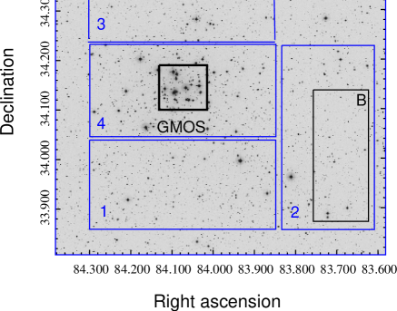
Figure 1: A digitized sky survey image around NGC 1960. The four outer rectangles (blue in the electronic version) mark the footprint of the $RI$ survey with the Isaac Newton Telescope Wide Field Camera (WFC), with CCD numbers labelled. No useful data were obtained in the north-east corner of CCD 3 because of vignetting. The central square (black in the electronic version) inside CCD 4 marks the Gemini GMOS field in which the spectroscopy was taken (see Section 4.1). The rectangle away from the cluster centre marked “B” inside CCD 2, is a “background box”, discussed in Section 5.1.

NGC 1960 ($=$ M36) is a rich, northern hemisphere (RA$=$ 05h 36m, Dec$=+$34d 08m) cluster containing about 15 objects with $V<10$, corresponding to $M\geq 4M_{\odot}$ at the distance/reddening of the cluster (see below). The first systematic studies were by Barkhatova et al. (1985) who used photoelectric photometry (from Johnson & Morgan 1953) and their own photographic $UBV$ photometry to estimate a reddening $E(B-V)=0.24$, a distance $d=1200$ pc and an age of 30 Myr determined from the main sequence turn-off. Sanner et al. (2000) present proper motions (to $V=14$) and $BV$ CCD photometry (to $V=19$), finding a clean cluster main sequence for $V<14$ and determining $E(B-V)=0.25\pm 0.02$, $d=1318\pm 120$ pc and an age of $16^{+10}_{-5}$ Myr. Sharma et al. (2006) used $UBVRI$ CCD photometry to determine $E(B-V)=0.22$, $d=1330$ pc and an age of 25 Myr. These authors also examined the radial dependence of surface density in the cluster, finding a core radius of 3.2 arcminutes and no evidence for mass segregation.

Mayne & Naylor (2008) used the Johnson and Morgan (1953) photometry and a maximum likelihood fitting technique to obtain $E(B-V)=0.20\pm 0.02$ and $d=1174^{+61}_{-42}$ pc. Bell et al. (2013) have adopted a similar maximum likelihood technique and applied it to both the high- and low-mass populations of NGC 1960, using updated atmospheres and bolometric corrections and a new method of applying reddening to stars over a wide range of colours. They used the $U-B$ versus $B-V$ diagram for the high-mass stars to derive a mean reddening $E(B-V)=0.20$, with a negligible statistical uncertainty and no evidence for differential reddening. Applying this reddening to the $V$ versus $B-V$ CMD they obtained a best fit age and intrinsic distance modulus of $26.3^{+3.2}_{-5.2}\,\rm{Myr}$ and $10.33^{+0.02}_{-0.05}$ mag ($d=1164^{+11}_{-26}$ pc). With the distance and reddening fixed at these values, Bell et al. were then able to fit lower mass cluster members in the $g$ versus $g-i$ CMD, finding an age of 20 Myr with negligible statistical error, but variations of $\sim 2$ Myr depending on which evolutionary models were adopted. The distance modulus and reddening derived by Bell et al. is used in the rest of this paper.

3 A CCD Photometric Survey

Figure 2: A colour-magnitude diagram for unflagged objects with uncertainties $<0.1$ mag in $I_{C}$ and $R_{C}-I_{C}$ seen in CCD 4 (see Fig. 1). The dashed and solid lines show theoretical 25 Myr PMS isochrones (from Baraffe et al. 1998, with a mixing length of 1.0 pressure scale heights, and from Siess, Dufour & Forestini 2000 respectively) at an intrinsic distance modulus of 10.33, and with a reddening/extinction corresponding to $E(R_{C}-I_{C})=0.143$ (see Section 2). The objects for which GMOS spectroscopy were obtained are indicated.

Table 1: The range of colours for the photometric standards observed by each CCD detector.

CCD	Colour range
1	0.340 $<R_{C}-I_{C}<$ 1.839
2	0.318 $<R_{C}-I_{C}<$ 1.750
3	0.342 $<R_{C}-I_{C}<$ 2.323
4	0.207 $<R_{C}-I_{C}<$ 2.314

Table 2: The $I_{C}$ vs $R_{C}-I_{C}$ photometric catalogue. The full table is only available in electronic form, a portion is shown here to illustrate its content. Columns list the Field and CCD number on which the star appeared (only one field was observed), a unique identifier on that CCD, Right Ascension and Declination (J2000.0), the CCD pixel coordinates at which the star was found, and then for each of $I_{C}$ and $R_{C}-I_{C}$ there is a magnitude, magnitude uncertainty and a flag (OO for a “clean”, unflagged detection – a detailed description of the flags is given by Burningham et al. [2003]).

CCD	ID	RA	Dec	x	y	$I_{C}$	$\Delta I_{C}$	flag	$R_{C}-I_{C}$	$\Delta(R_{C}-I_{C})$	flag
		(J2000.0)		(pixels)		(mag)			(mag)
1.01	449	05 35 44.081	+33 59 44.41	566.589	3309.792	9.431	0.010	SS	0.735	0.013	SS
1.02	415	05 35 4.242	+33 54 25.10	1459.969	3537.820	9.649	0.011	LS	0.887	0.014	LS
1.04	242	05 36 32.003	+34 10 47.21	665.336	1525.915	9.702	0.010	SS	0.337	0.013	SS

In order to select faint, low-mass targets for subsequent spectroscopy, a photometric survey of NGC 1960 was performed using the Wide Field Camera (WFC) at the Isaac Newton Telescope (INT) on La Palma on the night of the 28th September 2004. The WFC consists of 4 thinned EEV 2k$\times$4k CCDs (numbered 1–4) covering 0.33 arcsec/pixel on the sky. The arrangement of the 4 detectors on the sky for our observations of NGC 1960 is shown in Fig. 1. Exposures were obtained in the Sloan $r$-band (3s, 30s and 3$\times$350s) and Sloan $i$-band (2s, 20s and 3$\times$200s). The night was photometric, and so observations of standard stars from Landolt (1992) and Stetson (2000) were obtained in the Cousins $RI$ system. Table 1 shows the range in colour of standards observed for each CCD.

The data were de-biassed and flatfielded using master bias and master twilight sky flat frames. The $i$-band data were defringed using a library fringe frame. Photometry was extracted using the optimal techniques described by Naylor (1998) and Naylor et al. (2002). The sum of all three long $i$-band frames was searched to produce a catalogue of object positions, and then optimal photometry was performed at these positions in all frames, modelling the background with a skewed Gaussian distribution (see Burningham et al. 2003). By comparing measurements in the long $r$ frames we established that a one percent magnitude-independent uncertainty should be added to measurements from a single frame. This was included when measurements were combined to yield a single magnitude for each star in each filter. The optimal photometry magnitudes were corrected to that of a large aperture using a spatially dependent aperture correction (see Naylor et al. 2002).

Standard star photometry was also extracted using optimal photometry techniques and corrected to a larger aperture in the same way as the target data. The advantage of this over the more usual method of performing photometry directly in a large aperture, was that good signal-to-noise photometry was collected on many more faint standards. The only disadvantage might be that the standard star magnitudes were originally defined using a large aperture that included nearby contaminating objects. However, our reduction process flags photometry that is significantly perturbed by nearby companions and in any case many fainter standards (from Stetson 2000) were originally defined using PSF-fitting.

The observed standard star instrumental magnitudes were modelled as a function of colour and airmass to obtain extinction coefficients, zero points and colour terms. The airmass range of the standard stars is small (1.1 to 1.3) and close to the airmass of the target observations (1.1), and so the extinction was fixed at a single value. Although a single linear relationship was sufficient to represent the conversion from instrumental $i$ to $I_{C}$ as a function of $R_{C}-I_{C}$, we found we had to use two separate linear relationships to convert instrumental $r-i$ to $R_{C}-I_{C}$, with the break occuring at $R_{C}-I_{C}=1.0$ to 1.3 depending on CCD. A magnitude-independent uncertainty of 1 per cent in $R_{C}-I_{C}$ and 2 per cent in $I_{C}$ were required to obtain a reduced $\chi^{2}$ of unity in our fits. These values correspond to the combined uncertainty in the profile correction and correction to the Cousins system. They are not included in the uncertainty estimates in the final catalogues, as they should not be added when comparing stars in a similar region of the CCD (see Naylor et al. 2002). The astrometric calibration uses objects in the 2MASS point source catalogue (Cutri et al. 2003), with a RMS of 0.1 arcsec for the fit of pixel position as a function of RA and Dec.

The entire catalogue is presented as Table 2, which is available on-line, or from the Centre de Données astronomiques de Strasbourg (CDS) or from the “Cluster” Collaboration’s home page. Fig. 2 shows the $I_{C}$ vs $R_{C}-I_{C}$ colour-magnitude diagram (CMD) for all unflagged (i.e. clean, star-like, with good photometry) objects on CCD 4 with colours and magnitudes that have a signal-to-noise ratio (SNR) greater than 10. This illustrates a clear PMS at the position in the CMD appropriate for a $\sim 25$ Myr population at a distance of $1164$ pc and a reddening $E(R_{C}-I_{C})=0.143$ (corresponding to $E(B-V)=0.20$ – Taylor 1986). Isochrones are plotted in Fig. 2 from Siess, Dufour & Forestini (2000, with metallicity of 0.02) and Baraffe et al. (1998, with mixing length of 1.0 pressure scale heights), where the luminosities and temperatures were transformed to the observational plane using a fit to empirical bolometric corrections from Leggett (1992) and Leggett et al. (1996) and a colour-$T_{\rm eff}$ relationship that was tuned so that a 120 Myr isochrone gave a match to low-mass photometry in the Pleiades cluster (see Jeffries et al. 2004 for details of this procedure). The sharp magnitude cut-off in Fig. 2 is an artefact of the signal-to-noise threshold placed on the plotted points. We judge our data to be almost complete down to this cut-off, although the catalogue detection limit is about 1 magnitude fainter.

4 Gemini Spectroscopy

4.1 Target selection

Table 3: The identifiers from Table 2, positions and photometry for the Gemini targets and an integer that indicates in which slit masks the object was targeted (e.g. 12 indicates that the object was targeted in masks 1 and 2). The $RI$ photometry is in the Cousins system and comes from the survey presented here. The gri photometry are from Bell et al. (2013), except for star 1.04 3081 which is from a reduction which excludes the deepest i-band image, as a defect in this image caused the photometry to be flagged. The gri data are AB photometric magnitudes calibrated to the natural photometric system of the INT-WFC (see Bell et al. 2012).

CCD	ID	RA	Dec	$I_{C}$	$\Delta I_{C}$	$R_{C}-I_{C}$	$\Delta(R_{C}-I_{C})$	$i$	$\Delta i$	$g-i$	$\Delta(g-i)$	$r-i$	$\Delta(r-i)$	Mask(s)
		(J2000.0)		(mag)
1.04	827	5 36 28.151	34 06 56.30	16.583	0.008	0.920	0.009	17.086	0.009	2.201	0.015	0.842	0.013	1
1.04	829	5 36 27.929	34 07 01.14	16.591	0.008	0.875	0.009	17.063	0.009	2.142	0.015	0.778	0.013	3
1.04	876	5 36 07.313	34 09 41.31	16.508	0.008	0.841	0.009	16.922	0.009	1.955	0.014	0.717	0.013	1
1.04	1018	5 36 27.761	34 08 14.77	16.806	0.008	0.896	0.009	17.289	0.009	2.084	0.015	0.813	0.014	1
1.04	1025	5 36 25.696	34 09 52.78	16.878	0.008	0.889	0.009	17.360	0.009	1.972	0.015	0.800	0.014	1
1.04	1042	5 36 19.355	34 10 32.51	16.729	0.012	0.939	0.016							3
1.04	1056	5 36 14.361	34 10 40.92	16.979	0.008	1.056	0.009	17.496	0.009	2.388	0.017	0.966	0.014	2
1.04	1269	5 36 24.402	34 11 32.77	17.284	0.009	1.146	0.010	17.848	0.010	2.578	0.020	1.114	0.015	1
1.04	1291	5 36 15.712	34 10 38.80	17.181	0.009	1.234	0.010	17.736	0.010	2.560	0.019	1.158	0.015	1
1.04	1540	5 36 13.467	34 06 56.83	17.678	0.010	1.554	0.012	18.269	0.010	2.865	0.030	1.493	0.017	2
1.04	1545	5 36 13.330	34 11 27.49	17.509	0.009	1.322	0.010	18.047	0.010	2.629	0.023	1.231	0.015	3
1.04	1833	5 36 24.869	34 07 49.36	17.357	0.009	1.219	0.010	17.919	0.010	2.624	0.022	1.188	0.015	1
1.04	1859	5 36 17.460	34 10 50.76	17.863	0.010	1.542	0.013	18.371	0.010	2.875	0.044	1.423	0.020	123
1.04	1860	5 36 17.328	34 11 28.79	17.853	0.010	1.535	0.012	18.490	0.020	2.846	0.077	1.459	0.068	2
1.04	1871	5 36 13.418	34 06 36.46	18.015	0.011	1.549	0.013	18.602	0.011	2.965	0.041	1.496	0.019	23
1.04	1878	5 36 10.735	34 06 32.87	17.712	0.010	1.533	0.012	18.306	0.010	3.029	0.033	1.498	0.017	1
1.04	2160	5 36 26.501	34 11 15.02	18.132	0.011	1.544	0.014	18.770	0.011	2.793	0.042	1.480	0.020	3
1.04	2171	5 36 24.976	34 11 02.18	18.191	0.011	1.625	0.015	18.999	0.024	3.504	0.297	1.539	0.118	123
1.04	2173	5 36 24.429	34 09 00.62	18.334	0.012	1.625	0.016	18.952	0.011	3.080	0.059	1.621	0.023	123
1.04	2188	5 36 19.966	34 07 46.22	18.179	0.011	1.581	0.015	18.822	0.011	2.899	0.051	1.514	0.022	23
1.04	2214	5 36 13.449	34 06 31.98	18.213	0.012	1.587	0.015	18.856	0.011	3.020	0.048	1.568	0.021	23
1.04	2249	5 36 05.655	34 08 13.25	18.270	0.012	1.747	0.017	18.928	0.011	3.253	0.069	1.677	0.024	23
1.04	2663	5 36 16.260	34 10 12.99	18.412	0.013	1.699	0.018	19.054	0.012	3.076	0.063	1.687	0.025	123
1.04	2672	5 36 13.557	34 11 13.38	18.658	0.014	1.733	0.021	19.305	0.022	3.098	0.145	1.758	0.103	12
1.04	2696	5 36 09.583	34 09 43.17	18.584	0.014	1.695	0.019	19.240	0.012	3.149	0.080	1.703	0.028	23
1.04	2703	5 36 07.694	34 07 10.82	18.490	0.013	1.694	0.018	19.097	0.012	3.222	0.072	1.629	0.024	123
1.04	3028	5 36 29.903	34 09 18.92	19.060	0.019	1.919	0.032	19.754	0.014	3.685	0.200	1.921	0.047	123
1.04	3073	5 36 20.090	34 08 48.03	18.785	0.016	1.801	0.025	19.460	0.013	3.152	0.095	1.83	0.036	123
1.04	3080	5 36 18.218	34 08 28.28	18.795	0.016	1.896	0.026	19.442	0.013	3.533	0.143	1.891	0.036	123
1.04	3081	5 36 18.210	34 08 03.34	18.711	0.021	1.711	0.077	19.380	0.015	3.210	0.146	1.862	0.051	123
1.04	3150	5 36 05.662	34 09 29.78	18.843	0.016	1.827	0.025	19.532	0.013	3.238	0.113	1.875	0.039	123
1.04	3590	5 36 18.307	34 10 24.67	19.107	0.019	1.864	0.033	19.779	0.015	3.786	0.228	1.973	0.053	123
1.04	3596	5 36 17.363	34 10 02.63	19.185	0.020	1.903	0.036	19.895	0.015	3.276	0.153	1.756	0.046	123
1.04	3612	5 36 13.674	34 06 45.40	19.152	0.021	1.914	0.037	19.822	0.015	3.536	0.190	1.796	0.046	123
1.04	4165	5 36 10.731	34 07 25.67	19.469	0.025	1.992	0.049	20.213	0.018	3.682	0.275	2.044	0.074	123

The Gemini Multi-Object Spectrograph (GMOS) was used at the Gemini North telescope to observe 35 candidate low-mass members of NGC 1960 with $16.5<I_{C}<19.5$. This corresponds to an approximate mass range of $0.15<M/M_{\odot}<0.85$ according to the models of Baraffe et al. (1998). Stars, with unflagged photometry, were targeted based on their location in the $I_{C},R_{C}-I_{C}$ CMD, following the location of the obvious PMS (see Fig. 2). Targets were included in three separate slit mask designs covering the $5.5\times 5.5$ arcmin² GMOS field of view, centered at a single sky position (see Fig. 1). The faintest targets were observed through all three masks, but to cover a larger number of targets, the brighter candidates were observed through just one or two of the masks. Table 3 gives the coordinates and photometry of the targets and lists which masks they were observed in. In addition we list photometry in the $gri_{\rm WFC}$ system from the photometric survey subsequently performed and detailed in Bell et al. (2013). This latter survey has slightly poorer precision (and one target did not have good photometry), but serves as a useful check on systematic photometric calibration uncertainties. Good 2MASS photometry was unavailable for most of the faint targets in the sample, including those around the LDB (see Section 5.2), so was not considered.

4.2 Observations and Data Reduction

Table 4: Gemini GMOS observation log giving the date and time (UT) at the start of each sequence of 3 exposures, the mask number, the number of targets in each mask, the exposure times and the average seeing.

Date/Time	Slit Mask	$N_{\rm targ}$	Exposure	Seeing
(UT)			(s)	(arcsec)
01/11/2005 13:48	Mask 1	26	$3\times 1800$	0.6
06/11/2005 13:05	Mask 3	23	$3\times 1800$	0.6
27/11/2005 08:26	Mask 2	23	$3\times 1800$	0.8
28/11/2005 07:38	Mask 2	23	$3\times 1800$	0.7
02/12/2005 12:34	Mask 1	26	$3\times 1800$	0.6
03/12/2005 12:38	Mask 1	26	$3\times 1800$	0.5

Figure 3: Example spectra from our target list, covering the full range of spectral type and signal-to-noise ratio. Spectra have been subject to relative flux calibration, telluric correction and have been normalised to a continuum point near H$\alpha$. The inserts on each plot show normalised spectra in the regions of the H$\alpha$ and Li i 6708Å lines. Plots are ordered according to spectral type (see Section 4.3.1) and labelled according to the target ID in Table 3.

Each mask setup was observed from one to three times. The observations were taken in queue mode during November and December 2005 (see Table 4). On each occasion that a mask was observed, we obtained $3\times 1800$ s exposures bracketed by observations of a CuAr lamp for wavelength calibration and a quartz lamp for flat-fielding and slit location. The net result was that all of the targets received at least 90 minutes of exposure, whilst the faintest targets, present in all three masks, were observed for a total of 9 hours.

We used slits of width 0.5 arcsec and with lengths of 8–10 arcsecs. The R831 grating was used with a long-pass OG515 filter to block second order contamination. The resolving power was 4400 and simultaneous sky subtraction of the spectra was possible. The spectra covered $\sim 2000$Å, with a central wavelength of 6200Å– 7200Å depending on slit location within the field of view.

The spectra were recorded on three $2048\times 4068$ EEV chips leading to two $\simeq 16$Å gaps in the coverage. The CCD pixels were binned $2\times 2$ before readout, corresponding to $\sim 0.67$Å per binned pixel in the dispersion direction and 0.14 arcsec per binned pixel in the spatial direction. Conditions were clear with seeing of 0.5–0.8 arcsec (FWHM measured from the spectra).

The data were reduced using version 1.8.1 of the GMOS data reduction tasks running with version 2.12.2a of the Image Reduction and Analysis Facility (iraf). The data were bias subtracted, mosaiced and flat-fielded. A two-dimensional wavelength calibration solution was provided by the arc spectra and then the target spectra were sky-subtracted and extracted using 2 arcsec apertures. The three individual spectra for each target were combined using a rejection scheme which removed obvious cosmic rays. The instrumental wavelength response was removed from the combined spectra using observations of a white dwarf standard to provide a relative flux calibration. The same calibration spectrum was used to construct a telluric correction spectrum. A scaled version of this was divided into the target spectra, tuned to minimise the RMS in regions dominated by telluric features. The combined spectra were corrected to the heliocentric reference frame and where multiple observations of a target were obtained on more than one occasion through the same mask or through different masks, these were tested for radial velocity variations (see below) before combining into a single summed spectrum for each target.

The SNR of each summed spectrum was estimated empirically from the RMS deviations of straight line fits to segments of “pseudo-continuum” close to the Li I 6708Å features (see below). As small unresolved spectral features are expected to be part of these pseudo-continuum regions, these SNR estimates, which range from $\sim 20$–30 in the faintest targets to $>100$ in the brightest, should be lower limits. Examples of the reduced spectra are shown in Fig. 3. All the reduced spectra are available in “fits” format from the “Cluster” Collaboration’s home page (see footnote 1).

4.3 Analysis

Each spectrum was analysed to yield a spectral type, equivalent widths of the Li I 6708Å and H$\alpha$ lines and a heliocentric RV. Each of these analyses is described below. The results are given in Table 5.

Table 5: Results from the spectroscopic analyses. Columns list the identifiers from Table 2, photometry, the signal-to-noise ratio of the summed spectra, the TiO index, derived spectral type (on a numerical scale where $-2=$K5, $-1=$K7, $0=$M0, $1=$M1 etc.), the H$\alpha$ equivalent width (negative $=$ absorption), the radial velocity, dispersion in the radial velocity from multiple measurements and number of spectra/radial velocity measurements, the lithium equivalent width (or 3-sigma upper limit) and its uncertainty.

CCD	ID	$I_{C}$	$R_{C}-I_{C}$	SNR	TiO	SpT	H$\alpha$ EW	RV	$\sigma$RV	nRV	Li EW
		(mag)					(Å)	(km s-1)			(Å)
1.04	827	16.583	0.920	92	1.16	-0.6	2.0	-7.2	2.5	3	$0.53\pm 0.02$
1.04	829	16.591	0.875	61	1.11	-1.0	0.2	-9.4		1	$0.31\pm 0.03$
1.04	876	16.508	0.841	133	1.09	-1.2	1.7	5.9	2.1	3	$0.56\pm 0.01$
1.04	1018	16.806	0.896	119	1.01	-1.9	-1.5	-2.0	2.0	3	$<0.04$
1.04	1025	16.878	0.889	218	1.01	-2.0	-2.8	-52.6	4.2	3	$<0.03$
1.04	1042	16.729	0.939	64	1.14	-0.8	0.7	-1.3		1	$0.40\pm 0.03$
1.04	1056	16.979	1.056	86	1.23	-0.1	2.4	-6.8	1.7	2	$0.34\pm 0.02$
1.04	1269	17.284	1.146	124	1.32	0.6	1.5	-7.1	1.7	3	$0.12\pm 0.01$
1.04	1291	17.181	1.234	77	1.46	1.5	5.0	-3.0	2.7	3	$0.47\pm 0.02$
1.04	1540	17.678	1.554	79	1.80	3.1	6.1	-1.7	3.0	2	$<0.06$
1.04	1545	17.509	1.322	29	1.51	1.7	2.9	-5.1		1	$<0.17$
1.04	1833	17.357	1.219	153	1.43	1.3	3.5	-7.8	1.9	3	$0.15\pm 0.01$
1.04	1859	17.863	1.542	91	1.74	2.9	5.0	-6.8	4.0	6	$<0.05$
1.04	1860	17.853	1.535	63	1.83	3.2	5.2	-6.9	1.2	2	$<0.08$
1.04	1871	18.015	1.549	35	1.75	2.9	3.8	-5.6	0.6	3	$<0.14$
1.04	1878	17.712	1.533	100	1.63	2.4	5.5	-4.0	4.4	3	$<0.05$
1.04	2160	18.132	1.544	71	1.92	3.6	-0.3	-9.1		1	$<0.07$
1.04	2171	18.191	1.625	93	1.91	3.5	5.8	-5.1	2.6	6	$<0.05$
1.04	2173	18.334	1.625	81	1.95	3.6	4.6	-5.3	8.4	6	$<0.06$
1.04	2188	18.179	1.581	37	1.88	3.4	3.3	-7.7	0.6	3	$<0.13$
1.04	2214	18.213	1.587	50	1.89	3.4	3.9	-3.7	2.3	3	$<0.10$
1.04	2249	18.270	1.747	41	2.10	4.1	4.6	-1.2	1.1	3	$<0.12$
1.04	2663	18.412	1.699	46	2.06	4.0	6.6	-1.0	1.7	6	$<0.10$
1.04	2672	18.658	1.733	50	2.07	4.0	6.3	-0.4	1.9	5	$<0.10$
1.04	2696	18.584	1.695	24	2.02	3.9	5.0	-2.1	1.1	3	–
1.04	2703	18.490	1.694	51	1.95	3.6	6.4	-9.7	2.1	6	$<0.10$
1.04	3028	19.060	1.919	40	2.29	4.5	5.1	-1.5	2.4	6	$<0.12$
1.04	3073	18.785	1.801	45	2.22	4.4	6.7	-0.1	2.3	6	$<0.11$
1.04	3080	18.795	1.896	34	2.43	4.8	6.9	-8.8	5.0	6	$0.69\pm 0.05$
1.04	3081	18.711	1.711	33	2.24	4.4	4.7	-4.8	3.1	6	$0.17\pm 0.05$
1.04	3150	18.843	1.827	52	2.27	4.5	6.2	-8.3	2.2	6	$<0.09$
1.04	3590	19.107	1.864	31	2.31	4.6	5.8	-2.3	3.8	6	$<0.15$
1.04	3596	19.185	1.903	29	2.33	4.6	6.4	-5.3	0.5	6	$0.62\pm 0.05$
1.04	3612	19.152	1.914	33	2.13	4.2	5.0	4.5	0.7	6	$<0.15$
1.04	4165	19.469	1.992	26	2.28	4.5	4.1	1.6	6.6	6	$<0.19$

4.3.1 Spectral Types

Figure 4: Spectral types deduced from the TiO(7140Å) index as a function of $R_{C}-I_{C}$. Three stars with H alpha absorption lines (and presumably non-members – Section 5.1) are indicated. Also shown are results from the spectra of standard stars where $R_{C}-I_{C}$ is available (see text).

Table 6: The relationship between TiO(7140Å) index and spectral type calibrated from standards in Montes et al. (1997) and Barrado y Navascués et al. (1999).

Index	Spectral Type
0.99	K5
1.13	K7
1.26	M0
1.40	M1
1.53	M2
1.74	M3
2.08	M4
2.61	M5
3.38	M6

Spectral types were estimated from the strength of the TiO(7140Å) narrow band spectral index (e.g. Briceño et al. 1998; Oliveira et al. 2003). This index is temperature sensitive and calibrated using the spectral types of well known late-K and M-type field dwarfs taken from spectra in Montes et al. (1997) and Barrado y Navascués et al. (1999). We constructed a polynomial relationship between spectral type and the TiO(7140Å) index that was used to estimate the spectral type of our targets, based on a numerical scheme where M0–M6$=$0–6, K5 $=-2$ and K7 $=-1$. Table 6 gives the adopted relationship between the TiO(7140Å) index and spectral type. The scatter around the polynomial indicates that these spectral types are good to $\pm$ 0.3 subclasses for stars of type M1 and later, but about twice this for earlier spectral types where the molecular bands are weak.

A plot of spectral type, from the TiO(7140Å) index, versus $R_{C}-I_{C}$ colour reveals a smooth relationship (see Fig. 4) with little scatter. The most likely contaminants among our candidate members are foreground M-type field dwarfs with similar spectral types but lower luminosities or background K-giants. It is possible that these could have different reddening that might make them stand out in this diagram, but no objects exhibit a significant deviation. A comparison of the positions of some of the standard stars on this plot ($R_{C}-I_{C}$ colours where available are from Leggett 1992) reveals an average redward offset of $\simeq 0.1$ mag in the $R_{C}-I_{C}$ values of our targets at a given spectral type. We expect cluster members to have suffered a reddening $E(R_{C}-I_{C})\simeq 0.14$ mag. Whilst this comparison provides some evidence that the photometric calibration for these red stars is reasonable, we have to temper this conclusion with the possibility that the relationship between colour and spectral type could alter for PMS stars with lower surface gravity.

4.3.2 H-alpha measurements

Figure 5: Equivalent width (EW) of the H$\alpha$ line versus spectral types. A typical error bar is indicated. The majority of stars show H$\alpha$ emission commensurate with chromospheric activity from young stars. None of the targets has H$\alpha$ emission characteristic of accretion: the solid line shows the minimum EW expected from accretion activity (defined by Barrado y Navascués & Martín 2003). Three targets have H$\alpha$ absorption and are unlikely to be cluster members (Section 5.1).

H$\alpha$ equivalent widths (EWs) were measured by direct integration above (or below) a pseudo-continuum. The main uncertainty here is the definition of the pseudo-continuum as a function of spectral type and probably results in uncertainties of order 0.2Å, even for the bright targets.

H$\alpha$ emission is ubiquitous from young stars. It arises either as a consequence of chromospheric activity or is generated by accretion activity in very young objects (e.g. Muzerolle, Calvet & Hartmann 1998). It is unlikely that accretion persists in stars much beyond 10 Myr (e.g. Jeffries et al. 2007; Fedele et al. 2010). The H$\alpha$ emission from accreting “classical” T-Tauri stars (CTTS) is systematically stronger and broader than the weak line T-Tauri stars (WTTS) where the emission is predominantly chromospheric.

Fig. 5 shows the H$\alpha$ EW as a function of spectral type for our targets. None has H$\alpha$ emission strong enough to indicate accretion according to criteria defined by White & Basri (2003) and Barrado y Navascués & Martín (2003), but the majority have emission characteristic of the chromospheric activity expected for low-mass stars with an age of $\simeq 20$–$30$ Myr (e.g. Stauffer et al. 1997). Three stars have H$\alpha$ absorption lines and are unlikely to be cluster members (see Section 5.1).

4.3.3 Radial Velocities

Our observations of each target were split into 1–6 epochs, depending on in which masks the target featured. This gave the opportunity to check for binarity, or at least binaries with orbital periods shorter than a few months, by looking for RV variations.

Relative RVs were determined using the iraf procedure fxcor to cross-correlate the first spectrum in a sequence of target exposures with the rest, yielding between 0 and 5 RV difference measurements. All spectra were heliocentrically corrected before correlation. For the earlier type stars in our sample we found that the strongest cross-correlation functions were obtained in the wavelength range 6000–6500Å, though this range was truncated, at the blue end, at longer wavelengths for some targets where the spectrum fell off the CCD image. Similarly we found that the wavelength range 6600-7000Å gave the best correlations for the cooler targets. In practice, the division between warmer and cooler stars was not made absolute and we took an average of the two measurements for stars with spectral types between M2.0 and M3.5. Statistical uncertainties in each RV should be of order $\sim 100$/SNR km s^-1, but the dispersions for each target are larger than this. A probable cause is small slit mis-centering errors of order a few hundredths of an arcsecond, exacerbated by the good seeing compared to the slit width. In any case, the measured dispersions of a few km/s are a better estimate of the true uncertainties.

No measurements of RV standards were taken as part of our observing program, but heliocentric RVs were estimated by cross-correlating against a synthetic spectral library in the same wavelength ranges discussed above (generated from the Phoenix models by Brott & Hauschildt 2005). write in a synthetic way For the warmer stars we used the synthetic template of a solar metallicity star at 4000 K and with $\log g=4.5$; for the cooler stars we chose a synthetic template with solar metallicity, 3500 K and $\log g=4.0$. Again, results were averaged in the overlap region.

Table 5 gives our estimate of the heliocentric RV (the mean of results from each spectrum) and a standard deviation where multiple relative RV measurements are available. Given the likely uncertainties in each RV measurement, there is no evidence, other than perhaps for target 1.04_2173, that any of the targets have RVs that vary by more than a few km s^-1 on timescales of a month or less.

4.3.4 Lithium measurements

Figure 6: Equivalent width (EW) of the Li i 6708Å feature versus spectral type. Triangles indicate 3-sigma upper limits. The loci represent lines of constant Li abundance (A(Li) = 12 + $\log N$(Li)/$\log N$(H)) calculated from the curves of growth described by Jeffries et al. (2003) and the relationship between spectral type and temperature presented by Kenyon & Hartmann (1995).

The Li I 6708Å resonance feature should be strong in cool young stars with undepleted Li – an EW of 0.3Å to 0.6Å is predicted by curves of growth (e.g. Zapatero-Osorio et al. 2002; Jeffries et al. 2003). Theory suggests (e.g. Baraffe et al. 1998) that in a population with age $\sim 20$ Myr, the Li EW should grow towards late K-type as the line strengthens for a given abundance. Li-depletion in early- to mid-M dwarfs should result in an undetectable Li line, and then below an age-dependent luminosity, objects should have retained all their original Li and the line EW should return sharply to $\sim 0.6$Å. Insets in Fig. 3 show the Li region in a number of our targets.

Where it appeared, the EW of the Li I 6708Å feature was estimated by direct integration below a pseudo-continuum derived from fitting small regions either side of the Li line, excluding regions beyond 6712Å which contain a strong Ca line and which are noisy due to the subtraction of a strong S ii sky line. Uncertainties in the EW were estimated using the formula $\Delta{\rm EW}=1.6\sqrt{fp}/{\rm SNR}$ (Cayrel 1988), where $f$ is the FWHM ($=1.5$Å) of the unresolved line and $p$ is the pixel size ($=0.67$Å). In many cases there was no obvious Li feature to measure, in which case a $3\sigma$ ($=3\,\Delta{\rm EW}$) upper limit is quoted. In one case the Li feature fell in a gap between the detectors and no EW could be measured. Li EWs are plotted as a function of spectral type in Fig. 6. According to the curves of growth described by Jeffries et al. (2003), the measured EWs imply Li abundances from A(Li)$\simeq 3.3$ (where A(Li) = 12 + $\log N$(Li)/$\log N$(H)), corresponding to the undepleted meteoritic value (Anders & Grevesse 1989), to A(Li)$\ll 1.0$.

5 The Lithium Depletion Boundary

5.1 Cluster membership and sample contamination

Determining the LDB requires a clean sample of genuine cluster members. Several lines of evidence suggest that the vast majority of the objects targeted for spectroscopy are members of NGC 1960.

5.1.1 Photometric selection

An upper limit to the contamination of the spectroscopic sample is estimated by comparing the spatial density of objects inside the photometric selection box (in the $I_{C}$ versus $R_{C}-I_{C}$ CMD) close to the cluster centre, where the targets were selected, with the spatial density far from the cluster centre. It is an upper limit because we can not be sure that very low-mass cluster members are confined only to the central region. Sharma et al. (2006) fitted a King model to brighter stars ($V<18$) in NGC 1960, finding a core radius of only 3.2 arcminutes. If the lower mass stars follow the same profile, then their spatial density should decrease by a factor of 10 only $\sim 10$ arcminutes from the cluster centre. This analysis used a “background box” of size 104 square arcminutes about 10 arcminutes from the cluster centre (see Fig. 1). Using the same criteria used to select Gemini targets, there are 41 cluster candidates in this box, 27 with $0.8<R_{C}-I_{C}\leq 1.4$ and 14 with $1.4<R_{C}-I_{C}<2.0$. This compares with the GMOS field, with an effective area of 30 square arcminutes, that contains 37 and 97 candidates in the same colour ranges, of which we spectroscopically observed 11 and 24 respectively. If we assume the background box contains only contaminants and that their density is constant across our survey, we expect 2.3 objects in our spectroscopic sample with $0.8<R_{C}-I_{C}\leq 1.4$ to be non-members and a further 1.0 non-member with $1.4<R_{C}-I_{C}<2.0$.

5.1.2 Lithium

Eight of our targets have clear detections of the Li feature with EW $>0.3$Å. Comparisons with Li-depletion patterns in open clusters of known age (e.g. see Fig. 10 of Jeffries et al. 2003 and references therein) place empirical age constraints on these stars. Li EWs of $>0.3$Å are not seen in stars cooler than spectral type K5 in the Pleiades or Alpha Per clusters with ages of 120 Myr and 90 Myr respectively (excepting the very low luminosity M6$+$ stars beyond the LDB, where Li remains unburned). Nor can strong Li lines be seen in M dwarfs of the 35–55 Myr open clusters NGC 2547, IC 2391 and IC 2602 (again, excepting M4.5$+$ dwarfs beyond the LDB). Thus objects with EW[Li] $>0.3$Å are probably younger than 100 Myr, and younger than 50 Myr if they have spectral type M0–M5. These Li-rich objects are very likely to be members of NGC 1960 as the chances of a field star being younger than 100 Myr is of order 1 per cent. However a lack of Li cannot exclude candidates because we are observing stars that are cool enough that even at an age of 20 Myr we might expect all their Li to have been depleted, especially at spectral types M2–M4.

5.1.3 Chromospheric emission

H$\alpha$ measurements are a powerful way of excluding non-members. For instance in the Pleiades, at an age of 120 Myr, all late K- and M-dwarf members show chromospheric H$\alpha$ emission (Stauffer et al. 1997). However, the H$\alpha$ magnetic activity lifetimes of M-dwarfs range from a few hundred Myr in early M-dwarfs to almost 5 Gyr for M5 dwarfs (West et al. 2008), so there is a significant probability that contaminating foreground field M-dwarfs would still show H$\alpha$ emission. Therefore, the 3 objects in our sample that have H$\alpha$ absorption are either older foreground field dwarfs or background giants, but the H$\alpha$ emission we see in all other targets is a necessary, but not sufficient, condition for membership.

5.1.4 Radial velocities

We expect cluster members to have similar RVs, with a dispersion of a few km s^-1. Objects with RVs outside this range are either non-members or possibly cluster members in binary systems. Only one object (ID 1.04_1025) has an RV clearly discrepant from the bulk of objects. This target also has H$\alpha$ absorption, so is not a cluster member in any case. None of the objects, except perhaps $1.04\_2173$, show evidence for any RV variability.

The unweighted mean heliocentric RV of the 8 objects with EW(Li)$>0.3$Åis $-5.1\pm 1.5$ km s^-1, with a standard deviation of 4.2 km s^-1. If we take the whole sample, but exclude the three objects with H$\alpha$ absorption, the other 32 targets have an unweighted mean heliocentric RV of $-4.0\pm 0.7$ km s^-1, a standard deviation of 3.8 km s^-1, and all have RVs within 3 standard deviations of this mean. It is therefore impossible to exclude further objects on the basis of RV with any confidence and the RVs support the idea that the majority of targets share a similar RV.

In summary 3 targets (IDs 1.04_1018, 1.04_1025, 1.04_2160) are excluded as non-members. The rest have H$\alpha$ emission, RVs, spectral types and colours consistent with cluster membership. Those with Li in their atmospheres are probably younger than 100 Myr and almost certain cluster members. The level of sample contamination is as expected from the photometric selection criteria.

5.2 Locating the lithium depletion boundary

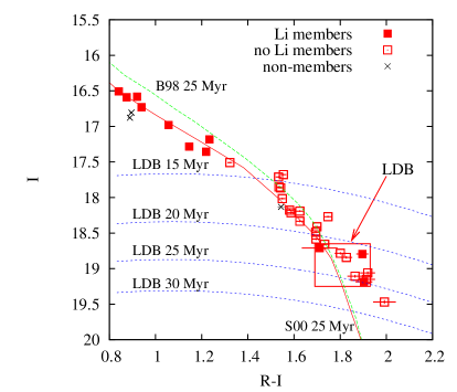
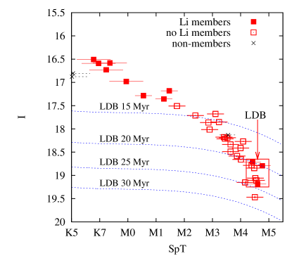
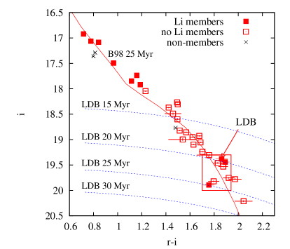
Figure 7: Colour-magnitude and spectral type-magnitude diagrams indicating which objects have detected lithium and the likely location of the lithium depletion boundary. The dashed lines in each diagram are the predicted loci of 99 per cent Li depletion according to the models of Chabrier & Baraffe (1997), using empirical bolometric corrections, reddening and extinction corresponding to $E(B-V)=0.20$ and a distance modulus of 10.33 mag (see Section 5.3). The top panel also shows 25 Myr isochrones calculated (as described in Section 3) from the interior models of Baraffe et al. (1998) and Siess et al. (2000). The bottom panel shows an equivalent isochrone calculated by Bell et al. (2013) from the Baraffe et al. models.

Fig. 6 shows that no stars have detected Li between spectral types of M2 and M4 ($3580>T_{\rm eff}>3370$ K – Kenyon & Hartmann 1995). According to theoretical models (e.g. D’Antona & Mazzitelli 1997; Chabrier & Baraffe 1997; Siess et al. 2000), at cooler temperatures the core temperatures of PMS stars remain too cool to burn Li, with an abrupt transition occurring in Li abundance between entirely depleted Li on the warm side of the boundary and undepleted Li on the cool side. This does appear to be the case in our data (see Fig. 6). The transition occurs at a spectral type of $\simeq$M4.5, with the two coolest objects (according to their spectral types, though not according to their colours) showing undepleted Li levels.

In principle, the sharp transition in Fig. 6 can be used to estimate the cluster age. In practice, the $T_{\rm eff}$ or spectral type of the LDB is not the best age indicator. As explained in Jeffries (2006), there are significant uncertainties (of order 150 K) in converting a spectral type or colour into $T_{\rm eff}$, and different evolutionary models, using different atmosphere prescriptions, differ by a similar amount in the $T_{\rm eff}$ predicted for the LDB at a given age. The relatively shallow relationship between $T_{\rm eff}$ at the LDB and age means that any small temperature uncertainty translates into a large age uncertainty. For example, an LDB at $3300\pm 150$ K, corresponding to a spectral type of M4.5, leads to an LDB age estimate of $31\pm 20$ Myr via the models of Chabrier & Baraffe (1997). As we show below, for NGC 1960 where the distance is reasonably well-determined, the LDB age is much more precisely estimated using the luminosity or absolute magnitude of the LDB. Different evolutionary models also predict very similar LDB luminosities at ages between 15 Myr and 150 Myr and relationships between bolometric correction and colour are uncertain by $<0.1$ mag, which turns out to have a negligible effect on age estimates (Jeffries & Naylor 2001).

Figure 7 shows the CMDs and spectral-type versus magnitude diagrams for our targets, indicating those with and without detected Li and those that are non-members. In each diagram an estimate is made of the colour (or spectral type) and magnitude range that marks the LDB transition between stars that have depleted more than 99 per cent of their initial Li, and those below that have retained Li. There are difficulties in chosing this location. (i) It is possible that some non-members (without Li) still lurk among the low-mass stars, although this seems unlikely to be more than 1-2 objects given the discussion in Section 5.1. (ii) Although close binarity is unlikely in any of our targets, at the distance of NGC 1960, even wide binaries with separations of several hundred au would remain unresolved. The binary frequency among these low-mass objects is expected to be of order 30 per cent. Binarity could increase the apparent luminosity of a star at a fixed colour or spectral type (for an equal mass binary) by 0.75 mag. Thus stars with Li could appear up to 0.75 mag above the LDB. (iii) There are uncertainties in the photometry and spectral types (shown in the plots) and young, low-mass stars can show time-variable colours and magnitudes at levels of $\sim 0.1$ mag.

Of the three low-luminosity stars where Li has been detected, the star 1.04_3080 shows some evidence of binarity, being $\sim 0.3$ mag brighter than the average object at the same colour/spectral type in all three diagrams. The star 1.04_3081 is the brightest of the three, but its EW(Li) of $0.17\pm 0.05$Å suggests it may already have depleted $\sim 99$ per cent of its initial Li content. We therefore define the LDB to lie in the boxes shown in Fig. 7, which allow a generous level of uncertainty.

5.3 Ages from the LDB

The central points of the LDB boxes in Fig. 7 are translated into ages as follows. The evolutionary models of Chabrier & Baraffe (1997) are interpolated to find a relationship between the luminosity and age at which the initial Li content is depleted by 99 per cent. These luminosities are converted into absolute magnitudes at any given colour or spectral type using empirical bolometric corrections. For the $I_{C}$ versus $R_{C}-I_{C}$ diagram we use a relationship between bolometric correction and colour obtained by fitting a quadratic to data found in Leggett (1992) and Leggett et al. (1996)

$${\rm BC}_{I}=0.174+0.882(R_{C}-I_{C})-0.4753(R_{C}-I_{C})^{2}\,,$$ (1)

valid for $1.0<R_{C}-I_{C}<2.4$, with a scatter of 0.06 mag. For the $I_{C}$ versus spectral type diagram we use a relationship between BC_I and spectral type derived from data given in Bessell (1991)

$${\rm BC}_{I} = 0.595-0.0108\,{\rm SpT}-0.00222\,{\rm SpT}^{2}$$ (2)

$$-0.00342\,{\rm SpT}^{3},$$

where SpT is the numerical spectral type given in Table 5 and the relation is calibrated between types K7 and M6 with a scatter of 0.02 mag. For the $i$ versus $r-i$ diagram we use a polynomial fit to gravity- and temperature-dependent empirical bolometric corrections calculated by Bell et al. (2012, 2013):

$${\rm BC}_{i} = -0.068-0.09797(r-i)+0.02586(r-i)^{2}$$ (3)

$$-0.064736(r-i)^{3}\,,$$

which is valid for $0.8<r-i<2.5$ with a scatter of 0.04 mag.

The relationship between luminosity at the LDB and age combined with the bolometric corrections, define constant luminosity isochrones in the colour-magnitude or spectral type-magnitude diagrams. These isochrones are compared with the observed data in Fig. 7 by making the appropriate corrections for distance modulus (assumed to be $10.33$) and reddening (either $E(R_{C}-I_{C})=0.143$ or $E(r-i)=0.13$) and extinction (either $A_{I}=0.37$ or $A_{i}=0.38$). These isochrones can be interpolated to obtain the LDB age corresponding to any location in the diagrams. This way of displaying the data and models has the advantage of explicitly showing the influence of any particular choice of LDB location or uncertainties in distance and reddening on the derived age.

Observational uncertainties in the LDB age are derived by perturbing the LDB location by the uncertainties implied by the boxes in Fig. 7, by uncertainties in the distance modulus, reddening and extinction and we also conservatively assume that the magnitudes and colours suffer from systematic uncertainties of 0.1 mag at these red colours and that the spectral type scale may have systematic uncertainties of half a subclass. All these perturbations are combined in quadrature to give uncertainties in the bolometric magnitude at the LDB and consequent uncertainties in the LDB age. This total uncertainty is dominated by the size of the boxes in Fig. 7. The uncertainties due to distance, extinction, reddening and photometric calibration are small in comparison. The relevant data and results are presented in Table 7.

Some idea of additional systematic errors can be gained from comparing the bolometric magnitudes and ages deduced from the three separate diagrams. There are differences of order 0.15 mag and 1.5 Myr respectively, which are smaller than the observational uncertainties. Additional model dependencies are checked by: (i) Calculating the LDB age assuming that the LDB location refers to the point at which Li is depleted by 90 or 99.9 per cent rather than 99 per cent. This conservatively allows for an order of magnitude uncertainty in the Li abundance predicted from a Li EW, but only changes the ages by $\pm 1.5$ Myr, due to the rapid depletion of Li once Li-burning is initiated. (ii) Calculating the LDB ages using the models of D’Antona & Mazzitelli (1997), Siess et al. (2000, with metallicity 0.02 or 0.01) and Burke et al. (2004). These results are also given in Table 7 for each of the three diagrams in Fig. 7. The use of alternative models changes the derived age by $\pm 2$ Myr, illustrating how insensitive the LDB age is to choice of atmosphere, convection treatment or even factors of two in metallicity.

Considering all the results, we give a final estimate for the LDB age of NGC 1960 as $22\pm 3.5$ Myr, where the observational uncertainty is primarily associated with locating the LDB in sparse data. There is then a further $\pm 2$ Myr associated with choice of evolutionary model and bolometric corrections, leading to a final result of $22\pm 4$ Myr. It is important to separate out these two uncertainty contributions, since the former could be almost eliminated by locating the LDB with more precision.

Table 7: The locations of the lithium depletion boundary in colour-magnitiude or spectral type-magnitude diagrams. These locations are translated into a bolometric magnitude using an intrinsic distance modulus of 10.33 along with extinctions, reddening and bolometric corrections as described in Section 5.3. These bolometric magnitudes imply masses and LDB ages (from the models of Chabrier & Baraffe 1997) as shown and LDB ages are also calculated for for a variety of other evolutionary models.

	$I_{C}$ vs $R_{C}-I_{C}$	$I_{C}$ vs SpT	$i$ vs $r-i$
LDB location	$I_{C}=18.95\pm 0.30$	$I_{C}=18.95\pm 0.30$	$i=19.65\pm 0.35$
	$R_{C}-I_{C}=1.81\pm 0.12$	SpT $=$ M4.6$\pm 0.4$	$r-i=1.82\pm 0.12$
$M_{\rm bol}$	$8.57\pm 0.33$	$8.41\pm 0.35$	$8.47\pm 0.37$
Mass ($M_{\odot}$)	$0.23\pm 0.04$	$0.25\pm 0.04$	$0.24\pm 0.04$
Ages (Myr)
Chabrier & Baraffe 1997	$23.2^{+3.5}_{-3.1}$	$21.6^{+3.5}_{-3.0}$	$22.2^{+3.8}_{-3.3}$
D’Antona & Mazzitelli 1997	$19.8^{+3.8}_{-3.1}$	$18.3^{+3.6}_{3.0}$	$18.7^{+4.1}_{-3.3}$
Siess et al. 2000 (Z=0.02)	$23.1^{+3.8}_{-3.4}$	$21.5^{+3.8}_{-3.5}$	$22.0^{+4.1}_{-3.8}$
Siess et al. 2000 (Z=0.01)	$21.7^{+3.8}_{-3.3}$	$20.1^{+3.7}_{-3.2}$	$20.6^{+4.1}_{-3.5}$
Burke et al. 2004	$21.3^{+3.7}_{-3.1}$	$19.8^{+3.5}_{-2.0}$	$20.3^{+4.0}_{-3.2}$

6 Discussion

6.1 The sharpness of the LDB

NGC 1960 is the eighth cluster with an LDB age and also the youngest. The data in Fig. 7 allow a reasonable estimate of the LDB location, but in each case there is at least one star without Li fainter than the adopted LDB and other Li-poor stars that share similar locations to the two Li-rich (approximately undepleted) low-mass stars. This might be explained by a combination of binarity, photometric uncertainties and contamination by Li-poor non-members (see Section 5.2). However, Fig. 7 shows that it would only take an age spread of $\sim 5$ Myr within the NGC 1960 cluster to effectively blur the LDB location and lead to mixing between the Li-poor and Li-rich populations. Age spreads of this size are controversial, but may explain the Hertzsprung-Russell diagrams of very young clusters (e.g. Palla & Stahler 2000, but see counter arguments in Hartmann 2001) and the spread of Li depletion amongst low-mass stars ($M\simeq 0.1$ – $0.3\,M_{\odot}$) in some star forming regions (Palla et al. 2007; Sacco et al. 2007). The LDB of NGC 2547, which is better defined than that of NGC 1960 by a larger sample of Li-rich and Li-poor members, also shows some evidence for this blurring (Jeffries & Oliveira 2005). However, because NGC 2547 is older ($35\pm 3$ Myr) than NGC 1960, the LDB isochrones are closer together and the effects of any genuine age spread are diminished with respect to those mimicked by binarity, photometry errors and variability. NGC 1960 has more potential for exploring the sharpness of the LDB in detail. Strong constraints on any possible age spread might be found from measuring Li depletion in the many tens of uninvestigated candidates in and around the LDB boxes in Fig. 7.

6.2 A robust age determination

The richness of NGC 1960 has allowed (see Section 2) statistically precise age estimates from fitting isochrones to the upper main sequence and low-mass PMS. Cluster ages derived from high-mass stars are influenced by physical factors such as the amount of convective core overshoot, rotational mixing and mass loss that are included in the evolutionary models (e.g. Maeder & Meynet 1989; Schaller et al. 1992; Meynet & Maeder 2000). Ages derived from low-mass PMS models are affected by choices of convection treatment, the equation of state and atmospheres (Siess et al. 2000; Baraffe et al. 2002). Both techniques are affected by a choice of chemical composition, the way in which theoretical luminosities and temperatures are transformed to compare with observational data, via theoretical or empirical bolometric corrections (or vice-versa). There is also some role played by the treatment of any binary population and the way in which models are fitted to data (e.g. Naylor & Jeffries 2006; von Hippel et al. 2006).

It has been argued, given the long list of uncertainties above, that LDB ages are more accurate than both upper main sequence and PMS isochronal ages (Jeffries & Naylor 2001; Burke et al. 2004), because they circumvent or are much less sensitive to several observational uncertainties, rely on physics that is considerably better understood and are insensitive to choice of model or composition (see Table 7). LDB ages are not entirely independent from ages determined by high- and low-mass isochronal fits, because they also require an adopted distance and reddening. However the LDB age estimated here is extremely insensitive to these parameters. An increase in distance modulus of 0.1 mag (twice its estimated uncertainty) would only decrease the LDB age by 1 Myr and this insensitivity is qualitatively similar for all the LDB ages reported in the literature. LDB ages therefore offer the possibility of calibrating out uncertainties in other methods and perhaps even understanding what physical ingredients are responsible for any discrepancies. In this way they could play a similar role for young clusters ($<200$ Myr) that white dwarf cooling chronometry is playing in older clusters (De Gennaro et al. 2009; Jeffery et al. 2011).

6.3 Concordance with other age estimates

The LDB age of $22\pm 4$ Myr is consistent with previous estimates of the cluster age based on isochronal fits to the upper main sequence (Sanner et al. 2000; Sharma et al. 2006 – see Section 2). Most recently, Bell et al. (2013) estimated an upper main sequence age of $26.3^{+3.2}_{-5.2}$  Myr, using the non-rotating models of Schaller et al. (1992) and Lejeune & Schaerer (2001), which incorporate convective overshooting of 0.2 pressure scale heights for $M>1.5M_{\odot}$. Some authors (e.g. Stauffer et al. 1999; Cargile et al. 2010) have argued that agreement between LDB ages and main sequence turn-off ages in older clusters ($\sim 100$ Myr) like the Pleiades and Blanco 1, requires overshooting since without it turn-off ages would be 30–40 per cent younger than LDB ages. The age derived for NGC 1960 by Bell et al. (2013) comes from the rate of progression from the ZAMS to the terminal age main sequence (TAMS) rather than the turn-off. The main effect of convective overshoot is to displace the the ZAMS and TAMS redward (or to higher luminosities) in the CMD, broaden the gap between ZAMS and TAMS, whilst leaving the shape of the isochrones for main sequence stars almost unchanged (see Maeder & Meynet 1989). In the luminosity range fitted by Bell et al. (2013), which is below the main sequence turn-off, a model with no overshoot would yield a distance modulus greater by $\sim 0.2$ mag, but an unchanged age. The altered distance would lead to a $\sim 2$ Myr younger LDB age. Hence models featuring no overshooting would result in a mild disagreement between the LDB age and upper main sequence age.

Models with no convective overshoot are unlikely unless another parameter, such as rotation, increases the width of the predicted main sequence between ZAMS and TAMS to match that observed in field star samples. Meynet & Maeder (2000), and more recently Ekström et al. (2012), show that rotation broadens the main sequence and extends main sequence lifetimes in a similar way to overshooting. The rotating Geneva models of Ekström et al. (2012), with rotation rates about 40 per cent of break up, but which still incorporate 0.1 pressure scale heights of overshoot, have a ZAMS fainter by 0.08 mag compared with the Lejeune & Schaerer (2001) models employed by Bell at al (2013). After adjusting the distance modulus for this small difference, the upper main sequence age would be unchanged, the PMS age (see below) increases by about 3 Myr and the LDB age would increase by just 1 Myr. Hence at the level of precision achieved, the LDB age of NGC 1960 is consistent with models that incorporate a moderate amount of overshoot or rotation (or a bit of both) and isolating these effects using LDB ages is likely to be difficult.

Bell et al. (2013) also used low-mass (0.7–1.5 $M_{\odot}$) members of NGC 1960, selected on the basis of their radial velocities and the presence of lithium to fit PMS isochrones from Baraffe et al. (1998, the set with a mixing length of 1.9 pressure scale heights), D’Antona & Mazzitelli (1997) and Dotter et al. (2008) in the $g$ versus $g-i$ CMD. The ages determined were 19.0–20.9 Myr for the Baraffe et al. and Dotter et al. models and 17.4–19.1 Myr for the D’Antona & Mazzitelli models. These ages are in good agreement with each other and the LDB age, despite considerable differences in the physics they incorporate. The slightly lower age for the D’Antona & Mazzitelli isochrone mirrors the lower LDB age based on those models (see Table 7). The targets in this paper extend to much lower masses than those considered by Bell et al. (2013) and the photometric calibrations and bolometric corrections are more uncertain (we allowed an additional 0.1 mag uncertainty in the LDB colour and magnitude). Nevertheless, appropriately reddened 25 Myr isochrones adopted from the interior models of Baraffe et al. (1998) and Siess et al. (2000), with colour-$T_{\rm eff}$ calibrations tuned to match the Pleiades (see Section 3) give a reasonable match to the run of cluster members in the $I_{C}$ vs $R_{C}-I_{C}$ CMD (see Fig. 7). Similarly, a 25 Myr isochrone calculated using the Baraffe et al. (1998) models and semi-empirical bolometric corrections from Bell et al. (2013) is a good match to cluster members in the $i$ versus $r-i$ CMD.

7 Summary

NGC 1960 is a rich northern hemisphere cluster, where ages have been previously determined by fitting isochrones to the high- and low-mass populations. In this paper we have presented a photometric survey that has been used to select a sample of very low-mass candidate cluster members and these candidates have been spectroscopically examined to establish the luminosity at which lithium remains unburned in their atmospheres. By examining a variety of membership indicators, it has been established that there is little contamination in the sample and the “lithium depletion boundary” (LDB) has been used to establish an age of $22\pm 4$ Myr for NGC 1960, where most of the uncertainty is associated with locating the LDB in colour-magnitude (or spectral type-magnitude) diagrams. The uncertainty associated with choice of low-mass evolutionary model and empirical bolometric corrections is limited to just $\pm 2$ Myr.

The LDB age for NGC 1960 is in good agreement with recent, more model-dependent, age determinations from its upper main sequence and low-mass PMS populations. This overall agreement does not in isolation offer strong constraints on the uncertain physical ingredients of the high- and low-mass stellar models, although high-mass models without any convective overshoot or rotation are not favoured. Nevertheless, this is the first demonstration of concordance between all three of these techniques, offering some encouragement that absolute cluster ages at $\sim 20$ Myr can be determined reliably from any of these methods.

References

- [\citeauthoryearAnders & GrevesseAnders & Grevesse1989] Anders E., Grevesse N., 1989, Geochimica et Cosmochimica Acta, 53, 197
- [\citeauthoryearBaraffe, Chabrier, Allard & HauschildtBaraffe et al.1998] Baraffe I., Chabrier G., Allard F., Hauschildt P. H., 1998, A&A, 337, 403
- [\citeauthoryearBaraffe, Chabrier, Allard & HauschildtBaraffe et al.2002] Baraffe I., Chabrier G., Allard F., Hauschildt P. H., 2002, A&A, 382, 563
- [\citeauthoryearBarkhatova, Zakharova, Shashkina & OrekhovaBarkhatova et al.1985] Barkhatova K. A., Zakharova P. E., Shashkina L. P., Orekhova L. K., 1985, AZh., 62, 854
- [\citeauthoryearBarrado y Navascués & MartínBarrado y Navascués & Martín2003] Barrado y Navascués D., Martín E. L., 2003, AJ, 126, 2997
- [\citeauthoryearBarrado y Navascués, Stauffer & JayawardhanaBarrado y Navascués et al.2004] Barrado y Navascués D., Stauffer J. R., Jayawardhana R., 2004, ApJ, 614, 386
- [\citeauthoryearBarrado y Navascués, Stauffer & PattenBarrado y Navascués et al.1999] Barrado y Navascués D., Stauffer J. R., Patten B. M., 1999, ApJ, 522, L53
- [\citeauthoryearBell, Naylor, Mayne, Jeffries & LittlefairBell et al.2012] Bell C. P. M., Naylor T., Mayne N. J., Jeffries R. D., Littlefair S. P., 2012, MNRAS, 424, 3178
- [\citeauthoryearBell, Naylor, Mayne, Jeffries & LittlefairBell et al.2013] Bell C. P. M., Naylor T., Mayne N. J., Jeffries R. D., Littlefair S. P., 2013, MNRAS in press, arXiv:1306.3237
- [\citeauthoryearBessellBessell1991] Bessell M., 1991, AJ, 101, 662
- [\citeauthoryearBildsten, Brown, Matzner & UshomirskyBildsten et al.1997] Bildsten L., Brown E. F., Matzner C. D., Ushomirsky G., 1997, ApJ, 482, 442
- [\citeauthoryearBriceño, Hartmann, J. & MartínBriceño et al.1998] Briceño C., Hartmann L., J. S., Martín E., 1998, AJ, 115, 2074
- [\citeauthoryearBrott & HauschildtBrott & Hauschildt2005] Brott I., Hauschildt P. H., 2005, in Turon C., O’Flaherty K. S., Perryman M. A. C., eds, The Three-Dimensional Universe with Gaia Vol. 576 of ESA Special Publication, A PHOENIX Model Atmosphere Grid for Gaia. p. 565
- [\citeauthoryearBurke, Pinsonneault & SillsBurke et al.2004] Burke C. J., Pinsonneault M. H., Sills A., 2004, ApJ, 604, 272
- [\citeauthoryearBurningham, Naylor, Jeffries & DeveyBurningham et al.2003] Burningham B., Naylor T., Jeffries R. D., Devey C. R., 2003, MNRAS, 346, 1143
- [\citeauthoryearCargile, James & JeffriesCargile et al.2010] Cargile P. A., James D. J., Jeffries R. D., 2010, ApJ, 725, L111
- [\citeauthoryearCayrelCayrel1988] Cayrel R., 1988, in Cayrel de Strobel G., Spite M., eds, The impact of very high S/N spectroscopy on stellar physics. IAU Symposium 132 Kluwer, Dordrecht, p. 355
- [\citeauthoryearChabrier & BaraffeChabrier & Baraffe1997] Chabrier G., Baraffe I., 1997, A&A, 327, 1039
- [\citeauthoryearCutri, R. M. et al.Cutri, R. M. et al.2003] Cutri, R. M. et al. 2003, Technical report, Explanatory supplement to the 2MASS All Sky data release. http://www.ipac.caltech.edu/2mass/
- [\citeauthoryearD’Antona & MazzitelliD’Antona & Mazzitelli1997] D’Antona F., Mazzitelli I., 1997, Mem. Soc. Astr. It., 68, 807
- [\citeauthoryearDe Gennaro, von Hippel, Jefferys, Stein, van Dyk & JefferyDe Gennaro et al.2009] De Gennaro S., von Hippel T., Jefferys W. H., Stein N., van Dyk D., Jeffery E., 2009, Astrophys. J. , 696, 12
- [\citeauthoryearDobbie, Lodieu & SharpDobbie et al.2010] Dobbie P. D., Lodieu N., Sharp R. G., 2010, MNRAS, 409, 1002
- [\citeauthoryearDotter, Chaboyer, Jevremović, Kostov, Baron & FergusonDotter et al.2008] Dotter A., Chaboyer B., Jevremović D., Kostov V., Baron E., Ferguson J. W., 2008, Astrophys. J. Suppl. , 178, 89
- [\citeauthoryearEkström, Georgy, Eggenberger, Meynet, Mowlavi, Wyttenbach, Granada, Decressin, Hirschi, Frischknecht, Charbonnel & MaederEkström et al.2012] Ekström S., Georgy C., Eggenberger P., Meynet G., Mowlavi N., Wyttenbach A., Granada A., Decressin T., Hirschi R., Frischknecht U., Charbonnel C., Maeder A., 2012, A&A, 537, A146
- [\citeauthoryearFedele, van den Ancker, Henning, Jayawardhana & OliveiraFedele et al.2010] Fedele D., van den Ancker M. E., Henning T., Jayawardhana R., Oliveira J. M., 2010, A&A, 510, A72
- [\citeauthoryearHartmannHartmann2001] Hartmann L., 2001, AJ, 121, 1030
- [\citeauthoryearJeffery, von Hippel, DeGennaro, van Dyk, Stein & JefferysJeffery et al.2011] Jeffery E. J., von Hippel T., DeGennaro S., van Dyk D. A., Stein N., Jefferys W. H., 2011, Astrophys. J. , 730, 35
- [\citeauthoryearJeffriesJeffries2006] Jeffries R. D., 2006, in Randich S., Pasquini L., eds, Chemical Abundances and Mixing in Stars in the Milky Way and its Satellites Springer-Verlag, Berlin, p. 163
- [\citeauthoryearJeffries, Jackson, James & CargileJeffries et al.2009] Jeffries R. D., Jackson R. J., James D. J., Cargile P. A., 2009, MNRAS, 400, 317
- [\citeauthoryearJeffries & NaylorJeffries & Naylor2001] Jeffries R. D., Naylor T., 2001, in Montmerle T., André P., eds, From darkness to light: Origin and evolution of young stellar clusters ASP Conference Series, Vol. 243, San Francisco, p. 633
- [\citeauthoryearJeffries, Naylor, Devey & TottenJeffries et al.2004] Jeffries R. D., Naylor T., Devey C. R., Totten E. J., 2004, MNRAS, 351, 1401
- [\citeauthoryearJeffries & OliveiraJeffries & Oliveira2005] Jeffries R. D., Oliveira J. M., 2005, MNRAS, 358, 13
- [\citeauthoryearJeffries, Oliveira, Barrado y Navascués & StaufferJeffries et al.2003] Jeffries R. D., Oliveira J. M., Barrado y Navascués D., Stauffer J. R., 2003, MNRAS, 343, 1271
- [\citeauthoryearJeffries, Oliveira, Naylor, Mayne & LittlefairJeffries et al.2007] Jeffries R. D., Oliveira J. M., Naylor T., Mayne N. J., Littlefair S. P., 2007, MNRAS, 376, 580
- [\citeauthoryearJohnson & MorganJohnson & Morgan1953] Johnson H. L., Morgan W. W., 1953, Astrophys. J. , 117, 313
- [\citeauthoryearKenyon & HartmannKenyon & Hartmann1995] Kenyon S. J., Hartmann L. W., 1995, ApJS, 101, 117
- [\citeauthoryearLandoltLandolt1992] Landolt A., 1992, AJ, 104, 340
- [\citeauthoryearLeggettLeggett1992] Leggett S. K., 1992, ApJS, 82, 351
- [\citeauthoryearLeggett, Allard, Berriman, Dahn & HauschildtLeggett et al.1996] Leggett S. K., Allard F., Berriman G., Dahn C. C., Hauschildt P. H., 1996, ApJS, 104, 117
- [\citeauthoryearLejeune & SchaererLejeune & Schaerer2001] Lejeune T., Schaerer D., 2001, A&A, 366, 538
- [\citeauthoryearMaederMaeder1976] Maeder A., 1976, A&A, 47, 389
- [\citeauthoryearMaeder & MeynetMaeder & Meynet1989] Maeder A., Meynet G., 1989, A&A, 210, 155
- [\citeauthoryearManzi, Randich, de Wit & PallaManzi et al.2008] Manzi S., Randich S., de Wit W. J., Palla F., 2008, A&A, 479, 141
- [\citeauthoryearMayne & NaylorMayne & Naylor2008] Mayne N. J., Naylor T., 2008, MNRAS, 386, 261
- [\citeauthoryearMeynet & MaederMeynet & Maeder2000] Meynet G., Maeder A., 2000, A&A, 361, 101
- [\citeauthoryearMontes, Martín, Fernández-Figueroa, Cornide & De CastroMontes et al.1997] Montes D., Martín E. L., Fernández-Figueroa M. J., Cornide M., De Castro E., 1997, A&AS, 123, 473
- [\citeauthoryearMuzerolle, Calvet & HartmannMuzerolle et al.1998] Muzerolle J., Calvet N., Hartmann L., 1998, ApJ, 492, 743
- [\citeauthoryearNaylorNaylor1998] Naylor T., 1998, MNRAS, 296, 339
- [\citeauthoryearNaylor & JeffriesNaylor & Jeffries2006] Naylor T., Jeffries R. D., 2006, MNRAS, 373, 1251
- [\citeauthoryearNaylor, Totten, Jeffries, Pozzo, Devey & ThompsonNaylor et al.2002] Naylor T., Totten E. J., Jeffries R. D., Pozzo M., Devey C. R., Thompson S. A., 2002, MNRAS, 335, 291
- [\citeauthoryearOliveira, Jeffries, Devey, Barrado y Navascués, Naylor, Stauffer & TottenOliveira et al.2003] Oliveira J. M., Jeffries R. D., Devey C. R., Barrado y Navascués D., Naylor T., Stauffer J. R., Totten E. J., 2003, MNRAS, 342, 651
- [\citeauthoryearPalla, Randich, Pavlenko, Flaccomio & PallaviciniPalla et al.2007] Palla F., Randich S., Pavlenko Y. V., Flaccomio E., Pallavicini R., 2007, ApJ, 659, L41
- [\citeauthoryearPalla & StahlerPalla & Stahler2000] Palla F., Stahler S. W., 2000, ApJ, 540, 255
- [\citeauthoryearSacco, Randich, Franciosini, Pallavicini & PallaSacco et al.2007] Sacco G. G., Randich S., Franciosini E., Pallavicini R., Palla F., 2007, A&A, 462, L23
- [\citeauthoryearSanner, Altmann, Brunzendorf & GeffertSanner et al.2000] Sanner J., Altmann M., Brunzendorf J., Geffert M., 2000, A&A, 357, 471
- [\citeauthoryearSchaller, Schaerer, Meynet & MaederSchaller et al.1992] Schaller G., Schaerer D., Meynet G., Maeder A., 1992, A&AS, 96, 269
- [\citeauthoryearSharma, Pandey, Ogura, Mito, Tarusawa & SagarSharma et al.2006] Sharma S., Pandey A. K., Ogura K., Mito H., Tarusawa K., Sagar R., 2006, Astron. J. , 132, 1669
- [\citeauthoryearSiess, Dufour & ForestiniSiess et al.2000] Siess L., Dufour E., Forestini M., 2000, A&A, 358, 593
- [\citeauthoryearSoderblomSoderblom2010] Soderblom D. R., 2010, ARA&A, 48, 581
- [\citeauthoryearStauffer, Barrado y Navascués, Bouvier, Morrison, Harding, Luhman, Stanke, McCaughrean, Terndrup, Allen & AssouadStauffer et al.1999] Stauffer J. R., Barrado y Navascués D., Bouvier J., Morrison H. L., Harding P., Luhman K., Stanke T., McCaughrean M., Terndrup D. M., Allen L., Assouad P., 1999, ApJ, 527, 219
- [\citeauthoryearStauffer, Hartmann, Prosser, Randich, Balachandran, Patten, Simon & GiampapaStauffer et al.1997] Stauffer J. R., Hartmann L. W., Prosser C. F., Randich S., Balachandran S., Patten B. M., Simon T., Giampapa M., 1997, ApJ, 479, 776
- [\citeauthoryearStauffer, Schultz & KirkpatrickStauffer et al.1998] Stauffer J. R., Schultz G., Kirkpatrick J. D., 1998, ApJ, 499, L199
- [\citeauthoryearStetsonStetson1987] Stetson P. B., 1987, PASP, 99, 191
- [\citeauthoryearTaylorTaylor1986] Taylor B. J., 1986, ApJS, 60, 577
- [\citeauthoryearUshomirsky, Matzner, Brown, Bildsten, Hilliard & SchroederUshomirsky et al.1998] Ushomirsky G., Matzner C. D., Brown E. F., Bildsten L., Hilliard V. G., Schroeder P. C., 1998, ApJ, 497, 253
- [\citeauthoryearvon Hippel, Jefferys, Scott, Stein, Winget, De Gennaro, Dam & Jefferyvon Hippel et al.2006] von Hippel T., Jefferys W. H., Scott J., Stein N., Winget D. E., De Gennaro S., Dam A., Jeffery E., 2006, Astrophys. J. , 645, 1436
- [\citeauthoryearWest, Hawley, Bochanski, Covey, Reid, Dhital, Hilton & MasudaWest et al.2008] West A. A., Hawley S. L., Bochanski J. J., Covey K. R., Reid I. N., Dhital S., Hilton E. J., Masuda M., 2008, Astron. J. , 135, 785
- [\citeauthoryearWhite & BasriWhite & Basri2003] White R. J., Basri G., 2003, ApJ, 582, 1109
- [\citeauthoryearZapatero Osorio, Béjar, Pavlenko, Rebolo, Allende Prieto, Martín & García LópezZapatero Osorio et al.2002] Zapatero Osorio M. R., Béjar V. J. S., Pavlenko Y., Rebolo R., Allende Prieto C., Martín E. L., García López R. J., 2002, A&A, 384, 937