Potential-field estimation using scalar and vector Slepian functions at satellite altitude

Abstract

In the last few decades a series of increasingly sophisticated satellite missions has brought us gravity and magnetometry data of ever improving quality. To make optimal use of this rich source of information on the structure of Earth and other celestial bodies, our computational algorithms should be well matched to the specific properties of the data. In particular, inversion methods require specialized adaptation if the data are only locally available, their quality varies spatially, or if we are interested in model recovery only for a specific spatial region. Here, we present two approaches to estimate potential fields on a spherical Earth, from gradient data collected at satellite altitude. Our context is that of the estimation of the gravitational or magnetic potential from vector-valued measurements. Both of our approaches utilize spherical Slepian functions to produce an approximation of local data at satellite altitude, which is subsequently transformed to the Earth’s spherical reference surface. The first approach is designed for radial-component data only, and uses scalar Slepian functions. The second approach uses all three components of the gradient data and incorporates a new type of vectorial spherical Slepian functions which we introduce in this chapter.

1 Introduction

The estimation of the gravity potential [[, e.g.]]Moritz2010,Nutz2002 or that of the magnetic potential on a spherical Earth [[, e.g.]]Sabaka+2010 from gradient data at satellite altitude can be stated as a “reevaluation”, of a three-dimensional function that is harmonic in a spherical shell, given values of its gradient within the harmonic shell (Freeden & Schreiner, 2009). The reevaluation on the surface of a spherical Earth or planet is to be interpreted as a transformation, between the gradient at satellite altitude on the one hand, and the potential function on the surface on the other hand. Such an operation is entwined with the notion of a (global) basis of functions in which to carry it out. When expressed in spherical harmonics, its numerical conditioning depends exponentially on the spherical-harmonic bandwidth of the data (Freeden & Schreiner, 2009). The better the data quality, the higher the spherical-harmonic degrees that can be resolved (e.g. Maus et al., 2006a), but also, the poorer the conditioning of the transformation. Scalar and vector spherical harmonics (e.g. Arkani-Hamed, 2001; Maus et al., 2006b; Arkani-Hamed, 2004; Olsen et al., 2009; Gubbins et al., 2011) are only a few among the many basis functions that can be used for magnetic-field estimation. Alternatives include ellipsoidal harmonics (e.g. Bölling & Grafarend, 2005; Maus, 2010; Lowes & Winch, 2012), monopoles (e.g. O’Brien & Parker, 1994), spherical wavelets (e.g. Mayer & Maier, 2006; Chambodut et al., 2005), spherical-cap harmonics (e.g. Haines, 1985; Hwang & Chen, 1997; Korte & Holme, 2003), and their relatives (e.g. de Santis, 1991; Thébault et al., 2006). Specifically for gravity-field estimation, besides the spherical harmonics (e.g. Freeden & Schreiner, 2009; Eshagh, 2009), we can also list spherical wavelets (e.g. Chambodut et al., 2005; Fengler et al., 2007), ellipsoidal harmonics (e.g. Lowes & Winch, 2012), and mascons (e.g. Rowlands et al., 2005).

Data quality might not be evenly distributed over the entire sphere or may even only be locally available Arkani-Hamed & Strangway (1986); Arkani-Hamed (2002); Maus et al. (2006c). For this reason, methods that take the locality of the data into account are of great value. Unfortunately, a function, and hence a method of analysis, can not be bandlimited and spacelimited at the same time. Every localized method that transforms data at satellite altitude into a potential field on Earth’s surface needs to circumvent or embrace this fact. Schachtschneider et al. (2010, 2012) analyze the errors introduced by local approximation in a general framework.

The method that we present here builds on the localized function bases first described by Slepian & Pollak (1961) for problems in time-series analysis. They constructed one-dimensional functions that are bandlimited but optimally concentrated within a target interval, and later extended the concept of what became known as the Slepian functions to multidimensional Cartesian cases (Slepian, 1964). Albertella et al. (1999) and then Simons et al. (2006) ushered in the realm of scalar spherical Slepian functions, and Jahn & Bokor (2012) and Plattner & Simons (2013) first described vectorial spherical Slepian functions — all of these ideally suited for applications in geomathematics, and fitting neatly with the general notions of signal concentration and the uncertainty principle espoused by Freeden & Michel (2004) and Kennedy & Sadeghi (2013), among others. A more detailed introduction to scalar and vectorial Slepian functions can be found in the chapter “Scalar and Vector Slepian Functions, Spherical Signal Estimation and Spectral Analysis” by Simons and Plattner in this book. Theoretical considerations on the application of scalar Slepian functions to potential-field estimation from scalar potential data at satellite altitude was presented by Simons & Dahlen (2006), and some very practical cases in oceanography, terrestrial geodesy, and planetary science, can be found elsewhere (Slobbe et al., 2012; Harig & Simons, 2012; Lewis & Simons, 2012).

In this chapter, after emphasizing some preliminaries in Section 2, stating the problems to be solved in Section 3, and introducing the scalar and a special type of vector Slepian functions in Section 4, we extend the approach presented by Simons & Dahlen (2006) to the potential estimation from radial-derivative data, in Section 5. Subsequently, we present a method to estimate the potential field from local three-component gradient data using vector Slepian functions in Section 6. Finally, in Section 7 we present numerical examples for both, the radial-component method and the fully vectorial gradient-data method.

2 Scalar and Vector Spherical Harmonics and Harmonic Continuation

In this chapter we employ a notation that is similar to the one used in the chapter “Scalar and Vector Slepian Functions, Spherical Signal Estimation and Spectral Analysis”, by Simons and Plattner in this book. We adapted the notation to transparently account for scalar and vector-valued functions. Scalar-valued functions are italicized, with capital letters such as for example $Y_{lm}$ for the classical spherical-harmonic functions. Vector-valued functions are italic but boldfaced, with capital letters, such as $\boldsymbol{E}_{lm}$ for the gradient-vector harmonics that we define. Column vectors containing scalar functions are in a calligraphic font, for example $\mathcal{Y}$, whereas column vectors that contain vector functions are calligraphic but bold, as in $\boldsymbol{\mathcal{E}}$. Column vectors of expansion coefficients are roman and lower-case, such as $\mathrm{u}$, and their scalar entries are in lowercase italics, such as $u_{lm}$. If functions or coefficients are estimated from the data, they receive a tilde, such as $\tilde{V}$ or $\mathrm{\tilde{u}}$. Matrices containing coefficients or multiplicative factors are roman and bold, such as $\mathbf{A}$. Matrices containing functions evaluated at specific points are sans-serif bold, such as $\boldsymbol{\mathsf{Y}}$.

2.1 Scalar Spherical Harmonics

As customary we define, for a point $\boldsymbol{\hat{r}}$ on the surface of the unit sphere $\Omega=\{\boldsymbol{x}:\lVert\boldsymbol{x}\rVert=1\}$ with colatitudinal value $0\leq\theta\leq\pi$ and longitudinal value $0\leq\phi<2\pi$, the real spherical-harmonic functions

$$Y_{lm}(\boldsymbol{\hat{r}})=Y_{lm}(\theta,\phi) =\begin{cases}\sqrt{2}X_{l\lvert m\rvert}(\theta)\cos m\phi&\text{if }-l\leq m<0,\\ X_{l0}(\theta)&\text{if }m=0,\\ \sqrt{2}X_{lm}(\theta)\sin m\phi&\text{if }0<m\leq l,\end{cases}$$ (1)

$$X_{lm}(\theta) =(-1)^{m}\left(\frac{2l+1}{4\pi}\right)^{1/2}\left[\frac{(l-m)!}{(l+m)!}\right]^{1/2}P_{lm}(\cos\theta),$$ (2)

$$P_{lm}(\mu) =\frac{1}{2^{l}l!}(1-\mu^{2})^{m/2}\left(\frac{d}{d\mu}\right)^{l+m}(\mu^{2}-1)^{l}.$$ (3)

With this definition of the surface spherical harmonics $Y_{lm}$ we may learn from Backus et al. (1996), Dahlen & Tromp (1998) or Freeden & Schreiner (2009) that they are the orthonormal eigenfunctions of the scalar Laplace-Beltrami operator

$$\nabla_{1}^{2}=\partial_{\theta}^{2}+\cot{\theta}\,\partial_{\theta}+(\sin{\theta})^{-2}\partial_{\phi}^{2},$$ (4)

with eigenvalues $-l(l+1)$, thus $\nabla_{1}^{2}Y_{lm}=-l(l+1)Y_{lm}$. In spherical coordinates we can define the three-dimensional Laplace operator

$$\nabla^{2}=\partial^{2}_{r}+2r^{-1}\partial_{r}+r^{-2}\nabla_{1}^{2},$$ (5)

and the Laplace equation by which we define a three-dimensional function $V(r\boldsymbol{\hat{r}})$ to be harmonic,

$$\nabla^{2}V(r\boldsymbol{\hat{r}})=0.$$ (6)

The general solution of Eq. (6) comprises one component that vanishes at the origin $r=0$ and another that is regular by going to zero at infinity. The inner, $r^{l}Y_{lm}$, and outer, $r^{-l-1}Y_{lm}$, solid spherical harmonics form a basis for all solutions of Laplace’s equation and serve to approximate external-field and internal-field scalar potentials Olsen et al. (2010), respectively Blakely (1995); Langel & Hinze (1998).

The spherical harmonics $Y_{lm}$ defined in (1) form an orthonormal basis for square-integrable real-valued functions on the unit sphere $\Omega$. We can describe any such function $V(\boldsymbol{\hat{r}})$ as a unique linear combination of spherical harmonics via the expansion

$$V(\boldsymbol{\hat{r}})=\sum_{l=0}^{\infty}\sum_{m=-l}^{l}u_{lm}Y_{lm}(\boldsymbol{\hat{r}}),\quad\text{ where }\quad u_{lm}=\int_{\Omega}V(\boldsymbol{\hat{r}})Y_{lm}(\boldsymbol{\hat{r}})\,d\Omega.$$ (7)

Now let $V(r\boldsymbol{\hat{r}})$ be a three-dimensional function that satisfies the Laplace equation (6) outside of the unit sphere, and which is regular at infinity. If we know the spherical-harmonic coefficients of $V(r\boldsymbol{\hat{r}})$ on the unit sphere ($r=1$), from Eq. (7), then we can describe the function at any point $r\geq 1$ outside of the unit sphere using the outer harmonics by writing

$$V(r\boldsymbol{\hat{r}})=\sum_{l=0}^{\infty}\sum_{m=-l}^{l}r^{-l-1}u_{lm}Y_{lm}(\boldsymbol{\hat{r}}).$$ (8)

More generally, for a function $V(r\boldsymbol{\hat{r}})$ that satisfies Eq. (6) outside a ball of radius ${r_{e}}$, and which is regular at infinity, its evaluation on a sphere $\Omega_{r_{a}}$ of radius ${r_{a}}\geq{r_{e}}$ is an expansion of spherical harmonics in the following way

$$V({r_{a}}\boldsymbol{\hat{r}})=\sum_{l=0}^{\infty}\sum_{m=-l}^{l}u_{lm}^{r_{a}}Y_{lm}(\boldsymbol{\hat{r}}),\quad\text{ where }\quad u_{lm}^{r_{a}}=\int_{\Omega}V({r_{a}}\boldsymbol{\hat{r}})Y_{lm}(\boldsymbol{\hat{r}})\,d\Omega,$$ (9)

In order to evaluate $V(r\boldsymbol{\hat{r}})$ at any other radius $r\geq{r_{e}}$ given the spherical-harmonic coefficient values $u_{lm}^{{r_{a}}}$ at radius ${r_{a}}\geq{r_{e}}$, we can use Eq. (8) twice, to first evaluate $V(r\boldsymbol{\hat{r}})$ on the unit sphere and then, at radius $r$, to obtain

$$V(r\boldsymbol{\hat{r}})=\sum_{l=0}^{\infty}\sum_{m=-l}^{l}\left(\frac{r}{{r_{a}}}\right)^{-l-1}u_{lm}^{r_{a}}Y_{lm}(\boldsymbol{\hat{r}}).$$ (10)

2.2 Gradient-Vector Spherical Harmonics

From the scalar spherical harmonics $Y_{lm}(\boldsymbol{\hat{r}})$ we may define vector spherical-harmonic functions on the unit sphere using the Helmholtz decomposition in the usual way (Backus et al., 1996; Dahlen & Tromp, 1998; Freeden & Schreiner, 2009) as the fully normalized $\boldsymbol{P}_{00}(\boldsymbol{\hat{r}})=\boldsymbol{\hat{r}}\hskip 1.00006ptY_{00}(\boldsymbol{\hat{r}})$ and, for $l\geq 1$ and $-l\leq m\leq l$,

$$\boldsymbol{P}_{lm}(\boldsymbol{\hat{r}}) =\boldsymbol{\hat{r}}\hskip 1.00006ptY_{lm}(\boldsymbol{\hat{r}}),$$ (11)

$$\boldsymbol{B}_{lm}(\boldsymbol{\hat{r}}) =\frac{\mbox{\boldmath$\nabla$}_{1}Y_{lm}(\boldsymbol{\hat{r}})}{\sqrt{l(l+1)}}=\frac{[\boldsymbol{\hat{\theta}}\hskip 1.00006pt\partial_{\theta}+\boldsymbol{\hat{\phi}}\hskip 1.00006pt(\sin\theta)^{-1}\partial_{\phi}]Y_{lm}(\boldsymbol{\hat{r}})}{\sqrt{l(l+1)}},$$ (12)

$$\boldsymbol{C}_{lm}(\boldsymbol{\hat{r}}) =\frac{-\boldsymbol{\hat{r}}\times\mbox{\boldmath$\nabla$}_{1}Y_{lm}(\boldsymbol{\hat{r}})}{\sqrt{l(l+1)}}=\frac{[\boldsymbol{\hat{\theta}}\hskip 1.00006pt(\sin\theta)^{-1}\partial_{\phi}-\boldsymbol{\hat{\phi}}\hskip 1.00006pt\partial_{\theta}]Y_{lm}(\boldsymbol{\hat{r}})}{\sqrt{l(l+1)}},$$ (13)

where the relevant surface and the three-dimensional gradient operators are

$$\mbox{\boldmath$\nabla$}_{1} =\boldsymbol{\hat{\theta}}\hskip 1.00006pt\partial_{\theta}+\boldsymbol{\hat{\phi}}\hskip 1.00006pt(\sin\theta)^{-1}\partial_{\phi},$$ (14)

$$\nabla =\boldsymbol{\hat{r}}\hskip 1.00006pt\partial_{r}+r^{-1}\mbox{\boldmath$\nabla$}_{1}.$$ (15)

For our purposes, we use an alternative basis of normalized vector spherical harmonics (Nutz, 2002; Mayer & Maier, 2006; Freeden & Schreiner, 2009). We define $\boldsymbol{E}_{00}=\boldsymbol{P}_{00}$, and, for $l\geq 1$ and $-l\leq m\leq l$,

$$\boldsymbol{E}_{lm} =\sqrt{\frac{l+1}{2l+1}}\boldsymbol{P}_{lm}-\sqrt{\frac{l}{2l+1}}\boldsymbol{B}_{lm},$$ (16)

$$\boldsymbol{F}_{lm} =\sqrt{\frac{l}{2l+1}}\boldsymbol{P}_{lm}+\sqrt{\frac{l+1}{2l+1}}\boldsymbol{B}_{lm}.$$ (17)

This alternative orthonormal basis of vector spherical harmonics $\boldsymbol{E}_{lm},\boldsymbol{F}_{lm}$, and $\boldsymbol{C}_{lm}$, is identical to the $\tilde{y}^{(1)}_{n,m}$, $\tilde{y}^{(2)}_{n,m}$, $-\tilde{y}^{(3)}_{n,m}$ in the notation of Freeden & Schreiner (2009) and to the $\mathbf{u}^{(1)}_{n,k}$, $\mathbf{u}^{(2)}_{n,k}$, $-\mathbf{u}^{(3)}_{n,k}$ of Mayer & Maier (2006). The functions $\mathbf{\Pi}_{ni}^{m,(c,s)}$ by Sabaka et al. (2010) are scaled variants of the functions $\boldsymbol{E}_{lm}$. Fig. 1 shows three-component spatial renditions of two of the basis elements, $\boldsymbol{E}_{3\,2}$ and $\boldsymbol{F}_{3\,2}$.

Figure 1: The gradient-vector spherical harmonics of Eq. (16)–(17), more specifically $\boldsymbol{E}_{3\,2}$ and $\boldsymbol{F}_{3\,2}$. Shown are the radial components $\boldsymbol{E}_{3\,2}\cdot\boldsymbol{\hat{r}}$ and $\boldsymbol{F}_{3\,2}\cdot\boldsymbol{\hat{r}}$, the tangential (colatitudinal) components $\boldsymbol{E}_{3\,2}\cdot\boldsymbol{\hat{\theta}}$ and $\boldsymbol{F}_{3\,2}\cdot\boldsymbol{\hat{\theta}}$, and the tangential (longitudinal) components $\boldsymbol{E}_{3\,2}\cdot\boldsymbol{\hat{\phi}}$ and $\boldsymbol{F}_{3\,2}\cdot\boldsymbol{\hat{\phi}}$.

2.3 Harmonic Continuation of Scalar and Vector Fields

From now on we will always assume that Earth’s surface is a sphere $\Omega_{r_{e}}$ of fixed radius ${r_{e}}$, and that the satellite altitude is a sphere $\Omega_{{r_{s}}}$ of radius ${r_{s}}\geq{r_{e}}$. Using Eqs (9)–(10) we can express the potential field $V({r_{s}}\boldsymbol{\hat{r}})$ at the satellite altitude ${r_{s}}$ via the spherical-harmonic coefficients $u^{r_{e}}_{lm}$ on Earth’s surface ${r_{e}}$ by

$$V({r_{s}}\boldsymbol{\hat{r}})=\sum_{l=0}^{\infty}\sum_{m=-l}^{l}\left(\frac{{r_{s}}}{{r_{e}}}\right)^{-l-1}u_{lm}^{r_{e}}Y_{lm}(\boldsymbol{\hat{r}}),$$ (18)

where the coefficients are the entries of a vector $\mathrm{u}^{r_{e}}$, given by

$$u_{lm}^{r_{e}}=\int_{\Omega}V({r_{e}}\boldsymbol{\hat{r}})Y_{lm}(\boldsymbol{\hat{r}})\,d\Omega.$$ (19)

The gradient of the potential at satellite altitude will then be given by the expression

$$\mbox{\boldmath$\nabla$}V({r_{s}}\boldsymbol{\hat{r}})=\sum_{l=0}^{\infty}\sum_{m=-l}^{l} -(l+1)\,{r_{e}}^{-1}\left(\frac{{r_{s}}}{{r_{e}}}\right)^{-l-2}u_{lm}^{r_{e}}\,\boldsymbol{\hat{r}}\hskip 1.00006ptY_{lm}(\boldsymbol{\hat{r}})$$ (20)

$$+{r_{e}}^{-1}\left(\frac{{r_{s}}}{{r_{e}}}\right)^{-l-2}u_{lm}^{r_{e}}\,\mbox{\boldmath$\nabla$}_{1}Y_{lm}(\boldsymbol{\hat{r}}).$$

Eq. (20) reveals that the potential coefficients $u_{lm}^{r_{e}}$ are uniquely determined from the radial component of its gradient, as is well known (Lowes et al., 1995),

$$\mbox{\boldmath$\nabla$}V({r_{s}}\boldsymbol{\hat{r}})\cdot\boldsymbol{\hat{r}}=\partial_{r}V({r_{s}}\boldsymbol{\hat{r}})=\sum_{l=0}^{\infty}\sum_{m=-l}^{l}-(l+1)\,{r_{e}}^{-1}\left(\frac{{r_{s}}}{{r_{e}}}\right)^{-l-2}u_{lm}^{r_{e}}Y_{lm}(\boldsymbol{\hat{r}}).$$ (21)

If we had perfect knowledge of the radial component of the field $\mbox{\boldmath$\nabla$}V$, the potential $V$ would be uniquely determined. When the data are contaminated by noise, we might gain by taking the radial and both tangential components into account.

As shown, for example, by Freeden & Schreiner (2009), we can reformulate Eq. (20) by inserting the definitions (11)–(12) of the vector spherical harmonics $\boldsymbol{P}_{lm}$ and $\boldsymbol{B}_{lm}$ and then using the definition (16) of the vector spherical harmonic $\boldsymbol{E}_{lm}$ to write

$$\mbox{\boldmath$\nabla$}V({r_{s}}\boldsymbol{\hat{r}})= \sum_{l=0}^{\infty}\sum_{m=-l}^{l}{r_{e}}^{-1}\left(\frac{{r_{s}}}{{r_{e}}}\right)^{-l-2}u_{lm}^{r_{e}}\big{[}(-l-1)\boldsymbol{P}_{lm}(\boldsymbol{\hat{r}})+\mbox{\boldmath$\nabla$}_{1}Y_{lm}(\boldsymbol{\hat{r}})\big{]}$$

$$= \sum_{l=0}^{\infty}\sum_{m=-l}^{l}-\sqrt{(l+1)(2l+1)}\,{r_{e}}^{-1}\left(\frac{{r_{s}}}{{r_{e}}}\right)^{-l-2}u_{lm}^{r_{e}}\boldsymbol{E}_{lm}(\boldsymbol{\hat{r}}).$$ (22)

Eq. (22) thus shows that the gradient $\mbox{\boldmath$\nabla$}V(r\boldsymbol{\hat{r}})$ of a potential $V(r\boldsymbol{\hat{r}})$ that satisfies the Laplace equation $\nabla^{2}V(r\boldsymbol{\hat{r}})=0$ outside the sphere $r>{r_{e}}$ and which vanishes at infinity, can be expressed as a linear combination of the vector spherical harmonics $\boldsymbol{E}_{lm}(\boldsymbol{\hat{r}})$ of Eq. (16). For this reason we will dub those gradient vector spherical harmonics in this paper. We can expand $\mbox{\boldmath$\nabla$}V({r_{s}}\boldsymbol{\hat{r}})$ as

$$\mbox{\boldmath$\nabla$}V({r_{s}}\boldsymbol{\hat{r}})=\sum_{l=0}^{\infty}\sum_{m=-l}^{l}v_{lm}^{r_{s}}\boldsymbol{E}_{lm}(\boldsymbol{\hat{r}}),$$ (23)

where the entries of the vector $\mathrm{v}^{r_{s}}$ are given by

$$v_{lm}^{r_{s}}=\int_{\Omega}\mbox{\boldmath$\nabla$}V({r_{s}}\boldsymbol{\hat{r}})\cdot\boldsymbol{E}_{lm}(\boldsymbol{\hat{r}})\,d\Omega.$$ (24)

The relationships between the spherical-harmonic expansion coefficients of the scalar potential $V(r\boldsymbol{\hat{r}})$ and the radial component of the gradient $\partial_{r}V(r\boldsymbol{\hat{r}})$, and the gradient-vector expansion coefficients of the gradient $\mbox{\boldmath$\nabla$}V(r\boldsymbol{\hat{r}})$, on Earth’s surface $r={r_{e}}$, and at satellite altitude $r={r_{s}}$, can be described in the following (extended) “Meissl” scheme (Rummel & van Gelderen, 1995; Nutz, 2002; Freeden & Schreiner, 2009) which identifies the basis transformations and the multiplicative factors for the expansion coefficients needed to interrelate them:

$$\begin{CD}\partial_{r}V({r_{s}}\boldsymbol{\hat{r}})@<{\times(-l-1)/{r_{s}}}<{}<V({r_{s}}\boldsymbol{\hat{r}})@>{\times\left(-\sqrt{(l+1)(2l+1)}/{r_{s}}\right)}>{Y_{lm}\to\boldsymbol{E}_{lm}}>\mbox{\boldmath$\nabla$}V({r_{s}}\boldsymbol{\hat{r}})\\ @A{}A{\times\left(\frac{{r_{s}}}{{r_{e}}}\right)^{-l-2}}A@A{}A{\times\left(\frac{{r_{s}}}{{r_{e}}}\right)^{-l-1}}A@A{}A{\times\left(\frac{{r_{s}}}{{r_{e}}}\right)^{-l-2}}A\\ \partial_{r}V({r_{e}}\boldsymbol{\hat{r}})@<{}<{\times(-l-1)/{r_{e}}}<V({r_{e}}\boldsymbol{\hat{r}})@>{Y_{lm}\to\boldsymbol{E}_{lm}}>{\times\left(-\sqrt{(l+1)(2l+1)}/{r_{e}}\right)}>\mbox{\boldmath$\nabla$}V({r_{e}}\boldsymbol{\hat{r}})\end{CD}$$ (25)

From the spherical-harmonic coefficients of $V({r_{e}}\boldsymbol{\hat{r}})$ we can obtain the spherical-harmonic coefficients of $V({r_{s}}\boldsymbol{\hat{r}})$ as $u_{lm}^{r_{s}}=({r_{s}}/{r_{e}})^{-l-1}u_{lm}^{r_{e}}$. In order to obtain the spherical-harmonic coefficients of $\partial_{r}V({r_{s}}\boldsymbol{\hat{r}})$ from those of $V({r_{e}}\boldsymbol{\hat{r}})$ we can either first follow $V({r_{e}}\boldsymbol{\hat{r}})\rightarrow\partial_{r}V({r_{e}}\boldsymbol{\hat{r}})$ and then $\partial_{r}V({r_{e}}\boldsymbol{\hat{r}})\rightarrow\partial_{r}V({r_{s}}\boldsymbol{\hat{r}})$, or first $V({r_{e}}\boldsymbol{\hat{r}})\rightarrow V({r_{s}}\boldsymbol{\hat{r}})$ and then $V({r_{s}}\boldsymbol{\hat{r}})\rightarrow\partial_{r}V({r_{s}}\boldsymbol{\hat{r}})$. Either way we obtain the spherical-harmonic coefficients of $\partial_{r}V({r_{s}}\boldsymbol{\hat{r}})$ as $-(l+1)\,{r_{e}}^{-1}({r_{s}}/{r_{e}})^{-l-2}u_{lm}^{r_{e}}$. To obtain $\mbox{\boldmath$\nabla$}V({r_{s}}\boldsymbol{\hat{r}})$ from $V({r_{e}}\boldsymbol{\hat{r}})$ we replace the spherical-harmonic functions $Y_{lm}$ by the gradient-vector spherical harmonics $\boldsymbol{E}_{lm}$ and multiply their coefficients with $-\sqrt{(l+1)(2l+1)}\,{r_{e}}^{-1}({r_{s}}/{r_{e}})^{-l-1}$. Similarly, we can obtain the coefficients for any function in this scheme from the coefficients of any other function by following the arrows: replacing, if necessary, basis functions and multiplying the coefficients with the corresponding factors, as shown.

3 Potential-Field Estimation Using Spherical Harmonics

With the preliminaries out of the way we now turn our attention to problems of geomathematical and geophysical interest. We distinguish and treat the following four problems in potential-field estimation:

1. Estimating the spherical-harmonic potential-field coefficients from scalar data collected at the same altitude.

2. Estimating spherical-harmonic potential-field coefficients at source level from radial data collected at satellite altitude.

3. Estimating the gradient-vector spherical-harmonic coefficients from vector data collected at the same altitude.

4. Estimating spherical-harmonic potential-field coefficients at source level from vector data at satellite altitude.

Problems $\mathbf{P1}$ and $\mathbf{P3}$ will serve as problems introductory to the more involved but practically more relevant $\mathbf{P2}$ and $\mathbf{P4}$. We will provide numerical solutions as estimations based on data point values for all four problems. For problems $\mathbf{P2}$ and $\mathbf{P4}$ we will also provide analytical solutions which will then enable us to calculate the effects of localization and bandlimitation on the estimation process. When discussing, in Sections 5 and 6, the use of localized basis functions as a means of regularizing problems $\mathbf{P2}$ and $\mathbf{P4}$, we will provide an analysis of the effect of making bandlimited reconstructions of non-bandlimited functions explicitly, in Sections 5.2 and 6.2.

3.1 Discrete Formulation and Unregularized Solutions

In this section we describe classical least-squares approaches to estimating the spherical-harmonic (problems $\mathbf{P1}$, $\mathbf{P2}$, and $\mathbf{P4}$) or gradient-vector spherical-harmonic (problem $\mathbf{P3}$) coefficients of potential fields and their gradients from discretely available, noiseless data.

3.1.1 Problem $\mathbf{P1}$: Scalar potential data, scalar-harmonic potential coefficients, equal altitude

Let there be $k$ scalar function values

$$\mathsf{V}=\Big{(}V({r_{s}}\boldsymbol{\hat{r}}_{1})\quad\cdots\quad V({r_{s}}\boldsymbol{\hat{r}}_{k})\Big{)}^{\sf T},$$ (26)

evaluated at positions ${r_{s}}\boldsymbol{\hat{r}}_{1},\ldots,{r_{s}}\boldsymbol{\hat{r}}_{k}$ on a sphere $\Omega_{r_{s}}$. These are the samples

$$V({r_{s}}\boldsymbol{\hat{r}}_{i})=\sum_{l=0}^{\infty}\sum_{m=-l}^{l}u^{r_{s}}_{lm}Y_{lm}(\boldsymbol{\hat{r}}_{i}).$$ (27)

Our objective is to estimate the spherical-harmonic coefficients $u^{r_{s}}_{lm}$ within a certain bandwidth $L$, i.e. for $0\leq l\leq L$ and $-l\leq m\leq l$. This can be performed using least-squares, assuming that the number of data exceeds the number of degrees of freedom in the system, $(L+1)^{2}\leq k$. Defining the matrix of point evaluations on the unit sphere

$$\boldsymbol{\mathsf{Y}}=\begin{pmatrix}Y_{00}(\boldsymbol{\hat{r}}_{1})&\cdots&Y_{00}(\boldsymbol{\hat{r}}_{k})\\ \vdots&&\vdots\\ Y_{LL}(\boldsymbol{\hat{r}}_{1})&\cdots&Y_{LL}(\boldsymbol{\hat{r}}_{k}),\end{pmatrix}$$ (28)

and the bandlimited vector of estimated coefficients

$$\mathrm{\tilde{u}}^{r_{s}}=\begin{pmatrix}\tilde{u}^{r_{s}}_{00}&\cdots&\tilde{u}^{r_{s}}_{LL}\end{pmatrix}^{T},$$ (29)

the statement of our first problem is to solve

$$\arg\min_{\mathrm{\tilde{u}}^{r_{s}}}\lVert\boldsymbol{\mathsf{Y}}^{\sf T}\mathrm{\tilde{u}}^{r_{s}}-\mathsf{V}\rVert^{2},$$ (30)

and the solution is given by

$$\mathrm{\tilde{u}}^{r_{s}}=(\boldsymbol{\mathsf{Y}}\boldsymbol{\mathsf{Y}}^{\sf T})^{-1}\boldsymbol{\mathsf{Y}}\,\mathsf{V}\qquad\text{(solution to problem $\mathbf{P1}$).}$$ (31)

3.1.2 Problem $\mathbf{P2}$: Scalar derivative data, scalar-harmonic potential coefficients, different altitudes

Next, we wish to turn the equal-altitude problem $\mathbf{P1}$ described in Eq. (30) and solved in Eq. (31) into a ${r_{s}}$-to-${r_{e}}$ downward-continuation, radial-derivative component-to-potential problem $\mathbf{P2}$. We define a diagonal upward transformation matrix $\mathbf{A}$, which includes the effects of harmonic continuation and radial differentiation (see Eqs 21 and 25), by its elements

$$A_{lm,l^{\prime}m^{\prime}}=-(l+1)\,{r_{e}}^{-1}\left(\frac{{r_{s}}}{{r_{e}}}\right)^{-l-2}\delta_{ll^{\prime}}\delta_{mm^{\prime}}.$$ (32)

The discrete set of point values from which we desire to recover the spherical-harmonic potential coefficients on the surface of the Earth, $u^{r_{e}}_{lm}$, are the sampled radial components of the gradient of the potential (27) evaluated at satellite altitude ${r_{s}}$,

$$\mathsf{V}^{\prime}_{r}=\Big{(}\mbox{\boldmath$\nabla$}V({r_{s}}\boldsymbol{\hat{r}}_{1})\cdot\boldsymbol{\hat{r}}\quad\cdots\quad\mbox{\boldmath$\nabla$}V({r_{s}}\boldsymbol{\hat{r}}_{k})\cdot\boldsymbol{\hat{r}}\Big{)}^{\sf T},$$ (33)

Problem $\mathbf{P2}$, estimating the spherical-harmonic coefficients $u^{r_{e}}_{lm}$ of the potential on Earth’s surface $\Omega_{r_{e}}$, collected in the vector

$$\mathrm{\tilde{u}}^{r_{e}}=\begin{pmatrix}\tilde{u}^{r_{e}}_{00}&\cdots&\tilde{u}^{r_{e}}_{LL}\end{pmatrix}^{T},$$ (34)

from potential-field data collected at satellite altitude on $\Omega_{r_{s}}$, is then formulated as

$$\arg\min_{\mathrm{\tilde{u}}^{r_{e}}}\lVert\boldsymbol{\mathsf{Y}}^{\sf T}\mathbf{A}\mathrm{\tilde{u}}^{r_{e}}-\mathsf{V}^{\prime}_{r}\rVert^{2},$$ (35)

and is found to be

$$\mathrm{\tilde{u}}^{r_{e}}=\mathbf{A}^{-1}(\boldsymbol{\mathsf{Y}}\boldsymbol{\mathsf{Y}}^{\sf T})^{-1}\boldsymbol{\mathsf{Y}}\,\mathsf{V}^{\prime}_{r}\qquad\text{(solution 1 to problem $\mathbf{P2}$).}$$ (36)

3.1.3 Problem $\mathbf{P3}$: Vector data, vector-harmonic coefficients, equal altitude

In a third problem we seek to estimate the coefficients of the gradient function $\mbox{\boldmath$\nabla$}V({r_{s}}\boldsymbol{\hat{r}})$ at satellite altitude, all together

$$\mathrm{\tilde{v}}^{r_{s}}=\begin{pmatrix}\tilde{v}^{r_{s}}_{00}&\cdots&\tilde{v}^{r_{s}}_{LL}\end{pmatrix}^{T},$$ (37)

in the basis of the gradient-vector spherical harmonics $\boldsymbol{E}_{lm}$, from discrete function values of $\mbox{\boldmath$\nabla$}V({r_{s}}\boldsymbol{\hat{r}})$ given at the points ${r_{s}}\boldsymbol{\hat{r}}_{1},\ldots,{r_{s}}\boldsymbol{\hat{r}}_{k}$. Introducing

$$\mathsf{V}^{\prime}=\begin{pmatrix}{\mathsf{V}^{\prime}_{r}}^{\sf T}&{\mathsf{V}^{\prime}_{\theta}}^{\sf T}&{\mathsf{V}^{\prime}_{\phi}}^{\sf T}\end{pmatrix}^{\sf T},$$ (38)

with $\mathsf{V}^{\prime}_{r}$ as defined previously in Eq. (33), and, analogously,

$$\mathsf{V}^{\prime}_{\theta}= \Big{(}\mbox{\boldmath$\nabla$}V({r_{s}}\boldsymbol{\hat{r}}_{1})\cdot\boldsymbol{\hat{\theta}}\quad\cdots\quad\mbox{\boldmath$\nabla$}V({r_{s}}\boldsymbol{\hat{r}}_{k})\cdot\boldsymbol{\hat{\theta}}\Big{)}^{\sf T},$$ (39)

$$\mathsf{V}^{\prime}_{\phi}= \Big{(}\mbox{\boldmath$\nabla$}V({r_{s}}\boldsymbol{\hat{r}}_{1})\cdot\boldsymbol{\hat{\phi}}\quad\cdots\quad\mbox{\boldmath$\nabla$}V({r_{s}}\boldsymbol{\hat{r}}_{k})\cdot\boldsymbol{\hat{\phi}}\Big{)}^{\sf T}.$$ (40)

To formulate problem $\mathbf{P3}$ for the pointwise evaluated functions given in Eqs (33) and (39)–(40), namely the samples

$$\mbox{\boldmath$\nabla$}V({r_{s}}\boldsymbol{\hat{r}}_{i})=\sum_{l=0}^{\infty}\sum_{m=-l}^{l}v_{lm}^{r_{s}}\boldsymbol{E}_{lm}(\boldsymbol{\hat{r}}_{i}),$$ (41)

we also define the matrix of point-evaluations of the gradient-vector spherical harmonics

$$\boldsymbol{\mathsf{E}}=\begin{pmatrix}\boldsymbol{\mathsf{E}}_{r}&\boldsymbol{\mathsf{E}}_{\theta}&\boldsymbol{\mathsf{E}}_{\phi}\end{pmatrix},$$ (42)

where the constituent matrices are given by

$$\boldsymbol{\mathsf{E}}_{r}= \begin{pmatrix}\boldsymbol{E}_{00}(\boldsymbol{\hat{r}}_{1})\cdot\boldsymbol{\hat{r}}&\cdots&\boldsymbol{E}_{00}(\boldsymbol{\hat{r}}_{k})\cdot\boldsymbol{\hat{r}}\\ \vdots&&\vdots\\ \boldsymbol{E}_{LL}(\boldsymbol{\hat{r}}_{1})\cdot\boldsymbol{\hat{r}}&\cdots&\boldsymbol{E}_{LL}(\boldsymbol{\hat{r}}_{k})\cdot\boldsymbol{\hat{r}}\end{pmatrix},$$ (43)

$$\boldsymbol{\mathsf{E}}_{\theta}= \begin{pmatrix}\boldsymbol{E}_{00}(\boldsymbol{\hat{r}}_{1})\cdot\boldsymbol{\hat{\theta}}&\cdots&\boldsymbol{E}_{00}(\boldsymbol{\hat{r}}_{k})\cdot\boldsymbol{\hat{\theta}}\\ \vdots&&\vdots\\ \boldsymbol{E}_{LL}(\boldsymbol{\hat{r}}_{1})\cdot\boldsymbol{\hat{\theta}}&\cdots&\boldsymbol{E}_{LL}(\boldsymbol{\hat{r}}_{k})\cdot\boldsymbol{\hat{\theta}}\end{pmatrix},$$ (44)

$$\boldsymbol{\mathsf{E}}_{\phi}= \begin{pmatrix}\boldsymbol{E}_{00}(\boldsymbol{\hat{r}}_{1})\cdot\boldsymbol{\hat{\phi}}&\cdots&\boldsymbol{E}_{00}(\boldsymbol{\hat{r}}_{k})\cdot\boldsymbol{\hat{\phi}}\\ \vdots&&\vdots\\ \boldsymbol{E}_{LL}(\boldsymbol{\hat{r}}_{1})\cdot\boldsymbol{\hat{\phi}}&\cdots&\boldsymbol{E}_{LL}(\boldsymbol{\hat{r}}_{k})\cdot\boldsymbol{\hat{\phi}}\end{pmatrix}.$$ (45)

Using the definitions in Eqs (37), (38), and (42), problem $\mathbf{P3}$ is stated as

$$\arg\min_{\mathrm{\tilde{v}}^{r_{s}}}\lVert\boldsymbol{\mathsf{E}}^{\sf T}\mathrm{\tilde{v}}^{r_{s}}-\mathsf{V}^{\prime}\rVert^{2},$$ (46)

and easily seen to be solved by

$$\mathrm{\tilde{v}}^{r_{s}}=(\boldsymbol{\mathsf{E}}\boldsymbol{\mathsf{E}}^{\sf T})^{-1}\boldsymbol{\mathsf{E}}\mathsf{V}^{\prime}\qquad\text{(solution to problem $\mathbf{P3}$)}.$$ (47)

3.1.4 Problem $\mathbf{P4}$: Vector data, scalar-harmonic potential coefficients, different altitudes

Finally, in order to transform the equal-altitude gradient-vector problem $\mathbf{P3}$ into a downward-continuation, gradient-data to scalar-potential problem $\mathbf{P4}$ we introduce the upward transformation matrix $\mathbf{B}$. This diagonal matrix contains the effect of harmonic continuation and differentiation (see Eqs 22 and 25), and has the elements

$$B_{lm,l^{\prime}m^{\prime}}=-\sqrt{(l+1)(2l+1)}\,{r_{e}}^{-1}\left(\frac{{r_{s}}}{{r_{e}}}\right)^{-l-2}\delta_{ll^{\prime}}\delta_{mm^{\prime}}.$$ (48)

Problem $\mathbf{P4}$, estimating the spherical-harmonic coefficients $u^{r_{e}}_{lm}$ of the potential on Earth’s surface $\Omega_{r_{e}}$, from gradient data collected at satellite altitude on $\Omega_{r_{s}}$, can hence be formulated as

$$\arg\min_{\mathrm{\tilde{u}}^{r_{e}}}\lVert\boldsymbol{\mathsf{E}}^{\sf T}\mathbf{B}\mathrm{\tilde{u}}^{r_{e}}-\mathsf{V}^{\prime}\rVert^{2},$$ (49)

with the solution

$$\mathrm{\tilde{u}}^{r_{e}}=\mathbf{B}^{-1}(\boldsymbol{\mathsf{E}}\boldsymbol{\mathsf{E}}^{\sf T})^{-1}\boldsymbol{\mathsf{E}}\mathsf{V}^{\prime}\qquad\text{(solution 1 to problem $\mathbf{P4}$).}$$ (50)

For every one of the solutions listed thus far in Eqs (31), (36), (47), and (50), we require at least as many data points as there are coefficients to estimate, $k\geq(L+1)^{2}$, or $3k\geq(L+1)^{2}$ for the vectorial case, otherwise the matrices $(\boldsymbol{\mathsf{Y}}\boldsymbol{\mathsf{Y}}^{\sf T})$ and $(\boldsymbol{\mathsf{E}}\boldsymbol{\mathsf{E}}^{\sf T})$ will not be invertible. If we have data distributed only over a certain concentration region $R$, the matrices $(\boldsymbol{\mathsf{Y}}\boldsymbol{\mathsf{Y}}^{\sf T})$ or $(\boldsymbol{\mathsf{E}}\boldsymbol{\mathsf{E}}^{\sf T})$ will usually be badly conditioned and require regularization (Simons & Dahlen, 2006). Furthermore, we have sidestepped issues of bias due to making bandlimited estimates (Eqs 29, 34 and 37) from intrinsically wideband field observations (27) and (41). Lastly, we have so far blithely ignored any observational noise. For the more realistic practical cases of the problems $\mathbf{P2}$ and $\mathbf{P4}$ we will develop regularization methods, in Sections 5 and 6, that take the target region $R$ explicitly into account, and whose performance we assess using detailed statistical considerations. Before doing so, however, we first establish some more notation.

3.2 Continuous Formulation and Bandwidth Considerations

Let us define the $(L+1)$-dimensional vector $\mathcal{Y}$ to contain the spherical-harmonic functions $Y_{lm}$ up to a bandlimit $L$,

$$\mathcal{Y}=\begin{pmatrix}Y_{00}&\cdots&Y_{LL}\end{pmatrix}^{T}.$$ (51)

In the same manner we shall define the vector of all spherical-harmonic functions up to infinite bandwidth as, simply, $\hat{\mathcal{Y}}$. The symbol $\hat{\mathcal{Y}}_{>L}$ will denote the vector of spherical harmonics with degrees higher than $L$. Using this notation we write the column vector with the complete basis

$$\hat{\mathcal{Y}}=\begin{pmatrix}\mathcal{Y}\\ \hat{\mathcal{Y}}_{>L}\end{pmatrix}.$$ (52)

Up to a certain bandlimit $L$, we can describe the spherical-harmonic coefficients of a potential field $V({r_{s}}\boldsymbol{\hat{r}})$ on the sphere $\Omega_{r_{s}}$, whose estimates we encountered previously in Eq. (29), as

$$\mathrm{u}^{r_{s}}=\int_{\Omega}\mathcal{Y}\,V({r_{s}}\boldsymbol{\hat{r}})\,d\Omega,$$ (53)

and their infinite-dimensional counterparts will be

$$\hat{\mathrm{u}}^{r_{s}} =\int_{\Omega}\hat{\mathcal{Y}}\,V({r_{s}}\boldsymbol{\hat{r}})\,d\Omega,$$ (54)

$$\hat{\mathrm{u}}^{r_{s}}_{>L} =\int_{\Omega}\hat{\mathcal{Y}}_{>L}V({r_{s}}\boldsymbol{\hat{r}})\,d\Omega.$$ (55)

With these definitions we rewrite a representation similar to Eq. (27), for a potential field that is not bandlimited, as

$$V({r_{s}}\boldsymbol{\hat{r}})=\hat{\mathcal{Y}}^{\mathcal{T}}\hat{\mathrm{u}}^{r_{s}}=\begin{pmatrix}\mathcal{Y}^{\mathcal{T}}&\hat{\mathcal{Y}}_{>L}^{\mathcal{T}}\end{pmatrix}\begin{pmatrix}\mathrm{u}^{r_{s}}\\ \hat{\mathrm{u}}^{r_{s}}_{>L}\end{pmatrix}=\mathcal{Y}^{\mathcal{T}}\mathrm{u}^{r_{s}}+\hat{\mathcal{Y}}_{>L}^{\mathcal{T}}\hat{\mathrm{u}}^{r_{s}}_{>L},$$ (56)

and for future reference we also write the equivalent of Eq. (21), using Eq. (32), in broadband and bandlimited form as

$$\partial_{r}V({r_{s}}\boldsymbol{\hat{r}})=\hat{\mathcal{Y}}^{\mathcal{T}}\mathbf{A}\hat{\mathrm{u}}^{r_{e}}=\mathcal{Y}^{\mathcal{T}}\mathbf{A}\mathrm{u}^{r_{e}}+\hat{\mathcal{Y}}_{>L}^{\mathcal{T}}\mathbf{A}\hat{\mathrm{u}}^{r_{e}}_{>L}.$$ (57)

The double duty performed of $\mathbf{A}$ is not likely to be confusing: its dimensions simply adapt to those of the vectors that it multiplies. Eq. (56) contains an estimation problem that, assuming continuity of global data coverage, is solved by Eq. (54), owing to the orthonormality of the $Y_{lm}$ over the entire sphere, $\int_{\Omega}Y_{lm}Y_{l^{\prime}m^{\prime}}\,d\Omega=\delta_{ll^{\prime}}\delta_{mm^{\prime}}$. For complete data coverage, Eq. (53) solves the bandlimited portion of the estimation problem, and we can see that in that case Eq. (53) is indeed the continuous equivalent of Eq. (31), as pointed out also in the chapter “Scalar and Vector Slepian Functions, Spherical Signal Estimation and Spectral Analysis” by Simons and Plattner elsewhere in this book.

For the gradient-vector spherical harmonics we define the $(L+1)^{2}$-dimensional vector of functions containing the $\boldsymbol{E}_{lm}$ up to a certain bandlimit $L$ as

$$\boldsymbol{\mathcal{E}}=\begin{pmatrix}\boldsymbol{E}_{00}&\cdots&\boldsymbol{E}_{LL}\end{pmatrix}^{T}.$$ (58)

Using a similar notation as for the scalar harmonics, the infinite-dimensional vector containing all gradient-vector spherical harmonics to infinite bandlimit will be $\hat{\boldsymbol{\mathcal{E}}}$, and the infinite-dimensional vector with all gradient vector spherical harmonics for degrees $l>L$ will be $\hat{\boldsymbol{\mathcal{E}}}_{>L}$. The column vector with the complete vector basis is thus

$$\hat{\boldsymbol{\mathcal{E}}}=\begin{pmatrix}\boldsymbol{\mathcal{E}}\\ \hat{\boldsymbol{\mathcal{E}}}_{>L}\end{pmatrix}.$$ (59)

Up to a given bandwidth $L$ we can calculate the gradient-vector spherical-harmonic coefficients of a gradient field $\mbox{\boldmath$\nabla$}V({r_{s}}\boldsymbol{\hat{r}})$ at satellite altitude, previously known in the form of Eq. (24), via the expression

$$\mathrm{v}^{r_{s}}=\int_{\Omega}\boldsymbol{\mathcal{E}}\cdot\mbox{\boldmath$\nabla$}V({r_{s}}\boldsymbol{\hat{r}})\,d\Omega.$$ (60)

The corresponding infinite-dimensional vectors of gradient-vector spherical-harmonic coefficients are

$$\hat{\mathrm{v}}^{r_{s}} =\int_{\Omega}\hat{\boldsymbol{\mathcal{E}}}\cdot\mbox{\boldmath$\nabla$}V({r_{s}}\boldsymbol{\hat{r}})\,d\Omega,$$ (61)

$$\hat{\mathrm{v}}^{r_{s}}_{>L} =\int_{\Omega}\hat{\boldsymbol{\mathcal{E}}}_{>L}\cdot\mbox{\boldmath$\nabla$}V({r_{s}}\boldsymbol{\hat{r}})\,d\Omega.$$ (62)

Our definition of the inner product between a vector of vector-valued functions and a vector-valued function is

$$\boldsymbol{\mathcal{E}}\cdot\mbox{\boldmath$\nabla$}V=\begin{pmatrix}\boldsymbol{E}_{00}\cdot\mbox{\boldmath$\nabla$}V\\ \vdots\\ \boldsymbol{E}_{LL}\cdot\mbox{\boldmath$\nabla$}V\end{pmatrix}.$$ (63)

In the same way we define the outer product between two vectors of vector-valued functions as

$$\boldsymbol{\mathcal{E}}\cdot\boldsymbol{\mathcal{E}}^{\mathcal{T}}=\begin{pmatrix}\boldsymbol{E}_{00}\cdot\boldsymbol{E}_{00}&\cdots&\boldsymbol{E}_{00}\cdot\boldsymbol{E}_{LL}\\ \vdots&&\vdots\\ \boldsymbol{E}_{LL}\cdot\boldsymbol{E}_{00}&\cdots&\boldsymbol{E}_{LL}\cdot\boldsymbol{E}_{LL}\end{pmatrix}.$$ (64)

We can represent the non-bandlimited gradient function $\mbox{\boldmath$\nabla$}V({r_{s}}\boldsymbol{\hat{r}})$ via its gradient-vector spherical-harmonic coefficients

$$\mbox{\boldmath$\nabla$}V({r_{s}}\boldsymbol{\hat{r}})=\hat{\boldsymbol{\mathcal{E}}}^{\mathcal{T}}\hat{\mathrm{v}}^{r_{s}}=\begin{pmatrix}\boldsymbol{\mathcal{E}}^{\mathcal{T}}&\hat{\boldsymbol{\mathcal{E}}}_{>L}^{\mathcal{T}}\end{pmatrix}\begin{pmatrix}\mathrm{v}^{r_{s}}\\ \hat{\mathrm{v}}^{r_{s}}_{>L}\end{pmatrix}=\boldsymbol{\mathcal{E}}^{\mathcal{T}}\mathrm{v}^{r_{s}}+\hat{\boldsymbol{\mathcal{E}}}_{>L}^{\mathcal{T}}\hat{\mathrm{v}}^{r_{s}}_{>L},$$ (65)

and, via eq. (48) with the dimensions of $\mathbf{B}$ stretched appropriately as in Eq. (57), the equivalent of Eq. (22),

$$\mbox{\boldmath$\nabla$}V({r_{s}}\boldsymbol{\hat{r}})=\hat{\boldsymbol{\mathcal{E}}}^{\mathcal{T}}\mathbf{B}\hat{\mathrm{u}}^{r_{e}}=\boldsymbol{\mathcal{E}}^{\mathcal{T}}\mathbf{B}\mathrm{u}^{r_{e}}+\hat{\boldsymbol{\mathcal{E}}}_{>L}^{\mathcal{T}}\mathbf{B}\hat{\mathrm{u}}^{r_{e}}_{>L}.$$ (66)

Eq. (65) again contains an estimation problem solved by Eq. (61) in the scenario of noiseless, continuous, and complete data-coverage, as can be seen from the orthonormality orthonormality relation $\int_{\Omega}\boldsymbol{E}_{lm}\cdot\boldsymbol{E}_{l^{\prime}m^{\prime}}\,d\Omega=\delta_{ll^{\prime}}\delta_{mm^{\prime}}$. As with the scalar problem described above, the bandlimited coefficient set (60) is approximated by the discrete solution (47) in the case of complete data coverage.

4 Scalar and Vector Spherical Slepian Functions

In this section we summarize the derivation and properties of scalar spherical Slepian functions developed by Simons et al. (2006) and further discussed in the chapter “Scalar and Vector Slepian Functions, Spherical Signal Estimation and Spectral Analysis” by Simons and Plattner in this book. The scalar Slepian functions will play a key role in the solution to problem $\mathbf{P2}$, the estimation of scalar spherical-harmonic coefficients of the potential on Earth’s surface from radial-component data at satellite altitude, in a spatially localized setting. To be able to consider spatial localization in the context of problem $\mathbf{P4}$, the estimation of the scalar potential on Earth’s surface from vectorial gradient data at altitude, we introduce a special case of the vectorial Slepian functions constructed by Plattner & Simons (2013) and further discussed in the chapter “Scalar and Vector Slepian Functions, Spherical Signal Estimation and Spectral Analysis” by Simons and Plattner in this book.

4.1 Scalar Slepian Functions

We design functions that are bandlimited to a maximum spherical harmonic degree $L$ but at the same time spatially concentrated inside a target region $R$. Via optimization of a local energy criterion we obtain a new basis of functions in the sense of Slepian (1983), as a particular linear combination of spherical harmonics. Unlike the latter, which are global functions indexed by their degree and order, the “Slepian” functions can be sorted according to their energy concentration inside of the target region. Local approximations to scalar functions can be made from the first few well-concentrated Slepian functions, as we will be needing for the solution to problem $\mathbf{P2}$, where the spherical-harmonic coefficients of a potential field are determined from radial data only.

Scalar spherical Slepian functions $G$ are bandlimited spherical-harmonic expansions

$$G(\boldsymbol{\hat{r}})=\sum_{l=0}^{L}\sum_{l=-m}^{m}g_{lm}Y_{lm}(\boldsymbol{\hat{r}})=\mathcal{Y}^{\mathcal{T}}\mathrm{g}$$ (67)

that are constructed by solving the quadratic optimization problem

$$\lambda=\max_{G}\frac{\displaystyle\int_{R}G^{2}(\boldsymbol{\hat{r}})\,d\Omega}{\displaystyle\int_{\Omega}G^{2}(\boldsymbol{\hat{r}})\,d\Omega}=\max_{\mathrm{g}}\frac{\mathrm{g}^{\mathrm{T}}\mathbf{D}\,\mathrm{g}}{\mathrm{g}^{\mathrm{T}}\mathrm{g}},$$ (68)

for the expansion coefficients $g_{lm}$ in the $(L+1)^{2}$-dimensional column vectors

$$\mathrm{g}=\begin{pmatrix}g_{00}&\cdots&g_{LL}\end{pmatrix}^{T},$$ (69)

with $\mathcal{Y}$ as in Eq. (51). The symmetric positive-definite kernel matrix $\mathbf{D}$ is defined by its elements

$$D_{lm,l^{\prime}m^{\prime}}=\int_{R}Y_{lm}(\boldsymbol{\hat{r}})Y_{l^{\prime}m^{\prime}}(\boldsymbol{\hat{r}})\,d\Omega,\qquad\mathbf{D}=\int_{R}\mathcal{Y}\mathcal{Y}^{\mathcal{T}}\,d\Omega.$$ (70)

The stationary solutions of Eq. (68) are the eigenvectors $\mathrm{g}_{1},\ldots,\mathrm{g}_{\alpha},\ldots,\mathrm{g}_{(L+1)^{2}}$ that constitute an orthogonal coefficient matrix

$$\mathbf{G}=\Big{(}\mathrm{g}_{1}\quad\cdots\quad\mathrm{g}_{\alpha}\quad\cdots\quad\mathrm{g}_{(L+1)^{2}}\Big{)},\qquad\mathbf{G}\mathbf{G}^{\mathrm{T}}=\mathbf{G}^{\mathrm{T}}\mathbf{G}=\mathbf{I}=\int_{\Omega}\mathcal{Y}\mathcal{Y}^{\mathcal{T}}\,d\Omega,$$ (71)

defined by the eigenvalue problem

$$\mathbf{D}\hskip 1.00006pt\mathbf{G}=\mathbf{G}\mathbf{\Lambda},\qquad\mathbf{D}=\mathbf{G}\mathbf{\Lambda}\mathbf{G}^{\mathrm{T}},$$ (72)

with the eigenvalues $\mathbf{\Lambda}=\text{diag}(\lambda_{1},\ldots,\lambda_{(L+1)^{2}})$ the concentration values of Eq. (68), many of which are near one, and many near zero. We index the individual elements $\mathrm{g}_{lm,\alpha}\in\mathbf{G}$ by $\alpha=1,\ldots,(L+1)^{2}$ and order them according to their eigenvalues in decreasing order $1>\lambda_{1}\geq\cdots\geq\lambda_{(L+1)^{2}}>0$, to obtain a global basis for the space of spherical functions with bandlimit $L$, given by

$$G_{\alpha}(\boldsymbol{\hat{r}})=\sum_{l=0}^{L}\sum_{m=-l}^{l}g_{lm,\alpha}Y_{lm}(\boldsymbol{\hat{r}})=\mathcal{Y}^{\mathcal{T}}\mathrm{g}_{\alpha}.$$ (73)

We normalize the different eigenvectors $\mathrm{g}_{\alpha}$ so that the newly constructed basis $G_{1},\ldots,G_{(L+1)^{2}}$ remains orthonormal over the entire sphere $\Omega$, but it is now also orthogonal over the region $R$,

$$\int_{\Omega}G_{\alpha}G_{\beta}\,d\Omega=\delta_{\alpha\beta},\qquad\int_{R}G_{\alpha}G_{\beta}\,d\Omega=\lambda_{\alpha}\delta_{\alpha\beta}.$$ (74)

To further the notation introduced in and after (51) we now define the $(L+1)^{2}$-dimensional function vector containing all Slepian functions, for a bandlimit $L$ and a region $R$, to be

$$\mathcal{G}=\Big{(}G_{1}\quad\cdots\quad G_{(L+1)^{2}}\Big{)}^{T}=\mathbf{G}^{\mathrm{T}}\mathcal{Y}.$$ (75)

Identifying the Slepian transformation matrix $\mathbf{G}$ in this way, we can then write the representation of a bandlimited function $V(\boldsymbol{\hat{r}})$ by involving the spherical-harmonic expansion coefficients $\mathrm{u}$, or the Slepian-function expansion coefficients $\mathrm{s}=\mathbf{G}^{\mathrm{T}}\mathrm{u}$, in the equivalent forms

$$V(\boldsymbol{\hat{r}})=\sum_{l=0}^{L}\sum_{m=-l}^{l}u_{lm}Y_{lm}(\boldsymbol{\hat{r}})=\mathcal{Y}^{\mathcal{T}}\mathrm{u}=\mathcal{Y}^{\mathcal{T}}\mathbf{G}\mathbf{G}^{\mathrm{T}}\mathrm{u}=\mathcal{G}^{\mathcal{T}}\mathrm{s}=\sum_{\alpha=1}^{(L+1)^{2}}s_{\alpha}G_{\alpha}(\boldsymbol{\hat{r}}).$$ (76)

Writing the $(L+1)^{2}\times J$-dimensional matrix containing the $(L+1)^{2}$ spherical-harmonic coefficients of the $J$ best-concentrated Slepian functions $\mathbf{G}_{J}$ and its $(L+1)^{2}\times(L+1)^{2}-J$-dimensional complement $\mathbf{G}_{>J}$ as

$$\mathbf{G}_{J}=\begin{pmatrix}\mathrm{g}_{1}&\cdots&\mathrm{g}_{J}\end{pmatrix},\qquad\mathbf{G}_{>J}=\begin{pmatrix}\mathrm{g}_{J+1}&\cdots&\mathrm{g}_{(L+1)^{2}}\end{pmatrix},$$ (77)

the $J$-dimensional vector of functions containing the $J$ best-concentrated bandlimited Slepian functions $\mathcal{G}_{J}$, and its complement $\mathcal{G}_{>J}$ as

$$\mathcal{G}_{J}=\mathbf{G}_{J}^{\mathrm{T}}\mathcal{Y}=\begin{pmatrix}G_{1}&\cdots&G_{J}\end{pmatrix}^{T},\qquad\mathcal{G}_{>J}=\mathbf{G}_{>J}^{\mathrm{T}}\mathcal{Y},$$ (78)

and denoting the $J\times J$-dimensional diagonal matrix containing the $J$ largest concentration ratios by $\mathbf{\Lambda}_{J}$, Eqs (70), (72) and (78) together imply that

$$\mathbf{\Lambda}_{J}=\text{diag}(\lambda_{1},\ldots,\lambda_{J})=\int_{R}\mathcal{G}_{J}\hskip 1.00006pt\mathcal{G}_{J}^{\mathcal{T}}\,d\Omega.$$ (79)

The orthonormality of the eigenvectors $\mathrm{g}_{1},\ldots,\mathrm{g}_{(L+1)^{2}}$ in Eqs (71)–(72) guarantees that $\mathbf{G}_{J}^{\mathrm{T}}\mathbf{G}_{J}=\mathbf{I}_{J\times J}$. In contrast, the matrix $\mathbf{G}_{J}\mathbf{G}_{J}^{\mathrm{T}}$ is a $(L+1)^{2}\times(L+1)^{2}$-dimensional noninvertible projection, $(\mathbf{G}_{J}\mathbf{G}_{J}^{\mathrm{T}})^{2}=\mathbf{G}_{J}\mathbf{G}_{J}^{\mathrm{T}}\mathbf{G}_{J}\mathbf{G}_{J}^{\mathrm{T}}=\mathbf{G}_{J}\mathbf{G}_{J}^{\mathrm{T}}$. The Slepian functions allow for a constructive approximation of bandlimited functions of the kind $V(\boldsymbol{\hat{r}})$, locally within the target region $R$, by restricting the expansion (76) to the $J$ best-concentrated Slepian functions (Simons et al., 2009; Beggan et al., 2013),

$$V(\boldsymbol{\hat{r}})\approx\sum_{\alpha=1}^{J}s_{\alpha}G_{\alpha}(\boldsymbol{\hat{r}})=\mathcal{G}_{J}^{\mathcal{T}}\mathrm{s}_{J}=\mathcal{Y}^{\mathcal{T}}\mathbf{G}_{J}\mathbf{G}_{J}^{\mathrm{T}}\mathrm{u},\qquad\boldsymbol{\hat{r}}\in R.$$ (80)

The greater the number of terms $J$, the less well localized the approximation, but the smaller the approximation error.

Instead of spatially concentrating spectrally limited functions, we can also spectrally concentrate spatially limited functions. The spacelimited Slepian functions can be obtained by restricting the bandlimited Slepian functions to the space domain of interest:

$$\hat{G}_{\alpha}(\boldsymbol{\hat{r}})=\begin{cases}G_{\alpha}(\boldsymbol{\hat{r}})&\text{if }\boldsymbol{\hat{r}}\in R,\\ 0&\text{if }\boldsymbol{\hat{r}}\in\Omega\setminus R.\end{cases}$$ (81)

The spherical-harmonic coefficients of the Slepian functions $\hat{G}_{\alpha}=\hat{\mathcal{Y}}^{\mathcal{T}}\hat{\mathrm{g}}_{\alpha}$, using the notation of Eq. (52), form the infinite-dimensional vector

$$\hat{\mathrm{g}}_{\alpha}=\begin{pmatrix}\hat{g}_{00,\alpha}&\cdots&\hat{g}_{LL,\alpha}&\cdots\quad\end{pmatrix}^{T},$$ (82)

and thus, using the orthonormality of the spherical harmonics and Eqs (81) and (73), they are given by

$$\hat{\mathrm{g}}_{\alpha}=\int_{\Omega}\hat{\mathcal{Y}}\hat{G}_{\alpha}\,d\Omega=\int_{R}\hat{\mathcal{Y}}\hat{G}_{\alpha}\,d\Omega=\int_{R}\hat{\mathcal{Y}}G_{\alpha}\,d\Omega=\left(\int_{R}\hat{\mathcal{Y}}\mathcal{Y}^{\mathcal{T}}\,d\Omega\right)\mathrm{g}_{\alpha}=\hat{\mathbf{D}}_{L}\mathrm{g}_{\alpha}$$ (83)

where we have defined the $\infty\times(L+1)^{2}$-dimensional rectangular counterpart of the localization kernel (70), namely

$$\hat{\mathbf{D}}_{L}=\int_{R}\hat{\mathcal{Y}}\mathcal{Y}^{\mathcal{T}}\,d\Omega.$$ (84)

To prepare for what is yet to come, in Section 5.2, we now also introduce another rectangular kernel,

$$\hat{\mathbf{D}}_{>L,L}=\int_{R}\hat{\mathcal{Y}}_{>L}\mathcal{Y}^{\mathcal{T}}\,d\Omega,$$ (85)

an infinite-dimensional vector containing the spherical-harmonic coefficients of $\hat{\mathrm{g}}_{\alpha}$ for degrees higher than $L$,

$$\hat{\mathrm{g}}_{>L,\alpha}=\begin{pmatrix}\hat{g}_{L+1\,-L,\alpha}&\hat{g}_{L+1\,-L+1,\alpha}&\cdots\quad\end{pmatrix}^{T},$$ (86)

and the $\infty\times J$-dimensional matrix containing the expansion coefficients $\hat{\mathrm{g}}_{>L,\alpha}$, for $\alpha=1\rightarrow J$, as

$$\hat{\mathbf{G}}_{>L,J}=\begin{pmatrix}\hat{\mathrm{g}}_{>L,1}&\cdots&\hat{\mathrm{g}}_{>L,J}\end{pmatrix}=\hat{\mathbf{D}}_{>L,L}\mathbf{G}_{J}.$$ (87)

The vector of coefficients $\hat{\mathrm{g}}_{>L,\alpha}$ defined in Eq. (86) spectrally truncates the spacelimited Slepian function $\hat{G}_{\alpha}$ to a function

$$\hat{G}_{>L,\alpha}=\sum_{l=L+1}^{\infty}\sum_{m=-l}^{l}\hat{g}_{lm,\alpha}Y_{lm}=\hat{\mathcal{Y}}_{>L}^{\mathcal{T}}\,\hat{\mathrm{g}}_{>L,\alpha},$$ (88)

the $\alpha$th element of the set $\hat{\mathcal{G}}_{>L}$, and finally, we also define the $J$-dimensional vector of functions with contributions confined to the degrees higher than $L$, using Eqs (87), (85) and (78) again, in the equivalent formulations

$$\hat{\mathcal{G}}_{>L,J}=\begin{pmatrix}\hat{G}_{>L,1}&\cdots&\hat{G}_{>L,J}\end{pmatrix}^{T}=\hat{\mathbf{G}}_{>L,J}^{\mathrm{T}}\hat{\mathcal{Y}}_{>L}=\mathbf{G}_{J}^{\mathrm{T}}\hat{\mathbf{D}}_{>L,L}^{\mathrm{T}}\hat{\mathcal{Y}}_{>L}=\left(\int_{R}\mathcal{G}_{J}\hat{\mathcal{Y}}_{>L}^{\mathcal{T}}\,d\Omega\right)\hat{\mathcal{Y}}_{>L}.$$ (89)

4.2 Gradient-Vector Slepian Functions

Similarly to the scalar Slepian functions in Section 4.1 we can construct Slepian functions from vector spherical harmonics, as described by Plattner & Simons (2013) and in the chapter “Scalar and Vector Slepian Functions, Spherical Signal Estimation and Spectral Analysis” by Simons and Plattner in this book. However, in Section 2.3 we showed that the estimation of a scalar potential field from vectorial data only depends on the gradient-vector spherical harmonics $\boldsymbol{E}_{lm}$ defined in Section 2.2. In the following we will therefore construct vector Slepian functions from gradient-vector spherical harmonics $\boldsymbol{E}_{lm}$ only. These new so-called gradient-vector Slepian functions will be useful for problem $\mathbf{P4}$, the estimation of a scalar potential from vectorial data.

We construct the gradient-vector Slepian functions

$$\boldsymbol{H}(\boldsymbol{\hat{r}})=\sum_{l=0}^{L}\sum_{m=-l}^{l}h_{lm}\boldsymbol{E}_{lm}(\boldsymbol{\hat{r}})=\boldsymbol{\mathcal{E}}^{\mathcal{T}}\mathrm{h},$$ (90)

as the stationary solutions of the maximization problem

$$\sigma=\max_{\boldsymbol{H}}\frac{\displaystyle\int_{R}\boldsymbol{H}(\boldsymbol{\hat{r}})\cdot\boldsymbol{H}(\boldsymbol{\hat{r}})\,d\Omega}{\displaystyle\int_{\Omega}\boldsymbol{H}(\boldsymbol{\hat{r}})\cdot\boldsymbol{H}(\boldsymbol{\hat{r}})\,d\Omega}=\max_{\mathrm{h}}\frac{\mathrm{h}^{\mathrm{T}}\mathbf{K}\,\mathrm{h}}{\mathrm{h}^{\mathrm{T}}\mathrm{h}},$$ (91)

for the expansion coefficients $h_{lm}$ in the $(L+1)^{2}$-dimensional vector

$$\mathrm{h}=\begin{pmatrix}h_{00}&\cdots&h_{LL}\end{pmatrix}^{T},$$ (92)

and $\boldsymbol{\mathcal{E}}$ was defined in Eq. (58). The symmetric positive-definite matrix $\mathbf{K}$ is given by its elements

$$K_{lm,l^{\prime}m^{\prime}}=\int_{R}\boldsymbol{E}_{lm}(\boldsymbol{\hat{r}})\cdot\boldsymbol{E}_{l^{\prime}m^{\prime}}(\boldsymbol{\hat{r}})\,d\Omega,\qquad\mathbf{K}=\int_{R}\boldsymbol{\mathcal{E}}\cdot\boldsymbol{\mathcal{E}}^{\mathcal{T}}\,d\Omega.$$ (93)

using Eq. (64). The stationary solutions of Eq. (91) are the eigenvectors $\mathrm{h}_{1},\ldots,\mathrm{h}_{\alpha},\ldots,\mathrm{h}_{(L+1)^{2}}$ in the matrix

$$\mathbf{H}=\Big{(}\mathrm{h}_{1}\quad\cdots\quad\mathrm{h}_{\alpha}\quad\cdots\quad\mathrm{h}_{(L+1)^{2}}\Big{)},\qquad\mathbf{H}\mathbf{H}^{\mathrm{T}}=\mathbf{H}^{\mathrm{T}}\mathbf{H}=\mathbf{I}=\int_{\Omega}\boldsymbol{\mathcal{E}}\cdot\boldsymbol{\mathcal{E}}^{\mathcal{T}}\,d\Omega,$$ (94)

defined by the eigenvalue problem

$$\mathbf{K}\mathbf{H}=\mathbf{H}\mathbf{\Sigma},\qquad\mathbf{K}=\mathbf{H}\mathbf{\Sigma}\mathbf{H}^{\mathrm{T}},$$ (95)

with the eigenvalues $\mathbf{\Sigma}=\text{diag}(\sigma_{1},\ldots,\sigma_{(L+1)^{2}})$ the concentration values of Eq. (91), of which most are near unity or near zero. We index and order the $h_{lm,\alpha}\in\mathbf{H}$ according to their eigenvalues in decreasing order such that $1>\sigma_{1}\geq\ldots\geq\sigma_{(L+1)^{2}}>0$ to obtain a concentration-ordered basis of gradient-vector functions bandlimited to $L$ given by

$$\boldsymbol{H}_{\alpha}(\boldsymbol{\hat{r}})=\sum_{l=0}^{L}\sum_{m=-l}^{l}h_{lm,\alpha}\boldsymbol{\mathcal{E}}_{lm}(\boldsymbol{\hat{r}})=\boldsymbol{\mathcal{E}}^{\mathcal{T}}\mathrm{h}_{\alpha}.$$ (96)

See Fig. 2 for a three-component space-domain example. We normalize the eigenvectors $\mathrm{h}_{\alpha}$ of Eq. (95) so that the new basis $\boldsymbol{H}_{1},\ldots,\boldsymbol{H}_{(L+1)^{2}}$ is orthonormal over the entire sphere $\Omega$ and orthogonal over the region $R$,

$$\int_{\Omega}\boldsymbol{H}_{\alpha}\cdot\boldsymbol{H}_{\beta}\,d\Omega=\delta_{\alpha\beta},\qquad\int_{R}\boldsymbol{H}_{\alpha}\cdot\boldsymbol{H}_{\beta}\,d\Omega=\sigma_{\alpha}\delta_{\alpha\beta}.$$ (97)

In the notation of Eq. (58) and beyond, the vector containing all gradient-vector Slepian functions for bandlimit $L$ and region $R$ is given by

$$\boldsymbol{\mathcal{H}}=\Big{(}\boldsymbol{H}_{1}\quad\cdots\quad\boldsymbol{H}_{(L+1)^{2}}\Big{)}^{T}=\mathbf{H}^{\mathrm{T}}\boldsymbol{\mathcal{E}}.$$ (98)

The transformation of a bandlimited gradient-vector function into its equivalent gradient-vector Slepian-function expansion happens via the gradient-vector Slepian transformation matrix $\mathbf{H}$ as $\mathrm{t}=\mathbf{H}^{\mathrm{T}}\mathrm{v}$ and

$$\mbox{\boldmath$\nabla$}V(\boldsymbol{\hat{r}})=\sum_{l=0}^{L}\sum_{m=-l}^{l}v_{lm}\boldsymbol{E}_{lm}(\boldsymbol{\hat{r}})=\boldsymbol{\mathcal{E}}^{\mathcal{T}}\mathrm{v}=\boldsymbol{\mathcal{E}}^{\mathcal{T}}\mathbf{H}\mathbf{H}^{\mathrm{T}}\mathrm{v}=\boldsymbol{\mathcal{H}}^{\mathcal{T}}\mathrm{t}=\sum_{\alpha=1}^{(L+1)^{2}}\mathrm{t}_{\alpha}\boldsymbol{H}_{\alpha}(\boldsymbol{\hat{r}}).$$ (99)

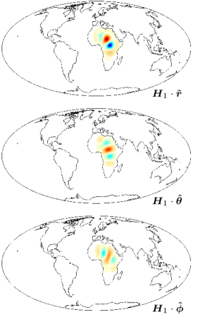
Figure 2: The three vectorial components of the gradient-vector Slepian function $\boldsymbol{H}_{1}$ best concentrated to Africa at a maximum spherical-harmonic degree $L=30$. Top panel shows the radial component $\boldsymbol{H}_{1}\cdot\boldsymbol{\hat{r}}$, center panel the tangential (colatitudinal) component $\boldsymbol{H}_{1}\cdot\boldsymbol{\hat{\theta}}$, and bottom panel the tangential (longitudinal) component $\boldsymbol{H}_{1}\cdot\boldsymbol{\hat{\phi}}$. The concentration coefficient is $\sigma=0.999892$.

We introduce the $(L+1)^{2}\times J$ dimensional matrix containing the $(L+1)^{2}$ gradient-vector spherical-harmonic coefficients for each of the $J$ best-concentrated gradient-vector Slepian functions

$$\mathbf{H}_{J}=\begin{pmatrix}\mathrm{h}_{1}&\cdots&\mathrm{h}_{J}\end{pmatrix},$$ (100)

the $J$-dimensional vector of vector-valued functions containing the $J$ best-concentrated gradient-vector Slepian functions

$$\boldsymbol{\mathcal{H}}_{J}=\mathbf{H}_{J}^{\mathrm{T}}\boldsymbol{\mathcal{E}}=\begin{pmatrix}\boldsymbol{H}_{1}&\cdots&\boldsymbol{H}_{J}\end{pmatrix}^{T},$$ (101)

and the $J\times J$ dimensional diagonal matrix containing the $J$ largest concentration ratios

$$\mathbf{\Sigma}_{J}=\text{diag}(\sigma_{1},\ldots,\sigma_{J})=\int_{R}\boldsymbol{\mathcal{H}}_{J}\cdot\boldsymbol{\mathcal{H}}_{J}^{\mathcal{T}}\,d\Omega.$$ (102)

where the last equality is a consequence of Eqs (93), (95) and (101).

The orthonormality of the $\mathrm{h}_{1},\ldots,\mathrm{h}_{(L+1)^{2}}$ in Eqs (94)–(95) ensures that $\mathbf{H}_{J}^{\mathrm{T}}\mathbf{H}_{J}=\mathbf{I}_{J\times J}$, but the $(L+1)^{2}\times(L+1)^{2}$-dimensional projection matrix $\mathbf{H}_{J}\mathbf{H}_{J}^{\mathrm{T}}$ is not invertible. A local approximation of the gradient function can be obtained from

$$\mbox{\boldmath$\nabla$}V(\boldsymbol{\hat{r}})\approx\sum_{\alpha=1}^{J}t_{\alpha}\boldsymbol{H}_{\alpha}(\boldsymbol{\hat{r}})=\boldsymbol{\mathcal{H}}_{J}^{\mathcal{T}}\mathrm{t}_{J}=\boldsymbol{\mathcal{E}}^{\mathcal{T}}\mathbf{H}_{J}\mathbf{H}_{J}^{\mathrm{T}}\mathrm{v},\qquad\boldsymbol{\hat{r}}\in R.$$ (103)

For use in Section 6.2 we finally define the $\infty\times(L+1)^{2}$-dimensional matrix

$$\hat{\mathbf{K}}_{>L,L}=\int_{R}\hat{\boldsymbol{\mathcal{E}}}_{>L}\cdot\boldsymbol{\mathcal{E}}^{\mathcal{T}}\,d\Omega,$$ (104)

using the notation in Eqs (58)–(59), and from this, we derive an expression for the $J$ components of the spacelimited gradient-vector Slepian functions in the gradient-vector spherical-harmonic basis at degrees larger than $L$,

$$\hat{\boldsymbol{\mathcal{H}}}_{\hat{\boldsymbol{\mathcal{E}}},>L,J}=\hat{\mathbf{H}}_{\hat{\boldsymbol{\mathcal{E}}},>L,J}^{\mathrm{T}}\hat{\boldsymbol{\mathcal{E}}}_{>L}=\mathbf{H}_{J}^{\mathrm{T}}\hat{\mathbf{K}}_{>L,L}^{\mathrm{T}}\hat{\boldsymbol{\mathcal{E}}}_{>L}=\left(\int_{R}\boldsymbol{\mathcal{H}}_{J}\cdot\hat{\boldsymbol{\mathcal{E}}}_{>L}^{\mathcal{T}}\,d\Omega\right)\hat{\boldsymbol{\mathcal{E}}}_{>L}.$$ (105)

The analogy with the scalar Eq. (89) is only partial since the spacelimited versions of $\boldsymbol{\mathcal{H}}$ also have non-vanishing components in the span of $\boldsymbol{F}$ of Eq. (17) and $\boldsymbol{C}$ of Eq. (13) — not just $\boldsymbol{E}$.

5 Potential-Field Estimation from Radial Data Using Slepian Functions

With the scalar Slepian functions defined in Section 4.1 we can now formulate the solution to problem $\mathbf{P2}$ as a localized bandlimited potential-field estimation problem, from noisy radial-derivative data at satellite altitude. More precisely we will use the Slepian functions to localize the radial-field analysis at satellite altitude and then, in a second step, downward transform the resulting spherical-harmonic coefficients using the notions developed in Section 2.3.

As in the exposition of the classical spherical-harmonics based solutions described in Sections 3.1 and 3.2, we start with a description of the numerical estimation procedure based on pointwise data in Section 5.1 before proceeding to a functional formulation that will facilitate the statistical analysis of the performance of the methods, in Section 5.2. Throughout this section we do not assume that the target signal $V(\boldsymbol{\hat{r}})$ is bandlimited, but a bandwidth $L$ does need to be chosen to form the approximation $\tilde{V}(\boldsymbol{\hat{r}})$. The bias that arises from this choice of bandlimitation will be discussed in Section 5.2.

5.1 Discrete Formulation and Truncated Solutions

From pointwise data values of the radial derivative of the potential at satellite altitude, given at the points ${r_{s}}\boldsymbol{\hat{r}}_{1},\ldots,{r_{s}}\boldsymbol{\hat{r}}_{k}$, and polluted by noise,

$$\mathsf{d}_{r}=\mathsf{V}^{\prime}_{r}+\mathsf{n}_{r},$$ (106)

we seek to estimate the bandlimited partial set of corresponding spherical-harmonic coefficients $\mathrm{u}^{r_{e}}=(u_{00}^{r_{e}}\,\cdots\,u_{LL}^{r_{e}})^{T}$ of the scalar potential $V$ on Earth’s surface $\Omega_{r_{e}}$, as in the original statement (35) of Problem $\mathbf{P2}$. In Eq. (106), $\mathsf{V}^{\prime}_{r}$ is defined as in Eq. (33), and $\mathsf{n}_{r}$ is a vector of noise values at the evaluation points.

As seen in Eq. (36), the solution to problem $\mathbf{P2}$ involves the inversion of a “normal” matrix, $(\boldsymbol{\mathsf{Y}}\boldsymbol{\mathsf{Y}}^{\sf T})^{-1}$, that is reminiscent of the localization kernel in Eq. (70), and therefore has many near-zero eigenvalues, and the additional accounting for the effects of altitude via the term $\mathbf{A}^{-1}$, which will potentially unstably inflate the smallest-scale noise terms Maus et al. (2006c). Instead of regularization by damping (in the spherical-harmonic basis), the approach we propose is based on truncation (in the Slepian basis). We focus on the estimation of the radial field at satellite altitude in a chosen target region $R$, by estimating only its $J$ best-concentrated Slepian coefficients. The hard truncation level $J$ is a regularization parameter whose value needs to be chosen based on signal-to-noise considerations and an optimality criterion, much as a proper damping parameter would (Mallat, 2008; Kaula, 1967; Simons & Dahlen, 2006; Wieczorek & Simons, 2007).

Define the $(L+1)^{2}\times k$-dimensional matrix containing the Slepian functions $G_{1},\ldots,G_{(L+1)^{2}}$ evaluated at the latitudinal and longitudinal locations of the data (on the unit sphere),

$$\boldsymbol{\mathsf{G}}=\mathbf{G}^{\mathrm{T}}\boldsymbol{\mathsf{Y}},$$ (107)

where the scalar Slepian transformation matrix $\mathbf{G}$ is defined in Eq. (71). Note the change in (serif vs sans) type. The matrix $\boldsymbol{\mathsf{Y}}$ contains the spherical harmonics evaluated at the data locations on the unit sphere, as in Eq. (28). Problem $\mathbf{P2}$ is restated from its original formulation in Eq. (35) via a bandlimited Slepian transformation at altitude, to

$$\arg\min_{\mathrm{\tilde{u}}^{r_{e}}}\lVert\boldsymbol{\mathsf{Y}}^{\sf T}\mathbf{A}\mathrm{\tilde{u}}^{r_{e}}-\mathsf{d}_{r}\rVert^{2}=\arg\min_{\mathrm{\tilde{u}}^{r_{e}}}\lVert\boldsymbol{\mathsf{Y}}^{\sf T}\mathbf{G}\mathbf{G}^{\mathrm{T}}\mathbf{A}\mathrm{\tilde{u}}^{r_{e}}-\mathsf{d}_{r}\rVert^{2}=\arg\min_{\tilde{\mathrm{s}}^{r_{s}}}\lVert\boldsymbol{\mathsf{G}}^{\sf T}\tilde{\mathrm{s}}^{r_{s}}-\mathsf{d}_{r}\rVert^{2},$$ (108)

where we used the orthogonality $\mathbf{G}\mathbf{G}^{\mathrm{T}}=\mathbf{I}$, the definition Eq. (107), and identified the Slepian expansion coefficients at satellite altitude through transformation of the bandlimited vector (34) into the $(L+1)^{2}$-dimensional vector

$$\tilde{\mathrm{s}}^{r_{s}}=\mathbf{G}^{\mathrm{T}}\mathbf{A}\mathrm{\tilde{u}}^{r_{e}}.$$ (109)

We invoke our regularization of only solving for the coefficients of the $J$ best-concentrated Slepian functions at satellite altitude by defining the $J\times k$ dimensional matrix containing the point evaluations of the $J$ best-concentrated Slepian functions on the unit sphere

$$\boldsymbol{\mathsf{G}}_{J}=\mathbf{G}_{J}^{\mathrm{T}}\boldsymbol{\mathsf{Y}},$$ (110)

and by solving, instead of Eq. (108),

$$\arg\min_{\tilde{\mathrm{s}}^{r_{s}}_{J}}\lVert\boldsymbol{\mathsf{G}}_{J}^{\sf T}\tilde{\mathrm{s}}^{r_{s}}_{J}-\mathsf{d}_{r}\rVert^{2},$$ (111)

for the $J$-dimensional vector $\tilde{\mathrm{s}}^{r_{s}}_{J}$ containing the coefficients of the approximation at satellite altitude in the bandlimited Slepian basis. When $J\leq k$ we have the solution

$$\tilde{\mathrm{s}}^{r_{s}}_{J}=(\boldsymbol{\mathsf{G}}_{J}\boldsymbol{\mathsf{G}}_{J}^{\sf T})^{-1}\boldsymbol{\mathsf{G}}_{J}\mathsf{d}_{r},$$ (112)

which we then downward transform to the $(L+1)^{2}$ spherical-harmonic coefficients $\mathrm{\tilde{u}}^{r_{e}}$ of the field on Earth’s surface $\Omega_{r_{e}}$ as

$$\mathrm{\tilde{u}}^{r_{e}}=\mathbf{A}^{-1}\mathbf{G}_{J}\tilde{\mathrm{s}}^{r_{s}}_{J}=\mathbf{A}^{-1}\mathbf{G}_{J}(\boldsymbol{\mathsf{G}}_{J}\boldsymbol{\mathsf{G}}_{J}^{\sf T})^{-1}\boldsymbol{\mathsf{G}}_{J}\mathsf{d}_{r}\qquad\text{(solution 2 to noisy problem $\mathbf{P2}$)}.$$ (113)

The numerical conditioning of the matrix $(\boldsymbol{\mathsf{G}}_{J}\boldsymbol{\mathsf{G}}_{J}^{\sf T})$ is determined by the truncation parameter $J$, and we require the inverse of the matrix $\mathbf{A}$ defined in Eq. (32).

The resulting approximation $\tilde{V}({r_{e}}\boldsymbol{\hat{r}})$ of the potential field $V({r_{e}}\boldsymbol{\hat{r}})$ at any point of interest on $\Omega_{r_{e}}$ can be calculated as

$$\tilde{V}({r_{e}}\boldsymbol{\hat{r}})=\mathcal{Y}^{\mathcal{T}}\mathrm{\tilde{u}}^{r_{e}}=\mathcal{G}_{\downarrow J}^{\mathcal{T}}(\boldsymbol{\mathsf{G}}_{J}\boldsymbol{\mathsf{G}}_{J}^{\sf T})^{-1}\boldsymbol{\mathsf{G}}_{J}\mathsf{d}_{r}=\mathcal{G}_{\downarrow J}^{\mathcal{T}}\tilde{\mathrm{s}}^{r_{s}}_{J},$$ (114)

where we have defined the vector of the $J$ best-concentrated (and its complement) downward-transformed scalar Slepian functions as

$$\mathcal{G}_{\downarrow J}=\mathbf{G}_{J}^{\mathrm{T}}\mathbf{A}^{-1}\mathcal{Y},\qquad\mathcal{G}_{\downarrow>J}=\mathbf{G}_{>J}^{\mathrm{T}}\mathbf{A}^{-1}\mathcal{Y},$$ (115)

an example of which is plotted in Fig. 3. We reserve for later use the vectors of upward-transformed Slepian functions,

$$\mathcal{G}_{\uparrow J}=\mathbf{G}_{J}^{\mathrm{T}}\mathbf{A}\mathcal{Y},\qquad\mathcal{G}_{\uparrow>J}=\mathbf{G}_{>J}^{\mathrm{T}}\mathbf{A}\mathcal{Y}.$$ (116)

From Eqs (115)–(116) and (71) or (75) we also obtain the equivalencies

$$\mathcal{G}_{\downarrow}^{\mathcal{T}}(\boldsymbol{\hat{r}})\hskip 1.00006pt\mathcal{G}_{\uparrow}(\boldsymbol{\hat{r}}^{\prime})=\mathcal{Y}^{\mathcal{T}}(\boldsymbol{\hat{r}})\hskip 1.00006pt\mathbf{A}^{-1}\mathbf{G}\mathbf{G}^{\mathrm{T}}\hskip 1.00006pt\mathbf{A}\mathcal{Y}(\boldsymbol{\hat{r}}^{\prime})=\mathcal{Y}^{\mathcal{T}}(\boldsymbol{\hat{r}})\mathcal{Y}(\boldsymbol{\hat{r}}^{\prime})=\mathcal{G}^{\mathcal{T}}(\boldsymbol{\hat{r}})\hskip 1.00006pt\mathcal{G}(\boldsymbol{\hat{r}}^{\prime}),$$ (117)

in the “silent” $J=(L+1)^{2}$ notation of Eq. (75), but noting that Eq. (117) does have an equivalent in truncated form when $J\neq(L+1)^{2}$. Evidently, we also have

$$\mathcal{G}_{\downarrow}^{\mathcal{T}}\mathcal{G}_{\uparrow}=\mathcal{G}_{\downarrow J}^{\mathcal{T}}\mathcal{G}_{\uparrow J}+\mathcal{G}_{\downarrow>J}^{\mathcal{T}}\mathcal{G}_{\uparrow>J}.$$ (118)

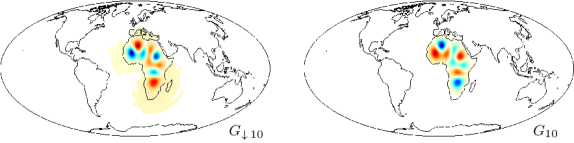
Figure 3: Downward transformation of the 10th best-concentrated scalar Slepian function for Africa and a maximum spherical-harmonic degree $L=30$. The right panel shows the concentrated scalar Slepian function $G_{10}=\mathcal{Y}^{\mathcal{T}}\mathrm{g}_{10}$ for the radial component at an altitude of 500 km. The left panel shows the equivalent downward-transformed function $G_{\downarrow\,10}=\mathcal{Y}^{\mathcal{T}}\mathbf{A}^{-1}\mathrm{g}_{10}$ to describe a scalar potential on Earth’s surface (${r_{e}}=6371$ km). The concentration coefficient for the Slepian function $G_{10}$ at altitude is $\lambda=0.99985$.

5.2 Continuous Formulation and Statistical Considerations

In this section we provide a formulation of the approach described in Section 5.1 that considers the data in their functional form instead of being given as point values. In this formalism we will then express the estimation variance, bias, and mean squared error for the methods presented under some special cases. Our results will generalize the scalar treatment of Simons & Dahlen (2006) in whose work we will point out a misprint that we correct here.

5.2.1 Continuous Formulation

The analytical counterpart to the pointwise data from Eq. (106) known (or desired) only within the target region $R$ is

$$d(\boldsymbol{\hat{r}})=\begin{cases}\partial_{r}V({r_{s}}\boldsymbol{\hat{r}})+n(\boldsymbol{\hat{r}})&\text{if }\boldsymbol{\hat{r}}\in R\\ \text{unknown}&\text{if }\boldsymbol{\hat{r}}\in\Omega\setminus R,\end{cases}$$ (119)

where $n(\boldsymbol{\hat{r}})$ is the spatial noise function. The estimation problem equivalent to Eq. (108) can now be formulated as

$$\arg\min_{\mathrm{\tilde{u}}^{r_{e}}}\int_{R}{\left(\mathcal{Y}^{\mathcal{T}}\mathbf{A}\mathrm{\tilde{u}}^{r_{e}}-d\right)^{2}}\,d\Omega=\arg\min_{\mathrm{\tilde{u}}^{r_{e}}}\int_{R}{\left(\mathcal{Y}^{\mathcal{T}}\mathbf{G}\mathbf{G}^{\mathrm{T}}\mathbf{A}\mathrm{\tilde{u}}^{r_{e}}-d\right)^{2}}\,d\Omega=\arg\min_{\tilde{\mathrm{s}}^{r_{s}}}\int_{R}{\left(\mathcal{G}^{\mathcal{T}}\tilde{\mathrm{s}}^{r_{s}}-d\right)^{2}}\,d\Omega,$$ (120)

where the vector of Slepian functions $\mathcal{G}$ is defined in Eq. (75) and the estimated coefficients at satellite altitude $\tilde{\mathrm{s}}^{r_{s}}$ are in Eq. (109). The problem is regularized by solving exclusively for the $J$ best-concentrated Slepian coefficients that describe the data in Eq. (119), which transforms Eq. (120) into the estimation problem

$$\arg\min_{\tilde{\mathrm{s}}^{r_{s}}_{J}}\int_{R}{\left(\mathcal{G}_{J}^{\mathcal{T}}\tilde{\mathrm{s}}^{r_{s}}_{J}-d\right)^{2}}\,d\Omega.$$ (121)

Differentiating with respect to $\tilde{\mathrm{s}}^{r_{s}}_{J}$ to find the stationary points, and making use of Eq. (79), the solution is given by

$$\tilde{\mathrm{s}}^{r_{s}}_{J}=\left(\int_{R}\mathcal{G}_{J}\mathcal{G}_{J}^{\mathcal{T}}\,d\Omega\right)^{-1}\int_{R}\mathcal{G}_{J}d\,d\Omega=\mathbf{\Lambda}_{J}^{-1}\int_{R}\mathcal{G}_{J}d\,d\Omega.$$ (122)

As with the estimation of the spherical-harmonic coefficients of the potential field from the Slepian coefficients at altitude obtained from pointwise data in Eq. (113) we can estimate the vector containing the $(L+1)^{2}$ spherical-harmonic coefficients $\mathrm{\tilde{u}}^{r_{e}}$ from the $J$-dimensional vector of Slepian coefficients $\tilde{\mathrm{s}}^{r_{s}}_{J}$ by first transforming it to the $(L+1)^{2}$-dimensional vector of spherical-harmonic coefficients $\mathbf{G}_{J}\tilde{\mathrm{s}}^{r_{s}}_{J}$ and then downward transforming it using the matrix $\mathbf{A}$ defined in Eq. (32). We thereby obtain the spherical-harmonic coefficients $\mathrm{\tilde{u}}^{r_{e}}$ for the estimation $\tilde{V}({r_{e}}\boldsymbol{\hat{r}})$ of the potential field on Earth’s surface $\Omega_{r_{e}}$ as

$$\mathrm{\tilde{u}}^{r_{e}}=\mathbf{A}^{-1}\mathbf{G}_{J}\mathbf{\Lambda}^{-1}_{J}\int_{R}\mathcal{G}_{J}d\,d\Omega\qquad(\text{analytical solution 2 to problem $\mathbf{P2}$}).$$ (123)

We can expand the coefficients $\mathrm{\tilde{u}}^{r_{e}}$ obtained from the data $d$ by Eq. (123) to evaluate the potential field anywhere on Earth’s surface as

$$\tilde{V}({r_{e}}\boldsymbol{\hat{r}})=\mathcal{Y}^{\mathcal{T}}\mathrm{\tilde{u}}^{r_{e}}=\mathcal{Y}^{\mathcal{T}}\mathbf{A}^{-1}\mathbf{G}_{J}\mathbf{\Lambda}^{-1}_{J}\int_{R}\mathcal{G}_{J}d\,d\Omega=\mathcal{G}_{\downarrow J}^{\mathcal{T}}\mathbf{\Lambda}^{-1}_{J}\int_{R}\mathcal{G}_{J}d\,d\Omega,$$ (124)

where the truncated vector of downward transformed Slepian functions $\mathcal{G}_{\downarrow J}$ is defined in Eq. (115).

5.2.2 Effects of Bandlimiting the Scalar Estimates

The estimate given in Eq. (124) has a bandlimited representation of the unknown potential at its heart, though the actual potential that we are attempting to estimate will generally not be bandlimited, see Eqs (18) and (27), nor will the noise be. To isolate the effects of the bandlimitation, we write the data as the sum of a bandlimited part (which is expanded globally in Slepian functions of the same bandwidth), its wideband complement, which contains spherical harmonics with degree greater than $L$ introduced in Eq. (52), and the noise contribution. Eq. (119) then becomes

$$d=\partial_{r}V({r_{s}}\boldsymbol{\hat{r}})+n=\mathcal{G}^{\mathcal{T}}\int_{\Omega}\mathcal{G}\hskip 1.00006pt\partial_{r}V({r_{s}}\boldsymbol{\hat{r}})\,d\Omega+\hat{\mathcal{Y}}_{>L}^{\mathcal{T}}\int_{\Omega}\hat{\mathcal{Y}}_{>L}\partial_{r}V({r_{s}}\boldsymbol{\hat{r}})\,d\Omega+n.$$ (125)

To this we apply the integral transform of Eq. (124) using the $J$ best-concentrated Slepian functions $\mathcal{G}_{J}$, and we make use of the orthogonality Eq. (74), Eqs (78)–(79) and Eq. (89), to obtain the expression

$$\int_{R}\mathcal{G}_{J}d\,d\Omega =\int_{R}\mathcal{G}_{J}\mathcal{G}^{\mathcal{T}}\,d\Omega\int_{\Omega}\mathcal{G}\hskip 1.00006pt\partial_{r}V({r_{s}}\boldsymbol{\hat{r}})\,d\Omega+\int_{R}\mathcal{G}_{J}\hat{\mathcal{Y}}_{>L}^{\mathcal{T}}\,d\Omega\int_{\Omega}\hat{\mathcal{Y}}_{>L}\partial_{r}V({r_{s}}\boldsymbol{\hat{r}})\,d\Omega+\int_{R}\mathcal{G}_{J}\hskip 1.00006ptn\,d\Omega$$ (126)

$$=\mathbf{\Lambda}_{J}\int_{\Omega}\mathcal{G}_{J}\partial_{r}V({r_{s}}\boldsymbol{\hat{r}})\,d\Omega+\mathbf{G}_{J}^{\mathrm{T}}\hat{\mathbf{D}}_{>L,L}^{\mathrm{T}}\int_{\Omega}\hat{\mathcal{Y}}_{>L}\partial_{r}V({r_{s}}\boldsymbol{\hat{r}})\,d\Omega+\int_{R}\mathcal{G}_{J}n\,d\Omega$$ (127)

$$=\mathbf{\Lambda}_{J}\int_{\Omega}\mathcal{G}_{J}\partial_{r}V({r_{s}}\boldsymbol{\hat{r}})\,d\Omega+\hat{\mathbf{G}}_{>L,J}^{\mathrm{T}}\int_{\Omega}\hat{\mathcal{Y}}_{>L}\partial_{r}V({r_{s}}\boldsymbol{\hat{r}})\,d\Omega+\int_{R}\mathcal{G}_{J}n\,d\Omega$$ (128)

$$=\mathbf{\Lambda}_{J}\int_{\Omega}\mathcal{G}_{J}\partial_{r}V({r_{s}}\boldsymbol{\hat{r}})\,d\Omega+\int_{\Omega}\hat{\mathcal{G}}_{>L,J}\partial_{r}V({r_{s}}\boldsymbol{\hat{r}})\,d\Omega+\int_{R}\mathcal{G}_{J}n\,d\Omega.$$ (129)

Finally we can insert the result (129) into Eq. (124) to discover the contributions to the bandlimited estimate $\tilde{V}({r_{e}}\boldsymbol{\hat{r}})$ from signal with energy in the spherical-harmonic degree range $l>L$ and the presence of noise:

$$\tilde{V}({r_{e}}\boldsymbol{\hat{r}})=\mathcal{G}_{\downarrow J}^{\mathcal{T}}\int_{\Omega}\mathcal{G}_{J}\partial_{r}V({r_{s}}\boldsymbol{\hat{r}})\,d\Omega+\mathcal{G}_{\downarrow J}^{\mathcal{T}}\mathbf{\Lambda}^{-1}_{J}\left(\int_{\Omega}\hat{\mathcal{G}}_{>L,J}\partial_{r}V({r_{s}}\boldsymbol{\hat{r}})\,d\Omega+\int_{R}\mathcal{G}_{J}\hskip 1.00006ptn\,d\Omega\right),$$ (130)

an expression equivalent to eq. (136) of Simons & Dahlen (2006). Ultimately, Eq. (130) is derived from an estimate of the spherical-harmonic potential coefficients, Eq. (123), that uses a truncated (to $J$) set of bandlimited (to $L$) spatially concentrated (to $R$) Slepian functions. Keeping with the terminology introduced by Simons & Dahlen (2006), the truncation bias in the bandlimited part of the estimate (the first right-hand-side term in Eq. 130) diminishes as $J$ increases, but the second, parenthetical, term grows, very unfavorably fast, with the inverse-eigenvalue matrix $\mathbf{\Lambda}_{J}^{-1}$. This term contains the broadband leakage, which is captured from the non-bandlimited part of the signal by the nonvanishing regional product integral in the second term of Eq. (126), and the contribution due to the noise in the region over which data are available. Comparison of the bandlimited estimate (130) with the wideband original form (27) will furthermore identify a broadband bias that arises from the outright neglect of the necessary basis functions, and is thus, essentially, unavoidable. The broadband leakage can be controlled under some theoretical or numerical schemes (e.g. Hwang, 1993; Trampert & Snieder, 1996; Albertella et al., 2008). Oftentimes, however, those fail to be practically successful at the desired level of accuracy of the solution (e.g. Slobbe et al., 2012).

5.2.3 Statistical Analysis for Scalar Bandlimited-White Processes

The complete assessment of the statistical performance of the estimators (123)–(124) is an ambitious objective. It is difficult to go beyond Eq. (130) without making detailed assumptions about the underlying statistics of both signal and noise, not to mention the specifics of the region of data coverage and the satellite altitude (e.g. Kaula, 1967; Whaler & Gubbins, 1981; Xu, 1992a, b, 1998; Schachtschneider et al., 2010, 2012; Slobbe et al., 2012). However, as shown by Simons & Dahlen (2006), special cases are easy to come by and learn from. We recall the standard definitions for the estimation error, bias and variance,

$$\epsilon =\tilde{V}({r_{e}}\boldsymbol{\hat{r}})-V({r_{e}}\boldsymbol{\hat{r}}),$$ (131)

$$\beta =\big{\langle}\tilde{V}({r_{e}}\boldsymbol{\hat{r}})\big{\rangle}-V({r_{e}}\boldsymbol{\hat{r}}),$$ (132)

$$\nu =\big{\langle}\tilde{V}^{2}({r_{e}}\boldsymbol{\hat{r}})\big{\rangle}-\big{\langle}\tilde{V}({r_{e}}\boldsymbol{\hat{r}})\big{\rangle}^{2},$$ (133)

and, typically the quantity to be minimized, the mean squared error:

$$\langle\epsilon^{2}\rangle=\nu+\langle\beta^{2}\rangle.$$ (134)

The angular brackets in Eq. (134) refer to averaging over a hypothetical ensemble of repeated observations, treating both signal and noise as stochastic processes (see Simons & Dahlen, 2006). We make the following four oversimplified assumptions by which to obtain simple and insightful expressions for $\nu,\beta$, and $\langle\epsilon^{2}\rangle$:

1. The signal $V({r_{e}}\boldsymbol{\hat{r}})$ is bandlimited, as are the Slepian functions $\mathcal{G}$, with the same bandwidth $L$.

2. The signal is — almost, given the incompatible stipulation 1 — “white” on Earth’s surface, with power $S$, in the sense $\langle V({r_{e}}\boldsymbol{\hat{r}})V({r_{e}}\boldsymbol{\hat{r}}^{\prime})\rangle=S\hskip 1.00006pt\delta(\boldsymbol{\hat{r}},\boldsymbol{\hat{r}}^{\prime})$, and with $\delta(\boldsymbol{\hat{r}},\boldsymbol{\hat{r}}^{\prime})$ the scalar spherical delta function (see Simons et al., 2006).

3. The noise is white at the observation level, with power $N$, as $\langle n(\boldsymbol{\hat{r}})n(\boldsymbol{\hat{r}}^{\prime})\rangle=N\delta(\boldsymbol{\hat{r}},\boldsymbol{\hat{r}}^{\prime})$.

4. The noise has zero mean and is uncorrelated with the signal, $\langle n(\boldsymbol{\hat{r}})\rangle=0=\langle n(\boldsymbol{\hat{r}})V(\boldsymbol{\hat{r}}^{\prime})\rangle$.

To honor 1 we insert the bandwidth-restricted version of Eq. (57) into Eq. (130), observe the cancellation, via the whole-sphere orthogonality of $\hat{\mathcal{G}}_{>L}$ and $\mathcal{Y}$, of the first term inside of the parentheses in Eq. (130), and then apply the relation (78) and the orthogonality (71), to arrive at

$$\tilde{V}({r_{e}}\boldsymbol{\hat{r}}) =\mathcal{G}_{\downarrow J}^{\mathcal{T}}\left(\int_{\Omega}\mathcal{G}_{J}\mathcal{Y}^{\mathcal{T}}\mathbf{A}\mathrm{u}^{r_{e}}\,d\Omega+\mathbf{\Lambda}^{-1}_{J}\int_{R}\mathcal{G}_{J}\hskip 1.00006ptn\,d\Omega\right)=\mathcal{G}_{\downarrow J}^{\mathcal{T}}\left(\mathbf{G}_{J}^{\mathrm{T}}\mathbf{A}\mathrm{u}^{r_{e}}+\mathbf{\Lambda}^{-1}_{J}\int_{R}\mathcal{G}_{J}\hskip 1.00006ptn\,d\Omega\right)$$

$$=\mathcal{G}_{\downarrow J}^{\mathcal{T}}\left(\int_{\Omega}\mathcal{G}_{\uparrow J}V({r_{e}}\boldsymbol{\hat{r}})\,d\Omega+\mathbf{\Lambda}^{-1}_{J}\int_{R}\mathcal{G}_{J}\hskip 1.00006ptn\,d\Omega\right).$$ (135)

The last equality follows from the bandlimited identification $V({r_{e}}\boldsymbol{\hat{r}})=\mathcal{Y}^{\mathcal{T}}\mathrm{u}^{r_{e}}$ as from Eq. (56), global orthogonality of the $\mathcal{Y}$, and by substitution of Eq. (116). From Eqs (117)–(118) we furthermore know that the unknown bandlimited signal $V({r_{e}}\boldsymbol{\hat{r}})$ can be represented using the up- and downward transformed Slepian functions as

$$V({r_{e}}\boldsymbol{\hat{r}})=\mathcal{G}_{\downarrow}^{\mathcal{T}}\int_{\Omega}\mathcal{G}_{\uparrow}V({r_{e}}\boldsymbol{\hat{r}})\,d\Omega=\mathcal{G}_{\downarrow J}^{\mathcal{T}}\int_{\Omega}\mathcal{G}_{\uparrow J}V({r_{e}}\boldsymbol{\hat{r}})\,d\Omega+\mathcal{G}_{\downarrow>J}^{\mathcal{T}}\int_{\Omega}\mathcal{G}_{\uparrow>J}V({r_{e}}\boldsymbol{\hat{r}})\,d\Omega.$$ (136)

We can now calculate the bias $\beta$ from Eq. (132) by applying the averaging operation to Eq. (135), using assumption 4, and then subtracting Eq. (136), to give the result, which grows with diminishing truncation $J$,

$$\beta=-\mathcal{G}_{\downarrow>J}^{\mathcal{T}}\int_{\Omega}\mathcal{G}_{\uparrow>J}V({r_{e}}\boldsymbol{\hat{r}})\,d\Omega.$$ (137)

In order to calculate the variance $\nu$ we use Eq. (135) to obtain the squared

$$\tilde{V}^{2}({r_{e}}\boldsymbol{\hat{r}}) =\mathcal{G}_{\downarrow J}^{\mathcal{T}}\left(\int_{\Omega}\mathcal{G}_{\uparrow J}V({r_{e}}\boldsymbol{\hat{r}})\,d\Omega+\mathbf{\Lambda}^{-1}_{J}\int_{R}\mathcal{G}_{J}\hskip 1.00006ptn\,d\Omega\right)\left(\int_{\Omega}V({r_{e}}\boldsymbol{\hat{r}})\hskip 1.00006pt\mathcal{G}_{\uparrow J}^{\mathcal{T}}\,d\Omega+\mathbf{\Lambda}^{-1}_{J}\int_{R}n\hskip 1.00006pt\mathcal{G}_{J}^{\mathcal{T}}\,d\Omega\right)\mathcal{G}_{\downarrow J}$$ (138)

$$=\mathcal{G}_{\downarrow J}^{\mathcal{T}}\left(\int_{\Omega}\int_{\Omega}\mathcal{G}_{\uparrow J}(\boldsymbol{\hat{r}})V({r_{e}}\boldsymbol{\hat{r}})V({r_{e}}\boldsymbol{\hat{r}}^{\prime})\hskip 1.00006pt\mathcal{G}_{\uparrow J}^{\mathcal{T}}(\boldsymbol{\hat{r}}^{\prime})\,d\Omega^{\prime}\,d\Omega\right.+\mathbf{\Lambda}^{-1}_{J}\int_{R}\int_{R}\mathcal{G}_{J}(\boldsymbol{\hat{r}})\hskip 1.00006ptn(\boldsymbol{\hat{r}})n(\boldsymbol{\hat{r}}^{\prime})\hskip 1.00006pt\mathcal{G}_{J}^{\mathcal{T}}(\boldsymbol{\hat{r}}^{\prime})\,d\Omega^{\prime}\,d\Omega\hskip 1.00006pt\mathbf{\Lambda}^{-1}_{J}$$

$$\left.\qquad+\int_{\Omega}\int_{R}\mathcal{G}_{\uparrow J}(\boldsymbol{\hat{r}})V({r_{e}}\boldsymbol{\hat{r}})n(\boldsymbol{\hat{r}}^{\prime})\hskip 1.00006pt\mathcal{G}_{J}^{\mathcal{T}}(\boldsymbol{\hat{r}}^{\prime})\,d\Omega^{\prime}\,d\Omega\hskip 1.00006pt\mathbf{\Lambda}^{-1}_{J}+\mathbf{\Lambda}^{-1}_{J}\int_{R}\int_{\Omega}\mathcal{G}_{J}(\boldsymbol{\hat{r}})\hskip 1.00006ptn(\boldsymbol{\hat{r}})V({r_{e}}\boldsymbol{\hat{r}}^{\prime})\hskip 1.00006pt\mathcal{G}_{\uparrow J}^{\mathcal{T}}(\boldsymbol{\hat{r}}^{\prime})\,d\Omega^{\prime}\,d\Omega\right)\mathcal{G}_{\downarrow J}.$$ (139)

We apply the averaging over the different realizations of the noise in Eq. (5.2.3), and use assumptions 3–4 and Eq. (79), from which we subtract the square of the average of Eq. (135) to obtain the variance in Eq. (133), which grows with $J$, as

$$\nu=N\mathcal{G}_{\downarrow J}^{\mathcal{T}}\mathbf{\Lambda}_{J}^{-1}\mathcal{G}_{\downarrow J}.$$ (140)

The squared bias averaged over all realizations of the signal, using assumption 2, making the substitution (116), and using the whole-sphere orthogonality (71) of the spherical harmonics $\mathcal{Y}$, yields

$$\langle\beta^{2}\rangle=S\hskip 1.00006pt\mathcal{G}_{\downarrow>J}^{\mathcal{T}}\big{(}\mathbf{G}_{>J}^{\mathrm{T}}\mathbf{A}^{2}\mathbf{G}_{>J}\big{)}\hskip 1.00006pt\mathcal{G}_{\downarrow>J},$$ (141)

which leads, together with the variance in Eq. (140), via Eq. (134) to the mean squared estimation error

$$\langle\epsilon^{2}\rangle=N\mathcal{G}_{\downarrow J}^{\mathcal{T}}\mathbf{\Lambda}_{J}^{-1}\mathcal{G}_{\downarrow J}+S\hskip 1.00006pt\mathcal{G}_{\downarrow>J}^{\mathcal{T}}\big{(}\mathbf{G}_{>J}^{\mathrm{T}}\mathbf{A}^{2}\mathbf{G}_{>J}\big{)}\hskip 1.00006pt\mathcal{G}_{\downarrow>J}.$$ (142)

With Eqs (137), (141) and (142) we correct Eqs (143)–(145) of Simons & Dahlen (2006). We can understand their typo by writing Eq. (141) using Eq. (115) as $\langle\beta^{2}\rangle=S\mathcal{Y}^{\mathcal{T}}\mathbf{A}^{-1}\mathbf{G}_{>J}\mathbf{G}_{>J}^{\mathrm{T}}\mathbf{A}^{2}\mathbf{G}_{>J}\mathbf{G}_{>J}^{\mathrm{T}}\mathbf{A}^{-1}\mathcal{Y}$ and recognizing that the terms $\mathbf{G}_{>J}\mathbf{G}_{>J}^{\mathrm{T}}$ are never identities, and that the interior term $\mathbf{G}_{>J}^{\mathrm{T}}\mathbf{A}^{2}\mathbf{G}_{>J}$ is an identity only when $\mathbf{A}$ itself is an identity, which is never the case in this chapter, but would apply in the zero-altitude scalar case considered by Simons & Dahlen (2006). Another way of stating it is that Simons & Dahlen (2006) mistakenly applied their identity (93), which is our (117), in the case of truncated sums, for which it does not hold. The typos do not affect any of their further analysis or conclusions, which were conducted at zero altitude.

6 Potential-Field Estimation from Vectorial Data Using Slepian Functions

In this section we present a method to solve problem $\mathbf{P4}$, the estimation of the potential field on Earth’s surface from noisy (three-component) vectorial data at satellite altitude (e.g. Arkani-Hamed, 2002). The method is constructed in a similar fashion to the scalar solutions to problem $\mathbf{P2}$ described in Section 5. We will use the gradient-vector Slepian functions introduced in Section 4.2 to fit the local data at satellite altitude and then downward transform the gradient-vector spherical harmonic coefficients thus obtained. As for the scalar case we will first present the numerical method applicable to pointwise data and then develop a functional formulation that will allow us to analyze the effect of non-bandlimited signal and noise on the estimation.

6.1 Discrete Formulation and Truncated Solutions

Given pointwise data values of the gradient of the potential that are polluted by noise at the points ${r_{s}}\boldsymbol{\hat{r}}_{1},\ldots,{r_{s}}\boldsymbol{\hat{r}}_{k}$,

$$\mathsf{d}=\mathsf{V}^{\prime}+\mathsf{n},$$ (143)

where $\mathsf{V}^{\prime}$ is defined in Eq. (38), and $\mathsf{n}$ is a vector of noise values at the evaluation points for the individual components, we seek to estimate the spherical-harmonic coefficients $\mathrm{u}^{r_{e}}=(u_{00}^{r_{e}}\,\cdots\,u_{LL}^{r_{e}})^{T}$ of the scalar potential $V$ on Earth’s surface $\Omega_{r_{e}}$, as in the statement (49) of problem $\mathbf{P4}$. The solution Eq. (50) contains the matrix inverse $(\boldsymbol{\mathsf{E}}\boldsymbol{\mathsf{E}}^{\sf T})^{-1}$ which, like its counterpart Eq. (93), is intrinsically poorly conditioned. To regularize the problem we transform the problem into the gradient-vector Slepian basis for the relevant bandwidth and the chosen target region $R$, and focus on estimating only the $J$ best-concentrated gradient-vector Slepian coefficients. We leave the choice of the value $J$ for later.

We define the $(L+1)^{2}\times 3k$ dimensional matrix containing the $(L+1)^{2}$ gradient-vector Slepian functions $\boldsymbol{H}_{1},\ldots,\boldsymbol{H}_{(L+1)^{2}}$ evaluated at the unit-sphere longitudes and latitudes of the data,

$$\boldsymbol{\mathsf{H}}=\mathbf{H}^{\mathrm{T}}\boldsymbol{\mathsf{E}},$$ (144)

where the gradient-vector Slepian transformation matrix $\mathbf{H}$ is defined in Eq. (94) and the matrix $\boldsymbol{\mathsf{E}}$ containing the values of the gradient-vector spherical harmonics evaluated at the data locations on the unit sphere is defined in Eq. (42). Problem $\mathbf{P4}$ is rewritten from Eq. (49) via the gradient-vector Slepian transformation $\mathbf{H}$ at altitude, to

$$\arg\min_{\mathrm{\tilde{u}}^{r_{e}}}\lVert\boldsymbol{\mathsf{E}}^{\sf T}\mathbf{B}\mathrm{\tilde{u}}^{r_{e}}-\mathsf{d}\rVert^{2}=\arg\min_{\mathrm{\tilde{u}}^{r_{e}}}\lVert\boldsymbol{\mathsf{E}}^{\sf T}\mathbf{H}\mathbf{H}^{\mathrm{T}}\mathbf{B}\mathrm{\tilde{u}}^{r_{e}}-\mathsf{d}\rVert^{2}=\arg\min_{{\tilde{\mathrm{t}}}^{r_{s}}}\lVert\boldsymbol{\mathsf{H}}^{\sf T}{\tilde{\mathrm{t}}}^{r_{s}}-\mathsf{d}\rVert^{2},$$ (145)

where we used the orthogonality $\mathbf{H}\mathbf{H}^{\mathrm{T}}=\mathbf{I}$, the definition Eq. (144) and introduced the gradient-vector Slepian coefficients at satellite altitude

$${\tilde{\mathrm{t}}}^{r_{s}}=\mathbf{H}^{\mathrm{T}}\mathbf{B}\mathrm{\tilde{u}}^{r_{e}}.$$ (146)

As for the scalar case we apply regularization by only estimating the coefficients for the $J$ best-concentrated gradient-vector Slepian functions. We define the $J\times 3k$ dimensional matrix containing the point evaluations of those,

$$\boldsymbol{\mathsf{H}}_{J}=\mathbf{H}_{J}^{\mathrm{T}}\boldsymbol{\mathsf{E}}$$ (147)

and then solve

$$\arg\min_{{\tilde{\mathrm{t}}}^{r_{s}}_{J}}\lVert\boldsymbol{\mathsf{H}}_{J}^{\sf T}{\tilde{\mathrm{t}}}^{r_{s}}_{J}-\mathsf{d}\rVert^{2}$$ (148)

for the $J$-dimensional vector ${\tilde{\mathrm{t}}}^{r_{s}}_{J}$ of gradient-vector Slepian coefficients at satellite altitude. For $J\leq 3k$ the minimizer

$${\tilde{\mathrm{t}}}^{r_{s}}_{J}=(\boldsymbol{\mathsf{H}}_{J}\boldsymbol{\mathsf{H}}_{J}^{\sf T})^{-1}\boldsymbol{\mathsf{H}}_{J}\mathsf{d}$$ (149)

is subsequently downward transformed to the $(L+1)^{2}$ spherical-harmonic coefficients $\mathrm{\tilde{u}}^{r_{e}}$ of the field on Earth’s surface $\Omega_{r_{e}}$ as

$$\mathrm{\tilde{u}}^{r_{e}}=\mathbf{B}^{-1}\mathbf{H}_{J}{\tilde{\mathrm{t}}}^{r_{s}}_{J}=\mathbf{B}^{-1}\mathbf{H}_{J}(\boldsymbol{\mathsf{H}}_{J}\boldsymbol{\mathsf{H}}_{J}^{\sf T})^{-1}\boldsymbol{\mathsf{H}}_{J}\mathsf{d}\qquad\text{(solution 2 to noisy problem $\mathbf{P4}$)},$$ (150)

using matrix $\mathbf{B}$ defined in Eq. (48). The conditioning of the matrix $(\boldsymbol{\mathsf{H}}_{J}\boldsymbol{\mathsf{H}}_{J}^{\sf T})$ is determined by the truncation level $J$. The local approximation $\tilde{V}({r_{e}}\boldsymbol{\hat{r}})$ of the potential field $V({r_{e}}\boldsymbol{\hat{r}})$ can now be calculated by

$$\tilde{V}({r_{e}}\boldsymbol{\hat{r}})=\mathcal{Y}^{\mathcal{T}}\mathrm{\tilde{u}}^{{r_{e}}}=\mathcal{H}^{\mathcal{T}}_{\downarrow J}(\boldsymbol{\mathsf{H}}_{J}\boldsymbol{\mathsf{H}}_{J}^{\sf T})^{-1}\boldsymbol{\mathsf{H}}_{J}\mathsf{d}=\mathcal{H}^{\mathcal{T}}_{\downarrow J}{\tilde{\mathrm{t}}}^{r_{s}}_{J},$$ (151)

where we have defined the vector of the $J$ best-concentrated gradient vector Slepian functions (and its complement) that are downward transformed (hence, expanded in scalar spherical harmonics) as

$$\mathcal{H}_{\downarrow J}=\mathbf{H}_{J}^{\mathrm{T}}\mathbf{B}^{-1}\mathcal{Y},\qquad\mathcal{H}_{\downarrow>J}=\mathbf{H}_{>J}^{\mathrm{T}}\mathbf{B}^{-1}\mathcal{Y}.$$ (152)

Fig. 4 shows an example. Similarly, we will be needing the upward-transformed pair of vectors

$$\mathcal{H}_{\uparrow J}=\mathbf{H}_{J}^{\mathrm{T}}\mathbf{B}\mathcal{Y},\qquad\mathcal{H}_{\uparrow>J}=\mathbf{H}_{>J}^{\mathrm{T}}\mathbf{B}\mathcal{Y},$$ (153)

and the relation derived from them when $J=(L+1)^{2}$ and Eq. (94) or Eq. (98), the equivalent of Eq. (117), namely

$$\mathcal{H}_{\downarrow}^{\mathcal{T}}(\boldsymbol{\hat{r}})\hskip 1.00006pt\mathcal{H}_{\uparrow}(\boldsymbol{\hat{r}}^{\prime})=\mathcal{Y}^{\mathcal{T}}(\boldsymbol{\hat{r}})\hskip 1.00006pt\mathbf{B}^{-1}\mathbf{H}\mathbf{H}^{\mathrm{T}}\hskip 1.00006pt\mathbf{B}\hskip 1.00006pt\mathcal{Y}(\boldsymbol{\hat{r}}^{\prime})=\mathcal{Y}^{\mathcal{T}}(\boldsymbol{\hat{r}})\mathcal{Y}(\boldsymbol{\hat{r}}^{\prime})=\mathcal{H}^{\mathcal{T}}(\boldsymbol{\hat{r}})\hskip 1.00006pt\mathcal{H}(\boldsymbol{\hat{r}}^{\prime}).$$ (154)

Once again we stress that we cannot derive such an equality after any truncation of the Slepian function set. We do have

$$\mathcal{H}_{\downarrow}^{\mathcal{T}}(\boldsymbol{\hat{r}})\hskip 1.00006pt\mathcal{H}_{\uparrow}(\boldsymbol{\hat{r}}^{\prime})=\mathcal{H}_{\downarrow J}^{\mathcal{T}}(\boldsymbol{\hat{r}})\hskip 1.00006pt\mathcal{H}_{\uparrow J}(\boldsymbol{\hat{r}}^{\prime})+\mathcal{H}_{\downarrow>J}^{\mathcal{T}}(\boldsymbol{\hat{r}})\hskip 1.00006pt\mathcal{H}_{\uparrow>J}(\boldsymbol{\hat{r}}^{\prime}).$$ (155)

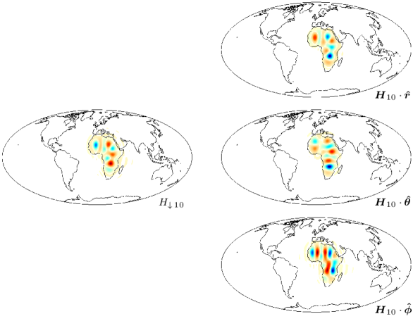
Figure 4: Downward transformation of the 10th best-concentrated gradient-vector Slepian function for Africa and a maximum spherical-harmonic degree $L=30$. The right panels show the concentrated gradient-vector Slepian function $\boldsymbol{H}_{10}=\boldsymbol{\mathcal{E}}^{\mathcal{T}}\mathrm{h}_{10}$. Top right panel shows the radial component $\boldsymbol{H}_{10}\cdot\boldsymbol{\hat{r}}$, middle right panel the tangential (colatitudinal) component $\boldsymbol{H}_{10}\cdot\boldsymbol{\hat{\theta}}$, and the lower right panel the tangential (longitudinal) component $\boldsymbol{H}_{10}\cdot\boldsymbol{\hat{\phi}}$. The left panel shows the downward transformed scalar potential $H_{\downarrow\,10}=\mathcal{Y}^{\mathcal{T}}\mathbf{B}^{-1}\mathrm{h}_{10}$ on Earth’s surface (${r_{e}}=6371$ km) that corresponds to the field $\boldsymbol{H}_{10}$ at satellite altitude $500$ km. The concentration coefficient for the gradient-vector Slepian function $\boldsymbol{H}_{10}$ at satellite altitude is $\lambda=0.93$.

6.2 Continuous Formulation and Statistical Considerations

In this section we reformulate the method described in Section 6.1 such that instead of estimating the potential field from pointwise data, we estimate the field from functional data that is only available in the target region $R$. This will then enable us to analyze the effect of a non-bandlimited signal and general noise on the estimation of the potential field on Earth’s surface $\Omega_{r_{e}}$.

6.2.1 Continuous Formulation

The data that are the functional equivalent of the point values (143) in the target region $R$ are now expressed as

$$\boldsymbol{d}(\boldsymbol{\hat{r}})=\begin{cases}\mbox{\boldmath$\nabla$}V({r_{s}}\boldsymbol{\hat{r}})+\boldsymbol{n}(\boldsymbol{\hat{r}})&\text{if }\boldsymbol{\hat{r}}\in R\\ \text{unknown}&\text{if }\boldsymbol{\hat{r}}\in\Omega\setminus R,\end{cases}$$ (156)

where $\boldsymbol{n}(\boldsymbol{\hat{r}})$ is a vector valued function of space describing the noise at satellite altitude ${r_{s}}$. The problem equivalent to Eq. (145),

$$\arg\min_{\mathrm{\tilde{u}}^{r_{e}}}\int_{R}{\left(\boldsymbol{\mathcal{E}}^{\mathcal{T}}\mathbf{B}\mathrm{\tilde{u}}^{r_{e}}-\boldsymbol{d}\right)^{2}}\,d\Omega=\arg\min_{\mathrm{\tilde{u}}^{r_{e}}}\int_{R}{\left(\boldsymbol{\mathcal{E}}^{\mathcal{T}}\mathbf{H}\mathbf{H}^{\mathrm{T}}\mathbf{B}\mathrm{\tilde{u}}^{r_{e}}-\boldsymbol{d}\right)^{2}}\,d\Omega=\arg\min_{{\tilde{\mathrm{t}}}^{r_{s}}}\int_{R}{\left(\boldsymbol{\mathcal{H}}^{\mathcal{T}}{\tilde{\mathrm{t}}}^{r_{s}}-\boldsymbol{d}\right)^{2}}\,d\Omega,$$ (157)

where the vector of gradient-vector Slepian functions $\boldsymbol{\mathcal{H}}$ is defined in Eq. (98) and the estimated vector of coefficients for the gradient-vector Slepian functions at satellite altitude ${\tilde{\mathrm{t}}}^{r_{s}}$ is defined in Eq. (146).

As for the numerical formulation we apply regularization by solving only for the coefficients of the $J$ best-concentrated gradient-vector Slepian functions at altitude to fit the data $\boldsymbol{d}$ given in Eq. (156). We thence turn Eq. (157) into the estimation problem

$$\arg\min_{{\tilde{\mathrm{t}}}^{r_{s}}_{J}}\int_{R}{\left(\boldsymbol{\mathcal{H}}_{J}^{\mathcal{T}}{\tilde{\mathrm{t}}}^{r_{s}}_{J}-\boldsymbol{d}\right)^{2}}\,d\Omega=\arg\min_{{\tilde{\mathrm{t}}}^{r_{s}}_{J}}\int_{R}\left(\boldsymbol{\mathcal{H}}_{J}^{\mathcal{T}}{\tilde{\mathrm{t}}}^{r_{s}}_{J}-\boldsymbol{d}\right)\cdot\left(\boldsymbol{\mathcal{H}}_{J}^{\mathcal{T}}{\tilde{\mathrm{t}}}^{r_{s}}_{J}-\boldsymbol{d}\right)\,d\Omega,$$ (158)

which is solved by

$${\tilde{\mathrm{t}}}^{r_{s}}_{J}=\left(\int_{R}\boldsymbol{\mathcal{H}}_{J}\cdot\boldsymbol{\mathcal{H}}_{J}^{\mathcal{T}}\,d\Omega\right)^{-1}\int_{R}\boldsymbol{\mathcal{H}}_{J}\cdot\boldsymbol{d}\,d\Omega=\mathbf{\Sigma}_{J}^{-1}\int_{R}\boldsymbol{\mathcal{H}}_{J}\cdot\boldsymbol{d}\,d\Omega,$$ (159)

where we have used Eq. (102). As for the pointwise data case shown in Eq. (150) we obtain and estimate $\mathrm{\tilde{u}}^{r_{e}}$ for the spherical-harmonic coefficients of the potential field on Earth’s surface $\Omega_{r_{e}}$ as

$$\mathrm{\tilde{u}}^{r_{e}}=\mathbf{B}^{-1}\mathbf{H}_{J}\mathbf{\Sigma}_{J}^{-1}\int_{R}\boldsymbol{\mathcal{H}}_{J}\cdot\boldsymbol{d}\,d\Omega\qquad\text{(analytical solution 2 to problem $\mathbf{P4}$)}.$$ (160)

We can transform the coefficients $\mathrm{\tilde{u}}^{r_{e}}$ obtained from the data $\boldsymbol{d}$ by Eq. (160) into a local estimate of the potential field at the Earth’s surface as

$$\tilde{V}({r_{e}}\boldsymbol{\hat{r}})=\mathcal{Y}^{\mathcal{T}}\mathrm{\tilde{u}}^{r_{e}}=\mathcal{Y}^{\mathcal{T}}\mathbf{B}^{-1}\mathbf{H}_{J}\mathbf{\Sigma}_{J}^{-1}\int_{R}\boldsymbol{\mathcal{H}}_{J}\cdot\boldsymbol{d}\,d\Omega=\mathcal{H}_{\downarrow J}^{\mathcal{T}}\mathbf{\Sigma}^{-1}\int_{R}\boldsymbol{\mathcal{H}}_{J}\cdot\boldsymbol{d}\,d\Omega,$$ (161)

where the vector containing the downward transformed gradient-vector Slepian functions $\mathcal{H}_{\downarrow J}$ was defined in Eq. (152).

6.2.2 Effects of Bandlimiting the Vector Estimates

The estimate (161) is bandlimited but neither the data nor the noise usually would be. To study the leakage and bias that arise from this discrepancy in the representation, we separate the data explicitly into a bandlimited and a broadband signal part, and the noise, much like we did for the scalar case in Section 5.2.2, as

$$\boldsymbol{d}=\mbox{\boldmath$\nabla$}V({r_{s}}\boldsymbol{\hat{r}})+\boldsymbol{n}=\boldsymbol{\mathcal{H}}^{\mathcal{T}}\int_{\Omega}\boldsymbol{\mathcal{H}}\cdot\mbox{\boldmath$\nabla$}V({r_{s}}\boldsymbol{\hat{r}})\,d\Omega+\hat{\boldsymbol{\mathcal{E}}}_{>L}^{\mathcal{T}}\int_{\Omega}\hat{\boldsymbol{\mathcal{E}}}_{>L}\cdot\mbox{\boldmath$\nabla$}V({r_{s}}\boldsymbol{\hat{r}})\,d\Omega+\boldsymbol{n}.$$ (162)

To work towards Eq. (161) we multiply the data with the vector $\boldsymbol{\mathcal{H}}_{J}$ containing the $J$ best-concentrated gradient-vector Slepian functions and integrate over the region. We make use of the orthogonality Eq. (97), and Eqs (101)–(102), and the relations Eq (104)–(105), to arrive at

$$\int_{R}\boldsymbol{\mathcal{H}}_{J}\cdot\boldsymbol{d}\,d\Omega =\int_{R}\boldsymbol{\mathcal{H}}_{J}\cdot\boldsymbol{\mathcal{H}}^{\mathcal{T}}\,d\Omega\int_{\Omega}\boldsymbol{\mathcal{H}}\cdot\mbox{\boldmath$\nabla$}V({r_{s}}\boldsymbol{\hat{r}})\,d\Omega$$

$$\qquad+\int_{R}\boldsymbol{\mathcal{H}}_{J}\cdot\hat{\boldsymbol{\mathcal{E}}}_{>L}^{\mathcal{T}}\,d\Omega\int_{\Omega}\hat{\boldsymbol{\mathcal{E}}}_{>L}\cdot\mbox{\boldmath$\nabla$}V({r_{s}}\boldsymbol{\hat{r}})\,d\Omega+\int_{R}\boldsymbol{\mathcal{H}}_{J}\cdot\boldsymbol{n}\,d\Omega$$ (163)

$$=\mathbf{\Sigma}_{J}\int_{\Omega}\boldsymbol{\mathcal{H}}_{J}\cdot\mbox{\boldmath$\nabla$}V({r_{s}}\boldsymbol{\hat{r}})\,d\Omega+\mathbf{H}_{J}^{\mathrm{T}}\hat{\mathbf{K}}_{>L,L}^{\mathrm{T}}\int_{\Omega}\hat{\boldsymbol{\mathcal{E}}}_{>L}\cdot\mbox{\boldmath$\nabla$}V({r_{s}}\boldsymbol{\hat{r}})\,d\Omega+\int_{R}\boldsymbol{\mathcal{H}}_{J}\cdot\boldsymbol{n}\,d\Omega,$$ (164)

$$=\mathbf{\Sigma}_{J}\int_{\Omega}\boldsymbol{\mathcal{H}}_{J}\cdot\mbox{\boldmath$\nabla$}V({r_{s}}\boldsymbol{\hat{r}})\,d\Omega+\hat{\mathbf{H}}_{\hat{\boldsymbol{\mathcal{E}}},>L,J}^{\mathrm{T}}\int_{\Omega}\hat{\boldsymbol{\mathcal{E}}}_{>L}\cdot\mbox{\boldmath$\nabla$}V({r_{s}}\boldsymbol{\hat{r}})\,d\Omega+\int_{R}\boldsymbol{\mathcal{H}}_{J}\cdot\boldsymbol{n}\,d\Omega,$$ (165)

$$=\mathbf{\Sigma}_{J}\int_{\Omega}\boldsymbol{\mathcal{H}}_{J}\cdot\mbox{\boldmath$\nabla$}V({r_{s}}\boldsymbol{\hat{r}})\,d\Omega+\int_{\Omega}\hat{\boldsymbol{\mathcal{H}}}_{\hat{\boldsymbol{\mathcal{E}}},>L,J}\cdot\mbox{\boldmath$\nabla$}V({r_{s}}\boldsymbol{\hat{r}})\,d\Omega+\int_{R}\boldsymbol{\mathcal{H}}_{J}\cdot\boldsymbol{n}\,d\Omega,$$ (166)

Substituting Eq. (166) into the expression for our estimate Eq. (161) exposes its bandlimited and broadband constituent terms

$$\tilde{V}({r_{e}}\boldsymbol{\hat{r}})=\mathcal{H}_{\downarrow J}^{\mathcal{T}}\int_{\Omega}\boldsymbol{\mathcal{H}}_{J}\cdot\mbox{\boldmath$\nabla$}V({r_{s}}\boldsymbol{\hat{r}})\,d\Omega+\mathcal{H}_{\downarrow J}\mathbf{\Sigma}_{J}^{-1}\left(\int_{\Omega}\hat{\boldsymbol{\mathcal{H}}}_{\hat{\boldsymbol{\mathcal{E}}},>L,J}\cdot\mbox{\boldmath$\nabla$}V({r_{s}}\boldsymbol{\hat{r}})\,d\Omega+\int_{R}\boldsymbol{\mathcal{H}}_{J}\cdot\boldsymbol{n}\,d\Omega\right).$$ (167)

The convenience of our notation is apparent from the comparison of this equation with Eq. (130), which is functionally very similar. Here, as there, the estimation error of the bandlimited part of the signal (the first term in Eq. 167) becomes smaller with less truncation (larger $J$), but the bias from the non-bandlimited part of the signal and the noise (second term) grows, amplified by the concentration factor $\mathbf{\Sigma}_{J}^{-1}$ which becomes less well conditioned with growing $J$, as Slepian functions with ever smaller eigenvalues are being included into the estimate.

6.2.3 Statistical Analysis for Vectorial Bandlimited-White Processes

Even more so than for the scalar case described in Section 5.2, the calculation of the variance, bias, and mean squared error of the estimates (160)–(161), in the general sense of Eq. (167), would be very involved without imparting much insight. Instead, as for the scalar case, we narrow our scope to vectorial data $\boldsymbol{d}$ that satisfy some special properties. Because the field $\tilde{V}({r_{e}}\boldsymbol{\hat{r}})$ that we estimate from these data is still a scalar function we can retain the definitions of variance, bias, and mean squared error given in Eqs (131)–(134). We update the list of assumptions as follows:

1. The signal $V({r_{e}}\boldsymbol{\hat{r}})$ is bandlimited with the same bandlimit $L$ as the Slepian functions $\boldsymbol{\mathcal{H}}$.

2. The signal is white on the surface $\langle V({r_{e}}\boldsymbol{\hat{r}})V({r_{e}}\boldsymbol{\hat{r}}^{\prime})\rangle=S\hskip 1.00006pt\delta(\boldsymbol{\hat{r}},\boldsymbol{\hat{r}}^{\prime})$.

3. The noise is white at the observation level, $\langle\boldsymbol{n}(\boldsymbol{\hat{r}})\boldsymbol{n}(\boldsymbol{\hat{r}}^{\prime})\rangle=N\boldsymbol{\delta}(\boldsymbol{\hat{r}},\boldsymbol{\hat{r}}^{\prime})$, with $\boldsymbol{\delta}(\boldsymbol{\hat{r}},\boldsymbol{\hat{r}}^{\prime})$ the vectorial delta function (see Plattner & Simons, 2013).

4. The noise has zero mean and none of its components are correlated with the signal, $\langle\boldsymbol{n}(\boldsymbol{\hat{r}})\rangle=\boldsymbol{0}=\langle\boldsymbol{n}(\boldsymbol{\hat{r}})V(\boldsymbol{\hat{r}}^{\prime})\rangle.$

Following assumption 1 we insert the bandlimited portion of Eq. (66) into Eq. (167), supply the form of Eq. (101), observe the cancellation of the whole-sphere inner product between $\hat{\boldsymbol{\mathcal{H}}}_{\hat{\boldsymbol{\mathcal{E}}},>L,J}$ and $\boldsymbol{\mathcal{E}}$ inside the parentheses in eq. (167), and then use the relations (101) and (94) to write

$$\tilde{V}({r_{e}}\boldsymbol{\hat{r}}) =\mathcal{H}_{\downarrow J}^{\mathcal{T}}\left(\int_{\Omega}\boldsymbol{\mathcal{H}}_{J}\cdot\boldsymbol{\mathcal{E}}^{\mathcal{T}}\mathbf{B}\mathrm{u}^{r_{e}}\,d\Omega+\mathbf{\Sigma}_{J}^{-1}\int_{R}\boldsymbol{\mathcal{H}}_{J}\cdot\boldsymbol{n}\,d\Omega\right)=\mathcal{H}_{\downarrow J}^{\mathcal{T}}\left(\mathbf{H}_{J}^{\mathrm{T}}\mathbf{B}\mathrm{u}^{r_{e}}+\mathbf{\Sigma}_{J}^{-1}\int_{R}\boldsymbol{\mathcal{H}}_{J}\cdot\boldsymbol{n}\,d\Omega\right)$$

$$=\mathcal{H}_{\downarrow J}^{\mathcal{T}}\left(\int_{\Omega}\mathcal{H}_{\uparrow J}V({r_{e}}\boldsymbol{\hat{r}})\,d\Omega+\mathbf{\Sigma}_{J}^{-1}\int_{R}\boldsymbol{\mathcal{H}}_{J}\cdot\boldsymbol{n}\,d\Omega\right),$$ (168)

the last equality following from Eq. (56), global orthogonality of the $\boldsymbol{\mathcal{E}}$, and Eq. (153). From Eqs (154) and (155) we learn that the unknown bandlimited true signal $V({r_{e}}\boldsymbol{\hat{r}})$ can be represented by

$$V({r_{e}}\boldsymbol{\hat{r}})=\mathcal{H}_{\downarrow}^{\mathcal{T}}\int_{\Omega}\mathcal{H}_{\uparrow}V({r_{e}}\boldsymbol{\hat{r}})\,d\Omega=\mathcal{H}_{\downarrow J}^{\mathcal{T}}\int_{\Omega}\mathcal{H}_{\uparrow J}V({r_{e}}\boldsymbol{\hat{r}})\,d\Omega+\mathcal{H}_{\downarrow>J}^{\mathcal{T}}\int_{\Omega}\mathcal{H}_{\uparrow>J}V({r_{e}}\boldsymbol{\hat{r}})\,d\Omega.$$ (169)

The bias of Eq. (132) derives from averaging Eq. (168), using assumption 4, and then subtracting Eq. (169) to yield a term that grows as $J$ gets lowered,

$$\beta=-\mathcal{H}_{\downarrow>J}^{\mathcal{T}}\int_{\Omega}\mathcal{H}_{\uparrow>J}V({r_{e}}\boldsymbol{\hat{r}})\,d\Omega.$$ (170)

The variance $\nu$ requires the square of Eq. (168), that is,

$$\tilde{V}^{2}({r_{e}}\boldsymbol{\hat{r}}) =\mathcal{H}_{\downarrow J}^{\mathcal{T}}\left(\int_{\Omega}\mathcal{H}_{\uparrow J}V({r_{e}}\boldsymbol{\hat{r}})\,d\Omega+\mathbf{\Sigma}_{J}^{-1}\int_{R}\boldsymbol{\mathcal{H}}_{J}\cdot\boldsymbol{n}\,d\Omega\right)\left(\int_{\Omega}V({r_{e}}\boldsymbol{\hat{r}})\mathcal{H}_{\uparrow J}^{\mathcal{T}}\,d\Omega+\mathbf{\Sigma}_{J}^{-1}\int_{R}\boldsymbol{n}\cdot\boldsymbol{\mathcal{H}}_{J}^{\mathcal{T}}\,d\Omega\right)\mathcal{H}_{\downarrow J}$$

$$=\mathcal{H}_{\downarrow J}^{\mathcal{T}}\left(\int_{\Omega}\int_{\Omega}\mathcal{H}_{\uparrow J}(\boldsymbol{\hat{r}})V({r_{e}}\boldsymbol{\hat{r}})V({r_{e}}\boldsymbol{\hat{r}}^{\prime})\mathcal{H}_{\uparrow J}^{\mathcal{T}}(\boldsymbol{\hat{r}}^{\prime})\,d\Omega^{\prime}\,d\Omega+\mathbf{\Sigma}_{J}^{-1}\int_{R}\int_{R}[\boldsymbol{\mathcal{H}}_{J}(\boldsymbol{\hat{r}})\cdot\boldsymbol{n}(\boldsymbol{\hat{r}})][\boldsymbol{n}(\boldsymbol{\hat{r}}^{\prime})\cdot\boldsymbol{\mathcal{H}}_{J}^{\mathcal{T}}(\boldsymbol{\hat{r}}^{\prime})]\,d\Omega^{\prime}\,d\Omega\hskip 1.00006pt\mathbf{\Sigma}_{J}^{-1}\right.$$ (171)

$$\left.\qquad+\int_{\Omega}\int_{R}\mathcal{H}_{\uparrow J}(\boldsymbol{\hat{r}})V({r_{e}}\boldsymbol{\hat{r}})[\boldsymbol{n}(\boldsymbol{\hat{r}}^{\prime})\cdot\boldsymbol{\mathcal{H}}_{J}^{\mathcal{T}}(\boldsymbol{\hat{r}}^{\prime})]\,d\Omega^{\prime}\,d\Omega\hskip 1.00006pt\mathbf{\Sigma}_{J}^{-1}+\mathbf{\Sigma}_{J}^{-1}\int_{R}\int_{\Omega}[\boldsymbol{\mathcal{H}}_{J}(\boldsymbol{\hat{r}})\cdot\boldsymbol{n}(\boldsymbol{\hat{r}})]V({r_{e}}\boldsymbol{\hat{r}}^{\prime})\mathcal{H}_{\uparrow J}^{\mathcal{T}}(\boldsymbol{\hat{r}}^{\prime})\,d\Omega^{\prime}\,d\Omega\right)\mathcal{H}_{\downarrow J}.$$

After averaging Eq. (171) under the assumptions 3–4, using Eq. (102), and subtracting the square of the average of Eq. (168), we get the estimation variance of Eq. (133), which grows with $J$, in the form

$$\nu=N\mathcal{H}_{\downarrow J}^{\mathcal{T}}\mathbf{\Sigma}_{J}^{-1}\mathcal{H}_{\downarrow J}.$$ (172)

The average squared bias under the assumption 2, with Eq. (153) and the global orthogonality of the spherical harmonics $\mathcal{Y}$, is written as

$$\langle\beta^{2}\rangle=S\mathcal{H}_{\downarrow>J}^{\mathcal{T}}\big{(}\mathbf{H}_{>J}^{\mathrm{T}}\mathbf{B}^{2}\mathbf{H}_{>J}\big{)}\mathcal{H}_{\downarrow>J},$$ (173)

which, together with the variance in Eq. (172), leads to the mean squared error defined in Eq. (134), in the form

$$\langle\epsilon^{2}\rangle=N\mathcal{H}_{\downarrow J}^{\mathcal{T}}\mathbf{\Sigma}_{J}^{-1}\mathcal{H}_{\downarrow J}+S\mathcal{H}_{\downarrow>J}^{\mathcal{T}}\big{(}\mathbf{H}_{>J}^{\mathrm{T}}\mathbf{B}^{2}\mathbf{H}_{>J}\big{)}\mathcal{H}_{\downarrow>J}.$$ (174)

7 Numerical Examples

In this section we illustrate the use of Eqs (113)–(114) to solve the noisy scalar problem $\mathbf{P2}$, and Eqs (150)–(151) for the noisy vectorial problem $\mathbf{P4}$. In both cases our aim is to estimate the scalar potential field on Earth’s surface from noisy scalar and vectorial data, synthetically generated at a representative altitude. Throughout the section we assume the Earth to be a sphere of radius ${r_{e}}=6371$ km and the satellite to fly in a spherical orbit at $({r_{s}}-{r_{e}})=500$ km above Earth’s surface. We implemented the numerical algorithms in Matlab, and wherever the solution of a linear system of equations was required, such as in Eq. (112) or Eq. (149), we used the operator mldivide, e.g. $(\boldsymbol{\mathsf{G}}_{J}\boldsymbol{\mathsf{G}}_{J}^{\sf T})\backslash(\boldsymbol{\mathsf{G}}_{J}\mathsf{d}_{r})$ and $(\boldsymbol{\mathsf{H}}_{J}\boldsymbol{\mathsf{H}}_{J}^{\sf T})\backslash(\boldsymbol{\mathsf{H}}_{J}\mathsf{d})$.

The “true” potential field $V({r_{e}}\boldsymbol{\hat{r}})=\mathcal{Y}^{\mathcal{T}}\mathrm{u}^{r_{e}}$ in our numerical experiments is bandlimited to degree $L=72$ and its isotropic signal power is constant within the bandlimit by satisfying $\frac{1}{2l+1}\sum_{m=-l}^{l}(u_{lm}^{r_{e}})^{2}=1$ for $1\leq l\leq L$. We ensured that the signal had zero mean over the entire Earth’s surface by setting $u_{00}^{r_{e}}=0$. Figs 5 and 7 show the potential-field signal in their upper-left panels.

The bandlimited scalar quantity at satellite altitude $\partial_{r}V({r_{s}}\boldsymbol{\hat{r}})$ is defined by the bandlimited version of Eq. (57), and likewise, the vectorial quantity $\mbox{\boldmath$\nabla$}V({r_{s}}\boldsymbol{\hat{r}})$ by the bandlimited restriction of Eq. (65). In each of the experiments in this section we sampled the fields at altitude at the same set of 2217 points which were uniformly distributed (equal surface area) over the target region $R$, Africa, of solid-angle area $a=\int_{R}d\Omega$. From these points we created vectors with the data $\mathsf{d}_{r}$ or $\mathsf{d}$ as in Eqs (106) and (143).

The noise for the scalar problem was generated at every location of the data points by independent sampling from a zero-mean Gaussian distribution with a variance equal to 2.5% of the numerical signal power at satellite altitude ${r_{s}}$ given by $(1/k)\|\mathsf{V}^{\prime}_{r}\|^{2}=(1/k)\sum_{i=1}^{k}[\partial_{r}V({r_{s}}\boldsymbol{\hat{r}}_{i})]^{2}$. For the vectorial problem we generated the noise for each of the three signal components at satellite altitude, $\partial_{r}V({r_{s}}\boldsymbol{\hat{r}})$, $\partial_{\theta}V({r_{s}}\boldsymbol{\hat{r}})$, and $\partial_{\phi}V({r_{s}}\boldsymbol{\hat{r}})$, independently from zero-mean Gaussian distributions with identical variances equal to 2.5% of the numerical power of the signal in each of the components separately.

At each fixed Slepian-basis truncation level $J$, the scalar estimates in Eq. (113) are derived from the solutions (112) which minimize the quadratic misfit (111) that is our regularized proxy for the noisy problem (108). Similarly, the vectorial estimates Eq. (150) derive from the solutions (149) to the misfit (148) which is our regularized version of the noisy problem (145). As we have seen in the theoretical treatment of the problem, the truncation regularization biases the estimates (see Eqs 137 and 170) by an amount that grows when lowering $J$ (more truncation), but the estimation variances (see Eqs 140 and 172) are positively affected by lowering $J$ (which leads to smaller variance). In all this, our ultimate objective is to control the trade-off between bias and variance and make our estimates of the potential field at the surface of the Earth as efficient as possible Cox & Hinkley (1974); Davison (2003). We thus need to evaluate the quality of the estimates made using different truncation levels $J$ in terms of their mean squared errors (see Eqs 142 and 174).

For each experiment we will compute as a measure of efficiency the mean squared error between the estimated potential-field and the (bandlimited) truth, at the Earth’s surface, averaged over the area of interest, as follows

$$\text{mse}=\frac{1}{a}\int_{R}\big{[}V({r_{e}}\boldsymbol{\hat{r}})-\tilde{V}({r_{e}}\boldsymbol{\hat{r}})\big{]}^{2}\,d\Omega=\frac{1}{a}\big{(}\mathrm{u}^{r_{e}}-\mathrm{\tilde{u}}^{r_{e}}\big{)}^{\mathrm{T}}\mathbf{D}\hskip 1.00006pt\big{(}\mathrm{u}^{r_{e}}-\mathrm{\tilde{u}}^{r_{e}}\big{)}.$$ (175)

With the truth $V({r_{e}}\boldsymbol{\hat{r}})=\mathcal{Y}^{\mathcal{T}}\mathrm{u}^{{r_{e}}}$, and the estimates in the common form $\tilde{V}({r_{e}}\boldsymbol{\hat{r}})=\mathcal{Y}^{\mathcal{T}}\mathrm{\tilde{u}}^{{r_{e}}}$ as given by either Eqs (114) and (151), the truncation-level $J$-dependent Eq. (175) can be calculated directly with the aid of the localization kernel Eq. (70), as shown. We will express the regional mean squared error relative to the mean squared signal strength over the same area, which is given by

$$\text{mss}=\frac{1}{a}\int_{R}V^{2}({r_{e}}\boldsymbol{\hat{r}})\,d\Omega=\frac{1}{a}\big{(}\mathrm{u}^{r_{e}})^{\mathrm{T}}\mathbf{D}\hskip 1.00006pt\big{(}\mathrm{u}^{r_{e}}\big{)}.$$ (176)

We will call the relative measure

$$\varphi(J)=\frac{\text{mse}}{\text{mss}},$$ (177)

and plot it in function of the Slepian-function truncation level $J$. Finally, we will also quote the relative quadratic measure of data misfit, Eq. (111), between the given data $\mathsf{d}_{r}$ and the simulated data, $\boldsymbol{\mathsf{Y}}^{\sf T}\mathbf{A}\mathrm{\tilde{u}}^{r_{e}}$,

$$\psi(J)=\frac{\lVert\boldsymbol{\mathsf{Y}}^{\sf T}\mathbf{A}\mathrm{\tilde{u}}^{r_{e}}-\mathsf{d}_{r}\rVert^{2}}{\lVert\mathsf{d}_{r}\rVert^{2}},$$ (178)

where we recall that the prediction $\mathrm{\tilde{u}}^{r_{e}}$ is given by Eq. (113) and thereby remains a function of the truncation level $J$. In the vectorial case, the equivalent metric is the relative mean squared data misfit, Eq. (148), between the three vectorial components of the given data $\mathsf{d}$ and the three vectorial components of the simulated data, $\boldsymbol{\mathsf{E}}^{\sf T}\mathbf{B}\mathrm{\tilde{u}}^{r_{e}}$,

$$\psi(J)=\frac{\lVert\boldsymbol{\mathsf{E}}^{\sf T}\mathbf{B}\mathrm{\tilde{u}}^{r_{e}}-\mathsf{d}\rVert^{2}}{\lVert\mathsf{d}\rVert^{2}}.$$ (179)

7.1 Estimating the Potential Field at the Surface from Radial-Component Data at Satellite Altitude

Figure 5: Example of the estimation of a potential field on Earth’s surface from noisy radial-derivative data at satellite altitude ${r_{s}}={r_{e}}+500$ km, using Slepian functions bandlimited to $L=72$ and spatially concentrated to the target region Africa. The upper left panel shows the true potential field $V({r_{e}}\boldsymbol{\hat{r}})$ on Earth’s surface. The upper right panel shows the 2217 noisy data $\mathsf{d}_{r}$ at satellite altitude. The middle left panel shows the estimated potential field $\tilde{V}({r_{e}}\boldsymbol{\hat{r}})$ calculated from the data using Eq. (114), with Slepian-function truncation level $J=412$. The lower left panel shows the absolute value of the difference $\lvert V({r_{e}}\boldsymbol{\hat{r}})-\tilde{V}({r_{e}}\boldsymbol{\hat{r}})\rvert$ between the true and the estimated potential fields.

Fig. 5 shows the results from a suite of experiments with noisy scalar data. For generality we omitted a color bar and legend. We used the same linear color scale, normalized to the maximum absolute $V({r_{e}}\boldsymbol{\hat{r}})$ value, for all three panels on the left side. Blue is positive, red is negative and all points with absolute value smaller than 1% of the maximum are left white. The data, shown on the right, are also color-coded in the same colormap, but the colors are scaled with respect to the scale of the panels in the left column to account for the reduced data values at satellite altitude.

The true potential field, $V({r_{e}}\boldsymbol{\hat{r}})$, is displayed in the upper left panel of Fig. 5 and one realization of the the noisy radial-derivative data at altitude, $\mathsf{d}_{r}$, are shown in the upper right panel. In the middle left panel we plot the estimate $\tilde{V}({r_{e}}\boldsymbol{\hat{r}})$, at Earth’s surface $\Omega_{r_{e}}$, from Eq. (114), with $J=412$. In the bottom left panel we show the absolute value of the difference between the truth and the estimate. The relative mean squared error, following Eq. (178), is 0.142. The Slepian-function truncation level $J=412$ was chosen based on the numerical experiment shown in Fig. 6. For this value of $J$ the estimated potential field $\tilde{V}({r_{e}}\boldsymbol{\hat{r}})$ approximates the true potential field $V({r_{e}}\boldsymbol{\hat{r}})$ very well within Africa, and it has almost no energy outside the region of interest.

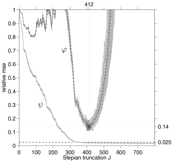
Figure 6: Relative regional mean squared model errors $\varphi(J)$, from Eq. (177), and relative mean squared data misfit $\psi(J)$, from Eq. (178), for potential field estimation from radial-derivative data as described in Eq. (114). The true signal is the one shown in Fig. 5. Each of the 64 realizations of noise leads to a gray $\varphi(J)$-curve and a gray $\psi(J)$. The optimal truncation points are indicated by gray circles, the average optimal truncation point by a black circle and the average $\varphi(J)$ behavior is the black dashed line. The dashed horizontal line is the relative energy of the noise.

In Fig. 6, each of the 64 gray lines labeled $\varphi$ is a curve of $\varphi(J)$, the regional relative mean squared model error calculated as in Eq. (177). The same true signal values $\mathsf{V}^{\prime}_{r}$ were used, but every experiment used data $\mathsf{d}_{r}$, as given by Eq. (106), that were contaminated by a different realization of the noise field $\mathsf{n}_{r}$, as described at the beginning of this section. Every curve starts at $\varphi(0)=1$, as without any basis functions, only the zero model is obtained. The relative mse decreases dramatically after about $J=250$ and the estimation improves as more Slepian functions are involved. As we have explained earlier for the theoretical behavior in Eq. (142), the squared bias term $\beta^{2}$ diminishes in value with increasing $J$. Less truncation (larger $J$) reduces the estimation bias, but this decrease is in competition with the variance $\nu$ term, which increases with $J$. The influence of data noise is felt more and more with the inclusion of additional basis functions.

The turning points of minimum relative mean squared estimation error for each of the experiments are indicated by a gray circle. At the corresponding value $J$, the optimal Slepian truncation level for each specific data set is reached. The average of all of the $\varphi(J)$ curves shown is represented by a black dashed line. All individual turning points are clustered around the average ideal truncation point, which is the $J=412$ indicated by the black circle. The relative regional mean squared model errors $\varphi$ do not improve immediately after $J=1$, unlike the data errors $\psi$. There is a local minimum, followed by a rise, and a precipitous decline after $J=250$ or thereabouts. We explain this behavior theoretically by our minimizing the misfit of the upward-transformed potential field at the altitude of the data (see Eq. 121) instead of the misfit on the surface, which is measured by $\varphi$. To obtain the potential field on the surface we need to downward-transform the radial-field estimate at altitude, obtained by truncation, as shown by Eq. (123). The downward transformation operator $\mathbf{A}$ defined in Eq. (32) is poorly conditioned for high maximum degrees $L$ and large relative satellite altitudes ${r_{s}}/{r_{e}}$. The interaction between all of the terms altogether displays a complex behavior that, however, has a clear global minimum which leads to a working algorithm and an objective decision as to the optimal Slepian function truncation level.

Because the noise level is relatively small compared to the signal strength, and because we use the same 2217 data locations, the $\psi$-lines with the data fits are close together. The relative mean squared data misfit curves $\psi(J)$ in Fig. 6 are decreasing fast until their values reach the relative energy of the noise, 2.5%, indicated by the dashed horizontal black line. At this point the relative mean squared data misfit decreases much slower, or almost not at all. We recall that the noise is generated in the spatial domain, and is therefore not bandlimited. Hence, the noise has appreciable energy at the degrees larger than 72 which cannot be fit by the $L=72$ bandlimited Slepian functions.

7.2 Estimating the Potential Field at the Surface from Gradient-Vector Data at Satellite Altitude

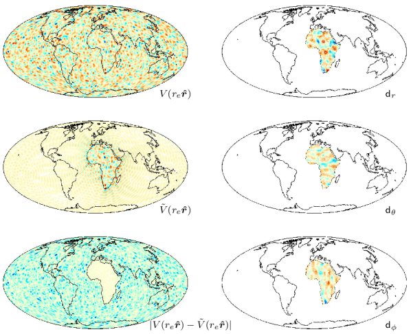
Figure 7: Example of a potential field estimation on Earth’s surface from noisy gradient data at altitude ${r_{s}}={r_{e}}+500$ km for Slepian functions with maximum degree $L=72$ and target region Africa. The upper left panel shows the true potential field $V({r_{e}}\boldsymbol{\hat{r}})$ on Earth’s surface. The three right panels show the noisy data $\mathsf{d}$ at satellite altitude given by 2217 data values. The top right panel depicts the radial component $\mathsf{d}_{r}$, the middle right panel the tangential colatitudinal component $\mathsf{d}_{\theta}$, and the lower right panel the tangential longitudinal component $\mathsf{d}_{\phi}$. The middle left panel shows the estimated potential field $\tilde{V}({r_{e}}\boldsymbol{\hat{r}})$ calculated from the data with Slepian truncation $J=472$. The lower left panel shows the absolute difference $|V({r_{e}}\boldsymbol{\hat{r}})-\tilde{V}({r_{e}}\boldsymbol{\hat{r}})\rvert$ between the true and the estimated potential fields.

Figure 8: Relative regional mean squared model error $\varphi(J)$, from Eq. (177), and relative mean squared data misfit $\psi(J)$, from Eq. (178), for potential-field estimation from vectorial data described in Eq. (151). The true signal is the same as for Fig. 7. Each of the 64 realizations of noise leads to a gray $\varphi(J)$-line and a gray $\psi(J)$. The optimal truncation points are indicated by the gray circles, the average optimal truncation point by the black circle and the average $\varphi(J)$ line by the black dashed line. The dashed horizontal line is the relative energy of the noise.

Fig. 7 shows the results from an experiment with noisy vectorial data. Our plot color conventions are unchanged from those in Section 7.1, except now the three panels on the right are scaled to the maximum absolute vectorial data value at satellite altitude. The true potential field $V({r_{e}}\boldsymbol{\hat{r}})$ is found in the upper left panel of Fig. 7, and the noisy data at altitude $\mathsf{d}$ are shown on the right. The top right panel shows the radial component $\mathsf{d}_{r}$, the middle right panel the tangential colatitudinal component $\mathsf{d}_{\theta}$, and the lower right panel the tangential longitudinal component $\mathsf{d}_{\phi}$.

We use Eq. (151) to calculate an estimate $\tilde{V}({r_{e}}\boldsymbol{\hat{r}})$ for the potential field on Earth’s surface, choosing the Slepian truncation $J=472$ based on the numerical experiments shown in Fig. 8. The estimated scalar potential field on Earth’s surface $\tilde{V}({r_{e}}\boldsymbol{\hat{r}})$ is shown in the middle left panel of Fig. 7. The lower left panel of Fig. 8 shows the absolute difference $\lvert V({r_{e}}\boldsymbol{\hat{r}})-\tilde{V}({r_{e}}\boldsymbol{\hat{r}})\rvert$ between the true and the estimated signal. The estimated field $\tilde{V}({r_{e}}\boldsymbol{\hat{r}})$ approximates the true signal $V({r_{e}}\boldsymbol{\hat{r}})$ well within Africa and is close to zero outside of that target region. The relative regional mean squared model error calculated using Eq. (177) is $0.058$.

In Fig. 8 we plot the relative regional mean squared model errors $\varphi(J)$ defined in Eq. (177) as a function of the truncation level $J$, for each of the 64 experiments. Each data set $\mathsf{d}$ is generated from the same true vector field $\mathsf{V}^{\prime}$ using Eq. (143), but differs by the realization of the noise $\mathsf{n}$, as discussed at the top of this section. Each experiment starts at $\varphi(0)=1$ and descends from about $J=250$ into a deep valley with increasing number of Slepian functions. The theoretical relation in Eq. (174) explains how the decreasing bias and increasing variance trade off as a function of the increasing number $J$ of Slepian functions. The turning points are indicated by gray circles; they all cluster around the same truncation value. The average relative regional mean squared model error is shown by a dashed black line, and the average optimal Slepian truncation level $J=472$ by a black circle. As in the scalar case the curves $\varphi(J)$ go through a local minimum before reaching the global optimum truncation level. Indeed, since we minimized Eq. (158) at altitude, in order to obtain the estimate $\tilde{V}({r_{e}}\boldsymbol{\hat{r}})$ at the Earth’s surface we need to apply the downward transformation operator $\mathbf{B}$ defined in Eq. (48). At high maximum degrees $L$ and high relative satellite altitudes ${r_{s}}/{r_{e}}$ this operator is poorly conditioned. The interaction between the various competing effects produces a complex but reproducible error behavior.

The 64 curves for the relative mean squared data misfit in Fig. 8 are close together because the signal-to-noise level is high, and because we reuse the same 2217 data locations. As for the scalar case, the relative mean squared data misfit $\psi(J)$ decreases fast until it reaches the relative energy of the noise, $2.5\%$, indicated by the dashed horizontal black line.

8 Conclusions

We presented two methods to estimate a potential field from gradient data at satellite altitude that are concentrated over a certain region. At the heart of both methods lies the use of spatiospectrally concentrated spherical basis functions. The first method only considered the radial component of the data and used scalar Slepian functions. The second method considered all three vectorial components of the data and used gradient-vector Slepian functions, a special case of vector Slepian functions. From the theoretical analysis of both methods, and through extensive experimentation, we show how the mean squared reconstruction error depends on the number of Slepian or gradient-vector Slepian functions used for the estimation. The more Slepian functions involved, the smaller the bias, but the larger the variance in the presence of noise.

Table of Symbols

symbol	description	Eq.
$L$	spherical-harmonic bandwidth
$R$	target region of data availability and for Slepian function concentration
$V({r_{e}}\boldsymbol{\hat{r}})$	three-dimensional potential-field function at Earth’s surface ${r_{e}}$	(9)
$V({r_{s}}\boldsymbol{\hat{r}})$	three-dimensional potential-field function at satellite altitude ${r_{s}}$	(18)
$u_{lm}^{r_{e}}$	expansion coefficients of $V({r_{e}}\boldsymbol{\hat{r}})$ in the basis of spherical harmonics $Y_{lm}$	(19)
$u_{lm}^{r_{s}}$	expansion coefficients of $V({r_{s}}\boldsymbol{\hat{r}})$ in the basis of spherical harmonics $Y_{lm}$	(27)
$\partial_{r}V({r_{s}}\boldsymbol{\hat{r}})$	radial derivative of the potential field at satellite altitude ${r_{s}}$	(21)
$\mbox{\boldmath$\nabla$}V({r_{s}}\boldsymbol{\hat{r}})$	three-dimensional gradient of the potential field at satellite altitude ${r_{s}}$	(20)
$v^{r_{s}}_{lm}$	expansion coefficients of $\mbox{\boldmath$\nabla$}V({r_{s}}\boldsymbol{\hat{r}})$ in the basis of gradient-vector harmonics $\boldsymbol{E}_{lm}$	(24)
$\mathrm{u}^{r_{a}}$	vector containing the coefficients $u_{lm}^{r_{a}}$ at radius ${r_{a}}$	(19)
$\mathrm{v}^{r_{a}}$	vector containing the coefficients $v^{r_{a}}_{lm}$ at radius ${r_{a}}$	(24)
$\mathbf{A}$	$(L+1)^{2}\times(L+1)^{2}$ diagonal matrix transforming the $\mathrm{u}^{r_{e}}$ to the $Y_{lm}$ coefficients of $\partial_{r}V({r_{s}}\boldsymbol{\hat{r}})$	(32)
$\mathbf{B}$	$(L+1)^{2}\times(L+1)^{2}$ diagonal matrix transforming the $\mathrm{u}^{r_{e}}$ to the $\boldsymbol{E}_{lm}$ coefficients of $\mbox{\boldmath$\nabla$}V({r_{s}}\boldsymbol{\hat{r}})$	(48)
$Y_{lm}$	scalar spherical-harmonic function for degree $l$ and order $m$	(1)
$\mathcal{Y}$	vector of all $(L+1)^{2}$ scalar spherical-harmonic functions to degree $L$	(51)
$\boldsymbol{\mathsf{Y}}$	$(L+1)^{2}\times k$ matrix of $Y_{lm}$ with bandwidth $L$ evaluated at $\boldsymbol{\hat{r}}_{1},\ldots,\boldsymbol{\hat{r}}_{k}$	(28)
$\hat{\mathcal{Y}}$	vector of all scalar spherical-harmonic functions to degree $\infty$	(52)
$\hat{\mathcal{Y}}_{>L}$	vector of all scalar spherical-harmonic functions for degrees $L<l\leq\infty$	(52)
$\boldsymbol{E}_{lm}$	gradient-vector spherical-harmonic function for degree $l$ and order $m$	(16)
$\boldsymbol{\mathcal{E}}$	$(L+1)^{2}$ vector of all $\boldsymbol{E}_{lm}$ up to degree $L$	(58)
$\boldsymbol{\mathsf{E}}$	$(L+1)^{2}\times 3k$ matrix of all of the $\boldsymbol{E}_{lm}$ evaluated at $\boldsymbol{\hat{r}}_{1},\ldots,\boldsymbol{\hat{r}}_{k}$	(42)
$\hat{\boldsymbol{\mathcal{E}}}$	vector of all gradient-vector spherical harmonics up to degree $\infty$	(59)
$\hat{\boldsymbol{\mathcal{E}}}_{>L}$	vector of all gradient-vector spherical harmonics for degrees $L<l\leq\infty$	(59)
$G_{\alpha}$	$\alpha$th best spatially concentrated (within $R$) bandlimited (to $L$) scalar spherical Slepian function	(73)
$\hat{G}_{\alpha}$	$\alpha$th best spectrally concentrated (within $L$) spacelimited (to $R$) scalar spherical Slepian function	(81)
$\mathrm{g}_{\alpha}$	$(L+1)^{2}\times 1$ vector containing the $Y_{lm}$ coefficients of one of the $G_{\alpha}$	(73)
$\hat{\mathrm{g}}_{\alpha}$	infinite-dimensional vector containing the $Y_{lm}$ coefficients of one of the $\hat{G}_{\alpha}$	(82)
$\mathcal{G}$	$(L+1)^{2}\times 1$ vector containing all of the $G_{\alpha}$ ordered with decreasing concentration ratio $\lambda_{\alpha}$	(75)
$\mathcal{G}_{J}$	$J\times 1$ vector of functions containing the $G_{1},\ldots,G_{J}$	(78)
$\mathcal{G}_{\downarrow J}$	$J\times 1$ vector of localized downward-transformed scalar Slepian functions	(115)
$\mathcal{G}_{\uparrow J}$	$J\times 1$ vector of localized upward-transformed scalar Slepian functions	(116)
$\mathcal{G}_{\downarrow>J}$	$\left[(L+1)^{2}-J+1\right]\times 1$ vector complementing $\mathcal{G}_{\downarrow J}$	(115)
$\mathcal{G}_{\uparrow>J}$	$\left[(L+1)^{2}-J+1\right]\times 1$ vector complementing $\mathcal{G}_{\uparrow J}$	(116)
$\boldsymbol{\mathsf{G}}$	$(L+1)^{2}\times k$ matrix of all of the $G_{\alpha}$ evaluated at $\boldsymbol{\hat{r}}_{1},\ldots,\boldsymbol{\hat{r}}_{k}$	(107)
$\boldsymbol{\mathsf{G}}_{J}$	$J\times k$ matrix of $G_{1},\ldots,G_{J}$ evaluated at $\boldsymbol{\hat{r}}_{1},\ldots,\boldsymbol{\hat{r}}_{k}$	(110)
$\mathbf{G}$	$(L+1)^{2}\times(L+1)^{2}$ matrix containing the $Y_{lm}$ coefficients for all of the $G_{\alpha}$	(71)
$\mathbf{G}_{J}$	$(L+1)^{2}\times J$ matrix containing the $Y_{lm}$ coefficients for the $G_{1},\ldots,G_{J}$	(77)
$\lambda_{\alpha}$	energy concentration ratio of one of the $G_{\alpha}$	(68)
$\mathbf{\Lambda}$	$(L+1)^{2}\times(L+1)^{2}$ diagonal matrix containing all of the $\lambda_{\alpha}$	(72)
$\mathbf{\Lambda}_{J}$	$J\times J$ diagonal matrix containing the $J$ largest $\lambda_{1},\ldots,\lambda_{J}$	(79)
$\mathbf{D}$	$(L+1)^{2}\times(L+1)^{2}$ localization matrix diagonalized by $\mathbf{G}$	(70)
$\hat{\mathbf{D}}_{L}$	$\infty\times(L+1)^{2}$ matrix extending $\mathbf{D}$ down to contain the inner products of $\hat{\mathcal{Y}}$ and $\mathcal{Y}$	(84)
$\hat{\mathbf{D}}_{>L,L}$	$\infty\times(L+1)^{2}$ matrix containing the lowermost portion of $\hat{\mathbf{D}}_{L}$ for degrees $l>L$	(85)
$\hat{G}_{>L,\alpha}$	scalar function made from the degrees $l>L$ of $\hat{G}_{\alpha}$	(88)
$\hat{\mathrm{g}}_{>L,\alpha}$	infinite-dimensional vector containing the $l>L$ entries of $\hat{\mathrm{g}}_{\alpha}$	(86)
$\hat{\mathcal{G}}_{>L,J}$	$J\times 1$ vector of functions containing the first $J$ of the $\hat{G}_{>L,\alpha}$	(89)
$\hat{\mathbf{G}}_{>L,J}$	$\infty\times J$ matrix containing the $Y_{lm}$ coefficients for $l>L$ of the $\hat{G}_{\alpha}$	(87)
$\boldsymbol{H}_{\alpha}$	$\alpha$th best-concentrated gradient-vector Slepian function for bandwidth $L$ and region $R$	(96)
$\mathrm{h}_{\alpha}$	$(L+1)^{2}\times 1$ vector containing the $\boldsymbol{E}_{lm}$ coefficients of one of the $\boldsymbol{H}_{\alpha}$	(92)
$\boldsymbol{\mathcal{H}}$	$(L+1)^{2}\times 1$ vector containing all of the $\boldsymbol{H}_{\alpha}$ ordered with decreasing concentration ratio $\sigma_{\alpha}$	(98)
$\boldsymbol{\mathcal{H}}_{J}$	$J\times 1$ vector of functions containing the $\boldsymbol{H}_{1},\ldots,\boldsymbol{H}_{J}$	(101)
$\mathcal{H}_{\downarrow J}$	$J\times 1$ vector of scalar-valued downward-transformed gradient-vector Slepian functions	(152)
$\mathcal{H}_{\uparrow J}$	$J\times 1$ vector of scalar-valued upward-transformed gradient-vector Slepian functions	(153)
$\mathcal{H}_{\downarrow>J}$	$\left[(L+1)^{2}-J+1\right]\times 1$ vector complementing $\mathcal{H}_{\downarrow J}$	(152)
$\mathcal{H}_{\uparrow>J}$	$\left[(L+1)^{2}-J+1\right]\times 1$ vector complementing $\mathcal{H}_{\uparrow J}$	(153)
$\boldsymbol{\mathsf{H}}$	$(L+1)^{2}\times 3k$ matrix of all of the $\boldsymbol{H}_{\alpha}$ evaluated at $\boldsymbol{\hat{r}}_{1},\ldots,\boldsymbol{\hat{r}}_{k}$	(144)
$\boldsymbol{\mathsf{H}}_{J}$	$J\times 3k$ matrix of $\boldsymbol{H}_{1},\ldots,\boldsymbol{H}_{J}$ evaluated at $\boldsymbol{\hat{r}}_{1},\ldots,\boldsymbol{\hat{r}}_{k}$	(147)
$\mathbf{H}$	$(L+1)^{2}\times(L+1)^{2}$ matrix containing the $\boldsymbol{E}_{lm}$ coefficients for all of the $\boldsymbol{H}_{\alpha}$	(94)
$\mathbf{H}_{J}$	$(L+1)^{2}\times J$ matrix containing the $\boldsymbol{E}_{lm}$ coefficients for the $\boldsymbol{H}_{1},\ldots,\boldsymbol{H}_{J}$	(100)
$\sigma_{\alpha}$	energy concentration ratio of $\boldsymbol{H}_{\alpha}$ over $R$	(91)
$\mathbf{\Sigma}$	$(L+1)^{2}\times(L+1)^{2}$ diagonal matrix containing all of the $\sigma_{\alpha}$	(95)
$\mathbf{\Sigma}_{J}$	$J\times J$ diagonal matrix containing the $J$ largest $\sigma_{1},\ldots,\sigma_{J}$	(102)
$\mathbf{K}$	$(L+1)^{2}\times(L+1)^{2}$ localization matrix diagonalized by $\mathbf{H}$	(93)
$\hat{\mathbf{K}}_{>L,L}$	$\infty\times(L+1)^{2}$ matrix containing the inner products of $\hat{\boldsymbol{\mathcal{E}}}_{>L}$ with $\boldsymbol{\mathcal{E}}$	(104)
$\hat{\boldsymbol{\mathcal{H}}}_{\hat{\boldsymbol{\mathcal{E}}},>L,J}$	$J\times 1$ vector of functions containing the $\hat{\boldsymbol{\mathcal{E}}}_{>L}$ components of the spacelimited $\boldsymbol{\mathcal{H}}$	(105)
$d(\boldsymbol{\hat{r}})$	scalar data function at satellite altitude ${r_{s}}$	(119)
$\boldsymbol{d}(\boldsymbol{\hat{r}})$	gradient data function at satellite altitude ${r_{s}}$	(156)
$\mathsf{d}_{r}$	$k\times 1$ vector of measured radial data values at satellite altitude ${r_{s}}$	(106)
$\mathsf{d}$	$3k\times 1$ vector of measured gradient data values at satellite altitude ${r_{s}}$	(143)
$n(\boldsymbol{\hat{r}})$	scalar noise function at satellite altitude ${r_{s}}$	(119)
$\boldsymbol{n}(\boldsymbol{\hat{r}})$	vectorial noise function at satellite altitude ${r_{s}}$	(156)
$\mathsf{n}_{r}$	$k\times 1$ vector of radial-derivative noise at satellite altitude ${r_{s}}$	(106)
$\mathsf{n}$	$3k\times 1$ vector of vectorial noise at satellite altitude ${r_{s}}$	(143)
$\mathsf{V}$	$k\times 1$ vector containing the potential-field signal points $V({r_{s}}\boldsymbol{\hat{r}}),\ldots,V({r_{s}}\boldsymbol{\hat{r}})$	(26)
$\mathsf{V}^{\prime}_{r}$	$k\times 1$ vector containing the radial-derivative signal points $\partial_{r}V({r_{s}}\boldsymbol{\hat{r}}),\ldots,\partial_{r}V({r_{s}}\boldsymbol{\hat{r}})$	(33)
$\mathsf{V}^{\prime}$	$3k\times 1$ vector containing the full gradient signal points $\mathsf{V}^{\prime}_{r},\mathsf{V}^{\prime}_{\theta}$, and $\mathsf{V}^{\prime}_{\phi}$ at satellite altitude	(38)
$\tilde{V}({r_{e}}\boldsymbol{\hat{r}})$	potential field at the Earth’s surface estimated from the radial-derivative data at altitude	(114)
	potential field at the Earth’s surface estimated from the full gradient data at altitude	(151)
$\tilde{\mathrm{s}}^{r_{s}}_{J}$	$J\times 1$ vector of $G_{\alpha}$ coefficients of $V({r_{s}}\boldsymbol{\hat{r}})$ estimated from the scalar data $\mathsf{d}_{r}$	(112)
${\tilde{\mathrm{t}}}^{r_{s}}_{J}$	$J\times 1$ vector of $\boldsymbol{H}_{\alpha}$ coefficients of $\mbox{\boldmath$\nabla$}V({r_{s}}\boldsymbol{\hat{r}})$ estimated from the vector data $\mathsf{d}$	(149)
$\mathrm{\tilde{u}}^{r_{e}}$	$(L+1)^{2}\times 1$ vector of $Y_{lm}$ coefficients of the estimate $\tilde{V}({r_{e}}\boldsymbol{\hat{r}})$ derived from the $\tilde{\mathrm{s}}^{r_{s}}$	(113)
	$(L+1)^{2}\times 1$ vector of $Y_{lm}$ coefficients of the estimate $\tilde{V}({r_{e}}\boldsymbol{\hat{r}})$ derived from the ${\tilde{\mathrm{t}}}^{r_{s}}_{J}$	(150)
$\nu$	variance of the estimate $\tilde{V}({r_{e}}\boldsymbol{\hat{r}})$ from the scalar data $d(\boldsymbol{\hat{r}})$ in truncated Slepian estimation	(140)
	variance of the estimate $\tilde{V}({r_{e}}\boldsymbol{\hat{r}})$ from the vector data $\boldsymbol{d}(\boldsymbol{\hat{r}})$ in truncated Slepian estimation	(172)
$\beta$	bias of the estimate $\tilde{V}({r_{e}}\boldsymbol{\hat{r}})$ from the scalar data $d(\boldsymbol{\hat{r}})$ in truncated Slepian estimation	(137)
	bias of the estimate $\tilde{V}({r_{e}}\boldsymbol{\hat{r}})$ from the vector data $\boldsymbol{d}(\boldsymbol{\hat{r}})$ in truncated Slepian estimation	(170)
$\langle\epsilon^{2}\rangle$	mean squared error of the estimate $\tilde{V}({r_{e}}\boldsymbol{\hat{r}})$ from the scalar data $d(\boldsymbol{\hat{r}})$	(142)
	mean squared error of the estimate $\tilde{V}({r_{e}}\boldsymbol{\hat{r}})$ from the vector data $\boldsymbol{d}(\boldsymbol{\hat{r}})$	(174)
$\varphi(j)$	relative regional mean squared model error between $\tilde{V}({r_{e}}\boldsymbol{\hat{r}})$ and $V({r_{e}}\boldsymbol{\hat{r}})$	(177)
$\psi(J)$	relative mean squared data misfit between $\mathsf{d}_{r}$ and $\boldsymbol{\mathsf{Y}}^{\sf T}\mathbf{A}\mathrm{\tilde{u}}^{r_{e}}$ for the scalar case	(178)
	relative mean squared data misfit between $\mathsf{d}$ and $\boldsymbol{\mathsf{E}}^{\sf T}\mathbf{B}\mathrm{u}^{r_{e}}$ or for the vector case	(179)

References

• Albertella et al. (1999) Albertella, A., Sansò, F., & Sneeuw, N., 1999. Band-limited functions on a bounded spherical domain: the Slepian problem on the sphere, J. Geodesy, 73, 436–447.
• Albertella et al. (2008) Albertella, A., Savcenko, R., Bosch, W., & Rummel, R., 2008. Dynamic Ocean Topography – The Geodetic Approach, Tech. Rep. 27, Institut für Astronomische und Physikalische Geodäsie, Forschungseinrichtung Satellitengeodäsie, München.
• Arkani-Hamed (2001) Arkani-Hamed, J., 2001. A 50-degree spherical harmonic model of the magnetic field of Mars, J. Geophys. Res., 106(E10), 23197–23208, doi: 10.1029/2000JE001365.
• Arkani-Hamed (2002) Arkani-Hamed, J., 2002. An improved 50-degree spherical harmonic model of the magnetic field of Mars derived from both high-altitude and low-altitude data, J. Geophys. Res., 107(E10), 5083, doi: 10.1029/2001JE001835.
• Arkani-Hamed (2004) Arkani-Hamed, J., 2004. A coherent model of the crustal magnetic field of Mars, J. Geophys. Res., 109, E09005, doi: 10.1029/2004JE002265.
• Arkani-Hamed & Strangway (1986) Arkani-Hamed, J. & Strangway, D. W., 1986. Band-limited global scalar magnetic anomaly map of the Earth derived from Magsat data, J. Geophys. Res., 91(B8), 8193–8203.
• Backus et al. (1996) Backus, G. E., Parker, R. L., & Constable, C. G., 1996. Foundations of geomagnetism, Cambridge Univ. Press, Cambridge, UK.
• Beggan et al. (2013) Beggan, C. D., Saarimäki, J., Whaler, K. A., & Simons, F. J., 2013. Spectral and spatial decomposition of lithospheric magnetic field models using spherical Slepian functions, Geophys. J. Int., 193(1), 136–148, 10.1093/gji/ggs122.
• Blakely (1995) Blakely, R. J., 1995. Potential Theory in Gravity and Magnetic Applications, Cambridge Univ. Press, New York.
• Bölling & Grafarend (2005) Bölling, K. & Grafarend, E. W., 2005. Ellipsoidal spectral properties of the Earth’s gravitational potential and its first and second derivatives, J. Geodesy, 79(6–7), 300–330, doi: 10.1007/s00190–005–0465–y.
• Chambodut et al. (2005) Chambodut, A., Panet, I., Mandea, M., Diament, M., Holschneider, M., & Jamet, O., 2005. Wavelet frames: an alternative to spherical harmonic representation of potential fields, Geophys. J. Int., 163(3), 875–899.
• Cox & Hinkley (1974) Cox, D. R. & Hinkley, D. V., 1974. Theoretical Statistics, Chapman and Hall, London, UK.
• Dahlen & Tromp (1998) Dahlen, F. A. & Tromp, J., 1998. Theoretical Global Seismology, Princeton Univ. Press, Princeton, N. J.
• Davison (2003) Davison, A. C., 2003. Statistical Models, Cambridge Univ. Press, Cambridge, UK.
• de Santis (1991) de Santis, A., 1991. Translated originspherical cap harmonic analysis, Geophys. J. Int., 106, 253–263.
• Eshagh (2009) Eshagh, M., 2009. Comparison of two approaches for considering laterally varying density in topographic effect on satellite gravity gradiometric data, Acta Geophysica, pp. 10.2478/s11600–009–0057–y.
• Fengler et al. (2007) Fengler, M. J., Freeden, W., Kohlhaas, A., Michel, V., & Peters, T., 2007. Wavelet modeling of regional and temporal variations of the earth’s gravitational potential observed by GRACE, J. Geodesy, 81(1), 5–15, doi: 10.1007/s00190–006–0040–1.
• Freeden & Michel (2004) Freeden, W. & Michel, V., 2004. Multiscale Potential Theory, Birkhäuser, Boston, Mass.
• Freeden & Schreiner (2009) Freeden, W. & Schreiner, M., 2009. Spherical Functions of Mathematical Geosciences: A Scalar, Vectorial, and Tensorial Setup, Springer, Berlin.
• Gubbins et al. (2011) Gubbins, D., Ivers, D., Masterton, S. M., & Winch, D. E., 2011. Analysis of lithospheric magnetization in vector spherical harmonics, Geophys. J. Int., 187, 99–117, doi: 10.1111/j.1365–246X.2011.05153.x.
• Haines (1985) Haines, G. V., 1985. Spherical cap harmonic analysis, J. Geophys. Res., 90(B3), 2583–2591.
• Harig & Simons (2012) Harig, C. & Simons, F. J., 2012. Mapping Greenland’s mass loss in space and time, Proc. Natl. Acad. Sc., 109(49), 19934–19937, doi: 10.1073/pnas.1206785109.
• Hwang (1993) Hwang, C., 1993. Spectral analysis using orthonormal functions with a case study on sea surface topography, Geophys. J. Int., 115, 1148–1160.
• Hwang & Chen (1997) Hwang, C. & Chen, S.-K., 1997. Fully normalized spherical cap harmonics: Application to the analysis of sea-level data from TOPEX/POSEIDON and ERS-1, Geophys. J. Int., 129, 450–460.
• Jahn & Bokor (2012) Jahn, K. & Bokor, N., 2012. Vector slepian basis functions with optimal energy concentration in high numerical aperture focusing, Optics Comm., 285, 2028–2038, doi: 10.1016/j.optcom.2011.11.107.
• Kaula (1967) Kaula, W. M., 1967. Theory of statistical analysis of data distributed over a sphere, Rev. Geophys., 5(1), 83–107.
• Kennedy & Sadeghi (2013) Kennedy, R. A. & Sadeghi, P., 2013. Hilbert Space Methods in Signal Processing, Cambridge Univ. Press, Cambridge, UK.
• Korte & Holme (2003) Korte, M. & Holme, R., 2003. Regularization of spherical cap harmonics, Geophys. J. Int., 153, 253–262, doi: 10.1046/j.1365–246X.2003.01898.x.
• Langel & Hinze (1998) Langel, R. A. & Hinze, W. J., 1998. The Magnetic Field of the Earth’s Lithosphere: The Satellite Perspective, Cambridge Univ. Press, Cambridge, UK.
• Lewis & Simons (2012) Lewis, K. W. & Simons, F. J., 2012. Local spectral variability and the origin of the Martian crustal magnetic field, Geophys. Res. Lett., 39, L18201, doi: 10.1029/2012GL052708.
• Lowes & Winch (2012) Lowes, F. J. & Winch, D. E., 2012. Orthogonality of harmonic potentials and fields in spheroidal and ellipsoidal coordinates: application to geomagnetism and geodesy, Geophys. J. Int., 191(2), 491–507, doi: 10.1111/j.1365–246X.2012.05590.x.
• Lowes et al. (1995) Lowes, F. J., de Santis, A., & Duka, B., 1995. A discussion of the uniqueness of a Laplacian potential when given only partial field information on a sphere, Geophys. J. Int., 121(2), 579–584.
• Mallat (2008) Mallat, S., 2008. A Wavelet Tour of Signal Processing, The Sparse Way, Academic Press, San Diego, Calif., 3rd edn.
• Maus (2010) Maus, S., 2010. An ellipsoidal harmonic representation of Earth’s lithospheric magnetic field to degree and order 720, Geochem. Geophys. Geosys., 11(6), Q06015, doi: 10.1029/2010GC003026.
• Maus et al. (2006a) Maus, S., Lühr, H., & Purucker, M., 2006a. Simulation of the high-degree lithospheric field recovery for the Swarm constellation of satellites, Earth Planets Space, 58, 397–407.
• Maus et al. (2006b) Maus, S., Rother, M., Hemant, K., Stolle, C., Lühr, H., Kuvshinov, A., & Olsen, N., 2006b. Earth’s lithospheric magnetic field determined to spherical harmonic degree 90 from CHAMP satellite measurements, Geophys. J. Int., 164, 319–330, doi: 10.1111/j.1365–246X.2005.02833.x.
• Maus et al. (2006c) Maus, S., Rother, M., Stolle, C., Mai, W., Choi, S., Lühr, H., Cooke, D., & Roth, C., 2006c. Third generation of the Potsdam Magnetic Model of the Earth (POMME), Geochem. Geophys. Geosys., 7, Q07008, doi: 10.1029/2006GC001269.
• Mayer & Maier (2006) Mayer, C. & Maier, T., 2006. Separating inner and outer Earth’s magnetic field from CHAMP satellite measurements by means of vector scaling functions and wavelets, Geophys. J. Int., 167, 1188–1203, doi: 10.1111/j.1365–246X.2006.03199.x.
• Moritz (2010) Moritz, H., 2010. Classical physical geodesy, in Handbook of Geomathematics, chap. 6, pp. 130–158, doi: 10.1007/978–3–642–01546–5_6, eds Freeden, W., Nashed, M. Z., & Sonar, T., Springer, Heidelberg, Germany.
• Nutz (2002) Nutz, H., 2002. A Unified Setup of Gravitational Field Observables, Ph.D. thesis, Univ. Kaiserslautern, Germany.
• O’Brien & Parker (1994) O’Brien, M. S. & Parker, R. L., 1994. Regularized geomagnetic field modelling using monopoles, Geophys. J. Int., 118(3), 566–578, doi: 10.1111/j.1365–246X.1994.tb03985.x.
• Olsen et al. (2009) Olsen, N., Mandea, M., Sabaka, T. J., & Tøffner-Clausen, L., 2009. CHAOS-2—a geomagnetic field model derived from one decade of continuous satellite data, Geophys. J. Int., 179, 1477–1487, doi: 10.1111/j.1365–246X.2009.04386.x.
• Olsen et al. (2010) Olsen, N., Hulot, G., & Sabaka, T. J., 2010. Sources of the geomagnetic field and the modern data that enable their investigation, in Handbook of Geomathematics, chap. 5, pp. 105–124, doi: 10.1007/978–3–642–01546–5_5, eds Freeden, W., Nashed, M. Z., & Sonar, T., Springer, Heidelberg, Germany.
• Plattner & Simons (2013) Plattner, A. & Simons, F. J., 2013. Spatiospectral concentration of vector fields on a sphere, Appl. Comput. Harmon. Anal., p. doi:10.1016/j.acha.2012.12.001.
• Rowlands et al. (2005) Rowlands, D. D., Luthcke, S. B., Klosko, S. M., Lemoine, F. G. R., Chinn, D. S., McCarthy, J. J., Cox, C. M., & Anderson, O. B., 2005. Resolving mass flux at high spatial and temporal resolution using GRACE intersatellite measurements, Geophys. Res. Lett., 32, L04310, doi: 10.1029/2004GL021908.
• Rummel & van Gelderen (1995) Rummel, R. & van Gelderen, M., 1995. Meissl scheme — spectral characteristics of physical geodesy, Manuscr. Geod., 20(5), 379–385.
• Sabaka et al. (2010) Sabaka, T. J., Hulot, G., & Olsen, N., 2010. Mathematical properties relevant to geomagnetic field modeling, in Handbook of Geomathematics, chap. 17, pp. 503–538, doi: 10.1007/978–3–642–01546–5_17, eds Freeden, W., Nashed, M. Z., & Sonar, T., Springer, Heidelberg, Germany.
• Schachtschneider et al. (2010) Schachtschneider, R., Holschneider, M., & Mandea, M., 2010. Error distribution in regional inversion of potential field data, Geophys. J. Int., 181, 1428–1440, doi: 10.1111/j.1365–246X.2010.04598.x.
• Schachtschneider et al. (2012) Schachtschneider, R., Holschneider, M., & Mandea, M., 2012. Error distribution in regional modelling of the geomagnetic field, Geophys. J. Int., 191, 1015–1024, doi: 10.1111/j.1365–246X.2012.05675.x.
• Simons & Dahlen (2006) Simons, F. J. & Dahlen, F. A., 2006. Spherical Slepian functions and the polar gap in geodesy, Geophys. J. Int., 166, 1039–1061, doi: 10.1111/j.1365–246X.2006.03065.x.
• Simons et al. (2006) Simons, F. J., Dahlen, F. A., & Wieczorek, M. A., 2006. Spatiospectral concentration on a sphere, SIAM Rev., 48(3), 504–536, doi: 10.1137/S0036144504445765.
• Simons et al. (2009) Simons, F. J., Hawthorne, J. C., & Beggan, C. D., 2009. Efficient analysis and representation of geophysical processes using localized spherical basis functions, in Wavelets XIII, vol. 7446, pp. 74460G, doi: 10.1117/12.825730, SPIE.
• Slepian (1964) Slepian, D., 1964. Prolate spheroidal wave functions, Fourier analysis and uncertainty — IV: Extensions to many dimensions; generalized prolate spheroidal functions, Bell Syst. Tech. J., 43(6), 3009–3057.
• Slepian (1983) Slepian, D., 1983. Some comments on Fourier analysis, uncertainty and modeling, SIAM Rev., 25(3), 379–393.
• Slepian & Pollak (1961) Slepian, D. & Pollak, H. O., 1961. Prolate spheroidal wave functions, Fourier analysis and uncertainty — I, Bell Syst. Tech. J., 40(1), 43–63.
• Slobbe et al. (2012) Slobbe, D. C., Simons, F. J., & Klees, R., 2012. The spherical Slepian basis as a means to obtain spectral consistency between mean sea level and the geoid, J. Geodesy, 86(8), 609–628, doi: 10.1007/s00190–012–0543–x.
• Thébault et al. (2006) Thébault, E., Schott, J. J., & Mandea, M., 2006. Revised spherical cap harmonic analysis (R-SCHA): Validation and properties, J. Geophys. Res., 111(B1), B01102, doi: 10.1029/2005JB003836.
• Trampert & Snieder (1996) Trampert, J. & Snieder, R., 1996. Model estimations biased by truncated expansions: Possible artifacts in seismic tomography, Science, 271(5253), 1257–1260, doi: 10.1126/science.271.5253.1257.
• Whaler & Gubbins (1981) Whaler, K. A. & Gubbins, D., 1981. Spherical harmonic analysis of the geomagnetic field: an example of a linear inverse problem, Geophys. J. Int., 65(3), 645–693, doi: 10.1111/j.1365–246X.1981.tb04877.x.
• Wieczorek & Simons (2007) Wieczorek, M. A. & Simons, F. J., 2007. Minimum-variance spectral analysis on the sphere, J. Fourier Anal. Appl., 13(6), 665–692, doi: 10.1007/s00041–006–6904–1.
• Xu (1992a) Xu, P., 1992a. Determination of surface gravity anomalies using gradiometric observables, Geophys. J. Int., 110, 321–332.
• Xu (1992b) Xu, P., 1992b. The value of minimum norm estimation of geopotential fields, Geophys. J. Int., 111, 170–178.
• Xu (1998) Xu, P., 1998. Truncated SVD methods for discrete linear ill-posed problems, Geophys. J. Int., 135(2), 505–514, doi: 10.1046/j.1365–246X.1998.00652.x.